Singularities of Floquet Scattering and Tunneling

Abstract

We study quasi-bound states and scattering with short range potentials in three dimensions, subject to an axial periodic driving. We find that poles of the scattering S-matrix can cross the real energy axis as a function of the drive amplitude, making the S-matrix nonanalytic at a singular point. For the corresponding quasi-bound states that can tunnel out of (or get captured within) a potential well, this results in a discontinuous jump in both the angular momentum and energy of emitted (absorbed) waves. We also analyze elastic and inelastic scattering of slow particles in the time dependent potential. For a drive amplitude at the singular point, there is a total absorption of incoming low energy (s-wave) particles and their conversion to high energy outgoing (mostly p-) waves. We examine the relation of such Floquet singularities, lacking in an effective time independent approximation, with well known “spectral singularities” (or “exceptional points”). These results are based on an analytic approach for obtaining eigensolutions of time-dependent periodic Hamiltonians with mixed cylindrical and spherical symmetry, and apply broadly to particles interacting via power law forces and subject to periodic fields, e.g. co-trapped ions and atoms.

I Introduction and main results

The main object of this paper is a time-dependent Schrödinger equation in three dimensions, that can be brought to the form

$$i\dot{\phi}\left(\vec{r},t\right)=\left[-\frac{1}{2}\nabla^{2}+V_{{\rm in}}\left(\vec{r},t\right)+V_{{\rm out}}\left(\vec{r},t\right)\right]\phi\left(\vec{r},t\right),$$ (1)

where each potential term is dominant in a different spatial region, and both are $\pi$-periodic in time (in rescaled units in which the fundamental angular frequency is $2$, and $\hbar=m=1$). We present an approach for obtaining approximate quasi-periodic, Floquet eigenfunctions of Eq. (1), starting with explicitly known families of solutions for each separate Schrödinger equation with $V_{{\rm in}}$ or $V_{{\rm out}}$, one possibly being time-independent as a particular case. This method allows us to explore a regime of parameters inaccessible to perturbation methods.

In particular we study solutions to a problem that can be formulated in two equivalent ways; one is given by the equation

$$i\dot{\psi}\left(\vec{R},t\right)=\left[-\frac{1}{2}\nabla^{2}+V_{{\rm int}}\left(\left|\vec{R}-\vec{R}^{\pi}\left(t\right)\right|\right)\right]\psi\left(\vec{R},t\right),$$ (2)

where $V_{\rm int}$ is a spherically symmetric interaction potential and $\vec{R}^{\pi}(t)$ is a prescribed $\pi$-periodic trajectory of the center of force. To obtain a form compatible with Eq. (1), we apply the (unitary) change of coordinates

$$\vec{r}=\vec{R}-\vec{R}^{\pi}\left(t\right),\qquad\partial_{t}\to-\dot{\vec{R}}^{\pi}\left(t\right)\cdot\vec{\nabla}+\partial_{t},$$ (3)

and then a second unitary transformation

$$\psi=\exp\left\{i\dot{\vec{R}}^{\pi}\left(t\right)\cdot\vec{r}\right\}\phi,$$ (4)

reducing Eq. (2) to the sum of a time-independent central force and an additional $\pi$-periodic linear force,

$$i\dot{\phi}\left(\vec{r},t\right)=\left[-\frac{1}{2}\nabla^{2}+V_{{\rm int}}\left(r\right)-\ddot{\vec{F}}\left(t\right)\cdot\vec{r}+V_{F}(t)\right]\phi\left(\vec{r},t\right),$$ (5)

where $r\equiv\left|\vec{r}\right|$ and

$$\vec{F}\left(t\right)=-\vec{R}^{\pi}\left(t\right),\qquad V_{F}\left(t\right)=-\frac{1}{2}\dot{\vec{R}}^{\pi}\left(t\right)^{2}.$$ (6)

Here, the choice of what constitutes $V_{\rm in}$ and $V_{\rm out}$ depends on the approximation that is required in order to obtain the solution. The term $V_{F}(t)$ comes from the change of frame starting from Eq. (2), and if the starting point is Eq. (5), it will be absent. Both of these aspects will be further discussed in Sec. III, and here we keep the discussion general.

If we consider $-\ddot{\vec{F}}\left(t\right)$ to be a monochromatic electric field amplitude, and $V_{{\rm int}}\left(r\right)$ the Coulomb potential for an electron with coordinate $\vec{r}$, Eq. (5) with $V_{F}=0$ describes the well studied problem of an atom in an AC field (the AC-Stark effect), written in the length-gauge within the dipole approximation. Then the bound states of $V_{\rm int}$ are known to turn into resonances. These are quasi-bound states with a finite lifetime determined by the imaginary part of their complex energy. This happens generally under the effect of a periodic perturbation, for any Hamiltonian with a continuous spectrum of scattering states Yajima1982 ; Yajima1983 ; Yafaev1991 . The reason is that the periodic perturbation makes every bound state with energy $\left(-\left|\epsilon\right|\right)$ resonant with unbound states from the continuum, under absorption of at least $N$ quanta from the external drive (whose frequency is $2$), where

$$\left(-\left|\epsilon\right|\right)+2N>0,$$ (7)

and $2N$ gives the exponent of the power-law dependence of the resonance width on the perturbation amplitude.

Studies of nonperturbative violations of this picture go back to Keldysh theory Keldysh1965 and the extensive intense-laser literature 0034-4885-60-4-001 . The limit where the frequency and intensity of the oscillating field are much higher than the atomic potential can be studied by using an effective averaged potential, known as the Kramers-Hanneberger (KH) approximation. This approach has led to the prediction of the remarkable phenomenon of stabilization of the atom against ionization PhysRevLett.52.613 ; PhysRevA.37.4536 ; gavrila2002atomic , with renewed interest in recent years following experimental results eichmann2009acceleration ; eichmann2013observing ; 0953-4075-47-20-204014 and theoretical investigations PhysRevLett.110.253001 ; PhysRevA.90.023401 . Other recent works have also revisited the systematic expansion of an effective time-independent Hamiltonian in the high-frequency limit in a general setup PhysRevLett.91.110404 ; PhysRevA.68.013820 , and effects related to the potential’s initial phase PhysRevA.76.013421 . For intermediate laser intensities and frequencies, the problem is inherently difficult and most approaches are based on numerical integration in some form, e.g. using close-coupled equations PhysRevLett.59.872 ; PhysRevA.44.R5343 ; PhysRevA.36.5178 ; PhysRevA.43.1512 , or Floquet R-matrix theory, dividing space into two regions and connecting the numerically intergated solutions at the boundary burke1991r ; PhysRevA.86.043408 . There is renewed interest in the modeling and measuring of AC Stark shifts of trapped atoms markert2010ac , in calculating and directly probing the angular distribution of photoelectron spectra PhysRevA.78.043403 ; Morales11102011 , and in the momentum distribution of emitted electrons delone1991energy ; rudenko2004resonant ; rudenko2005coulomb ; liu2012low ; xia2015momentum ; ivanov2016transverse , where cusps in the transverse momentum distribution curves were attributed to the long range nature of the Coulomb interaction.

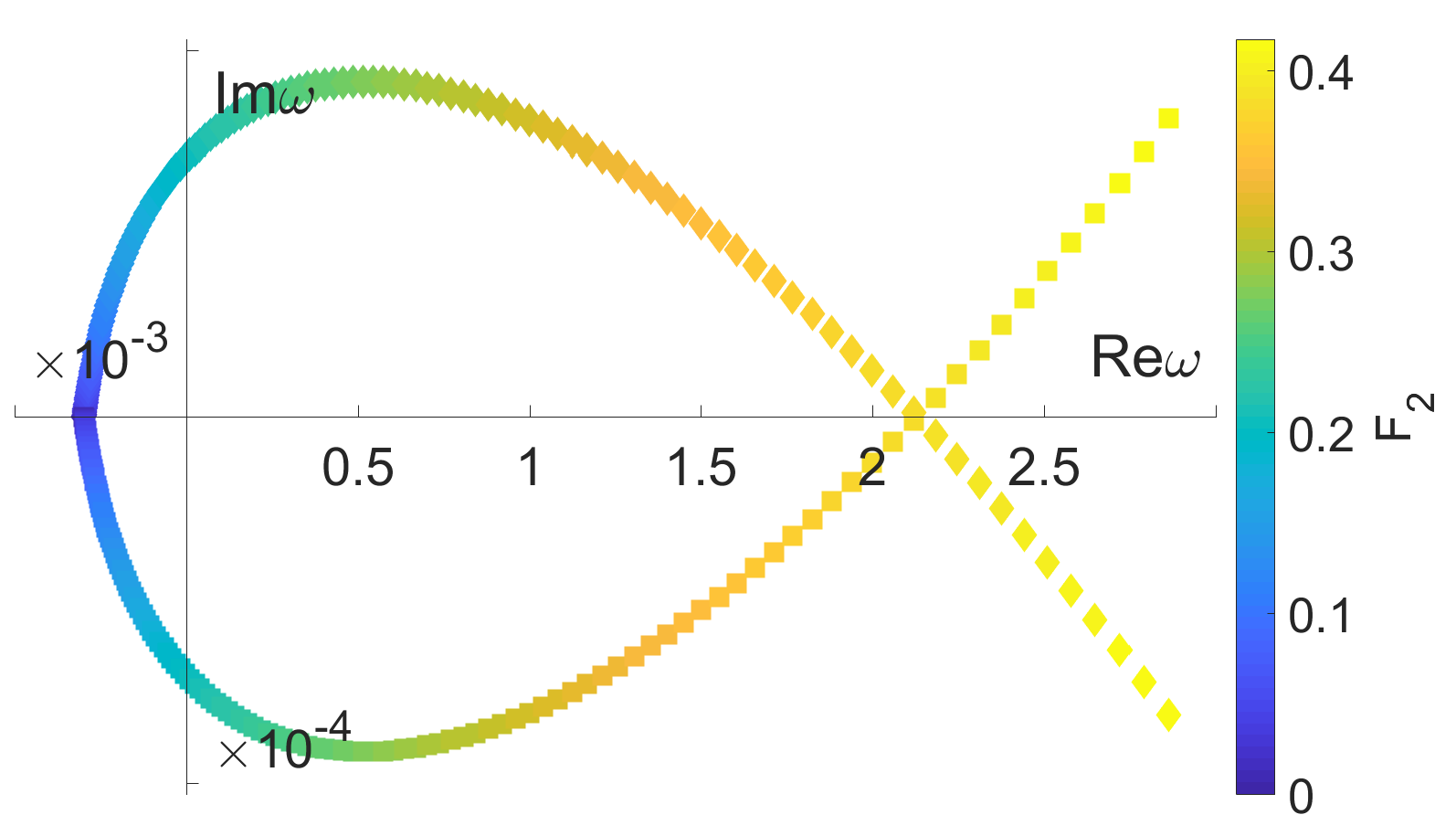
Figure 1: The complex quasi-energy $\omega$ (in nondimensional units) of two quasi-bound solutions to Eq. (2) with a spherically symmetric square-well potential and an axial periodic drive (see text for details), continued with small increments of the drive amplitude $F_{2}$ from a near-threshold s-wave bound state. The two complex-conjugate (time-reversed) resonances are poles of the S-matrix that correspond for Im$\omega<0$ (Im$\omega>0$) to an escape (capture) process. Perturbatively in $F_{2}$, the escape pole is a superposition of bound components (channels of energy $\omega+2j$ with $j\leq 0$), and outgoing waves ($j\geq 1$, predominantly a p-wave with energy $(2+\omega)\gg\omega$). At the crossing of Im$\omega=0$ the two poles lie on different edges of the branch cut of energy plane, the scattering amplitude becomes nonanalytic at a real energy and the solution characteristics change abruptly. This is partly similar to a ‘spectral singularity’ (or an ‘exceptional point’) – however unitarity is obeyed and such a solution cannot be obtained from a time-independent effective potential. After crossing, the pole coming from above is now the emitting solution with Im$\omega<0$, but radiates only in $j=0$ channels (mostly s-wave of energy $\omega$) – i.e. the radiation is emitted by tunneling without any quanta being absorbed from the drive. In a scattering experiment, the singular point corresponds to total absorption of s-waves at the critical energy and their conversion into (mostly) higher energy p-waves.

In contrast, in this work we focus on the case of a short range potential $V_{\rm int}$, for which Floquet resonances are much less studied. At the same time, the singularities that result from the periodic driving can be clearly identified, avoiding the additional complexity related to the Coulomb force and the accumulation of bound states near the threshold. Indeed some detailed studies of resonances in periodically driven problems were restricted to simpler one-dimensional (1D) models PhysRevA.37.98 ; PhysRevA.40.5614 ; grossmann1991coherent ; PhysRevA.45.6735 ; moiseyev1991multiphoton ; ben1993creation ; timberlake2001phase ; emmanouilidou2002floquet ; PhysRevA.69.062105 ; PhysRevA.71.012102 ; PhysRevA.85.023407 , and include the appearance and annihilation of bound states in the dressed potential, resonant coupling between internal levels, and coherent destruction of tunneling.

In order to study a truly 3D geometry 0953-4075-35-13-302 ; KRAJEWSKA20082639 , in Sec. II we present the main tool employed in this work, an expansion for problems with mixed cylindrical and spherical symmetry, as in Eq. (5). In Sec. III we apply this expansion to $V_{\rm int}$ that is a spherically symmetric square-well potential [Eq. (54)], with an additional axial force, directed along the $z$ axis, harmonic in time,

$$\vec{F}=F_{2}\cos(2t)\hat{z}.$$ (8)

The study of the time-independent square-well potential nussenzveig1959poles constitutes one of the few examples of a detailed enumeration of the poles of the S-matrix, and their evolution in complex momentum space as a function of the universal parameter of the problem. The S-matrix is the operator that relates incoming spherical waves to outgoing, regarded as a function of complex energy or momentum landau1981quantum , and whose poles give the bound or quasi-bound states of the system, discussed more in Sec. II.4. A systematic study of the evolution of resonances subject to a periodic drive would allow a deeper understanding of the nonperturbative regime up to the high-frequency stabilization limit, and we take here the first step in this direction.

Figure 1 depicts the scenario standing at the center of this work (with the specific parameters given in Eq. (60) in Sec. III.3). By the Bloch-Floquet theorem, solutions of Eq. (1) can always be written as a superposition of quasi-periodic wavefunctions of the Floquet form

$$\phi\left(\vec{r},t\right)=e^{-i\omega t}\phi^{\pi}\left(\vec{r},t\right)$$ (9)

where $\phi^{\pi}\left(\vec{r},t\right)$ is $\pi$-periodic. Wavefunctions of the form of Eq. (9) constitute the equivalent of the eigenfunctions of a time-independent Hamiltonian, being characterized by a single frequency $\omega$, the (quasi-) energy. Hence, in Fig. 1, two exact quasi-periodic solutions are followed in complex $\omega$-plane by continuation as $F_{2}$ is increased. These solutions give poles of the S-matrix, as defined by the boundary conditions. For $F_{2}=0$ both coincide at an s-wave bound state of the time-independent square well, and thus lie initially within the physical sheet of complex energy. Since we consider a time-reversal invariant Hamiltonian, the two poles are related by complex conjugation in $\omega$ plane.

A quasi-bound state with a general complex $\omega$ is a coherent superposition of components bound to the potential well, and components which are asymptotically (for $r\to\infty$) travelling waves (going inwards or outwards). As we discuss in Sec. II.3, since Eq. (2) becomes in this limit the equation of a free particle, the solutions (in that frame) tend to a superposition of free spherical waves (in the frame of Eq. (5) the waves remain periodically driven). According to Eq. (9) each such component must have an energy equal to $\omega+2j$ with $j\in\mathbb{Z}$. The form of a wavefunction of a complex (quasi-) energy can be understood in the limit of $F_{2}\ll 1$ using perturbation theory as mentioned above. For the pole with Im$\omega<0$ the probability of measuring the state in one of the localized components decreases with time and hence there must be a corresponding escaping probability flux. The open channels (all partial waves with energy Re$\omega+2j>0$) are therefore outgoing waves, diverging at $r\to\infty$. The corresponding momentum $k_{2j}$, defined by

$$\frac{1}{2}k_{2j}^{2}=\omega+2j,$$ (10)

must have Re$k_{2j}>0$ and Im$k_{2j}<0$ for $j\geq 1$ at $F_{2}\to 0$. For the time-reversed solution pole, $\omega$ goes into the upper half plane as $F_{2}$ is increased from 0, the probability increases with time and the open channels must correspond to (diverging) incoming waves (with the root of Eq. (10) chosen to have Re$k_{2j}<0$ and Im$k_{2j}<0$) – this is a capture process. The closed (bound) channels are exponentially decaying in both cases with Im$k_{2j}>0$. This choice of boundary conditions is then held fixed and defines the solutions that are continuously followed as $F_{2}$ varies. Each channel is followed separately and continuously – each $k_{2j}$ moves on its own Riemann surface newton2013scattering ; PhysRevA.61.032716 as the parameter of the continuation is varied.

In contrast to free waves with real momentum, that can be obtained as the limit of square integrable eigenfunctions of the free particle Hamiltonian, the diverging (Gamow-Siegert rosas2008primer ) waves with complex momentum are eigenfunctions of an (asymptotically) non-Hermitian free particle Hamiltonian. Non-Hermitian Hamiltonians rotter2009non very generally are the result of tracing out some degrees of freedom, and the resulting non-unitarity is a consequence of probability flux going into those degrees of freedom, that now lie outside the Hilbert space. The diverging waves carry a well defined probability current density, and thus can be used to calculate a relative probability flux. If a quasi-bound state is decaying, the relative probability to detect an outgoing wave in one of the open channels will be proportional to the square of its amplitude (see Sec. II.4 and Fig. 6). In the time reversed process, the bound state can form if particles are sent in towards the center, with the probability for this process again proportional to the overlap of available free particle states with the Floquet solution, and (half) the rate of formation is given by Im$\omega$.

Alternatively, a standard scattering formulation (discussed in Sec. II.5) is obtained by setting $\phi\left(\vec{r},t\right)$ to be asymptotically the sum of a plane wave and scattered outgoing spherical waves, and restricting $\omega$ to be the real, positive energy of the plane wave. Resonances in the scattering cross section can be typically related to quasi-bound (resonance) states newton2013scattering , and hence the nomenclature coincidence. The relation results from the scattering amplitude (and the S-matrix) being a meromorphic function of the energy (or momentum) in some region in complex plane (that depends on the potential), and hence its values on the real axis are significantly influenced by nearby poles. We follow both aspects and their relation in our analysis of singularities in the Floquet setup.

Indeed, as $F_{2}$ is increased, the absolute value of ${\rm Im}\omega$ in Fig. 1 initially increases and then decreases – this is an example of a nonperturbative stabilization at higher field amplitudes. As the pole in the lower half-plane passes to Re$\omega>0$, the $j=0$ channels open, but consist of asymptotically decaying incoming waves (in momentum space, $k_{0}$ just crosses the bisector of its quarter-plane) – capturing back-reflected (mostly s-) waves. At a critical value of the drive strength the two poles reach the real $\omega$-axis and at this singular point with a real energy, the nature of the quasi-bound states changes abruptly. We denote the parameters of this point by

$$F_{2}=\bar{F}^{c},\qquad\omega=\bar{\omega}^{c}.$$ (11)

Just before crossing the real line, the solution with Im$\omega<0$ radiates partial waves of energy $\omega+2j$ with $j\geq 1$ after absorbing at least one quantum from the drive, with the dominant partial wave being the p-wave with $j=1$. After crossing, this solution becomes the capture solution (with Im$\omega>0$) and all previously open radiating channels are now decaying (Im$k_{2j}>0$ for $j\geq 1$) and carry no current asymptotically. This solution is capturing incoming (mostly s-) waves in the $j=0$ channels (which have crossed to Im$k_{0}<0$, while remaining with Re$k_{0}<0$). The radiating solution now, for $F_{2}>\bar{F}^{c}$, is the solution that came from the upper (energy) half plane. All channels with $j\geq 1$ (which were incoming, diverging waves) are now asymptotically decaying – in the frame of Eq. (5) they are back reflected by the oscillating drive (in the frame of Eq. (2) it is destructive interference of waves emitted during the oscillations). The only open, radiating channels are with $j=0$ (mostly the s-wave), which was previously asymptotically decaying and are now diverging. Thus the bound state radiates solely by tunneling, without absorbing quanta from the drive.

Exactly at Im$\omega=0$ (for $\bar{F}^{c}$) there is one pole on the upper edge of the cut of complex energy plane (this is the pole that moved through the upper half of the plane), and one pole directly below it, on the lower edge of the cut. Both are about to leave the physical sheet. In momentum space, the two corresponding $k_{0}$ poles are crossing from the upper to the lower half plane, on both sides of the imaginary axis. The two solutions have a real (degenerate) energy and the $j\geq 0$ channels are (driven) free particle waves. The solutions describe a balanced flux of incoming and outgoing waves in the respective channels. This is a ‘self-sustaining’ standing wave, that exists with open boundary conditions. The S-matrix becomes nonanalytic on the real energy axis for this critical parameter, and an effective, time-averaged Hermitian approximation of the potential (as in the KH approximation discussed above) cannot result in such a solution, as this would violate unitarity of the resulting elastic scattering.

In the full time-dependent setup however, the scattering is inelastic and unitarity is obviously not violated. In terms of the S-matrix, paired with each pole there is a zero of the S-matrix that in momentum space is located at $-k_{2j}$, which follows the same trajectory in energy plane. In a scattering experiment at $F_{2}=\bar{F}^{c}$ where the poles and zeros all coincide at $\omega=\bar{\omega}^{c}$, an incoming ($j=0$) s-wave with this value of energy is completely absorbed and removed from the scattered wavefunction – which becomes predominantly p-wave with $j=1$. This occurs as the scattering amplitude of the incoming s-wave in the $j=0$ channel goes through $0$ at the singular point, and in a 2D parameter space composed of $F_{2}$ and the real scattering energy $\omega$, a $2\pi$ phase is accumulated around this point (see Fig. 7).

Hence the time-dependent solution at the critical point of crossing the real $\omega$-axis shares some properties with singularities discussed mostly in the context of time-independent complex potentials. These include in particular ‘spectral singularities’, that occur with two scattering states with a real energy in a complex potential mostafazadeh2015physics . However with spectral singularities the manifestly complex potential violates unitarity, which is not the case in the current setup. Similarly, an ‘exceptional point’ typically refers to the coalescence of two discrete states of a complex Hamiltonian heiss2012physics , a problem that continues to be studied theoretically gilary2012asymmetric ; gilary2013time ; milburn2015general , with interesting recent realizations and implications zhen2015spawning ; doppler2016dynamically ; xu2016topological . In contrast, in the current problem, despite the coincidence of two poles at the same (real) value of $\omega$, there is no coalescence of the eigenvectors. The coincidence of a pole and a zero in the Floquet problem is also similar to singular points of laser-absorber $\mathcal{P}\mathcal{T}$-symmetric systems PhysRevLett.105.053901 ; PhysRevA.82.031801 ; PhysRevLett.106.093902 , which are again nonunitary. In such optical systems with gain and loss also Floquet setups attract increasing interest PhysRevLett.119.093901 ; PhysRevA.96.042101 . Exceptional points in a Floquet unitary scattering setup have been discussed before magunov2001laser ; atabek2011proposal , and we further discuss Floquet exceptional points in Sec. IV. We note also that the solution at the critical point is not a ‘bound state in the continuum’ newton2013scattering ; mostafazadeh2012spectral , since it is not square-integrable.

Further relevant examples where the results presented here are applicable include quantum wires and dots leyronas2001quantum that have been modeled by similar finite-barrier potentials, and the expansion presented here can be used to solve a mixed-type system, periodically driven. Interacting cold atoms or molecules carr2009cold are often subject to oscillating fields PhysRevLett.94.083001 ; tokunaga2011prospects . The generalization to settings with a potential of spherical symmetry in the exterior region is straightforward, and the case of zero-range interaction has been recently treated in ZeroFloquet . Overlapping a trap for neutral atoms with a periodically driven Paul trap for ions WinelandReview was suggested and realized PhysRevA.67.042705 ; PhysRevLett.102.223201 , followed by the demonstration of a trapped ion immersed in a dilute atomic Bose-Einstein condensate zipkes2010trapped ; PhysRevLett.105.133202 , and many other experiments. The effect of the periodic drive of the ion has been analyzed for classical collisions with the atom PhysRevLett.109.253201 or Rydberg atoms PhysRevLett.118.263201 , for quantum scattering employing a master equation description PhysRevA.91.023430 , and for an ion and atom in separate traps PhysRevA.85.052718 . Quantum Defect Theory (QDT) PhysRevA.26.2441 ; Seaton1983 is a very important theoretical tool for modeling atomic scattering, and continues to evolve PhysRevA.78.012702 ; PhysRevA.79.010702 ; PhysRevA.75.053601 ; PhysRevA.80.012702 ; PhysRevLett.104.213201 ; PhysRevA.84.042703 ; idziaszek2011multichannel ; PhysRevA.88.022701 ; PhysRevLett.110.213202 ; PhysRevA.87.032706 , together with new models and methods PhysRevA.73.063619 ; PhysRevA.82.042712 , applied to many-body states as well PhysRevA.90.033601 ; schurer2015capture ; PhysRevLett.119.063001 . As we argue in Sec. IV, the results presented in this work hold for short range power-law potentials, and calculations using QDT, that can naturally be used in the interior region, show that they can potentially be observed with a co-trapped ion and atom system unpublished .

This paper is organized as follows. Sec. II develops the theory. In Sec. II.1 we introduce the expansion that is used in Sec. II.2 to relate the solution matching conditions. Some general properties of the solutions are discussed in Sec. II.3, and then Sec. II.4 discusses in more detail quasi-bound (pole) solutions and their characterization, while Sec. II.5 introduces scattering solutions and cross sections. We conclude the formalism with a review of some analytic properties of the wavefunctions used in the expansion, and of the partial waves expansion, in Sec. II.6. The results of applying the theory to the problem of a driven square well are presented in Sec. III, with a driven loosely bound s-wave studied in Sec. III.1 and a deeper bound p-wave in Sec. III.2. In Sec. III.3 we discuss some aspects of the method and compare approximations that can be achieved with it, concluding in Sec. IV with a discussion of the applicability of this work to more physical atomic potentials, and the relation to other singularities of non-Hermitian Hamiltonians. The Appendices contain, in addition to some details of the derivation, a few general expressions useful for the calculation of expectation values using the solution wavefunctions.

II Floquet wavefunctions

II.1 Floquet waves with cylindrical symmetry

Starting with the general time-dependent Schrödinger equation

$$i\dot{\phi}\left(\vec{r},t\right)=\left[-\frac{1}{2}\nabla^{2}-\ddot{\vec{F}}\left(t\right)\cdot\vec{r}+V_{1}\left(t\right)\right]\phi\left(\vec{r},t\right),$$ (12)

a family of solutions can be written in the form

$$\phi\left(\vec{r},t\right)\propto e^{i\vec{q}\left(t\right)\cdot\vec{r}-ig\left(t\right)},\qquad\vec{q}\left(t\right)=\dot{\vec{F}}+\vec{k},$$ (13)

where $\vec{k}$ is the (possibly complex) constant of integration, and

$${g\left(t\right)=\frac{1}{2}\vec{k}^{2}t}\\ +\int^{t}\left[\vec{k}\cdot\dot{\vec{F}}\left(t^{\prime}\right)+\frac{1}{2}\dot{\vec{F}}\left(t^{\prime}\right)^{2}+V_{1}\left(t^{\prime}\right)\right]dt^{\prime}.$$ (14)

In the rest of this paper, we assume the drive to be $\pi$-periodic and coaxial at any time, and choose a cylindrical coordinate system, $\vec{r}=\left(\rho,z,\varphi\right)$, in which

$${\vec{F}}\left(t\right)={F}^{\pi}\left(t\right)\hat{z}.$$ (15)

Furthermore, if Eq. (2) is the physical starting point we have using Eq. (6)

$$V_{1}\left(t\right)=V_{F}\left(t\right)=-\frac{1}{2}\dot{\vec{F}}\left(t\right)^{2},$$ (16)

which also simplifies the current expressions by cancelling the $\vec{k}$-independent term in Eq. (14). We return to this point in Sec. III.3.

The cylindrical waves are eigenfunctions of the free particle Hamiltonian, $H=-\frac{1}{2}\nabla^{2}$, given by

$$\chi_{m}^{\left(1,2,J\right)}\left(\vec{r};k,\alpha\right)=e^{im\varphi}H_{m}^{\left(1,2,J\right)}\left(k\rho\sin\alpha\right)e^{ikz\cos\alpha},$$ (17)

where $m$ is the magnetic quantum number, $k$ is the (possibly complex) wavenumber, and $\alpha$ is a complex parameter. $H_{m}^{\left(1,2,J\right)}$ is a Hankel function of the first or second kind (corresponding to outgoing and incoming traveling-waves respectively), or a Bessel function (which we denote with a superscript $J$). Thus outgoing and incoming traveling-wave solutions to Eq. (12), subject to Eqs. (15)-(16), can be written using Eq. (17) in the form

$$\phi_{m}^{\left(1,2\right)}\left(\vec{r},t;k,\alpha\right)\\ =e^{-i\frac{1}{2}k^{2}t}e^{i\dot{F}^{\pi}\left(t\right)z}\chi_{m}^{\left(1,2\right)}\left(\vec{r};k,\alpha\right)e^{-iF^{\pi}\left(t\right)k\cos\alpha}.$$ (18)

Equation (18) is a particular quasi-periodic solution of Eq. (12), taking the Floquet form of Eq. (9). With $k_{2j}$ defined in Eq. (10), the most general quasi-periodic solution to Eq. (12) is

$$\phi_{m}\left(\vec{r},t\right)=\sum_{\begin{subarray}{c}j\in\mathbb{Z}\\ a=1,2\end{subarray}}\int_{C^{(a)}}d\alpha\sin\alpha b_{2j}^{\left(a\right)}\left(\alpha\right)\phi_{m}^{\left(a\right)}\left(\vec{r},t;k_{2j},\alpha\right),$$ (19)

which consists at each value of $k_{2j}$ of a superposition of outgoing and incoming cylindrical waves, parametrized by integrals in complex $\alpha$-plane along the contours $C^{(a)}$ with weight functions $b_{{2j}}^{\left(a\right)}\left(\alpha\right)$.

To transform the solution of Eq. (19) to spherical coordinates $\vec{r}=\left(r,\theta,\varphi\right)$, we take the arbitrary weight functions for cylindrical Floquet waves in Eq. (19) to be

$$b_{{2j}}^{\left(a\right)}\left(\alpha\right)=\sum_{l_{1}}b_{2j,l_{1}}N_{2j,l_{1}}^{m}S_{2j,l_{1}}^{\left(a\right)}P_{l_{1}}\left(\cos\alpha\right),$$ (20)

with $N_{2j,l_{1}}^{m}$ a normalization constant to be defined in Eq. (37), $S_{2j,l_{1}}^{\left(a\right)}$ will depend on the boundary conditions at $r\to\infty$, and $b_{2j,l_{1}}$ will be matching coefficients for quasi-bound states, as elaborated in the following subsections. In App. A we show that by plugging Eq. (20) into Eq. (19), each term of the series within the latter equation can be rewritten as

$${\int_{C^{(a)}}d\alpha\sin\alpha b_{{2j}}^{\left(a\right)}\left(\alpha\right)\phi_{m}^{\left(a\right)}\left(\vec{r},t;k_{2j},\alpha\right)}=\\ {e^{-i\frac{1}{2}k_{2j}^{2}t}\sum_{l_{1},l}b_{2j,l_{1}}N_{2j,l_{1}}^{m}S_{2j,l_{1}}^{\left(a\right)}R_{2j,l,l_{1}}^{\left(a\right)}\left(r,t\right)Y_{l}^{m}\left(\theta,\varphi\right),}$$ (21)

where $Y_{l}^{m}$ are normalized spherical harmonics [Eq. (68)] and the radial functions are

$$R_{2j,l_{1},l}^{\left(a\right)}\left(r,t\right)=\\ \sum_{l_{2},l_{3},l_{4}}c_{l_{1},l_{2},l_{3},l_{4},l}j_{l_{2}}\left(F^{\pi}\left(t\right)k_{2j}\right)j_{l_{4}}(\dot{F}^{\pi}\left(t\right)r)h_{l_{3}}^{\left(a\right)}\left(k_{2j}r\right),$$ (22)

with the coefficients $c_{l_{1},l_{2},l_{3},l_{4},l}$ being defined in Eq. (67), and the spherical Hankel functions of the first (second) kind, $h_{l}^{\left(1\right)}$ ($h_{l}^{\left(2\right)}$), correspond to outgoing (incoming) spherical waves (for ${\rm Re}k>0$). This expansion forms the essential tool that allows, in conjunction with the matching described in the following subsection, to obtain the results in this work.

II.2 Floquet wavefunctions with mixed cylindrical and spherical symmetry

Adding a spherically symmetric interaction potential to Eq. (12) [with $V_{1}$ of Eq. (16)], we regain Eq. (5),

$$i\dot{\phi}\left(\vec{r},t\right)=\left[-\frac{1}{2}\nabla^{2}+V_{{\rm int}}\left(r\right)-\ddot{\vec{F}}\left(t\right)\cdot\vec{r}+V_{F}\left(t\right)\right]\phi\left(\vec{r},t\right).$$ (23)

Depending on $V_{\rm int}$, this equation may be solvable either exactly or only approximately. The solution proceeds by assuming that Eq. (23) can be replaced by an equation having the form of Eq. (1),

$$i\dot{\phi}\left(\vec{r},t\right)=\left[-\frac{1}{2}\nabla^{2}+V_{{\rm in}}^{(1)}\left(\vec{r},t\right)+V_{{\rm out}}^{(1)}\left(\vec{r},t\right)\right]\phi\left(\vec{r},t\right),$$ (24)

and dividing space into two regions, interior and exterior to sphere $\left|\vec{r}\right|=d$, where the Schrödinger equation can be solved exactly with either one of the potentials above. In this section we will focus on the case when an approximation is required, taking the form

$$V_{{\rm in}}^{(1)}\left(\vec{r},t\right)=V_{{\rm int}}\left(r\right)\Theta(d-r),\qquad V_{{\rm out}}^{(1)}\left(\vec{r},t\right)=\left[-\ddot{\vec{F}}\left(t\right)\cdot\vec{r}+V_{F}\left(t\right)\right]\Theta(r-d),$$ (25)

where $\Theta(\cdot)$ is the Heaviside function. Thus in Eq. (23) we have truncated $V_{\rm int}$ at a finite radius and removed the external drive from the interior region, leaving it to modulate the free-particle exterior region. A further discussion of this approximation (and a comparison to the exact solution for a square well) will follow in Sec. III.3. For finding quasi-periodic solutions in the Floquet form of Eq. (9), we can employ the ansatz

$$\phi_{m}\left(\vec{r},t\right)=\left\{\begin{array}[]{ccc}{\sum_{n,l}a_{2n,l}e^{-i\left(\omega+2n\right)t}\phi_{{\rm in},\omega+2n,l}\left(r\right)Y_{l}^{m}\left(\theta,\varphi\right)}&&{r<d}\\ \\ {\sum_{j,l_{1}}b_{2j,l_{1}}e^{-i\left(\omega+2j\right)t}\sum_{l}\phi_{{\rm out},2j,l_{1},l}^{\pi}\left(r,t\right)Y_{l}^{m}\left(\theta,\varphi\right)}&&{r>d}\end{array}\right.,$$ (26)

with

$$\phi_{{\rm out},2j,l_{1},l}^{\pi}\left(r,t\right)=N_{2j,l_{1}}^{m}\left[S_{2j,l_{1}}^{\left(2\right)}R_{2j,l_{1},l}^{\left(2\right)}\left(r,t\right)+S_{2j,l_{1}}^{\left(1\right)}R_{2j,l_{1},l}^{\left(1\right)}\left(r,t\right)\right].$$ (27)

This wavefunction is the most general Floquet superposition of solutions in both the interior and exterior region and is an exact solution of the original problem [Eq. (23)] in both limits $r\to 0$ and $r\to\infty$. In the interior region each wavefunction $\phi_{{\rm in},\omega+2n,l}\left(r\right)$ is (locally) a solution with energy $\omega+2n$ of the Schrödinger equation with the potential $V_{\rm in}^{(1)}\left(\vec{r}\right)$. The Fourier expansion (that is tractable if it can be truncated of course) takes all integers $n\in\mathbb{Z}$ (and similarly for $j$), without any a-priori restriction to positive (real part) energies. The required boundary conditions at $r\to 0$ are assumed to have been imposed, which determine a unique linear combination of the two linearly independent solutions at each value of $\omega+2n$. This can be the condition of regularity at the origin, or a quantum defect theory parametrization. The boundary condition at $r\to\infty$ are discussed in the following subsections. Finally, Eq. (27) does not indicate explicitly a summation over any degeneracy of the wavefunctions, which might require independent matching coefficients.

Requiring the continuity of the wavefunction across the surface of the sphere $\left|\vec{r}\right|=d$ gives the equation (trivially independent of $\theta,\varphi$ due to the identical expansion in spherical harmonics on both sides)

$$\sum_{n,l}e^{-i\left(\omega+2n\right)t}a_{2n,l}\phi_{{\rm in},\omega+2n,l}\left(d\right)=\sum_{j,l_{1}}e^{-i\left(\omega+2j\right)t}b_{2j,l_{1}}\sum_{l}\phi_{{\rm out},2j,l_{1},l}^{\pi}\left(d,t\right)\\ =\sum_{j,l_{1}}e^{-i\left(\omega+2j\right)t}b_{2j,l_{1}}\sum_{l,p}d_{2p,l,2j,l_{1}}e^{-i2pt}=\sum_{n,l}e^{-i\left(\omega+2n\right)t}\sum_{j,l_{1}}b_{2j,l_{1}}d_{2\left(n-j\right),l,2j,l_{1}}$$ (28)

where $d_{2p,l,2j,l_{1}}$ are the expansion coefficients of the Fourier series of $\phi_{{\rm out},2j,l_{1},l}^{\pi}\left(d,t\right)$, which in general must be obtained numerically. Then the first matching condition is

$$c_{2n,l}a_{2n,l}\equiv\phi_{{\rm in},\omega+2n,l}\left(d\right)a_{2n,l}=\sum_{j,l_{1}}d_{2\left(n-j\right),l,2j,l_{1}}b_{2j,l_{1}}.$$ (29)

Similarly, the second matching condition comes from the continuity of the radial derivative ($\partial_{r}$), which gives

$$f_{2n,l}a_{2n,l}\equiv\partial_{r}\phi_{{\rm in},\omega+2n,l}\left(d\right)a_{2n,l}=\sum_{j,l_{1}}g_{2\left(n-j\right),l,2j,l_{1}}b_{2j,l_{1}},$$ (30)

with $g_{2p,l,2j,l_{1}}$ the expansion coefficients of the Fourier series of $\partial_{r}\phi_{{\rm out},2j,l_{1},l}^{\pi}\left(d,t\right)$. The latter can be written as

$$\begin{array}[]{l}{\partial_{r}R_{2j,l_{1},l}^{\left(a\right)}\left(r,t\right)=\sum_{l_{2},l_{3},l_{4}}c_{l_{1},l_{2},l_{3},l_{4},l}j_{l_{2}}\left(F^{\pi}\left(t\right)k_{2j}\right)}\\ \\ {\qquad\times\left\{-\dot{F}^{\pi}\left(t\right)j_{l_{4}+1}\left(\dot{F}^{\pi}\left(t\right)r\right)h_{l_{3}}^{\left(a\right)}\left(k_{2j}r\right)+j_{l_{4}}\left(\dot{F}^{\pi}\left(t\right)r\right)\left[\frac{1}{r}\left(l_{3}+l_{4}\right)h_{l_{3}}^{\left(a\right)}\left(k_{2j}r\right)-k_{2j}h_{l_{3}+1}^{\left(a\right)}\left(k_{2j}r\right)\right]\right\}.}\end{array}$$ (31)

In the following subsections we elaborate on the properties of the wavefunction, and we will arrange these recursion formulas in a matrix form, to facilitate their solution.

II.3 General properties of the solutions

Some general properties of the Schrödinger equation and its solutions will be used in the following. First, we assume that $\vec{F}(t)$ [or $\vec{R}^{\pi}(t)$] is time-reversal invariant (including the possibility that this requires a trivial shift of $t$). Then the Schrödinger equation is invariant under a simultaneous change $t\to-t$ and complex conjugation, and hence if $\phi(t)$ is a solution, so is $\phi^{*}(-t)$, which maybe the same wavefunction or an independent one. In addition, the equation conserves probability locally in time and space, such that the continuity equation holds

$$\partial_{t}n(\vec{r},t)+\vec{\nabla}\cdot\vec{j}\left(\vec{r},t\right)=0,$$ (32)

with the density and probability current density defined by

$$n(\vec{r},t)=\left|\phi\right|^{2},\quad\vec{j}\left(\vec{r},t\right)=\frac{1}{2i}\left[\phi^{*}\nabla\phi-\phi\nabla\phi^{*}\right].$$ (33)

The continuity equation holds irrespective of the Hermiticity of the boundary conditions (or whether $\omega$ is real or complex), as long as the Hamiltonian is real. Then, if the wavefunction is square integrable in configuration space, its norm remains constant (and finite) in time. However, even if the wavefunction is not normalizable, a meaning can be attributed to the relative probability amplitude of each asymptotic channel, as detailed in the following subsection.

In order to gain more insight into the physical meaning of the wavefunction of Eq. (26), we can use its connection to the Schrödinger equation in the ‘lab’ frame, Eq. (2), which is reproduced here again,

$$i\dot{\psi}\left(\vec{R},t\right)=\left[-\frac{1}{2}\nabla^{2}+V_{{\rm int}}\left(\left|\vec{R}-\vec{R}^{\pi}\left(t\right)\right|\right)\right]\psi\left(\vec{R},t\right).$$ (34)

In the asymptotic $\vec{R}\to\infty$ region, $V_{\rm int}$ decays and the solutions of Eq. (34) reduce to free particle solutions. By starting with a free spherical wave of momentum $k_{2j}$ (dropping $e^{-i(\omega+2j)t}$ for simplicity),

$$\psi_{k_{2j}l_{1}m}^{(a)}\left(\vec{R}\right)=N_{2j,l_{1}}^{m}h_{l_{1}}^{\left(a\right)}\left(k_{2j}R\right)P_{l_{1}}^{m}\left(\cos\theta\right)e^{im\varphi},$$ (35)

effecting the unitary transformation of Eqs. (3)-(4) and then using the representation of Eq. (62), it is seen that in fact the transformation carries

$$\psi_{k_{2j}l_{1}m}^{(a)}\left(\vec{R}\right)\to N_{2j,l_{1}}^{m}\sum_{l}R_{2j,l_{1},l}^{\left(a\right)}\left(r,t\right)Y_{l}^{m}\left(\theta,\varphi\right),$$ (36)

so that $b_{2j,l_{1}}S_{2j,l_{1}}^{(a)}$ in the solution Eq. (26) is the coefficient of the asymptotically free spherical wave in the ‘lab’ frame (with $\vec{R}$), with energy $2j+\omega$ and angular momentum quantum number $l_{1}$. A similar conclusion can also be obtained in the frame of Eq. (23). In this frame, in any physical realization, the periodic drive $\vec{F}(t)\cdot\vec{r}$ cannot continue to infinity. Then if beyond some large enough distance $r$ outside the range of $V_{\rm int}$, the amplitude of periodic drive $\vec{F}(t)$ is adiabatically diminishing (in space), then the solutions will become asymptotically free spherical waves again. However, in this frame, Eq. (16) has to be modified ($V_{1}=0$), and the asymptotic momenta will be different. We do not include this calculation explicitly although we return to this point in Sec. III.3.

The wave of Eq. (35), in the nondecaying channels, carries a momentum current density proportional to Re$k_{2j}$. Thus for the solutions of Eq. (2) [Eq. (34)] we can set for the normalization constant of Eq. (20) and Eq. (27),

$$N_{2j,l_{1}}^{m}=\left({\rm Re}v_{2j}\right)^{-1/2}({\rm Re}k_{2j})N_{l_{1}}^{m}=\left({\rm Re}k_{2j}\right)^{1/2}N_{l_{1}}^{m},$$ (37)

with $N_{l}^{m}$ defined in Eq. (68) and the velocity of a particle is related to its wavenumber in nondimensional units simply by ${\rm Re}v_{2j}={\rm Re}k_{2j}$. This makes the probability current density $\vec{j}$ of Eq. (33) in one outgoing, nondecaying channel wavefunction [Eq. (35)], asymptotically normalized to unit flux on the sphere,

$$\vec{j}\sim\left|Y_{l_{1}}^{m}\left(\theta,\varphi\right)\right|^{2}\hat{r}.$$ (38)

This normalization will be used in the following two subsections.

II.4 Quasi-bound wavefunctions

Quasi-bound states are defined by fixing the boundary conditions in all channels, by setting each of the constants $S_{2j,l_{1}}^{\left(a\right)}$ in Eq. (27), to either 0 or a modulus 1 value, $\left|S_{2j,l_{1}}^{\left(a\right)}\right|^{2}=\left\{0,1\right\}$. The two matching relations can be written in matrix form (once a finite truncation has been applied),

$$C\vec{a}=D\vec{b},\qquad F\vec{a}=G\vec{b}.$$ (39)

where $\vec{a}$ and $\vec{b}$ denote the expansion coefficients $a_{2n,l}$ and $b_{2j,l_{1}}$ whose indexes are ‘flattened’ in vector notation, $C$, $D$ are matrices whose elements [using Eq. (29)] are

$$\begin{array}[]{c}(C)_{(2n,l),(2j,l_{1})}=c_{2n,l}\delta_{n,j}\delta_{l,l_{1}}\\ \\ (D)_{(2n,l),(2j,l_{1})}=d_{(2(n-j),l),(2j,l_{1})},\end{array}$$ (40)

and similarly for $F$ and $G$ using Eq. (30). By writing the two equations in block form

$$K\left(\omega\right)\left(\begin{array}[]{c}{\vec{a}}\\ {\vec{b}}\end{array}\right)\equiv\left(\begin{array}[]{cc}{C}&{-D}\\ {F}&{-G}\end{array}\right)\left(\begin{array}[]{c}{\vec{a}}\\ {\vec{b}}\end{array}\right)=0,$$ (41)

the compatibility of the two matching conditions implies the vanishing of (at least) one eigenvalue (or, more generally, singular value in the singular value decomposition) of $K\left(\omega\right)$. A (complex in general) value of $\omega$ compatible with the imposed boundary condition has to be searched, and the corresponding kernel vector then gives the expansion coefficients. In practice it is possible to work with the smaller matrix ($C$ and $F$ would in general be invertible)

$$FC^{-1}D\vec{b}=G\vec{b}\qquad\Rightarrow\left(G-FC^{-1}D\right)\vec{b}=0,$$ (42)

whose kernel vectors give the exterior region coefficients $\vec{b}$, from which $\vec{a}$ immediately follows. The normalization of the wavefunction is discussed in App. C, and in App. B we lay down for completeness the expansion of integrals which are required in order to calculate expectation values of some general operators (we restrict the expressions to axially symmetric wavefunction with $m=0$).

The constants $S_{2j,l_{1}}^{\left(a\right)}$ determine the boundary conditions in the asymptotic region. For the partial waves with ${\rm Re}\omega+2j<0$, setting $S_{2j,l_{1}}^{\left(2\right)}=0$ and $S_{2j,l_{1}}^{\left(1\right)}=1$ gives waves exponentially decaying in space (${\rm Im}k>0$), that carry no flux asymptotically. These are the bound, square-integrable components of the wavefunction, that represents the probability density localized to the well. The boundary conditions for ${\rm Re}\omega+2j>0$ depend on whether the problem is to be Hermitian or non-Hermitian.

In order to impose Hermitian boundary conditions with a real quasienergy $\omega$, the terms with $\omega+2j>0$ must include both outgoing and incoming waves. Then we can let $S_{2j,l_{1}}^{\left(1\right)}=1$ and set $S_{2j,l_{1}}^{\left(2\right)}$ to the relative phase of waves reflected inwards from the boundary at infinity (assuming that it depends only on the energy and the angular momentum quantum number $l_{1}$ in the asymptotic, drive-free region). This phase can be used for expansion of the wavefunctions of any Hamiltonian in the region that is far from the scattering center (such as an external particle trap). The solution describes a steady state with a superposition of bound components and traveling waves, incoming and outgoing.

When solving for a complex $\omega$, the boundary condition make the problem non Hermitian. Resonances with Im$\omega>0$ describe a capture process by the oscillating well, with the probability exponentially increasing in time. For the components with ${\rm Re}\omega+2j>0$ both the imaginary and real parts of $k_{2j}$ can be chosen to be positive. Setting $S_{2j,l_{1}}^{\left(2\right)}=1$ gives incoming waves whose amplitude exponentially diverges at infinity; the incoming flux of these waves is being captured by the state within the well. Setting $S_{2j,l_{1}}^{\left(1\right)}=1$ gives outgoing waves whose amplitude exponentially decays at infinity. Alternatively, resonances with Im$\omega<0$, describing an escape out of the well (exponential decay with time), would have the real part of $k_{2j}$ (for the components with ${\rm Re}\omega+2j>0$) necessarily negative (for the root with positive imaginary part chosen to have the asymptotic decay or divergence as above), which inverts the roles of incoming and outgoing waves; $S_{2j,l_{1}}^{\left(2\right)}$ are outgoing waves diverging at infinity and $S_{2j,l_{1}}^{\left(1\right)}$ are incoming waves decaying at infinity.

The probability density of measuring in the asymptotic region an emitted particle with (real) momentum $\vec{k}$ is given by the squared absolute value of the probability amplitude of the corresponding free particle wavefunction. Taking into account the interference of the angular harmonics, with different values of $l_{1}$, at each value of $k_{2j}$, we can define the joint probability density in spherical momentum coordinates

$$f(k,\theta,\varphi)=\frac{1}{\mathcal{N}}\sum_{j}{{}^{\prime}}\left|\sum_{l_{1}}b_{2j,l_{1}}Y_{l_{1}}^{m}(\theta,\varphi)\right|^{2}\frac{\delta(k-{\rm Re}k_{2j})}{k^{2}}$$ (43)

with the summation index $j$ extending over all outgoing channels that do not decay asymptotically. The normalization of Eq. (38) guarantees that each channel is weighted correctly, and $\mathcal{N}$ sets the overall normalization. The probability to measure a particle with momentum in the volume element of momentum space between $(k,\theta,\varphi)$ and $(k+dk,\theta+d\theta,\varphi+d\varphi)$ is then

$$p(k,\theta,\varphi)=f(k,\theta,\varphi)k^{2}\sin\theta dkd\theta d\varphi,$$ (44)

with the normalization $\int p=1$ determining the value of $\mathcal{N}$. We can also define the axially symmetric marginal probability density

$$f(k,\theta)=\int d\varphi f(k,\theta,\varphi),$$ (45)

that will be used in the following. From $f(k,\theta)$ it is a simple change of coordinates to $f(k_{\rho},k_{z})$ which is the joint distribution in terms of axial and transverse momentum, from which the marginal distributions can also be obtained.

II.5 Scattering wavefunctions

In a scattering problem the imposed boundary conditions are composed of a given form of free particles waves in the ‘input’ channel, with a well-defined energy value $\omega>0$, in the asymptotic region. The given wave is interacting with the potential within its range of affect, resulting in superimposed scattered outgoing spherical waves in the asymptotic region. We will pose the boundary conditions in terms of ingoing spherical waves, that facilitates the calculation of the unitary S-matrix.

Specifying the values of $S_{2j,l_{1}}^{\left(2\right)}$ in Eq. (27) and treating $S_{2j,l_{1}}^{\left(1\right)}$ as free parameters, the matching condition becomes the inhomogeneous linear equation

$$\left[G^{(1)}-FC^{-1}D^{(1)}\right]\vec{S}^{\left(1\right)}=-\left[G^{(2)}-FC^{-1}D^{(2)}\right]\vec{S}^{\left(2\right)}.$$ (46)

Setting $S_{2j,l_{1}}^{\left(2\right)}=\delta_{j,j^{\prime}}\delta_{l_{1},l_{1}^{\prime}}$ describes an incoming spherical wave with asymptotic unit flux in the channel $(j^{\prime},l_{1}^{\prime})$, as the normalization of Eq. (37) makes $\left|\vec{j}\right|=\left|S_{2j,l_{1}}^{\left(a\right)}\right|^{2}$ in each channel. The resulting $S_{2j,l_{1}}^{\left(1\right)}$ gives the $\left[(j,l_{1}),(j^{\prime},l_{1}^{\prime})\right]$ matrix-element of the unitary scattering S-matrix that transforms an incoming wave to an outgoing. To simplify the expressions in the following, we further assume that the incoming wave is purely s-wave in a single energy channel, i.e. $(j^{\prime},l_{1}^{\prime})=(0,0)$. This corresponds to the limit of scattering of slow particles, if the energy is also low enough landau1981quantum . Then the elastic cross-section is

$$\sigma_{e,0}/(2\pi)=\left|1-S_{0,0}\right|^{2}/(4\omega),$$ (47)

the inelastic cross-section is given by

$$\sigma_{r,0}/(2\pi)=(1-\left|S_{0,0}\right|^{2})/(4\omega),$$ (48)

and the total cross-section is

$$\sigma_{t,0}/(2\pi)=2(1-{\rm Re}\,S_{0,0})/(4\omega),$$ (49)

where we have removed the superscript from $S_{0,0}^{(1)}$ to simplify the notation. We note that for scattering solutions, time-reversal (with complex conjugation) interchanges the initial and final states and reverses the direction of wave propagation, and for a Hamiltonian which is invariant, the scattering amplitude must remain the same – this is the reciprocity theorem.

II.6 Analytic properties of the solutions

The asymptotic form of $V_{\rm int}$ determines important properties of the scattering solutions, bound states and poles of the S-matrix in complex energy and momentum planes. In this subsection we review a few of these properties landau1981quantum ; burke2011r ; newton2013scattering , that will be used in the following sections. We will restrict the discussion to two forms for the interaction potential; either $V_{\rm int}$ that vanishes identically beyond a certain distance (a finite range potential), or is asymptotically an (attractive) power law potential $V_{\rm int}\sim-C/r^{\alpha}$ with $C>0$ and $\alpha>3$ which is a restricted form of what is typically referred to as a short range (or ‘shorter-ranged’) potential friedrich2017theoretical .

If we consider the time-independent Schrödinger equation (with potential $V_{\rm int}$), we can write its solutions in the form

$$\phi_{\varepsilon lm}\left(\vec{r}\right)=\frac{1}{r}u_{\varepsilon l}\left(r\right)Y_{l}^{m}\left(\theta,\varphi\right),$$ (50)

where $u_{\varepsilon l}\left(r\right)$ are solutions of the reduced equation

$$\left[-\frac{1}{2}\frac{d^{2}}{dr^{2}}+\frac{l\left(l+1\right)}{2r^{2}}+V_{\rm int}\left(r\right)-\varepsilon\right]u_{\varepsilon l}\left(r\right)=0.$$ (51)

At each (complex) value of $\varepsilon$, Eq. (51) has two linearly independent solutions, $u_{\varepsilon l}^{(1,2)}$. If the potential at $r\to\infty$ behaves like $-C/r^{\alpha}$ with $\alpha>2$ then the two linearly independent solutions $u_{\varepsilon l}^{(1,2)}$ can be chosen to have an $\varepsilon$-independent limit at $r\to 0$ for all energies. In addition, the potential cannot have an infinity of bound states accumulating near the threshold $\varepsilon=0$. For $\alpha>3$, $u_{\varepsilon l}^{(1,2)}$ are entire functions Gao2008 , of the complex momentum $k$ or of the energy (on its two-sheeted Riemann surface, with the cut extending on the positive real axis), at any fixed $r$. This property, that holds also for the solutions of a finite range potential, will be alluded to in Sec. IV. When this property fails, $u_{\varepsilon l}^{(1,2)}$ will not be analytic in the entire $k$ plane, only in parts of it, and there may exist cuts on the imaginary $k$ axis (at negative energy).

At the same time, a potential with a tail with $\alpha>2$ cannot keep the same power-law behavior down to the origin, because then the energy spectrum will not be bounded from below (due to an infinity of bound states at decreasing energies). Hence physically relevant short range atomic potentials will rise near the origin, supporting a finite number of bound states, which is again true for finite range potentials as well. The physical solution to Eq. (51) is defined to be the unique linear combination that is regular at the origin, normalized by a definite condition, e.g. $r^{-l-1}u_{\varepsilon l}\to 1$. Since this boundary condition is $\varepsilon$- (and  $k$-) independent, the physical solution is an entire function of $\varepsilon$ ($k$) for any fixed $r$. When both of the functions $u_{\varepsilon l}^{(1,2)}$ are entire, this immediately implies that the scattering matrix is meromorphic in complex energy (or momentum space) with isolated poles. Poles on the imaginary $k$ axis correspond to bound states, and there are no other poles in the upper momentum half-plane (i.e. poles in the physical energy sheet can only be bound states with negative energy). If the S-matrix has a pole at $k$, then it also has a pole in $-k^{*}$, and zeros at $-k$ and $k^{*}$. Hence a bound state actually hides two coinciding poles. In Fig. 1 and in Fig. 15 of Sec. IV it can be clearly seen how these two poles separate at the presence of the periodic perturbation.

Finally, the partial wave series of the scattering solution is convergent and the scattering amplitude (and cross sections) finite at all angles for a potential $V_{\rm int}$ that decreases asymptotically faster than $1/r^{3}$. In that case, the scattering in the limit of low velocity ($\omega\to 0$) is isotropic and independent of the energy. This can be expressed using the s-wave scattering length $a$ (that is well defined), and the fact that $\sigma_{e}\to 4\pi\left|a\right|^{2}$. At the presence of inelastic interactions, the scattering length is not necessarily real but can have a (negative) imaginary part that gives the inelastic cross section, $\sigma_{r}\to 4\pi\left|{\rm Im}a\right|/k$, that is inversely proportional to the velocity in the low velocity limit (the $1/v$ law). These limiting behaviors of the cross sections will be shown to hold in Fig. 8 and Fig. 11.

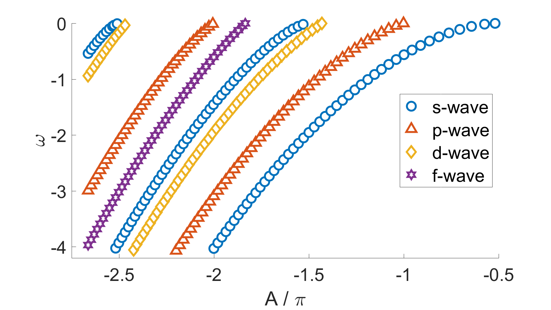
Figure 2: The spectrum of the square well potential [Eq. (54)] as a function of the universal parameter $A$ [Eq. (57)]. As $-A/\pi$ crosses an integer (half-integer) value, a new bound p-wave (s-wave) appears in the well. Higher order $l$ states appear progressively within these intervals. The nondimensional energy scale is fixed by setting the well size to $d=2$.

III Poles and Singularities with Periodic Driving

In this section we employ the methods presented in the previous sections to study a model system consisting of a spherically-symmetric square-well potential and a time-dependent periodic linear drive which acts outside of the well. Using the fundamental frequency of the periodic drive, $\Omega$, we can define the length and energy scales

$$d_{o}=\sqrt{2\hbar/m\Omega},\qquad E_{o}=\hbar\Omega/2,$$ (52)

and originally dimensional variables become nondimensional by rescaling according to

$$\vec{r}\to\vec{r}/d_{o},\qquad\vec{k}\to\vec{k}d_{o},\qquad t\to t\Omega/2,$$ (53)

after which we have explicitly $\hbar=m=1$ and the drive’s frequency in these units is $\Omega=2$. With a spherical square-well potential,

$$V_{{\rm int}}\left(\left|\vec{r}\right|\right)=\left\{\begin{array}[]{cc}{-V_{0},}&{\left|\vec{r}\right|<d}\\ {0}&{\left|\vec{r}\right|>d}\end{array}\right.$$ (54)

(where $d$ and $V_{0}$ are nondimensional, measured in the units of Eq. (52)), and the regular solution inside the well is a spherical Bessel function,

$$\phi_{\left\{k,l,m\right\}}\left(\vec{r},t\right)\propto e^{-i\left(\frac{1}{2}k^{2}-{V_{0}}\right)t}j_{l}\left(kr\right)Y_{l}^{m}.$$ (55)

In those units, we take the periodic force of Eq. (15) to be a simple harmonic drive with amplitude $F_{2}$,

$$F^{\pi}\left(t\right)=F_{2}\cos 2t,$$ (56)

regaining Eq. (8).

We define the well parameter

$$A=-\sqrt{2V_{0}d^{2}},$$ (57)

that is the single parameter that characterizes the square well nussenzveig1959poles . In Fig. 2 we show the spectrum of bound states of the time-independent square-well over a small range as function of the universal parameter $A/\pi$. The energy scale is obtained using Eq. (52), fixing $d=2$. It can be immediately seen from Eq. (57) that varying $\Omega$ is equivalent to leaving $A$ invariant while scaling both $V_{0}$ and $d$, as the energy and distance units are rescaled.

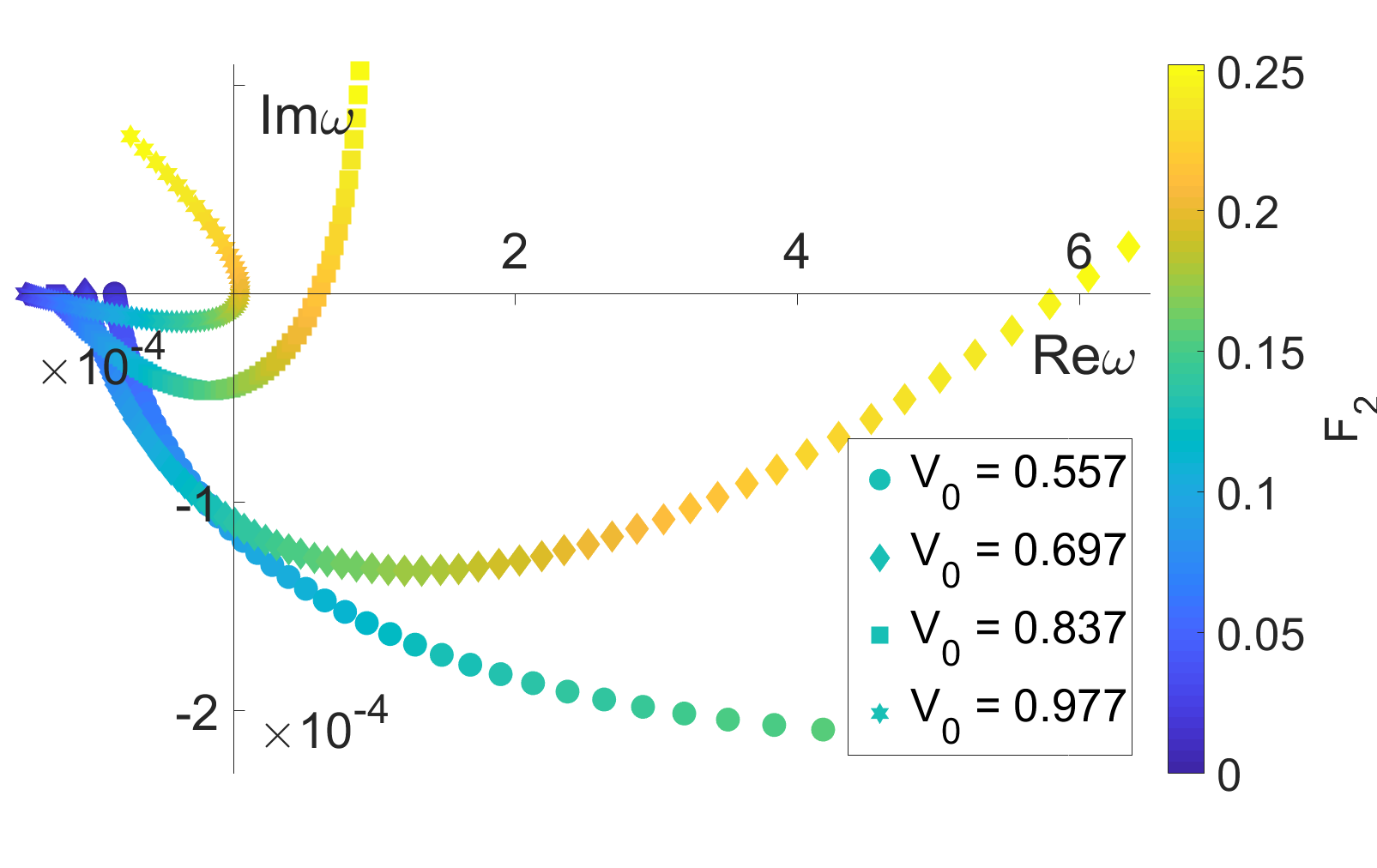
Figure 3: Complex $\omega$-space showing 4 resonances of the square-well potential [Eq. (54)] followed as a function of $F_{2}$ [Eq. (56)] by solving Eqs. (24)-(25), i.e., the drive is restricted to act outside the well (in contrast to Fig. 1). The well parameter of Eq. (57) is fixed at $-A/\pi\approx 0.504$, with $V_{0}$ taking 4 different values shown in the legend, $d$ being adjusted accordingly. Starting from the (single) loosely-bound s-wave state (see Fig. 2), the poles of the S-matrix correspond initially (while Im$\omega<0$) to the escape process (emission out of the well). The pole for $V_{0}=0.557$ crosses the real $\omega$-axis outside of the figure boundaries, at the critical parameters [Eq. (11)] $\bar{F}^{c}\approx 0.260$, $\bar{\omega}^{c}\approx 3.35\times 10^{-3}$ (see Fig. 6 to Fig. 8).

III.1 Driving a loosely bound s-wave

In this subsection we set $-A/\pi\approx 0.504$, i.e. the well is shallow with a single bound s-wave state close to threshold. We solve the problem by plugging the potential [Eq. (54)] into Eq. (25), i.e., the drive is restricted to act outside the well. This is in contrast to the results presented in Fig. 1, where the drive was solved for in all space. Choosing this form is motivated by the fact that for a general interaction potential, the problem cannot be solved exactly together with the periodic drive, and some sort of approximation is required. A possible choice [introduced in Eq. (1)] is to divide space into two regions where either the interaction or the periodic drive act. A further discussion and comparison of the two models will be presented in Sec. III.3.

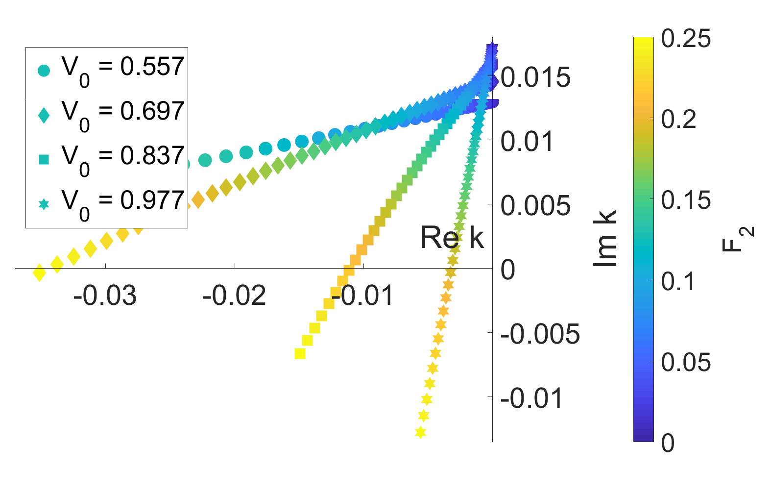
Figure 4: Complex $k$-space showing the value of $k_{0}$ at the poles of Fig. 3. The pole trajectories can be seen to lie almost along straight lines in this case (see however Fig. 14). The poles of the corresponding capture process (related by time-reversal invariance of the Hamiltonian) have mirror-imaged trajectories at the right half-plane (not shown). For each (capture or emission) pole of the S-matrix, there is also a zero at $-k$.

Figure 5: Absolute value of the matching coefficients of the solution [Eq. (26)], in the interior region ($a_{2n,l}$) and in the exterior region ($b_{2j,l_{1}}$), for the lowest pole Fig. 3 with $V_{0}=0.557$, at ${F}_{2}=0.03$. The superposition of (a small number of) components can be seen, both inside and outside the well, of decaying ($j\leq 0$) as well as travelling waves ($j\geq 1$).

Figure 3 shows the values of $\omega$ for the (initially) escape (radiating) pole followed by continuation from the s-wave bound state at $F_{2}=0$, at 4 different values of $V_{0}$ (with $A$ fixed). It can be seen that the crossing of the real $\omega$ axis is generic and can be realized at different values of the parameters. For low drive amplitude, the quasi-bound state’s decay rate grows quadratically (as can be inferred from a log-log plot, not shown), which is the expected perturbative result [Eq. (7)]. In the nonperturbative regime the decay rate is clearly nonmonotonous; for a strong enough drive it decreases and reaches 0, as the poles reach the real $\omega$-axis.

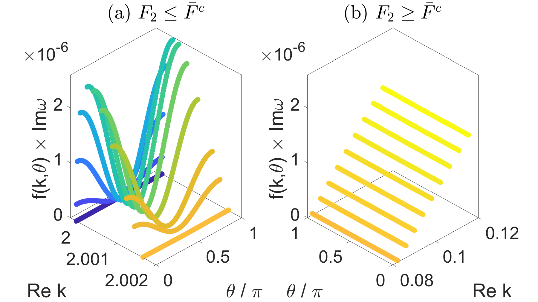
Figure 6: The leading order contribution to the the probability density $f(k,\theta)$ in spherical coordinates of momentum flux [see Eq. (44)], multiplied by (half) the rate of emission out of the well, plotted for increasing values of $F_{2}$, for the lowest pole in Fig. 3 with $V_{0}=0.557$. The curve colors (from dark blue to bright yellow) encode the value of $F_{2}$. (a) For $F_{2}$ up to the critical value $\bar{F}^{c}\approx 0.260$ the radiation is mostly p-wave in the $j=1$ channel. (b) At the critical value the distribution switches abruptly to the $j=0$ channel (mostly s-wave). The multiplication by the emission rate that goes through 0 makes the physical process smoothly decaying and then rising, despite the fact that the distribution $f(k,\theta)$ changes abruptly.

Figure 4 shows the momentum space values of $k_{0}$ for the same solutions, lying on nearly straight lines . The slope of the lines varies continuously with the parameters. The properties of the solutions were described at length in Sec. I, and we further discuss the parametric dependence in Sec. IV. Since in momentum space, the poles that start on the imaginary $k$-axis must cross the bisector of their quarter plane before reaching the Im$k=0$ line, in $\omega$ plane the poles follow a curved trajectory around the origin, crossing to Re$\omega>0$. This guarantees that after the critical point, the solutions that have switched roles (between capture and emission) remain valid – with Im$\omega\neq 0$ and one channel ($j=0$) that doesn’t decay asymptotically, as required by the continuity equation.

The superposition of different bound and diverging components can be seen in the solution coefficients of the expansion in Eq. (26), which are depicted in Fig. 5 for a particular state. The quasi-bound s-wave state which for $F_{2}=0$ would have its entire amplitude at $\left(n=0,l=0\right)$ and $\left(j=0,l_{1}=0\right)$, has developed a superposition of partial waves (here mostly outside of the well). The ‘checkerboard’ pattern is the result of the dipolar nature of the coupling, which conserves $\left(-1\right)^{n+l}$ [or $\left(-1\right)^{j+l_{1}}$], and can be used in practice to speed up the numerical calculations. Figure 6 shows the radiation pattern in the leading nondecaying channel for the lowest radiating pole of Fig. 3 with $V_{0}=0.557$. The joint probability density of the radiated waves given by $f(k,\theta)$ of Eq. (44) multiplied by Im$\omega$, is plotted at discrete steps of $F_{2}$ which determines the value of Re$k$. On the left, for $F_{2}$ lower than the critical value $\bar{F}^{c}\approx 0.260$, the radiation is an odd Legendre polynomial of $\cos\theta$ (mostly p-wave) in $j=1$ channels, with the flux initially increasing and then decreasing. On the right hand side, immediately after the pole crosses the real $\omega$ axis (at $\bar{\omega}^{c}\approx 3.35\times 10^{-3}$), the radiation abruptly collapses into the $j=0$ channels, composed mostly of s-waves (and other even harmonics), with the flux increasing as $F_{2}$ further increases.

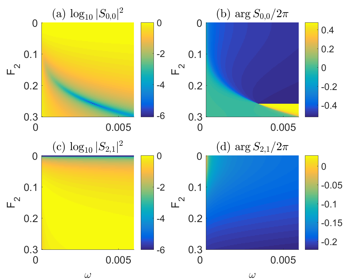
Figure 7: (a) The squared absolute value of the S-matrix element of the incoming s-wave ($|S_{0,0}|^{2}$), color coded on a logarithmic scale as function of $F_{2}$ and the real incoming wave energy $\omega$. $S_{0,0}$ vanishes at the value of $F_{2}$ and energy for which the pole lies on the real energy axis ($\bar{F}^{c}\approx 0.260$, $\bar{\omega}^{c}\approx 3.35\times 10^{-3}$, for the same pole as Fig. 6), with the finite grid size of the figure giving a small nonzero value. This corresponds to total absorption in this channel – all incoming waves are scattered into the other output channels. (b) The argument of the S-matrix element, ${\rm arg}\,S_{0,0}$, showing that a $2\pi$ phase is accumulated around the critical point in this parameter space. (c) The amplitude of outgoing p-waves in $j=1$ channel, given by $|S_{2,1}|^{2}$ that approaches unity near the critical point (in a logarithmic scale). (d) The argument ${\rm arg}\,S_{2,1}$, which shows no feature like that of panel (b).

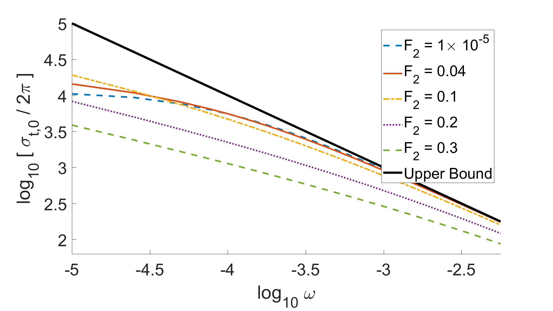
Figure 8: The base-10 logarithm of the total scattering cross sections divided by $2\pi$ [Eq. (49)], as a function of the real incoming wave energy $\omega$, for the input s-wave channel (which gives the scattering in the limit of slow particles). The parameters are identical to Fig. 7. The curves at several $F_{2}$ values, plotted on a log-log scale, show how for $F_{2}\to 0$ the scattering is predominantly elastic (with the $\omega\to 0$ dependence being that of $\sigma_{e,0}$, i.e. is energy-independent), and becoming increasingly dominated by the inelastic scattering ($\propto\omega^{-1/2}$). The cross section does not show any nonmonotonous features however – compare with Fig. 10 and Fig. 11.

Figure 7 shows some quantities of the S-matrix of a scattering formulation as a function of $F_{2}$ and the energy $\omega\ll 1$ of an incoming s-wave (which determines the limit of scattering of slow particles, see Sec. II.5). The parameters are the same as for the pole followed in Fig. 6. The critical point [defined in Eq. (11)] where the two complex conjugate poles (and zeros) of the S-matrix coincide on the real energy axis can be identified as at this point the S-matrix element $S_{0,0}$ vanishes (making the argument undefined), and a $2\pi$ phase is accumulated if going around this point in $(F_{2},\omega)$ parameter space. ${\rm arg}\,S_{0,0}$ is defined by continuity from $\omega\to 0$ for each fixed value of $F_{2}$. Along such a line for which $F_{2}<\bar{F}^{c}$ there is a sharp decrease of the argument as function of $\omega$, while for $F_{2}>\bar{F}^{c}$ there is a sharp rise. The S-matrix element $S_{2,1}$ of scattered p-waves in the $j=1$ channel approaches unit modulus (in a large region of the parameter plane). At the critical point there is total absorption of the incoming s-wave, and it is being radiated out as a (mostly) p-wave, with energy higher by at least a drive quantum.

In Fig. 8 the total scattering cross section is plotted for s-waves with $\omega\ll 1$. The features of scattering of slow particles discussed in Sec. II.6 (the energy-independent elastic scattering length and the $1/v$ law for inelastic scattering) hold, as can be deduced from an examination of the elastic and inelastic cross section curves (not shown). The total cross section changes its behaviour as a function of the drive amplitude – for $F_{2}\to 0$ the scattering is elastic, and it becomes increasingly inelastic as $F_{2}$ is increased. The cross section however is monotonous as a function of the energy (as is typical for an s-wave resonance) throughout the large variation of $F_{2}$. This is very different from the results of driving a bound p-wave state to be discussed in the next subsection.

III.2 Driving a deeper bound p-wave

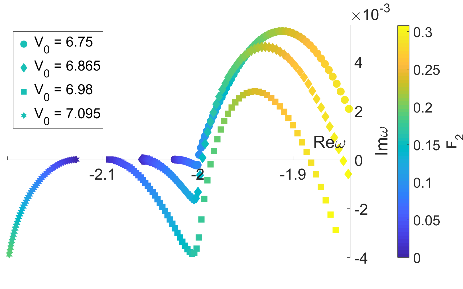
Figure 9: Complex $\omega$-space (as in Fig. 3) showing 4 resonances of the square-well potential for the well parameter fixed at $-A/\pi\approx 2.565$. Each being initially a p-wave bound state with energy $\omega(F_{2}=0)\lesssim-2$, at least $N\geq 2$ quanta of the external drive (of frequency $2$) must be absorbed in each radiating channel (Re$\omega+2j>0$, $j\geq 2$). Even as the three S-matrix poles which are pushed towards a larger quasi-energy cross to Re$\omega\geq-2$, the same channels ($j\geq 2$) are the only radiating ones, since the $j=1$ channel remains incoming and decaying. At the crossing of the real $\omega$-axis the solutions are singular in a similar manner to the near-threshold s-waves.

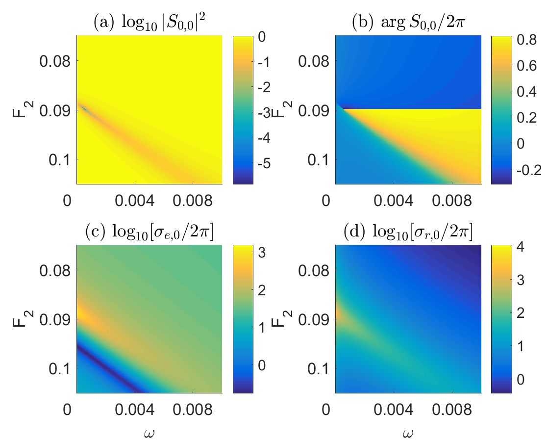
Figure 10: (a) As in Fig. 7, $|S_{0,0}|^{2}$ color coded on a logarithmic scale as function of $F_{2}$ and $\omega$, corresponding to the pole with $V_{0}=6.75$ in Fig. 9 (with $\bar{F}^{c}\approx 0.0898$, $\bar{\omega}^{c}\approx-1.9995$). (b) The argument of the S-matrix element, ${\rm arg}\,S_{0,0}$, showing a $2\pi$ phase jump, around $\bar{F}^{c}$ and $\omega\approx 5\times 10^{-4}$, which plausibly corresponds to an incoming s-wave completely transferred into the quasi-bound p-wave state by emitting a quantum of energy into the drive, and then being radiated as a p-wave, 2 quanta higher in energy. We note the different range of the argument as compared with Fig. 7, determined by the $\omega\to 0$ limit. (c) The base-10 logarithm of the elastic [Eq. (47)] and (d) the inelastic [Eq. (48)] cross sections divided by $2\pi$, for the input s-wave channel (in the limit of scattering of slow particles). Sharp features exist in the cross sections (more details are discernible in Fig. 11) in a relatively small range of $F_{2}$ and a large range of energy, to be contrasted with Fig. 8.

Figure 11: (a) The elastic, (b) inelastic, and (c) total scattering cross sections divided by $2\pi$ [Eqs. (47)-(49)], vs. the energy of the incoming wave (on a log-log plot), taken at a few values of $F_{2}$ around the critical value $\bar{F}^{c}\approx 0.0898$, for the same parameters as in Fig. 10. The nonmonotonous features of the cross sections as function of energy, and the strong alteration of the curves as function of $F_{2}$ are evident, as well as the $\omega\to 0$ dependence of $\sigma_{e,0}$ (energy-independent) and of $\sigma_{r,0}$ ($\propto\omega^{-1/2}$), as required by the slow-particle scattering limits.

In this subsection we set $-A/\pi\approx 2.565$ and focus on a p-wave (with magnetic quantum number $m=0$) whose binding energy (for $F_{2}=0$) is a little larger than $2$ – absorption of two quanta is necessary (for $F_{2}\ll 1$) to emit outgoing waves. The same equations are solved as in the previous subsection. Figure 9 shows the values of $\omega$ for four poles followed by continuation. Three of those poles cross towards Re$\omega>-2$ while there is one pole that is pushed towards negative energies. An exceptional point, discussed further in Sec. IV, separates the poles going left and right. As in the previous subsection, as the poles in the lower half plane cross the line Re$\omega=-2$, the channels whose energy becomes positive (and for that could be termed ‘open’) remain in fact asymptotically decaying (and in fact incoming) so the radiation pattern does not show a qualitative change.

As the poles cross to the upper half $\omega$-plane, the solutions change their nature abruptly and they are singular on the real energy line. The pole trajectories in momentum space will be shown in Sec. IV and present a nontrivial behavior. The radiation pattern (not shown) presents similar features to that of Fig. 6 (with the required modifications of the momentum values and the distribution shape).

Figures 10-11 show the characteristics of a scattering setup with slow particles. The limiting low energy behaviors of the cross sections, discussed in Sec. II.6, are clearly visible – an energy independent elastic cross section and the $1/v$ law for the inelastic scattering cross section. Sharp features and nonmonotonicity of the scattering as function of $F_{2}$ and in particular of $\omega$ are present, resembling shape- and Fano-resonances (we return to this point briefly in Sec. IV). The presence of the pole at $\bar{\omega}^{c}\approx-1.9995$ suggests that at the critical point, an incoming s-wave with low energy $\omega=\bar{\omega}^{c}+2$ emits one quantum of energy into the drive and is completely captured into the (long-lived) bound state, only to be radiated as a (mostly) p-wave after absorbing two quanta from the drive.

III.3 Approximations

We now discuss the truncation of the potential introduced in Eq. (25) that we repeat here,

$$\begin{array}[]{cc}&V_{{\rm in}}^{(1)}\left(\vec{r},t\right)=\left[V_{{\rm int}}\left(r\right)\right]\Theta(d-r),\\ \\ &V_{{\rm out}}^{(1)}\left(\vec{r},t\right)=\left[-\ddot{\vec{F}}\left(t\right)\cdot\vec{r}+V_{F}\left(t\right)\right]\Theta(r-d),\end{array}$$ (58)

which corresponds to truncating the axial drive inside the well. The solutions presented in the subsections III.1-III.2 were all obtained using this form of the potential. The solutions presented in Fig. 1 do not employ this truncation, but rather solve the full problem with

$$\begin{array}[]{cc}&V_{{\rm in}}^{(2)}\left(\vec{r},t\right)=\left[V_{{\rm int}}\left(r\right)-\ddot{\vec{F}}\left(t\right)\cdot\vec{r}+V_{F}\left(t\right)\right]\Theta(d-r),\\ \\ &V_{{\rm out}}^{(2)}\left(\vec{r},t\right)=\left[-\ddot{\vec{F}}\left(t\right)\cdot\vec{r}+V_{F}\left(t\right)\right]\Theta(r-d),\end{array}$$ (59)

with the parameters for Fig. 1 being

$$-A/\pi\approx 0.504,\qquad V_{0}=1.977.$$ (60)

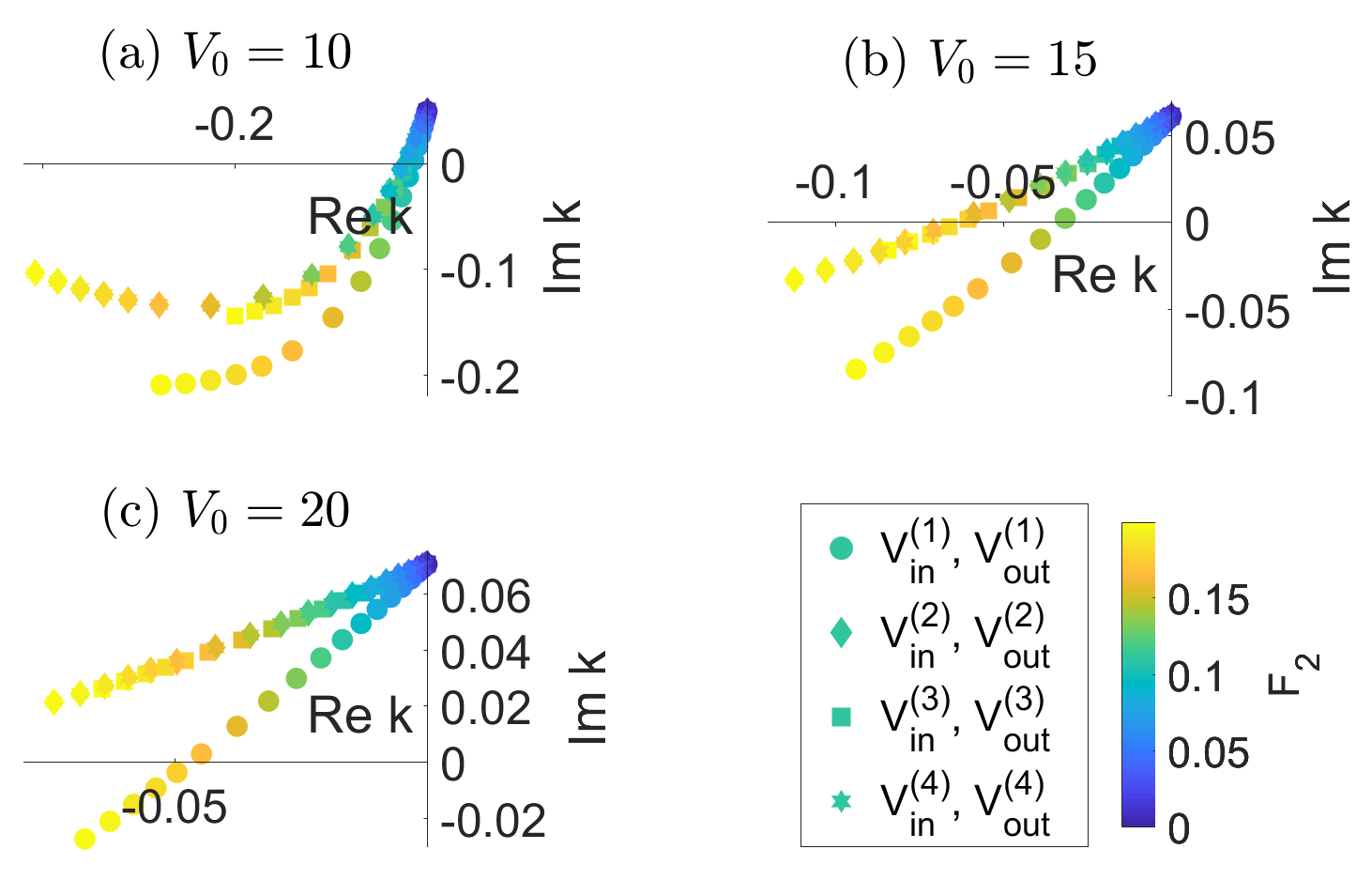
Figure 12: Complex $k$-space comparing poles solved using different potentials defined in Sec. III.3, studying the approximation involved in truncating the drive inside the well, and also the effect of $V_{F}$ of Eq. (6). See the text for the analysis.

For $V_{{\rm in}}^{(2)}$ of Eq. (59), the wavefunctions in the interior region become time dependent and have to be Fourier expanded as in the exterior region (making the matrices $C$ and $F$ of Eq. (39) nondiagonal). As noted above, $V_{F}(t)$ is the result of taking Eq. (2) as the physical starting point (an oscillating center of the potential). $V_{F}$ then cancels the prefactor in Eq. (14),

$$e^{-i\int^{t}\frac{1}{2}\dot{F}^{2}(t^{\prime})dt^{\prime}},$$ (61)

that would otherwise multiply the wavefunction. If Eq. (5) is the physical potential (a static potential with an external, periodically modulated linear force), we can define $V_{{\rm in}}^{(3,4)}$ and $V_{{\rm out}}^{(3,4)}$ to be equal to $V_{{\rm in}}^{(1,2)}$ and $V_{{\rm out}}^{(1,2)}$ with $V_{F}(t)$ set to 0. Then the solutions have to be matched including the term of Eq. (61) that shifts the quasi-energy and modifies also the Fourier expansion.

Figures 12-13 show the pole trajectories for a near-threshold s-wave bound state of a well with $-A/\pi\approx 2.5037$, solved for three increasing different well depth $V_{0}$, and for each value, comparing the four potentials $V_{{\rm in}}^{(p)}+V_{{\rm out}}^{(p)}$ with $p=1,2,3,4$.

The most notable result is that the singularities studied in this work exist with all of the studied forms of the potential. They are the result of tunneling and interference, and since they exist with $p=3$, they are not hindered by the possibility to directly couple to the continuum by absorbing energy within the well. The solution with $p=1$ approximates the potential with $p=2$, that can be considered as the ‘true’ potential in a realization that starts from Eq. (2), although there are noticeable differences in the slopes in momentum space, which lead to some deviations in $\omega$ space as well. This approximation depends on the norm of the wavefunction in the exterior region (which is subject to drive). The poles with $p=3$ and $p=4$ are closer to each other (for deeper well depths) in energy space because of the importance of $V_{F}$, although in momentum space they do not coincide – in fact the poles for $p=2$ and $p=4$ coincide exactly in momentum space, because when $V_{F}$ appears both within and outside the well, its value does not enter the momentum matching.

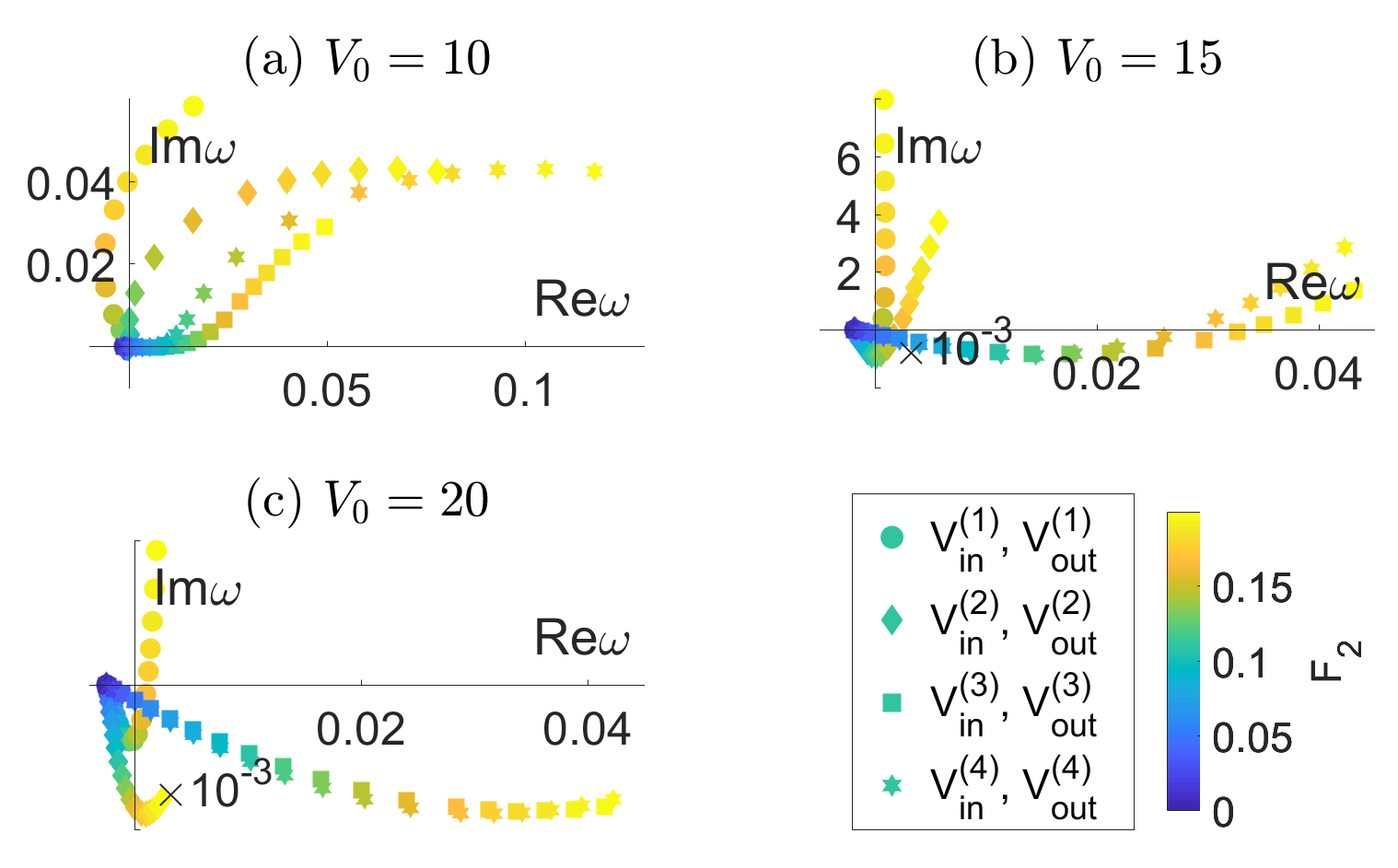
Figure 13: Complex $\omega$-space for the poles of Fig. 12 solved using different potentials (see text for details).

We note the difference between the expansion presented in the previous sections and the well known Floquet formalism for treating periodic Hamiltonians PhysRev.138.B979 ; PhysRevA.7.2203 ; tannor2007introduction , or time-dependent perturbation theory RevModPhys.44.602 . The periodicity of the Hamiltonian allows defining an extended Hilbert space in position and time, that can be spanned by a set of spatially orthogonal wavefunctions and a Fourier basis for time-periodic functions. The current expansion however, employs exact wavefunctions (at least asymptotically), that vary with $\omega$ and are not separable in time and space, in contrast to an expansion using a fixed separable basis that would typically require significantly more basis functions. The connection to the physical solutions is transparent and the explicit use of analytic wavefunctions in each region gives access to details of the spectrum which may be hard to locate otherwise, and in particular Quantum Defect Theory (QDT), discussed in Sec. I, can be used for the expansion of wavefunctions in the interior region. Our approach is nonperturbative in both potentials, but neglects the effect of either potential in some region of space and the obtained solutions can be considered, if necessary, as a starting point for an expansion that will correct for the neglected contributions.

Finally we note that the presented expansion and numerical results have been verified by using two different numerical routines in two different programming languages (Matlab and Mathematica), and then directly by plugging the explicit wavefunction into the time-dependent Schrödinger equation and verifying the vanishing of both sides of the equation, to the numerical precision possible in the calculation and according to the truncated components.

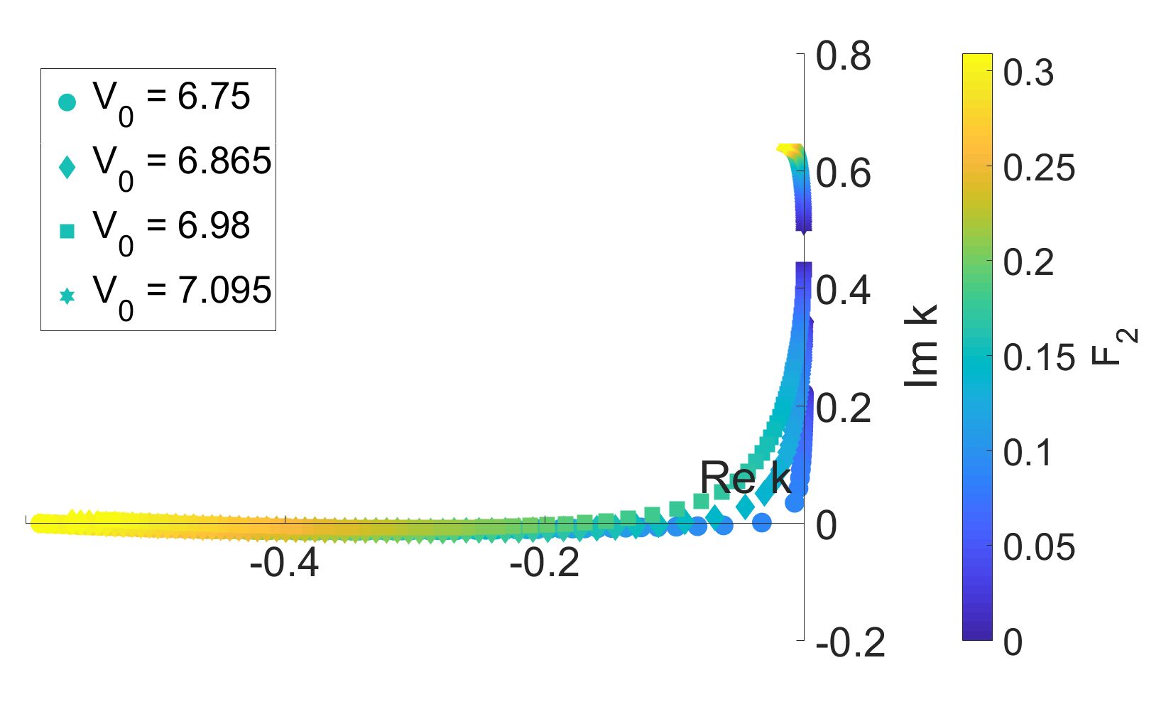
Figure 14: Complex $k$-space showing the value of $k_{2}$ at the poles of Fig. 9. The pole trajectories can be seen to deviate significantly from the almost straight lines seen (for different parameters) in Fig. 4. A further study is required in order to explain this and possibly relate it to ‘resonance interaction’ and to the nearby exceptional point (see the text and Fig. 15).

IV Outlook

The momentum space values of $k_{2}$ for the poles followed in Sec. III.2 (Fig. 9) are shown in Fig. 14. In contrast to Fig. 4 of Sec. III.1, here the pole trajectories in momentum space deviate significantly from straight lines. This may correspond to the proximity of other poles (‘resonance interaction’), and to the existence of the exceptional point nearby rotter2004influence ; heiss2012physics , discussed below.

Figure 15 compares two scenarios for the pole trajectories in complex momentum and energy planes when varying $V_{0}$ continuously. In panels (a) and (b), a smooth rotation of the pole trajectories can be seen as their slope changes continuously with $V_{0}$, going through a point which plausibly shows an interchange of the poles which become the capture and emission poles (that are indistinguishable here at $F_{2}=0$, but possibly could be distinguished with a Floquet invariant like the Krein signature Yakubovich ). In panels (c) and (d), $A$ is fixed as in Fig. 14, and $V_{0}$ is varied in small range around the point at which the pole trajectories of Fig. 14 seem to ‘branch’. The existence of an exceptional point is clearly seen, where two bound states for $F_{2}=0$ coincide in energy (mod 2), around which the parametric dependence appears to be nonanalytic. An initial study indicates an entire line of exceptional points that emanates from this point in $(V_{0},F_{2})$ parameter space. Further study is required in order to check whether an exceptional point can be followed up to the real $\omega$-axis as the Floquet poles studied above, whence it may share further similarities with a spectral singularity of scattering with a real energy. As discussed in Sec. I, the role of exceptional points in non-Hermitian (open) systems is attracting increasing attention, and new effects are being actively explored.

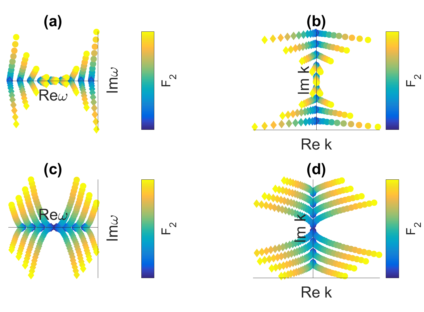
Figure 15: (a) Complex $\omega$-space and (b) complex $k$-plane for a series of poles with a fixed value of $A$, as in Fig. 3, and $V_{0}$ varied between $1.15$ and $1.3$ (the 9 nearly-straight lines starting a adjacent values of $\omega$ or ${\rm Im}k$ respectively). The axis markings and the scale of $F_{2}\ll 1$ (given by the color code) have been removed for clarity. A smooth rotation of the two pole curves (in both energy and momentum planes) can be seen as function of $V_{0}$. This is to be contrasted with the seemingly nonanalytic point visible in (c) complex $\omega$-space and (d) complex $k$-plane for a series of p-wave poles with $A$ fixed as in Fig. 9 and Fig. 14, and $V_{0}\in[7.078,7.091]$. Here it is a Floquet-induced (time-independent) exceptional point, where the p-wave bound state with energy $\omega\approx-2.125$ coincides in energy (mod 2) with the s-wave of $\omega\approx-0.125$, for $V_{0}\approx 7.09$. A further study is required to confirm a possible line of exceptional points passing through this point.

The cross sections in Fig. 11 show features resembling shape- and Fano-resonances, which are important in atomic and also nanoscale structures flach2003fano ; miroshnichenko2010fano ; ott2013lorentz (with the distinction that here the scattering is inelastic, and the potential is time-dependent and non-central, both of those aspects playing an important role). As discussed in Sec. II.6, the two linearly indepenednt solutions of a power law potential $-C/r^{\alpha}$ with $\alpha>3$, are analytic in complex energy and momentum planes. Hence, when applying the expansion of the current work to match such wavefunctions in the interior region with the driven particle wavefunctions in the exterior region, no nonanalyticity is introduced in the entire $k$-plane (at any fixed $r\neq d$). Therefore, following the poles of the driven problem in $k$-plane for such a potential should be possible (a-priori) as shown here for a finite range potential. A further study of the possibility to tailor scattering and resonances using Floquet driving, in particular of atomic systems ZeroFloquet , is a promising direction to apply the techniques developed in this work. Indeed, the singular points analyzed in the current work can be found in an explicit calculation employing QDT with the polarization interaction ($\alpha=4$) of a cotrapped ion-atom system unpublished . More broadly, Floquet driven systems are often analyzed in terms of a time-independent, effective approximation. Our results show a scenario where accounting for the time-dependent nature of the drive is essential, and the implications to many-body Floquet systems della2013spectral ; lindner2011floquet ; goldman2014periodically ; mitrano2016possible present an intriguing future direction to explore.

Appendix A Expansion of linearly-driven cylindrical waves in spherical waves

In the following we will use a representation of the spherical Hankel function of the first kind as an integral over cylindrical waves DanosMaximon ; bostrom1991transformation in the form

$$h_{l}^{\left(1\right)}\left(kr\right)P_{l}^{m}\left(\cos\theta\right)e^{im\varphi}=\int_{C^{(1)}}d\alpha\sin\alpha\frac{1}{2}\left(-i\right)^{l-m}P_{l}^{m}\left(\cos\alpha\right)\chi_{m}^{\left(1\right)}\left(\vec{r};k,\alpha\right)$$ (62)

where $P_{l}^{m}$ are the associated Legendre polynomials and the directed contour of integration $C^{(1)}$ lies in complex $\alpha$-plane. For $k$ with a positive imaginary part we must take $C^{(1)}=\pi/2+i\left(\infty,-\infty\right)$, on which $\cos\alpha\in i\left(\infty,-\infty\right)$, and $\sin\alpha\in\left(0,\infty\right)$. Then $h_{l}^{\left(1\right)}\left(kr\right)$ decays asymptotically as $e^{-({\rm Im}k)r}/r$ (the integral which gives $h_{l}^{\left(1\right)}\left(kr\right)$ is well defined for any $\rho>0$, and decays for $r\to\infty$, which is just what is required for the validity of the solution). For $k$ real and positive the contour of integration is given by $C^{(1)}=i\left(\infty,0\right)+\left[0,\pi\right]+\left\{\pi+i\left(0,-\infty\right)\right\}$, on which $\cos\alpha\in\left(\infty,-\infty\right)$, and $\rm{Im}\sin\alpha\geq 0$. For any value of $k$, we have similarly to Eq. (62)

$$j_{l}\left(kr\right)P_{l}^{m}\left(\cos\theta\right)e^{im\varphi}=\int_{\left[0,\pi\right]}d\alpha\sin\alpha\frac{1}{2}\left(-i\right)^{l-m}P_{l}^{m}\left(\cos\alpha\right)\chi_{m}^{\left(J\right)}\left(\vec{r};k,\alpha\right),$$ (63)

where $j_{l}$ is a spherical Bessel function. Writing $h_{l}^{\left(2\right)}=2j_{l}-h_{l}^{\left(1\right)}$, and using eqjlexpansion and the fact that the $l,m$-dependent coefficients in Eqs. (62)-(63) are identical, we get an expression identical in form to Eq. (62), with the outgoing waves replaced by incoming waves $h_{l}^{\left(2\right)}$, and a contour $C^{(2)}$. A similar derivation can be repeated in the lower half of complex $k$ plane, making the expansion valid for every complex $k$ (which also follows by analytic continuation).

The proof of Eq. (21) proceeds by using Eq. (18) to write

$$\begin{array}[]{l}{e^{i\dot{F}^{\pi}\left(t\right)z}\int_{C^{(a)}}d\alpha\sin\alpha\chi_{m}^{\left(a\right)}\left(\vec{r};k_{2j},\alpha\right)b_{{2j}}^{\left(a\right)}\left(\alpha\right)e^{-iF^{\pi}\left(t\right)k_{2j}\cos\alpha}}\\ \\ \qquad{=e^{i\dot{F}^{\pi}\left(t\right)z}\int_{C^{(a)}}d\alpha\sin\alpha\chi_{m}^{\left(a\right)}\left(\vec{r};k_{2j},\alpha\right)\sum_{l_{1}}b_{2j,l_{1}}P_{l_{1}}\left(\cos\alpha\right)\sum_{l_{2}}\left(-i\right)^{l_{2}}\left(2l_{2}+1\right)j_{l_{2}}\left(F^{\pi}\left(t\right)k_{2j}\right)P_{l_{2}}\left(\cos\alpha\right)}\\ \\ \qquad{=e^{i\dot{F}^{\pi}\left(t\right)z}\sum_{l_{1},l_{2}}b_{2j,l_{1}}\left(-i\right)^{l_{2}}\left(2l_{2}+1\right)j_{l_{2}}\left(F^{\pi}\left(t\right)k_{2j}\right)\sum_{l_{3}}W\left(P_{l_{1}},P_{l_{2}},P_{l_{3}}^{m}\right)\int_{C^{(a)}}d\alpha\sin\alpha\chi_{m}^{\left(a\right)}\left(\vec{r};k_{2j},\alpha\right)P_{l_{3}}^{m}\left(\cos\alpha\right)}\\ \\ \qquad{=e^{i\dot{F}^{\pi}\left(t\right)z}\sum_{l_{1},l_{2}}b_{2j,l_{1}}j_{l_{2}}\left(F^{\pi}\left(t\right)k_{2j}\right)\sum_{l_{3}}c_{l_{1},l_{2},l_{3}}h_{l_{3}}^{\left(a\right)}\left(k_{2j}r\right)P_{l_{3}}^{m}\left(\cos\theta\right)e^{im\varphi}}\\ \\ \qquad{=\sum_{l_{4}}i^{l_{4}}\left(2l_{4}+1\right)j_{l_{4}}\left(\dot{F}^{\pi}\left(t\right)r\right)P_{l_{4}}\left(\cos\theta\right)\sum_{l_{1},l_{2}}b_{2j,l_{1}}j_{l_{2}}\left(F^{\pi}\left(t\right)k_{2j}\right)\sum_{l_{3}}c_{l_{1},l_{2},l_{3}}h_{l_{3}}^{\left(a\right)}\left(k_{2j}r\right)P_{l_{3}}^{m}\left(\cos\theta\right)e^{im\varphi}}\\ \\ \qquad{=\sum_{l_{1},l_{2},l_{3},l_{4}}b_{2j,l_{1}}j_{l_{2}}\left(F^{\pi}\left(t\right)k_{2j}\right)j_{l_{4}}\left(\dot{F}^{\pi}\left(t\right)r\right)h_{l_{3}}^{\left(a\right)}\left(k_{2j}r\right)\sum_{l}c_{l_{1},l_{2},l_{3},l_{4},l}Y_{l}^{m}\left(\theta,\varphi\right)}\end{array}$$ (64)

where the multiplicative factors $e^{-i\frac{1}{2}k_{2j}^{2}t}$, $N_{2j,l_{1}}^{m}$, and $S_{2j,l_{1}}^{\left(a\right)}$ have been omitted for simplicity, and by using the definition of $R_{2j,l_{1},l}^{\left(a\right)}\left(r,t\right)$ given in Eq. (22), Eq. (64) results in Eq. (21). In the derivation of Eq. (64), the plane-wave expansion in terms of spherical Bessel functions has been used (twice), the coefficients of expansion of a product of two (associated) Legendre polynomials (which can be written using Wigner 3-j symbols) are defined by

$$W\left(P_{l_{1}}^{m_{1}},P_{l_{2}}^{m_{2}},P_{l_{3}}^{m_{3}}\right)=\left[2\left(l_{3}+m_{3}\right)!/\left(\left(2l_{3}+1\right)\left(l_{3}-m_{3}\right)!\right)\right]^{-1}\int_{-1}^{1}P_{l_{1}}^{m_{1}}\left(w\right)P_{l_{2}}^{m_{2}}\left(w\right)P_{l_{3}}^{m_{3}}\left(w\right)dw,$$ (65)

the coefficients $c_{l_{1},l_{2},l_{3}}$ are obtained using Eq. (62) and Eq. (65) and given by

$$c_{l_{1},l_{2},l_{3}}=2\left(2l_{2}+1\right)\left(-i\right)^{l_{2}}i^{l_{3}-m}W\left(P_{l_{1}},P_{l_{2}},P_{l_{3}}^{m}\right),$$ (66)

and the coefficients $c_{l_{1},l_{2},l_{3},l_{4},l}$ are similarly

$$c_{l_{1},l_{2},l_{3},l_{4},l}=c_{l_{1},l_{2},l_{3}}\left(2l_{4}+1\right)i^{l_{4}}W\left(P_{l_{3}}^{m},P_{l_{4}},P_{l}^{m}\right)/N_{l}^{m},$$ (67)

with the definitions

$$Y_{l}^{m}\left(\theta,\varphi\right)=N_{l}^{m}P_{l}^{m}\left(\cos\theta\right)e^{im\varphi},\qquad\qquad N_{l}^{m}=(-1)^{m}\sqrt{\left(2l+1\right)/4\pi}\sqrt{\left(l-m\right)!/\left(l+m\right)!}.$$ (68)

Appendix B The expectation value of tensor operators

In this appendix we give explicitly the expansion of integrals which are required in order to calculate expectation values of general tensor operators, in the Floquet eigensolutions of Sec. II.2. For simplicity we treat here only the most useful case of axially symmetric wavefunctions, with $m=0$ (no $\varphi$ dependence). Using the notation of Eq. (50), we start by writing the $\pi$-periodic part of the wavefunction in the form

$$\phi^{\pi}\left(\vec{r}\right)=\sum_{n,l}a_{2n,l}e^{-i2nt}\frac{1}{r}u_{2n,l}\left(r\right)Y_{l}^{0},$$ (69)

which corresponds to the expansion in Eq. (26) of wavefunctions in the interior region. For such wavefunctions, we define the (unnormalized) expectation value in the interior region of a purely radial operator $\mathcal{O}\left(r\right)$,

$$\mathfrak{I}_{0}\left[\mathcal{O}\left(r\right)\right]\equiv\int d^{3}\vec{r}\left|\phi^{\pi}\left(\vec{r},t\right)\right|^{2}\mathcal{O}\left(r\right)=\sum_{\left(n,l\right),\left(n^{\prime},l^{\prime}\right)}\delta_{l,l^{\prime}}e^{2i\left(n-n^{\prime}\right)t}a_{2n,l}^{*}a_{2n^{\prime},l^{\prime}}\int dr\left[u_{2n,l}\right]^{*}\mathcal{O}\left(r\right)u_{2n^{\prime},l^{\prime}}.$$ (70)

The above expression can be rewritten as

$$\mathfrak{I}_{0}\left[\mathcal{O}\left(r\right)\right]=\sum_{l}I_{l,l}\left[\mathcal{O}\left(r\right)\right],$$ (71)

where we have defined for convenience the functional [symmetric under the exchange $\left(n,l\right)\leftrightarrow\left(n^{\prime},l^{\prime}\right)$]

$${I}_{l,l^{\prime}}\left[\mathcal{O}\left(r\right)\right]=\sum_{n\leq n^{\prime}}\left(2-\delta_{n,n^{\prime}}\right)\,{\rm Re}\left\{e^{2i\left(n-n^{\prime}\right)t}a_{2n,l}^{*}a_{2n^{\prime},l^{\prime}}\int dr\left[u_{2n,l}\right]^{*}\mathcal{O}\left(r\right)u_{2n^{\prime},l^{\prime}}\right\},$$ (72)

with the summation taken over pairs of states enumerated by $\left\{\left(n,l\right),\left(n^{\prime},l^{\prime}\right)\right\}$ with fixed $l$ and $l^{\prime}$ obeying $n\leq n^{\prime}$.

For example, the normalization integral calculated for any time (see App. C) can be written as

$$\mathfrak{I}_{0}\left[\hat{1}\right]=\sum_{l}I_{l,l}\left[\hat{1}\right],$$ (73)

with $\hat{1}$ the identity operator. Any other expectation value must then be divided by the value of this normalization integral. Similarly, the expectation value of the squared angular momentum operator $\vec{L}^{2}$ is given by

$$\mathfrak{I}_{0}\left[\vec{L}^{2}\right]=\sum_{l}l\left(l+1\right)I_{l,l}\left[\hat{1}\right].$$ (74)

For an operator of a general radial part multiplied by the position vector, $\mathcal{O}\left(r\right)\vec{r}$, only the Cartesian $z$-component survives the integral (for axially symmetric wavefunctions), and we can write using $z/r=\cos\theta$

$$\mathfrak{I}_{1}\left[\mathcal{O}\left(r\right)\vec{r}\,\right]=\int d^{3}\vec{r}\left|\phi^{\pi}\left(\vec{r},t\right)\right|^{2}\mathcal{O}\left(r\right)\vec{r}=\hat{z}\sum_{\left(n,l\right),\left(n^{\prime},l^{\prime}\right)}p_{l,l^{\prime}}e^{2i\left(n-n^{\prime}\right)t}a_{2n,l}^{*}a_{2n^{\prime},l^{\prime}}\int dr\left[u_{2n,l}\right]^{*}\mathcal{O}\left(r\right)r\,u_{2n^{\prime},l^{\prime}}\,$$ (75)

with the coefficients being

$$p_{l,l^{\prime}}=2\pi N_{l}^{0}N_{l^{\prime}}^{0}\int d\theta\sin\theta\cos\theta P_{l}\left(\cos\theta\right)P_{l^{\prime}}\left(\cos\theta\right).$$ (76)

Using the fact that $p_{l,l^{\prime}}=p_{l^{\prime},l}$ and since nonzero terms will have $\left|l-l^{\prime}\right|=1$, we find

$$\mathfrak{I}_{1}\left[\mathcal{O}\left(r\right)\vec{r}\,\right]=\hat{z}\sum_{l}p_{l,l+1}\left(I_{l,l+1}\left[\mathcal{O}\left(r\right)r\right]+I_{l+1,l}\left[\mathcal{O}\left(r\right)r\right]\right).$$ (77)

For an operator with a general radial part multiplied by a bilinear combination of $\vec{r}$ components, $\mathcal{O}\left(r\right)\vec{r}_{\alpha}\vec{r}_{\beta}$, where $\alpha,\beta\in\left\{x,y,z\right\}$, only the diagonal terms with $\alpha=\beta$ survive the integration (for $m=0$), with the result

$$\mathfrak{I}_{2}\left[\mathcal{O}\left(r\right)\vec{r}_{\alpha}\vec{r}_{\beta}\right]=\delta_{\alpha,\beta}\sum_{l,l^{\prime}}q_{\alpha,l,l^{\prime}}I_{l,l^{\prime}}\left[\mathcal{O}\left(r\right)r^{2}\right],$$ (78)

where

$$q_{\alpha,l,l^{\prime}}=2\pi N_{l}^{0}N_{l^{\prime}}^{0}\int d\theta\sin\theta\left[\cos^{2}\theta\delta_{\alpha,z}+\frac{1}{2}\sin^{2}\theta\left(\delta_{\alpha,x}+\delta_{\alpha,y}\right)\right]P_{l}\left(\cos\theta\right)P_{l^{\prime}}\left(\cos\theta\right).$$ (79)

In all of the above expressions, ${I}_{l,l^{\prime}}\left[\mathcal{O}\left(r\right)\right]$ as defined in Eq. (72) is valid in the interior region. To get the complete result for expectation values in whole space, the integration over the exterior region must be added, where the wavefunctions are expanded differently in Eq. (26). In this case, Eq. (69) is to be replaced by

$$\phi^{\pi}\left(\vec{r},t\right)=\sum_{j,l_{1}}b_{2j,l_{1}}e^{-i2jt}\sum_{l}\frac{1}{r}u_{2j,l_{1},l}^{\pi}\left(r,t\right)Y_{l}^{0},$$ (80)

and accordingly, Eq. (72) becomes in the exterior region

$${I}_{l,l^{\prime}}\left[\mathcal{O}\left(r\right)\right]=\sum_{\left(j,l_{1}\right),\left(j^{\prime},l_{1}^{\prime}\right)}e^{2i\left(j-j^{\prime}\right)t}b_{2j,l_{1}}^{*}b_{2j^{\prime},l_{1}^{\prime}}\int dr\left[u_{2j,l_{1},l}^{\pi}\right]^{*}\mathcal{O}\left(r\right)u_{2j^{\prime},l_{1}^{\prime},l^{\prime}}^{\pi},$$ (81)

with the summation taken over pairs of states enumerated by $\left\{\left(j,l_{1},l\right),\left(j^{\prime},l_{1}^{\prime},l^{\prime}\right)\right\}$ with fixed $l$ and $l^{\prime}$. Finally, we note that in the above expressions, the imaginary part of the energy has been omitted – it gives an exponential envelope of the decay or formation rate of the quasi-bound state. Moreover, all integrals can be performed only on the square-integrable part of the wavefunction, with the nonnormalizable traveling waves omitted from the sums above, in accordance with the interpretation that these belong to the inaccessible part of the Hilbert space.

Appendix C Normalization of the wavefunction

The expectation value of any time-independent (or $\pi$-periodic) operator is $\pi$-periodic for the Floquet eigenstates, possibly with an exponential envelope for complex $\omega$. The normalization integral is not constant in time but rather $\pi$-periodic because the relative weight of the nonnormalizable components oscillates in time (as they are emitted and reflected back during a period of the drive). In order to calculate an expectation value of an operator (determined by the bound components), its integral must be divided by the squared norm, both of which being $\pi$-periodic functions that can be calculated using App. B (after which averaging is possible). The normalization in the interior region can be obtained without explicitly performing the integration, directly from the wavefunctions and their gradients at the matching point. This can be useful especially when the interior wavefunctions are not explicitly known close to the origin, but rather are determined within a QDT formulation Seaton1983 ; Gao2008 ; idziaszek2011multichannel ; PhysRevA.84.042703 ; PhysRevA.87.032706 . The projection of two eigenfunctions $\phi_{1}$ and $\phi_{2}$ of the interior Hamiltonian with energies $\varepsilon_{1}$ and $\varepsilon_{2}$ correspondingly, is shown in App. D to be

$$2\,{\rm Re}\int_{0}^{d}\phi_{1}^{*}\phi_{2}r^{2}dr=\left(\varepsilon_{1}-\varepsilon_{2}\right)^{-1}{\rm Re}\left.\left\{u_{1}^{*}u_{2}{{{}^{\prime}}}-u_{2}^{*}u_{1}{{{}^{\prime}}}\right\}\right|_{d},$$ (82)

where $u_{1}{{}^{\prime}}\equiv\partial_{r}u_{1}$, and $\varepsilon_{1}$, $\varepsilon_{2}$ are assumed to have equal imaginary parts. The left-hand side of Eq. (82) gives the integrals required for the normalization, with the factor of 2 relevant for the off-diagonal projections (when $\phi_{1}\neq\phi_{2}$). In the limit of $\phi_{1}\to\phi_{2}$ we have for the diagonal normalization terms

$$\int_{0}^{d}\left|\phi_{1}\right|^{2}r^{2}dr=\frac{1}{2}\mathop{\lim}\limits_{\varepsilon_{1}\to\varepsilon_{2}}\left(\varepsilon_{1}-\varepsilon_{2}\right)^{-1}\left.\left[u_{1}^{*}u_{2}{{{}^{\prime}}}-u_{2}^{*}u_{1}{{{}^{\prime}}}\right]\right|_{d}.$$ (83)

Appendix D The projection of two eigenfunctions of the internal Hamiltonian

In order to derive Eq. (82), let $\varepsilon_{1},\varepsilon_{2}$ be the (possibly complex) energies of two complex eigenfunctions $\phi_{1},\phi_{2}$ of the interior Hamiltonian $H_{\rm in}=-\frac{1}{2}\nabla^{2}+V_{\rm in}$. For the projection of the two within the interior region, we can write

$$0=\left\langle\phi_{2}\left|\left(H_{\rm in}-\varepsilon_{1}\right)\left|\phi_{1}\right.\right.\right\rangle-\left\langle\phi_{1}\left|\left(H_{\rm in}-\varepsilon_{2}\right)\left|\phi_{2}\right.\right.\right\rangle.$$ (84)

By canceling the potential energy terms, we get after rearranging the kinetic terms and terminating the integration at an arbitrary point $d$ (which is allowed since the equality above holds identically in space),

$$\begin{array}[]{l}{\int_{0}^{d}\left(\varepsilon_{1}\phi_{2}^{*}\phi_{1}-\varepsilon_{2}\phi_{1}^{*}\phi_{2}\right)r^{2}dr=-\frac{1}{2}\int_{0}^{d}\left(u_{2}^{*}\partial_{r}^{2}u_{1}-u_{1}^{*}\partial_{r}^{2}u_{2}\right)dr}\\ \\ {\qquad=-\frac{1}{2}\left[\left.\left(u_{2}^{*}\partial_{r}u_{1}-u_{1}^{*}\partial_{r}u_{2}\right)\right|_{d}-\int_{0}^{d}\left(\partial_{r}u_{2}^{*}\partial_{r}u_{1}-\partial_{r}u_{1}^{*}\partial_{r}u_{2}\right)dr\right]}\end{array}$$ (85)

where the factor of $1/2$ is the prefactor in the kinetic energy term $-\frac{1}{2}\nabla^{2}$, as in Eq. (51). In the second line of the above equation, the integrated term is purely imaginary being the difference of two complex conjugates. Taking the complex conjugate of the entire equation and adding, this term drops and we get

$$\int_{0}^{d}2\,{\rm Re}\left\{\left(\varepsilon_{1}-\varepsilon_{2}\right)\phi_{2}\phi_{1}^{*}\right\}r^{2}dr=-\frac{1}{2}2\,{\rm Re}\left.\left\{u_{2}\partial_{r}u_{1}^{*}-u_{1}\partial_{r}u_{2}^{*}\right\}\right|_{d},$$ (86)

which gives immediately Eq. (82).

References

- (1) Kenji Yajima. Resonances for the ac-stark effect. Communications in Mathematical Physics, 87(3):331–352, 1982.
- (2) Sandro Graffi and Kenji Yajima. Exterior complex scaling and the ac-stark effect in a coulomb field. Communications in mathematical physics, 89(2):277–301, 1983.
- (3) Dimitri R. Yafaev. On the quasi-stationary approach to scattering for perturbations periodic in time. In Anne Boutet de Monvel, Petre Dita, Gheorghe Nenciu, and Radu Purice, editors, Recent Developments in Quantum Mechanics, volume 12 of Mathematical Physics Studies, pages 367–380. Springer Netherlands, 1991.
- (4) L. V. Keldysh. Ionization in the field of a strong electromagnetic wave. Soviet Physics JETP, 20:1307–1314, May 1965.
- (5) M Protopapas, C H Keitel, and P L Knight. Atomic physics with super-high intensity lasers. Reports on Progress in Physics, 60(4):389, 1997.
- (6) M. Gavrila and J. Z. Kamiński. Free-free transitions in intense high-frequency laser fields. Phys. Rev. Lett., 52:613–616, Feb 1984.
- (7) J. van de Ree, J. Z. Kaminski, and M. Gavrila. Modified coulomb scattering in intense, high-frequency laser fields. Phys. Rev. A, 37:4536–4539, Jun 1988.
- (8) Mihai Gavrila. Atomic stabilization in superintense laser fields. Journal of Physics B: Atomic, Molecular and Optical Physics, 35(18):R147, 2002.
- (9) Ulli Eichmann, T Nubbemeyer, H Rottke, and W Sandner. Acceleration of neutral atoms in strong short-pulse laser fields. Nature, 461(7268):1261–1264, 2009.
- (10) U. Eichmann, A. Saenz, S. Eilzer, T. Nubbemeyer, and W. Sandner. Observing rydberg atoms to survive intense laser fields. Phys. Rev. Lett., 110:203002, May 2013.
- (11) S Eilzer and U Eichmann. Steering neutral atoms in strong laser fields. Journal of Physics B: Atomic, Molecular and Optical Physics, 47(20):204014, 2014.
- (12) P. Balanarayan and Nimrod Moiseyev. Linear stark effect for a sulfur atom in strong high-frequency laser fields. Phys. Rev. Lett., 110:253001, Jun 2013.
- (13) Mariusz Pawlak and Nimrod Moiseyev. Conditions for the applicability of the kramers-henneberger approximation for atoms in high-frequency strong laser fields. Phys. Rev. A, 90:023401, Aug 2014.
- (14) Saar Rahav, Ido Gilary, and Shmuel Fishman. Time independent description of rapidly oscillating potentials. Phys. Rev. Lett., 91:110404, Sep 2003.
- (15) Saar Rahav, Ido Gilary, and Shmuel Fishman. Effective hamiltonians for periodically driven systems. Phys. Rev. A, 68:013820, Jul 2003.
- (16) A. Ridinger and N. Davidson. Particle motion in rapidly oscillating potentials: The role of the potential’s initial phase. Phys. Rev. A, 76:013421, Jul 2007.
- (17) L. Dimou and F. H. M. Faisal. New class of resonance in the e + scattering in an excimer laser field. Phys. Rev. Lett., 59:872–875, Aug 1987.
- (18) L. A. Collins and G. Csanak. Multiphoton resonances in e+ scattering in a linearly polarized radiation field. Phys. Rev. A, 44:R5343–R5345, Nov 1991.
- (19) A. Giusti-Suzor and P. Zoller. Rydberg electrons in laser fields: A finite-range-interaction problem. Phys. Rev. A, 36:5178–5188, Dec 1987.
- (20) P. Marte and P. Zoller. Hydrogen in intense laser fields: Radiative close-coupling equations and quantum-defect parametrization. Phys. Rev. A, 43:1512–1522, Feb 1991.
- (21) PG Burke, P Francken, and CJ Joachain. R-matrix-floquet theory of multiphoton processes. Journal of Physics B: Atomic, Molecular and Optical Physics, 24(4):761, 1991.
- (22) Lisa Torlina and Olga Smirnova. Time-dependent analytical -matrix approach for strong-field dynamics. i. one-electron systems. Phys. Rev. A, 86:043408, Oct 2012.
- (23) F Markert, Peter Würtz, Andreas Koglbauer, Tatjana Gericke, A Vogler, and Herwig Ott. Ac-stark shift and photoionization of rydberg atoms in an optical dipole trap. New Journal of Physics, 12(11):113003, 2010.
- (24) S. Bauch and M. Bonitz. Angular distributions of atomic photoelectrons produced in the uv and xuv regimes. Phys. Rev. A, 78:043403, Oct 2008.
- (25) Felipe Morales, Maria Richter, Serguei Patchkovskii, and Olga Smirnova. Imaging the kramers–henneberger atom. Proceedings of the National Academy of Sciences, 108(41):16906–16911, 2011.
- (26) NB Delone and Vladimir P Krainov. Energy and angular electron spectra for the tunnel ionization of atoms by strong low-frequency radiation. JOSA B, 8(6):1207–1211, 1991.
- (27) A Rudenko, K Zrost, CD Schröter, VLB De Jesus, B Feuerstein, R Moshammer, and J Ullrich. Resonant structures in the low-energy electron continuum for single ionization of atoms in the tunnelling regime. Journal of Physics B: Atomic, Molecular and Optical Physics, 37(24):L407, 2004.
- (28) A Rudenko, K Zrost, Th Ergler, AB Voitkiv, B Najjari, VLB de Jesus, B Feuerstein, CD Schröter, R Moshammer, and J Ullrich. Coulomb singularity in the transverse momentum distribution for strong-field single ionization. Journal of Physics B: Atomic, Molecular and Optical Physics, 38(11):L191, 2005.
- (29) Hong Liu, Yunquan Liu, Libin Fu, Guoguo Xin, Difa Ye, Jie Liu, XT He, Yudong Yang, Xianrong Liu, Yongkai Deng, et al. Low yield of near-zero-momentum electrons and partial atomic stabilization in strong-field tunneling ionization. Physical review letters, 109(9):093001, 2012.
- (30) QZ Xia, DF Ye, LB Fu, XY Han, and J Liu. Momentum distribution of near-zero-energy photoelectrons in the strong-field tunneling ionization in the long wavelength limit. Scientific reports, 5:11473, 2015.
- (31) IA Ivanov, AS Kheifets, JE Calvert, S Goodall, X Wang, Han Xu, AJ Palmer, D Kielpinski, IV Litvinyuk, and RT Sang. Transverse electron momentum distribution in tunneling and over the barrier ionization by laser pulses with varying ellipticity. Scientific reports, 6:19002, 2016.
- (32) R. Bhatt, B. Piraux, and K. Burnett. Potential scattering of electrons in the presence of intense laser fields using the kramers-henneberger transformation. Phys. Rev. A, 37:98–105, Jan 1988.
- (33) R. A. Sacks and A. Szöke. Electron scattering assisted by an intense electromagnetic field: Exact solution of a simplified model. Phys. Rev. A, 40:5614–5632, Nov 1989.
- (34) Frank Grossmann, Thomas Dittrich, Peter Jung, and Peter Hänggi. Coherent destruction of tunneling. Physical review letters, 67(4):516, 1991.
- (35) Guanhua Yao and Shih-I Chu. Complex-scaling fourier-grid hamiltonian method. iii. oscillatory behavior of complex quasienergies and the stability of negative ions in very intense laser fields. Phys. Rev. A, 45:6735–6743, May 1992.
- (36) Nimrod Moiseyev and H Jürgen Korsch. Multiphoton dissociation or ionization: Annihilation of discrete quasienergy states in strong electromagnetic fields. Physical Review A, 44(11):7797, 1991.
- (37) Nir Ben-Tal, Nimrod Moiseyev, and Ronnie Kosloff. Creation of discrete quasienergy resonance states in strong electromagnetic fields. The Journal of chemical physics, 98(12):9610–9617, 1993.
- (38) T Timberlake and LE Reichl. Phase-space picture of resonance creation and avoided crossings. Physical Review A, 64(3):033404, 2001.
- (39) Agapi Emmanouilidou and LE Reichl. Floquet scattering and classical-quantum correspondence in strong time-periodic fields. Physical Review A, 65(3):033405, 2002.
- (40) R. Lefebvre and N. Moiseyev. Resonance poles in the complex-frequency domain for an oscillating barrier. Phys. Rev. A, 69:062105, Jun 2004.
- (41) Choon-Lin Ho and Chung-Chieh Lee. Stabilizing quantum metastable states in a time-periodic potential. Phys. Rev. A, 71:012102, Jan 2005.
- (42) V. Kapoor and D. Bauer. Floquet analysis of real-time wave functions without solving the floquet equation. Phys. Rev. A, 85:023407, Feb 2012.
- (43) L W Garland, A Jaron, J Z Kaminski, and R M Potvliege. Off-shell effects in laser-assisted electron scattering at low frequency. Journal of Physics B: Atomic, Molecular and Optical Physics, 35(13):2861, 2002.
- (44) K. Krajewska, J.Z. Kamiński, and R.M. Potvliege. Long-lived resonances supported by a contact interaction in crossed magnetic and electric fields. Annals of Physics, 323(11):2639 – 2653, 2008.
- (45) HM Nussenzveig. The poles of the s-matrix of a rectangular potential well of barrier. Nuclear Physics, 11:499–521, 1959.
- (46) L.D. Landau and E.M. Lifshitz. Quantum Mechanics: Non-Relativistic Theory. Course of Theoretical Physics. Elsevier Science, 1981.
- (47) R.G. Newton. Scattering Theory of Waves and Particles. Theoretical and Mathematical Physics. Springer Berlin Heidelberg, 2013.
- (48) Cornelia Grama, N. Grama, and I. Zamfirescu. Riemann surface approach to bound and resonant states: Exotic resonant states for a central rectangular potential. Phys. Rev. A, 61:032716, Feb 2000.
- (49) Oscar Rosas-Ortiz, Nicolás Fernández-García, and Sara Cruz y Cruz. A primer on resonances in quantum mechanics. In AIP Conference Proceedings, volume 1077, pages 31–57. AIP, 2008.
- (50) Ingrid Rotter. A non-hermitian hamilton operator and the physics of open quantum systems. Journal of Physics A: Mathematical and Theoretical, 42(15):153001, 2009.
- (51) Ali Mostafazadeh. Physics of spectral singularities. In Geometric Methods in Physics: XXXIII Workshop, Białowieża, Poland, June 29–July 5, 2014, page 145. Birkhäuser, 2015.
- (52) WD Heiss. The physics of exceptional points. Journal of Physics A: Mathematical and Theoretical, 45(44):444016, 2012.
- (53) Ido Gilary and Nimrod Moiseyev. Asymmetric effect of slowly varying chirped laser pulses on the adiabatic state exchange of a molecule. Journal of Physics B: Atomic, Molecular and Optical Physics, 45(5):051002, 2012.
- (54) Ido Gilary, Alexei A Mailybaev, and Nimrod Moiseyev. Time-asymmetric quantum-state-exchange mechanism. Physical Review A, 88(1):010102, 2013.
- (55) Thomas J Milburn, Jörg Doppler, Catherine A Holmes, Stefano Portolan, Stefan Rotter, and Peter Rabl. General description of quasiadiabatic dynamical phenomena near exceptional points. Physical Review A, 92(5):052124, 2015.
- (56) B Zhen, CW Hsu, Y Igarashi, L Lu, I Kaminer, A Pick, SL Chua, JD Joannopoulos, and M Soljačić. Spawning rings of exceptional points out of dirac cones. Nature, 525(7569):354–358, 2015.
- (57) Jörg Doppler, Alexei A Mailybaev, Julian Böhm, Ulrich Kuhl, Adrian Girschik, Florian Libisch, Thomas J Milburn, Peter Rabl, Nimrod Moiseyev, and Stefan Rotter. Dynamically encircling an exceptional point for asymmetric mode switching. Nature, 537(7618):76–79, 2016.
- (58) H Xu, D Mason, LY Jiang, and JGE Harris. Topological energy transfer in an optomechanical system with exceptional points. Nature, 537(7618):80–83, 2016.
- (59) Y. D. Chong, Li Ge, Hui Cao, and A. D. Stone. Coherent perfect absorbers: Time-reversed lasers. Phys. Rev. Lett., 105:053901, Jul 2010.
- (60) Stefano Longhi. -symmetric laser absorber. Phys. Rev. A, 82:031801, Sep 2010.
- (61) Y. D. Chong, Li Ge, and A. Douglas Stone. -symmetry breaking and laser-absorber modes in optical scattering systems. Phys. Rev. Lett., 106:093902, Mar 2011.
- (62) Mahboobeh Chitsazi, Huanan Li, F. M. Ellis, and Tsampikos Kottos. Experimental realization of floquet -symmetric systems. Phys. Rev. Lett., 119:093901, Sep 2017.
- (63) Stefano Longhi. Oscillating potential well in the complex plane and the adiabatic theorem. Phys. Rev. A, 96:042101, Oct 2017.
- (64) AI Magunov, I Rotter, and SI Strakhova. Laser-induced continuum structures and double poles of the s-matrix. Journal of Physics B: Atomic, Molecular and Optical Physics, 34(1):29, 2001.
- (65) O Atabek, R Lefebvre, M Lepers, A Jaouadi, O Dulieu, and V Kokoouline. Proposal for a laser control of vibrational cooling in na 2 using resonance coalescence. Physical review letters, 106(17):173002, 2011.
- (66) Ali Mostafazadeh. Spectral singularities do not correspond to bound states in the continuum. arXiv preprint arXiv:1207.2278, 2012.
- (67) X Leyronas and M Combescot. Quantum wells, wires and dots with finite barrier: analytical expressions for the bound states. Solid state communications, 119(10):631–635, 2001.
- (68) Lincoln D Carr, David DeMille, Roman V Krems, and Jun Ye. Cold and ultracold molecules: science, technology and applications. New Journal of Physics, 11(5):055049, 2009.
- (69) Jacqueline van Veldhoven, Hendrick L. Bethlem, and Gerard Meijer. ac electric trap for ground-state molecules. Phys. Rev. Lett., 94:083001, Mar 2005.
- (70) SK Tokunaga, Wojciech Skomorowski, Piotr S Żuchowski, Robert Moszynski, Jeremy M Hutson, EA Hinds, and MR Tarbutt. Prospects for sympathetic cooling of molecules in electrostatic, ac and microwave traps. The European Physical Journal D, 65(1-2):141–149, 2011.
- (71) AG Sykes, H Landa, and DS Petrov. Two-and three-body problem with floquet-driven zero-range interactions. Physical Review A, 95(6):062705, 2017.
- (72) D. Leibfried, R. Blatt, C. Monroe, and D. Wineland. Quantum dynamics of single trapped ions. Rev. Mod. Phys., 75(1):281–324, Mar 2003.
- (73) Oleg Makarov, R. Côté, H. Michels, and W. Smith. Radiative charge-transfer lifetime of the excited state of . Phys. Rev. A, 67:042705, Apr 2003.
- (74) Andrew Grier, Marko Cetina, Fedja Oručević, and Vladan Vuletić. Observation of cold collisions between trapped ions and trapped atoms. Phys. Rev. Lett., 102:223201, Jun 2009.
- (75) Christoph Zipkes, Stefan Palzer, Carlo Sias, and Michael Köhl. A trapped single ion inside a bose–einstein condensate. Nature, 464(7287):388–391, 2010.
- (76) Stefan Schmid, Arne Härter, and Johannes Denschlag. Dynamics of a cold trapped ion in a bose-einstein condensate. Phys. Rev. Lett., 105:133202, Sep 2010.
- (77) Marko Cetina, Andrew T. Grier, and Vladan Vuletić. Micromotion-induced limit to atom-ion sympathetic cooling in paul traps. Phys. Rev. Lett., 109:253201, Dec 2012.
- (78) T. Secker, N. Ewald, J. Joger, H. Fürst, T. Feldker, and R. Gerritsma. Trapped ions in rydberg-dressed atomic gases. Phys. Rev. Lett., 118:263201, Jun 2017.
- (79) Michał Krych and Zbigniew Idziaszek. Description of ion motion in a paul trap immersed in a cold atomic gas. Phys. Rev. A, 91:023430, Feb 2015.
- (80) Lê Huy Nguyên, Amir Kalev, Murray D. Barrett, and Berthold-Georg Englert. Micromotion in trapped atom-ion systems. Phys. Rev. A, 85:052718, May 2012.
- (81) Chris H. Greene, A. R. P. Rau, and U. Fano. General form of the quantum-defect theory. ii. Phys. Rev. A, 26:2441–2459, Nov 1982.
- (82) M J Seaton. Quantum defect theory. Reports on Progress in Physics, 46(2):167, 1983.
- (83) Bo Gao. General form of the quantum-defect theory for type of potentials with . Phys. Rev. A, 78:012702, Jul 2008.
- (84) Zbigniew Idziaszek, Tommaso Calarco, Paul S. Julienne, and Andrea Simoni. Quantum theory of ultracold atom-ion collisions. Phys. Rev. A, 79:010702, Jan 2009.
- (85) Yujun Chen and Bo Gao. Multiscale quantum-defect theory for two interacting atoms in a symmetric harmonic trap. Phys. Rev. A, 75:053601, May 2007.
- (86) Bo Gao. Analytic description of atomic interaction at ultracold temperatures: The case of a single channel. Phys. Rev. A, 80:012702, Jul 2009.
- (87) Bo Gao. Universal properties in ultracold ion-atom interactions. Phys. Rev. Lett., 104:213201, May 2010.
- (88) James F. E. Croft, Alisdair O. G. Wallis, Jeremy M. Hutson, and Paul S. Julienne. Multichannel quantum defect theory for cold molecular collisions. Phys. Rev. A, 84:042703, Oct 2011.
- (89) Zbigniew Idziaszek, Andrea Simoni, Tommaso Calarco, and Paul S Julienne. Multichannel quantum-defect theory for ultracold atom–ion collisions. New Journal of Physics, 13(8):083005, 2011.
- (90) Bo Gao. Quantum-defect theory for -type interactions. Phys. Rev. A, 88:022701, Aug 2013.
- (91) Krzysztof Jachymski, Michał Krych, Paul S. Julienne, and Zbigniew Idziaszek. Quantum theory of reactive collisions for potentials. Phys. Rev. Lett., 110:213202, May 2013.
- (92) Brandon P. Ruzic, Chris H. Greene, and John L. Bohn. Quantum defect theory for high-partial-wave cold collisions. Phys. Rev. A, 87:032706, Mar 2013.
- (93) Imran Khan and Bo Gao. Bose atoms in a trap: A variational monte carlo formulation for the universal behavior at the van der waals length scale. Phys. Rev. A, 73:063619, Jun 2006.
- (94) T. G. Tiecke, M. R. Goosen, J. T. M. Walraven, and S. J. J. M. F. Kokkelmans. Asymptotic-bound-state model for feshbach resonances. Phys. Rev. A, 82:042712, Oct 2010.
- (95) J. M. Schurer, P. Schmelcher, and A. Negretti. Ground-state properties of ultracold trapped bosons with an immersed ionic impurity. Phys. Rev. A, 90:033601, Sep 2014.
- (96) JM Schurer, A Negretti, and P Schmelcher. Capture dynamics of ultracold atoms in the presence of an impurity ion. arXiv preprint arXiv:1505.00166, 2015.
- (97) J. M. Schurer, A. Negretti, and P. Schmelcher. Unraveling the structure of ultracold mesoscopic collinear molecular ions. Phys. Rev. Lett., 119:063001, Aug 2017.
- (98) H. Landa. Unpublished.
- (99) P.G. Burke. R-Matrix Theory of Atomic Collisions: Application to Atomic, Molecular and Optical Processes. Springer Series on Atomic, Optical, and Plasma Physics. Springer Berlin Heidelberg, 2011.
- (100) H. Friedrich. Theoretical Atomic Physics. Graduate Texts in Physics. Springer International Publishing, 2017.
- (101) Bo Gao. General form of the quantum-defect theory for type of potentials with . Phys. Rev. A, 78:012702, Jul 2008.
- (102) Jon H. Shirley. Solution of the schrödinger equation with a hamiltonian periodic in time. Phys. Rev., 138:B979–B987, May 1965.
- (103) Hideo Sambe. Steady states and quasienergies of a quantum-mechanical system in an oscillating field. Phys. Rev. A, 7:2203–2213, Jun 1973.
- (104) D.J. Tannor. Introduction to Quantum Mechanics: A Time-dependent Perspective. University Science Books, 2007.
- (105) P. W. Langhoff, S. T. Epstein, and M. Karplus. Aspects of time-dependent perturbation theory. Rev. Mod. Phys., 44:602–644, Jul 1972.
- (106) I Rotter and AF Sadreev. Influence of branch points in the complex plane on the transmission through double quantum dots. Physical Review E, 69(6):066201, 2004.
- (107) V. A. Yakubovich and V. M. Starzhinskii. Linear Differential Equations with Periodic Coefficients. John Wiley and Sons, 1975.
- (108) S Flach, AE Miroshnichenko, V Fleurov, and MV Fistul. Fano resonances with discrete breathers. Physical review letters, 90(8):084101, 2003.
- (109) Andrey E Miroshnichenko, Sergej Flach, and Yuri S Kivshar. Fano resonances in nanoscale structures. Reviews of Modern Physics, 82(3):2257, 2010.
- (110) Christian Ott, Andreas Kaldun, Philipp Raith, Kristina Meyer, Martin Laux, Jörg Evers, Christoph H Keitel, Chris H Greene, and Thomas Pfeifer. Lorentz meets fano in spectral line shapes: a universal phase and its laser control. Science, 340(6133):716–720, 2013.
- (111) Giuseppe Della Valle and Stefano Longhi. Spectral and transport properties of time-periodic pt-symmetric tight-binding lattices. Physical Review A, 87(2):022119, 2013.
- (112) Netanel H Lindner, Gil Refael, and Victor Galitski. Floquet topological insulator in semiconductor quantum wells. Nature Physics, 7(6):490–495, 2011.
- (113) N Goldman and J Dalibard. Periodically driven quantum systems: effective hamiltonians and engineered gauge fields. Physical Review X, 4(3):031027, 2014.
- (114) Matteo Mitrano, Alice Cantaluppi, Daniele Nicoletti, Stefan Kaiser, A Perucchi, S Lupi, P Di Pietro, D Pontiroli, M Riccò, Stephen R Clark, et al. Possible light-induced superconductivity in k3c60 at high temperature. Nature, 530(7591):461–464, 2016.
- (115) M. Danos and L. C. Maximon. Multipole matrix elements of the translation operator. Journal of Mathematical Physics, 6(5):766–778, 1965.
- (116) Anders Boström, Gerhard Kristensson, and Staffan Ström. Transformation properties of plane, spherical and cylindrical scalar and vector wave functions. Acoustic, Electromagnetic and Elastic Wave Scattering, Field Representations and Introduction to Scattering, 1:165–210, 1991.