On the Bayesian calibration of expensive computer models with input dependent parameters

Abstract

Computer models, aiming at simulating a complex real system, are often calibrated in the light of data to improve performance. Standard calibration methods assume that the optimal values of calibration parameters are invariant to the model inputs. In several real world applications where models involve complex parametrizations whose optimal values depend on the model inputs, such an assumption can be too restrictive and may lead to misleading results. We propose a fully Bayesian methodology that produces input dependent optimal values for the calibration parameters, as well as it characterizes the associated uncertainties via posterior distributions. Central to methodology is the idea of formulating the calibration parameter as a step function whose uncertain structure is modeled properly via a binary treed process. Our method is particularly suitable to address problems where the computer model requires the selection of a sub-model from a set of competing ones, but the choice of the ‘best’ sub-model may change with the input values. The method produces a selection probability for each sub-model given the input. We propose suitable reversible jump operations to facilitate the challenging computations. We assess the performance of our method against benchmark examples, and use it to analyze a real world application with a large-scale climate model.

Keywords: Sub-models, emulators, Gaussian process, binary tree partition, reversible jump, WRF

1 Introduction

Computer experiments often use computer models to simulate the behavior of a complex system under consideration. Often they include a set of additional uncertain model parameters, called calibration parameters, that do not exist in the complex system. For instance, they can be tunable coefficients, switches indicating different competing sub-models, uncertain inputs, etc. In such cases, computer models are calibrated in the light of limited data to better simulate the complex system. An important goal of model calibration is to discover optimal values for the calibration parameters such that the output of the computer model using these optimal values can approximate the output of the complex system adequately enough.

Kennedy and O’Hagan (2001a) proposed an effective Bayesian computer model calibration to address such cases. Briefly, the experimental observations are represented as a sum of three functional terms: the computer model output, a systematic discrepancy, and an observational error. These functional terms are modeled as Gaussian processes (O’Hagan and Kingman, 1978; Rasmussen and Williams, 2005), when the computer models are computationally expensive, and available training data are limited. Literature includes several variations of model calibration able to handle different issues; e.g. discontinuity/non-stationarity in the outputs Konomi et al. (2017), discrete inputs (Storlie et al., 2014), calibration in the frequentest context (Wong et al., 2014), high-dimensional outputs (Higdon et al., 2008), dynamic discrepancy (Bhat et al., 2014), large number of inputs and outputs (Higdon et al., 2013), etc. These developments assume that the optimal values of the model parameters are invariant to the inputs; however such an assumption can be too restrictive and give misleading results. In many real world problems, computer models consist of several complex parametrizations which are sensitive to the model inputs, such that their optimal settings may depend on the input values. In such cases, it is preferable for the calibration procedure to allow the discovery of different optimal values for the calibration parameters at different input values.

In many problems, computer models require the selection of a sub-model (often called ‘best’ sub-model) from a set of competing ones. In principle, Bayesian calibration framework can address such problems by treating the distinct sub-models as levels of a categorical calibration parameter. Often, different sub-models are based on different theories (or physics) which may be suitable for different input sub-regions. In such cases, the selection of the ‘best’ sub-model may be different at different input sub-regions. Along those lines, interest may lie in finding the sub-regions of the input values that each sub-model is the ‘best’ choice. Often the number and boundaries of these sub-regions are unknown. Standard model calibration implementations, e.g., (Storlie et al., 2014), cannot address such questions, because they select a single best sub-model for the whole input space, and hence ignore that the ‘best’ sub-model may change with the input values. As a result, there is need to develop a calibration procedure able to discover different ‘best’ sub-models at different input sub-regions as well as identify such sub-regions.

The motivation for addressing the aforesaid problem raises from the Weather Research and Forecasting (WRF) regional climate model (Skamarock et al., 2008). WRF allows for different parametrization suits, physics schemes, or resolutions, which in principle can constitute different sub-models. Here the available sub-models consist of different radiation schemes, (i.e., Rapid Radiative Transfer Model for General Circulation Models (Pincus et al., 2003), and Community Atmosphere Model 3.0 (Collins et al., 2004)) that describe different physics. It is uncertain which radiation scheme leads to more accurate simulations. WRF is employed with the Kain Fritsch (KF) convective parametrization scheme (CPS) (Kain, 2004). For climate models, it is important to better understand and constrain the convective parametrization, and hence interest lies in quantifying and reducing the uncertainties regarding of those parameters. Yan et al. (2014) discuss that the choice of the radiation scheme (sub-model) and values of the CPS parameter (other tunable model parameters) may depend on the geographical regions (input values), however a quantitative analysis of this important scientific question has not been performed due to the lack of suitable statistical tools. To address such questions, we develop a Bayesian method that can be used to identify such input sub-regions, choose the ‘best’ radiation scheme, and discover optimal values for CPS at each of these sub-regions.

In this article, we propose the input dependent Bayesian model calibration (IDBC) procedure, a fully Bayesian methodology that flexibly models input dependent optimal values for calibration parameters, and performs Bayesian inference on them. In problems with competing sub-models, a highlight of the proposed method is that it allows the selection of different ‘best’ sub-models at different sub-regions of the input, as well as the identification of such sub-regions. Due to its Bayesian nature, the proposed method is able to characterize the uncertainties about the unknown ‘best’ sub-models and optimal parameter values through posterior distributions conditional to the inputs. The method, relies on representing the uncertain calibration parameters, and sub-model labels, as step functions whose input domain is partitioned according to a binary tree partition. We present two variations of the method: the joint partition scheme (IDBC-JPS) assuming that calibration parameters share the same partition, and the separate partition scheme (IDBC-SPS) allowing them to have different partitions. To account for the unknown structure of the function we specify a suitable Bayesian hierarchical model that utilizes a recursive partitioning based on binary treed process priors. We design a RJ-MCMC algorithm to facilitate the challenging Bayesian computations of the proposed method. In particular, we propose grow and prune RJ operations utilizing birth & death and split & merge dimension matching type of proposals. The proposed method also produces an emulator for the real system. If different sub-models are available, the resulting emulator is able to combine different sub-models and therefore aggregate different physics associated with them.

The article is organized as follows. In Section 2, we briefly present a standard Bayesian model calibration framework. In Section 3, we present the proposed method IDBC-JPS. In Section 4, we explain how the method can be used in problems involving sub-models. In Section 5, we assess the performance of the method on a benchmark example, and a pollution computer model. We also use the method on a real world climate modeling application that involves the WRF. In Section 6, we conclude. In the Appendix, we include the IDBC-SPS.

2 A standard Bayesian model calibration

We briefly revise the standard Bayesian model calibration method of Kennedy and O’Hagan (2001a). We assume there is available a computer model $\mathscr{S}$ that aims at simulating the same real system $\mathscr{Z}$.

2.1 Bayesian model calibration

We assume there is available a collection of experimental data $\{(y_{i},x_{i})\}_{i=1}^{n}$, namely observations $\{y_{i}\}_{i=1}^{n}$ generated from the real system $\mathscr{Z}$ at $n$ input settings $\{x_{i}\}_{i=1}^{n}$. The experimental observations are usually contaminated by unknown errors. As a result, the data generation process is assumed to be described according to $\{y_{i}=\zeta(x_{i})+\epsilon_{y,i}\}_{i=1}^{n}$, where $\zeta(x_{i})$ denotes the response of the real system and $\epsilon_{y,i}$ denotes observation errors at input points $x_{i}$, for $i=1,...,n$. Finally, the errors are assumed to be random noise with unknown scale; $\epsilon_{y,i}\sim\text{N}(0,\sigma_{y}^{2})$. Let us denote $y=(y_{1},...,y_{n})^{\intercal}$. It is worth mentioning that, the assumption of normality may require a transformation of the raw data.

We consider the case that the computational demands of the computer model are so large that only a limited number of runs can be performed. We assume that there is available a set of simulated data $\{(\eta_{i},x_{i},t_{i})\}_{i=1}^{m}$ generated by recording the output $\eta_{i}=S(x_{i},t_{i})+\epsilon_{\eta,i}$ of the computer model run at input settings $x_{i}$, and parameter value $t_{i}$, for $i=1,...,m$ iterations. Here, $S(\cdot,\cdot)$ denotes the expected output of the computer model $\mathscr{S}$, and $\epsilon_{\eta,i}$ denotes a potential random error with unknown variance $\epsilon_{\eta,i}\sim\text{N}(0,\sigma_{\eta}^{2})$. The inclusion of term $\epsilon_{\eta}$ as random error is necessary when $\mathscr{S}$ is stochastic, as well as beneficial, in terms of the stability of the statistical model, when $\mathscr{S}$ is deterministic as discussed by Gramacy and Lee (2012).

The central idea of the model calibration is associated with the assumption that the noise free system output $\zeta(x)$ can be modeled with respect to the noise free computer model output $S(x,\theta)$ run at an optimal calibration value $\theta\in\Theta$ according to the formulation

$$\zeta(x)=S(x,\theta)+\delta(x),$$

for any $x\in\mathcal{X}$. The discrepancy function $\delta(x)$ refers to a potential systematic disagreement between the real process output $\zeta(\cdot)$ and the computer model output $S(\cdot,\theta)$ at the ideal parameter values, e.g. due to ‘missed’ or ‘missrepresented’ physical properties. The discrepancy term can be ignored if the simulator is reliable enough, however careless omission of $\delta(x)$ may give misleading results (Brynjarsdóttir and O’Hagan, 2014). In order to account for the uncertainty about the unknown optimal parameter value $\theta\in\Theta$, $\theta$ is assumed to follow a priori a distribution

$$\theta\sim\pi(\textup{d}\theta).$$ (1)

This formulation assumes that the optimal parameter value $\theta$ is invariant to the input settings.

2.2 Using surrogate models

We consider the realistic scenario where the available computer model $\mathscr{S}$ is computationally expensive, and hence its output value is practically unknown for every input value.

To account for the uncertainty about the unknown output function $S(\cdot,\cdot)$, we assign Gaussian process (GP) prior as $S(\cdot,\cdot)\sim\text{GP}(\mu_{S}(\cdot,\cdot|\beta_{S}),c_{S}(\cdot,\cdot|\phi_{S})$ where $\mu_{S}:\mathcal{X}\times\varTheta\rightarrow\mathbb{R}$ is the mean function of the GPs, and $c_{S}:\mathcal{X}\times\varTheta\times\mathcal{X}\times\varTheta\rightarrow\mathbb{R}^{+}$ is the covariance function fully specifying the GP. The mean function is specified as a linear expansion $\mu_{S}(\cdot,\cdot|\beta_{S})=h_{S}(\cdot,\cdot)\beta_{S}$ where $h_{S}:\mathcal{X}\times\varTheta\rightarrow\mathbb{R}^{d_{\beta,S}}$ is a vector of basis functions, such as polynomial bases (Wan and Karniadakis, 2006), or wavelets (Le Maıtre et al., 2004), and $\beta_{S}$ is a vector of unknown coefficients with $\beta_{S}\in\mathbb{R}^{d_{\beta,S}}$. The covariance functions can be specified according to the separable covariance function family (Sacks et al., 1989; Linkletter et al., 2006) as

$$c_{S}((x,t),(x^{\prime},t^{\prime})) =\tau_{S}\prod_{l=1}^{q}\phi_{S,x,l}^{4|x_{l}-x^{\prime}_{l}|^{2}}\prod_{l=1}^{p}\phi_{S,t,l}^{4|t_{l}-t^{\prime}_{l}|^{2}},$$ (2)

where $\tau_{S}>0$, $\tau_{\delta}>0$ control the marginal variances; $\{\phi_{S,x,l}\in(0,1)\}$, $\{\phi_{S,t,l}\in(0,1)\}$, control the dependence strength in each of the component directions of $x$ and $t$. More intricate covariance functions, such as the stationary ones from the Matérn family (Cressie, 1993; Rasmussen and Williams, 2005), the non-stationary ones of Paciorek and Schervish (2004), or the compact support (combined via tapering) ones (Wendland, 2004, Chapter 9) can also be used in this set-up.

The discrepancy function $\delta(\cdot)$, when considered as unknown, has to be modeled carefully. To account for the uncertainty about $\delta(\cdot)$, we specify a GP prior $\delta(\cdot)\sim\text{GP}(\mu_{\delta}(\cdot|\beta_{\delta}),c_{\delta}(\cdot,\cdot|\phi_{\delta}))$ with mean function $\mu_{\delta}(\cdot|\beta_{\delta})=h_{\delta}(\cdot)^{\intercal}\beta_{\delta}$ and covariance function $c_{\delta}(x,x^{\prime}|\phi_{\delta})$. A remedy to avoid issues such as non-identifiability, bias, or overconfident inference is to incorporate ‘realistic’ informative priors on $\delta(\cdot)$ through the covariance function or the mean parameters (Brynjarsdóttir and O’Hagan, 2014). Realistic information refers to the information that can be extracted from the modelers believe regarding what physics are missing from the computer model. For more details, we direct the interested reader to (Brynjarsdóttir and O’Hagan, 2014).

The (marginal) likelihood function of the complete data $z=(y^{\intercal},\eta^{\intercal})^{\intercal}$, marginalized with respect to the GP priors of $\{S^{(k)}(\cdot)\}$ and $\delta(\cdot)$, is

$$f(z|\beta,\varphi,\theta)= (2\pi)^{-\frac{1}{2}n}|\det(\Sigma_{z})|^{-\frac{1}{2}}\exp(-\frac{1}{2}(z-\mu_{z})^{\intercal}\Sigma_{z}^{-1}(z-\mu_{z})),$$ (3)

where $\mu_{z}:=\mu_{z}(\beta,\theta)$ is the $n$-dimension vector of means, and $\Sigma_{z}:=\Sigma_{z}(\varphi,\theta)$ is the $n\times n$ data covariance matrix such that

$$\mu_{z}=H_{z}\beta= \begin{bmatrix}H_{S,y}&H_{\delta}\\ \dot{H}_{S,\eta}&0\end{bmatrix}\begin{bmatrix}\beta_{S}\\ \beta_{\delta}\end{bmatrix}; \Sigma_{z}= \begin{bmatrix}\Sigma_{y}&\Sigma_{\eta,y}^{\intercal}\\ \Sigma_{\eta,y}&\Sigma_{\eta}\end{bmatrix},$$

respectively. Here, $\varphi:=(\tau_{S},\phi_{S},\tau_{\delta},\phi_{\delta})$ is used as a shortcut for the joint vector of the parameters of the covariance functions $c_{S}(\cdot,\cdot)$ and $c_{\delta}(\cdot,\cdot)$. Here, $\{[H_{S,y}]_{i,:}=h_{S}^{\intercal}(x_{i},\theta);i=1,...,n\}$, $\{[H_{\delta}]_{i,:}=h_{\delta}^{\intercal}(x_{i});i=1,...,n\}$, $\{[H_{S,\eta}]_{i,:}=h_{S}^{\intercal}(x_{i},t_{i});\,i=1,...,m\}$, and

$$[\Sigma_{y}]_{i,j}= c_{S}((x_{i},\theta),(x_{j},\theta))+c_{\delta}(x_{i},x_{j})+\sigma_{y}^{2}\mathbbm{1}_{0}(i-j), i=1,...,n;\,j=1,...,n;$$

$${}[\Sigma_{\eta,y}]_{i,j}= c_{S}((x_{i},t_{i}),(x_{j},\theta)), i=1,...,m;\,j=1,...,n;$$

$${}[\Sigma_{\eta}]_{i,j}= c_{S}((x_{i},t_{i}),(x_{j},t_{j}))+\sigma_{\eta}^{2}\mathbbm{1}_{0}(i-j), i=1,...,m;\,j=1,...,m.$$

The Bayesian model is completed by specifying prior distributions for the linear term coefficients $\beta$ and the covariance function parameters $\varphi)$. The prior model $\pi(\theta,\beta,\varphi)$ is updated to the posterior model given the data $z$ through the Bayes theorem, i.e., $\pi(\theta,\beta,\varphi|z)\propto f(z|\beta,\varphi,\theta)\pi(\theta,\beta,\varphi)$. Inference and predictions are made based on the posterior distribution which is approximated by MCMC methods.

3 The proposed methodology

3.1 The Bayesian hierarchical model

The proposed method allows the optimal value of the calibration parameter $\theta$ to depend on the inputs $x$. Hence, we model the calibration parameter as a function $\theta_{x}=\theta(x)$ where the lower index $\cdot_{x}$ denotes this dependence. Recall that $\theta_{x}$ may refer to unknown tunable parameters, model switches indicating different sub-models, other unobserved inputs, etc. We define $x$ to be a vector of inputs which may refer to space, time, etc. The computer model under consideration $\mathscr{S}$ is linked to the real system $\mathscr{Z}$ via the formulation

$$\zeta(x)=S(x,\theta_{x})+\delta(x),\,x\in\mathcal{X},$$ (4)

however more general formulations can be considered.

Let $\mathcal{P}=\{\mathcal{X}_{\ell}\}_{\ell=1}^{L}$ be a partition of the input space $\mathcal{X}$ , which consists of $L>0$ sub-regions $\mathcal{X}_{\ell}$ indexed by $\ell$ such as $\mathcal{X}=\bigcup_{\ell=1}^{L}\mathcal{X}_{\ell}$ and $\mathcal{X}_{\ell}\bigcap\mathcal{X}_{\ell^{\prime}}=\emptyset$ for $\ell\neq\ell^{\prime}$. Assume that the calibration parameter is equal to $\vartheta^{(\ell)}\in\Theta$ when the input value $x$ lies inside the sub-region $\mathcal{X}_{\ell}$, i.e., $x\in\mathcal{X}_{\ell}$, for $\ell=1,...,L$. We will refer to $\{\vartheta^{(\ell)}\}$ as calibration coefficients, and $\vartheta:=(\vartheta^{(\ell)};\ell=1,...,L)$ as the vector of calibration coefficients. We define the functional (input dependent) calibration parameter, as a step function

$$\theta(x;\vartheta,\mathcal{P})=\sum_{\ell=1}^{L}\vartheta^{(\ell)}\mathbbm{1}(x\in\mathcal{X}_{\ell}).$$ (5)

To easy the notation, we use $\theta_{x}:=\theta(x;\vartheta,\mathcal{P})$.

The calibration parameter is modeled as a step function defined on the input domain. This formulation can address various applications where the optimal calibration parameter values may change throughout the input space. The rational for (5) is as follows. It allows the calibration parameters to change with respect to the input space for $L>1$, as well as it covers cases that they are invariant to input values for $L=1$. As we discuss later, in the Bayesian framework, the specification of a suitable prior model for the hyper-parameters of (5) allows the recovery of the input dependent calibration parameters by using a parsimonious number of sub-regions and calibration coefficients.

Prior model

Following the Bayesian paradigm, we assign a prior model on the unknown parameters $(\beta,\phi,\sigma^{2},\vartheta,\mathcal{T})$; that is the linear term coefficients $\beta=(\beta_{S},\beta_{\delta})$, the covariance functions coefficients $\phi=(\phi_{S},\phi_{\delta})$, the outputs covariance matrix $\sigma^{2}=(\sigma_{y}^{2},\sigma_{\eta}^{2}),$ and the unknown functional model parameter $\theta_{x}$.

Regarding the statistical parameters $(\beta,\phi,\sigma^{2})$, we consider standard proper priors

$$\left.\begin{array}[]{llll}\beta_{S}&\sim\text{N}(b_{S},\xi^{-1}\Sigma_{\beta,S});&\beta_{\delta}&\sim\text{N}(b_{\delta},\xi^{-1}\Sigma_{\beta,\delta});\\ \sigma_{y}^{2}&\sim\text{IG}(a_{\sigma,y},b_{\sigma,y});&\sigma_{\eta}^{2}&\sim\text{IG}(a_{\sigma,\eta},b_{\sigma,\eta});\\ \phi_{S}&\sim\pi(\textup{d}\phi_{S});&\phi_{\delta}&\sim\pi(\textup{d}\phi_{\delta});\end{array}\right\}$$ (6)

where $b_{S}$, $\Sigma_{\beta,S}$, $b_{\delta}$, $\Sigma_{\beta,\delta}$, $\xi_{S}$ , $\xi_{\delta}$, $a_{\sigma,y}$, $b_{\sigma,y}$ , $a_{\sigma,\eta}$, and $b_{\sigma,\eta}$, are fixed hyper-parameters defined by the researcher. If no a priori information for $\{\beta_{S}^{(k)}\}$ and $\beta_{\delta}$ is available, we can let $\xi\rightarrow 0$, so that ultimately $\beta$ are a priori completely unknown (O’Hagan and Kingman, 1978). The proper priors $\pi(\phi_{S})$, and $\pi(\phi_{\delta})$ are left unspecified in order to cover a range of potential covariance functions.

Regarding calibration parameter $\theta_{x}$, uncertainty is caused by the unknown partition and coefficients of the step function (5). We define a prior to account for the uncertainty of the unknown $\mathcal{P}$, (i.e. the number and the boundaries of $\{\mathcal{X}_{\ell}\}_{\ell=1}^{L}$), and calibration coefficients $\{\vartheta^{(\ell)}\}_{\ell=1}^{L}$. We model $\mathcal{P}$ as a binary treed partition, determined by a binary tree $\mathcal{T}$ such that each sub-region of $\mathcal{P}$ corresponds to one external node of $\mathcal{T}$; i.e. $\mathcal{P}:=\mathcal{P}(\mathcal{T})$. To account for the uncertainty about the partition, we assign the binary treed process prior of (Chipman et al., 1998) as

$$\pi(\mathcal{T}) =\pi_{\text{rule}}(\rho|\xi,\mathcal{T})\prod_{\xi_{i}\in\mathcal{I}}\pi_{\text{split}}(\xi_{i},\mathcal{\mathcal{T}})\prod_{\xi_{i}\in\mathcal{E}}(1-\pi_{\text{split}}(\xi_{j},\mathcal{\mathcal{T}})),$$

where $\mathcal{I}$ and $\mathcal{E}$ denote the internal and external nodes of $\mathcal{T}$. Briefly, starting with a null tree (case that $L=1$, $\mathcal{X}_{1}\equiv\mathcal{X}$) a leaf node $\xi\in\mathcal{T}$, representing a sub-region of the input space, splits with probability $\pi_{\text{split}}(\rho|\xi,\mathcal{\mathcal{T}})=a(1+d_{\xi})^{-b}$, where $d_{\xi}$ is the depth of $\xi\in\mathcal{T}$, $a$ controls the balance of the shape of the tree, and $b$ controls the size of the of the tree. The splitting rule $\rho=\{\omega,s\}$ involves choosing randomly the splitting dimension $\omega$ and the splitting location $s$ as described by $\pi_{\text{rule}}(\rho|\xi,\mathcal{T})$. The binary treed prior has been shown to produce reasonable results and require feasible computational demands compared to other competitors in higher dimensions, such as Voronoi tessellation (Kim et al., 2005; Green, 1995).

Given the partition, the calibration coefficients follow a priori distribution $\pi(\vartheta|\mathcal{T})=\prod_{\ell=1}^{L(\mathcal{T})}\pi(\vartheta^{(\ell)}|\mathcal{T})$. Priors of calibration coefficients $\{\vartheta^{(\ell)}\}$ are specified similarly to those of the calibration parameters of the standard Bayesian model calibration (1) because they have similar interpretation at a given input value. They are problem dependent and specified based on the domain scientist’s knowledge. Often the range of the possible values of the calibration parameters are a priori known, and hence the calibration parameters are re-parametrized in the statistical model (4) so that $\Theta=[0,1]^{d_{\theta}}$. In such cases, a convenient way to specify the priors is the independent Beta model $\{\vartheta_{j}^{(\ell)}|\mathcal{T}\sim\text{Be}(a_{\vartheta},b_{\vartheta})\}_{j=1}^{d_{\theta}}$ where $j$ and $\ell$ indicate the sub-region and dimension parameter. The prior independence assumed among calibration coefficients associated to different sub-regions or dimensions can be relaxed, if available information exists.

In our framework, the specified prior (1) of standard Bayesian calibration is now replaced by the marginal prior distribution of the calibration parameter $\theta_{x}$ that is

$$\pi(\textup{d}\theta_{x})=\int_{\mathcal{T}}[\sum_{\ell=1}^{L(\mathcal{T})}\pi(\textup{d}\vartheta_{\ell}|\mathcal{T})\mathbbm{1}_{\mathcal{X}_{\ell}(\mathcal{T})}(x)]\pi(\textup{d}\mathcal{T}).$$ (7)

The prior expected calibration parameter $\theta_{x}$ is not necessarily a step function due to the integration with respect to the joint prior $\pi(\vartheta,\mathcal{T})$; i.e. $\textup{E}(\theta_{x})=\int\int\theta_{x}\pi(\vartheta|\mathcal{T})\pi(\mathcal{T})\textup{d}\vartheta\textup{d}\mathcal{T}$. Because the density of (7) is usually intractable, here we work with the augmented prior specification $\pi(\vartheta,\mathcal{T})=\pi(\vartheta|\mathcal{T})\pi(\mathcal{T})$, instead of (7) directly, in order to facilitate the Bayesian computations.

Posterior model

The joint posterior distribution results by combining the likelihood with the suggested prior model according to the Bayes theorem; i.e. $\pi(\vartheta,\mathcal{T},\beta,\varphi|z)\propto f(z|\theta_{x},\beta,\varphi)\pi(\vartheta,\mathcal{T})\pi(\varphi)\pi(\beta)$. It can be factorized as

$$\pi(\vartheta,\mathcal{T},\beta,\varphi|z) =\pi(\beta|z,\vartheta,\mathcal{T},\varphi)\pi(\vartheta,\mathcal{T},\varphi|z)$$ (8)

where for the first term $\beta|z,\vartheta,\mathcal{T},\varphi\sim\text{N}(\hat{\beta},\hat{W})$ with mean $\hat{\beta}=\hat{W}(H_{z}^{\intercal}\Sigma_{z}^{-1}z+\xi\Sigma_{\beta}^{-1}b_{\beta})$ and covariance matrix $\hat{W}=(H_{z}^{\intercal}\Sigma_{z}^{-1}H_{z}+\xi\Sigma_{\beta}^{-1})^{-1},$ $\Sigma_{\beta}=\text{diag}(\Sigma_{\beta,S},\Sigma_{\beta,\delta})$, and for the second term

$$\pi(\vartheta,\mathcal{T},\varphi|z)\propto f(z|\varphi,\theta_{x})\pi(\vartheta,\mathcal{T})\pi(\varphi),$$ (9)

$$f(z|\varphi,\theta_{x},\mathcal{T})\propto |\det(\hat{W})|^{\frac{1}{2}}|\det(\Sigma_{z})|^{-\frac{1}{2}}\exp(-\frac{1}{2}z^{\intercal}\Sigma_{z}^{-1}z+\frac{1}{2}\hat{\beta}^{\intercal}\hat{W}^{-1}\hat{\beta}).$$ (10)

In realistic scenarios, the joint posterior density (8) is intractable but known up to a normalizing constant. Hence, one can resort to Markov chain Monte Carlo (MCMC) in order to perform the computations required for inference and prediction.

The aforesaid statistical model specification assumes that all the dimensions of the calibration parameter share the same partition, and hence we call this formulation as the joint partition scheme (JPS). In Appendix A, we present the separate partition scheme (SPS) which relaxes this assumption by allowing different calibration parameters to be associated to different partitions.

Remark.

The proposed IDBC procedure uses the binary treed partition in order to model the optimal values of the calibration parameters which is part of the model input; this is different than the Bayesian treed calibration procedure (Konomi et al., 2017) which uses a similar tool to model the output of the computer model.

3.2 Bayesian computations

The Bayesian computations are facilitated via MCMC methods which require sampling from (8). This can be performed by sampling first from the marginal posterior $\pi(\vartheta,\mathcal{T},\varphi|z)$ , and subsequently from the conditional $\pi(\beta|z,\vartheta,\mathcal{T},\varphi)$. Sampling from the posterior of $(\vartheta,\mathcal{T},\varphi|z)$ can be performed by simulating an MCMC transition probability targeting $\pi(\vartheta,\mathcal{T},\varphi|z)$ because direct sampling is not feasible. The MCMC sampling algorithm is a recursion of a random scan of blocks updating: (i.) the error variance $[\sigma^{2}|z...]$, (ii) the parameters of the covariance function $[\varphi|z,...]$, (iii.) the model parameter step function $[\vartheta,\mathcal{T}|z,...]$.

Standard Metropolis-Hastings within Gibbs algorithms can be used for the transitions (i.) and (ii.). Our experience suggests that simple random walk Metropolis (Roberts et al., 1997) and hit-and-run Metropolis-Hastings (Bélisle et al., 1993) algorithms combined with an adaptive scheme (Andrieu and Thoms, 2008) usually perform sufficient exploration of the sampling space.

Reversible jump (RJ) algorithms (Green, 1995) can be used to perform transitions (iii.) involving changes in the dimensionality of sampling space. Careless choice of the RJ proposals may result in poor performance, or even prevent the algorithm to converge. We propose grow & prune RJ operations, suitable for the IDBC statistical model, which utilize birth & death, and split and merge dimension matching type of proposals. To facilitate the presentation, at first we show the grow & prune operations using the birth & death proposals only, and then using the split & merge proposals only. Finally, we show the general grow & prune operation using both proposals.

Grow & prune operation with birth & death only

The grow with birth (or just birth) operation $(\vartheta,\mathcal{T})\rightarrow(\vartheta^{\prime},\mathcal{T}^{\prime})$ performs as follows: randomly choose an external node $v_{0}$ representing sub-region $\mathcal{X}_{0}$ and coefficients $\vartheta_{0}$, and propose to add children nodes $v_{1}$ and $v_{2}$ below $v_{0}$, which now becomes a parent node, according to the splitting rule $P_{\text{split}}$ from the prior. This is equivalent to splitting $\mathcal{X}_{0}$ into $\mathcal{X}_{1}$ and $\mathcal{X}_{2}$. Assume that the new split is $\{\omega,s_{*}\}$ where the splitting location is in the range of values of $\mathcal{X}_{0}$ in $\omega$-th dimension. Let $\vartheta^{(v_{1})}$ and $\vartheta^{(v_{2})}$ denote the proposed coefficients that correspond to nodes $v_{1}$ and $v_{2}$ respectively. Perform a random selection between nodes $v_{1}$ and $v_{2}$; (e.g., node $v_{1}$ ). For the selected node, (e.g., $v_{1}$), set the value of the associated coefficient equal to that of its parent node (e.g., $\vartheta^{(v_{1})}=\vartheta^{(v_{0})}$); while for the other node (e.g., $v_{2}$), set the value of it coefficient by generating a fresh value from a proposal distribution $\vartheta^{(*)}\sim Q(\textup{d}\cdot)$; (e.g., $\vartheta^{(v_{2})}\sim Q(\textup{d}\cdot)$). The prune with death (or death) operation $(\vartheta^{\prime},\mathcal{T}^{\prime})\rightarrow(\vartheta,\mathcal{T})$ performs as follows: choose randomly to remove two external nodes $v_{1}$ and $v_{2}$ with common parent $v_{0}$, select randomly one of the parent nodes (e.g., $v_{1}$) and set $\vartheta^{(v_{0})}$ equal to the value of the coefficient of the randomly selected parent (e.g., $\vartheta^{(v_{0})}=\vartheta^{(v_{1})}$).

The acceptance probability is $\min(1,R_{BD})$ for grow operation, and $\min(1,1/R_{BD})$ for prune operation, where

$$R_{BD}=\frac{f(z|\varphi,\theta^{\prime}_{x},\mathcal{T}^{\prime})}{f(z|\varphi,\theta_{x},\mathcal{T})}\frac{a(1+d_{v_{0}})^{-b}(1-a(2+d_{v_{0}})^{-b})^{2}}{1-a(1+d_{v_{0}})^{-b}}\frac{\pi(\vartheta^{(v_{1})}|\mathcal{T}^{\prime})\pi(\vartheta^{(v_{2})}|\mathcal{T}^{\prime})}{\pi(\vartheta^{(v_{0})}|\mathcal{T})}\frac{n_{G}}{n_{P}}\frac{1}{Q(\vartheta^{(*)})},$$ (11)

$d_{v_{0}}$ denotes the depth of node $v_{0}$, and $n_{\text{G}}$ and $n_{\text{P}}$ denote the number of growable nodes of $\mathcal{T}$ and prunable nodes of $\mathcal{T}^{\prime}$, respectively. A convenient choice for $Q(\cdot)$, that we will use by default, is the prior distribution because it leads to a simpler acceptance probability.

Grow & prune operation with split & merge only

This type of proposals aim at proposing more local transitions by using information from the current state. The grow with split (or split) operation $(\vartheta,\mathcal{T})\rightarrow(\vartheta^{\prime},\mathcal{T}^{\prime})$ performs as follows: Consider that the growing node has been randomly chosen as in the birth & death case above. Let $\vartheta^{(v_{1})}$ and $\vartheta^{(v_{2})}$ denote the proposed coefficients that correspond to nodes $v_{1}$ and $v_{2}$ respectively. In order to generate proposed values for $\vartheta^{(v_{1})}$ and $\vartheta^{(v_{2})}$ , we allow perturbations

$$g(\vartheta{}^{(v_{2})})-g(\vartheta{}^{(v_{1})})=u,\,\,\,\,\,\,\,u\sim\text{sBe}(a,a,\epsilon),$$ (12)

and impose the condition

$$g(\vartheta{}_{j}^{(v_{2})})(s_{2}-s_{*})+g(\vartheta{}^{(v_{1})})(s_{*}-s_{1}) =g(\vartheta{}^{(v_{0})})(s_{2}-s_{1}).$$ (13)

The link function $g:\Theta\rightarrow\mathbb{R}$ is an $1-1$ function aiming to keep the proposed coefficients in space $\Theta$. Let $\text{sBe}(\alpha,\beta,\epsilon)$ denote the Beta distribution with parameters $\alpha$ and $\beta$ in the range $[-\epsilon,\epsilon]$. Yet, $s_{1}$ and $s_{2}$ are the minimum and maximum cut-off values for $s_{*}$ according to the ancestry path of node $v_{0}$. In addition, $\alpha,\beta,\epsilon>0$ control the proposed distance between $\vartheta{}^{(v_{2})},\vartheta{}^{(v_{1})}$; in our examples, $\alpha=\beta=2$ seems to be a reasonable choice. The prune with merge (or merge) $(\vartheta^{\prime},\mathcal{T}^{\prime})\rightarrow(\vartheta,\mathcal{T})$ is the reverse counterpart of the grow with split such that the detailed balance condition is satisfied.

The acceptance probability is $\min(1,R_{SM})$ for split, and $\min(1,1/R_{SM})$ for merge, where

$$R_{SM} =\frac{f(z|\varphi,\theta^{\prime}_{x},\mathcal{T}^{\prime})}{f(z|\varphi,\theta_{x},\mathcal{T})}\frac{a(1+d_{v_{0}})^{-b}(1-a(2+d_{v_{0}})^{-b})^{2}}{1-a(1+d_{v_{0}})^{-b}}\frac{\pi(\vartheta^{(v_{1})}|\mathcal{T}^{\prime})\pi(\vartheta^{(v_{2})}|\mathcal{T}^{\prime})}{\pi(\vartheta^{(v_{0})}|\mathcal{T})}\frac{n_{\text{P}}}{n_{\text{G}}}\frac{|J|}{\text{sBe}(u|\alpha,\beta,\epsilon)};$$ (14)

$$J =\left.\frac{\textup{d}}{\textup{d}x}g^{-1}(x)\right|_{x=g_{j}(\vartheta^{(v_{1})})}\times\left.\frac{\textup{d}}{\textup{d}x}g^{-1}(x)\right|_{x=g(\vartheta^{(v_{2})})}\times\left.\frac{\textup{d}}{\textup{d}x}g(x)\right|_{x=\vartheta^{(v_{0})}},$$ (15)

and $s\text{Be}(\cdot|\cdot,\cdot,\cdot)$ denotes the Beta density function. The term $J$ in (14) is the Jacobian due to the transformation in (13). Although the Jacobian term looks messy it leads to simple expressions. For instance, we present some choices of $g(\cdot)$ that lead to convenient formulations in Table 1.

Space		Function $g(x)$	Function $g^{-1}(x)$	Jacobian term $|J|$
Unbounded	$\mathbb{R}$	$x$	$x$	$1$
Lower bounded	$(0,\infty)$	$\log(x)$	$\exp(x)$	$\frac{\vartheta_{1}\vartheta_{2}}{\vartheta_{0}}$
Upper bounded	$(-\infty,0)$	$\log(-x)$	$-\exp(x)$	$\frac{\vartheta_{1}\vartheta_{2}}{\vartheta_{0}}$
Bounded	$(0,1)$	$\textup{logit}(x)$	$\frac{\exp(x)}{1+\exp(x)}$	$\frac{\vartheta_{1}\vartheta_{2}}{\vartheta_{0}}\frac{(1-\vartheta_{1})(1-\vartheta_{2})}{(1-\vartheta_{0})}$

Table 1: Link functions for the most common cases. Linear transformations can be applied to re-scale the limits of the spaces.

The split is designed so that $\vartheta^{(v_{1})}$ and $\vartheta^{(v_{2})}$ recognize that the current coefficient $\vartheta^{(v_{0})}$ on the union $\mathcal{X}_{0}=\mathcal{X}_{1}\cup\mathcal{X}_{2}$ is typically well-supported in the posterior distribution, and therefore they should not be rejected easily. Considering the step-wise nature of (5), the proposed $\vartheta^{(v_{1})}$ and $\vartheta^{(v_{2})}$ are perturbed in either directions around $\vartheta^{(v_{0})}$, so that $\vartheta^{(v_{0})}$ is a compromise between them. This perturbation is controlled through (12). The merge is possible to generate acceptable proposals because the proposed coefficient $\vartheta^{(v_{0})}$ is a form of a weighted average of $\vartheta^{(v_{1})}$, $\vartheta^{(v_{2})}$.

An illustrative example for the birth & death, and split & merge is given in Figure 1, in the case $\theta_{x}:\mathbb{R}\rightarrow\mathbb{R}$ ($1$D unbounded space). We observe that in the birth case, the proposed change of $\theta_{x}$ is crucially determined by the prior. Hence, birth & death can work well when the prior is calibrated against the data; however it can also be inefficient, i.e. lead to high rejection rate, when the prior is vague because then it will tend to blindly propose drastic changes. On the other hand, split & merge can propose more conservative local changes, controlled through $\alpha$ and $\beta$, and hence it is easier to prevent prohibitively high rejection rates. Therefore, split & merge is preferable than birth & death when the prior of $\vartheta$ is vague. The split & merge can be applied on continuous calibration coefficients only, while the birth & death does not meet such a restriction.

(a) Birth & death: $\vartheta^{(v_{2})}$ is chosen randomly to inherit the value of $\vartheta^{(v_{0})}$ , and $\vartheta^{(v_{1})}$ is generated from the prior.

(b) Split & merge: Here, $g(x)=x$, $u\sim\text{sBe}(a,b,\epsilon)$ , and $\vartheta^{(v_{1})}$, $\vartheta^{(v_{2})}$ are computed from Eq. 12, 13 based on $\vartheta^{(v_{0})}$.

Figure 1: Illustrative example of the split & merge and birth & death operations. Here, $\theta_{x}$ is such that $\theta_{x}:\mathbb{R}\rightarrow\mathbb{R}$ ($1$D unbounded space). Parameter $\theta_{x}$ after split/birth and after merge/death is denoted with a blue line (—) and the green dashed line (- - -) correspondingly, while the cutting point is denoted by a red dotted line ($\cdots$).

Grow & prune operation

This operation addresses more general cases that involve several calibration parameters; i.e, the vector of calibration coefficient is such that $d_{\theta}\geq 1$. Precisely, after the selection of the nodes to be grown (or pruned), a pre-specified set of calibration coefficients are perturbed according to the split & merge proposals; while the rest of them are perturbed according to the birth & death. Let $G_{SM}$ and $G_{BD}$ denote the sets of calibration coefficient dimensions perturbed by the split & merge and birth & death proposals respectively. Then the acceptance probability is $\min(1,R_{GP})$ for grow operation, and $\min(1,1/R_{GP})$ for prune operation, where

$$R_{GP} =\frac{f(z|\varphi,\theta^{\prime}_{x},\mathcal{T}^{\prime})}{f(z|\varphi,\theta_{x},\mathcal{T})}\frac{a(1+d_{v_{0}})^{-b}(1-a(2+d_{v_{0}})^{-b})^{2}}{1-a(1+d_{v_{0}})^{-b}}\frac{\pi(\vartheta^{(v_{1})}|\mathcal{T}^{\prime})\pi(\vartheta^{(v_{2})}|\mathcal{T}^{\prime})}{\pi(\vartheta^{(v_{0})}|\mathcal{T})}$$

$$\qquad\qquad\qquad\times\frac{n_{\text{P}}}{n_{\text{G}}}\times\prod_{j\in G_{BD}}\frac{1}{Q(\vartheta_{j}^{(*)})}\prod_{j\in G_{SM}}\frac{|J_{j}|}{\text{sBe}(u_{j}|\alpha,\beta,\epsilon_{j})}\,.$$

Grow & prune operations can be used in cases where the calibration coefficient vector consists of both categorical and continuous dimensions, such that the birth & death proposals are used for the categorical dimensions and the split & merge ones are used for the continuous. This includes problems which involve computer models with sub-models and other continuous tuning model parameters (discussed in Section 4).

These operations perform acceptably in our numerical experiments (Section 5), however we do not claim that they are optimal. To improve mixing of the MCMC, it is recommended to use fixed dimension updates which do not change the size of the sampling space. These operations are: (i) Metropolis random walk update proposing changes only in the calibration coefficients $\vartheta$ (ii.) the change operation (Chipman et al., 1998); (iii.) the swap operation (Chipman et al., 1998); and (iv.) the rotate operation (Gramacy and Lee, 2012). Rotate operation helps the chain escape from local minima by providing a more dynamic set of candidate nodes for pruning. The aforesaid grow & prune operations can be extended to generate more acceptable proposals by using the RJ scheme of Karagiannis and Andrieu (2013); however such a development is out of the scope of this article.

3.3 Calibration, and predictions

The specification of the Bayesian model and design of the MCMC sampler allows one to perform inference, calibration, and prediction based on the proposed framework. Let $\mathcal{S}_{N}=\{(\vartheta^{(i)},\mathcal{T}^{(i)},\beta^{(i)},\varphi^{(i)});\ i=1,...,N\}$ be a MCMC sample drawn from (8). The posterior distributions of the statistical parameters $(\beta,\varphi,\sigma^{2})$, and their functions can be recovered from $\mathcal{S}_{N}$ via standard MCMC methods (Robert and Casella, 2004). Here, we focus on providing a guide to perform inference on $\theta_{x}$ and design an emulator for prediction.

Regarding calibration, the quadratic loss estimator of the calibration parameter $\theta_{x}$ is the posterior mean

$$\textup{E}(\theta_{x}|z)=\int_{\mathcal{T}}\int_{\vartheta}\theta(x;\vartheta,\mathcal{T})\pi(\textup{d}\vartheta,\textup{d}\mathcal{T}|z),$$ (16)

and can be approximated via MCMC as

$$\hat{\theta}_{x}=\frac{1}{N}\sum_{i=1}^{N}\theta_{x}^{(i)},$$ (17)

with standard error $\text{s.e.}(\hat{\theta}_{x})=\sqrt{v_{\theta_{x}}\rho_{\theta}/N}$, where $v_{\theta_{x}}$ and $\varrho_{\theta_{x}}$ denoting the variance and integrated autocorrelation time of the Markov chain $\{\theta_{x}^{(i)}\}_{i=1}^{N}$, with $\theta_{x}^{(i)}=\theta(x;\vartheta^{(i)},\mathcal{T}^{(i)})$, for a given input value $x$. We observe that the estimator (16) is not necessarily a step function because of the integration with respect to the posterior distribution. This is a desirable property because it takes into account the uncertainty about the structure of $\theta_{x}$. It can mitigate any undesired bias which may have been introduced due to the step form of the calibration parameter in (5) and the binary treed form of the partition; both assumed a priori. Alternatively, the maximum a posteriori (MAP) estimator can be computed as the mode of the marginal posterior distribution of $\theta_{x}$ that can be approximated by the MCMC approximation

$$\hat{\pi}(\textup{d}\theta_{x}|z)=\frac{1}{N}\sum_{i=1}^{N}\delta_{\theta_{x}^{(i)}}(\textup{d}\theta_{x}),$$ (18)

where $\delta$ denotes the Dirac measure. The plug-in estimator of $\theta_{x}$, that results by replacing the unknown quantities in (5) with the mode of $\pi(\textup{d}\vartheta,\textup{d}\mathcal{T}|z)$, can be used in the special case that $\theta_{x}$ is known to be a step function because it preserves this step form –however, this case is out of our scope.

Bayesian inference on the partition of the input space can be performed if interest lies in the boundaries of the input sub-regions where the optimal values of the calibration parameter change. The procedure allows the evaluation of the MAP estimate $\mathcal{T}_{\text{MAP}}$, which essentially defines the partition of these sub-regions, by using the MCMC approximation $\hat{\pi}(\textup{d}\mathcal{T}|z)=\frac{1}{N}\sum_{i=1}^{N}\delta_{\mathcal{T}^{(i)}}(\textup{d}\mathcal{T})$ of $\pi(\mathcal{T}|z)$.

The proposed method allows to perform prediction of the real system output at any input value. The full conditional predictive distribution of $\zeta(x)|z,\vartheta,\beta,\varphi$ integrated out with respect to $\pi(\beta|z,\vartheta,\mathcal{T},\varphi)$ is denoted as $f(\zeta(\cdot)|z,\vartheta,\mathcal{T},\varphi)$. It is a Gaussian process, with mean and covariance functions

$$\mu_{\zeta}(x|z,\theta_{x},\varphi)= h(x,\theta_{x})\hat{\beta}+v(x,\theta_{x})^{\intercal}\Sigma_{z}^{-1}(z-H\hat{\beta});$$ (19)

$$c_{\zeta}(x,x^{\prime}|z,\theta_{x},\varphi)= c_{S}((x,\theta_{x}),(x^{\prime},\theta_{x^{\prime}}))+c_{\delta}(x,x^{\prime})-v(x,\theta_{x})^{\intercal}\Sigma_{z}^{-1}v(x^{\prime},\theta_{x^{\prime}})$$

$$\hfill+[h(x,\theta_{x})-H_{z}^{\intercal}\Sigma_{z}^{-1}v(x,\theta_{x})]^{\intercal}\hat{W}[h(x^{\prime},\theta_{x^{\prime}})-H_{z}^{\intercal}\Sigma_{z}^{-1}v(x^{\prime},\theta_{x^{\prime}})]$$ (20)

correspondingly, where

$h(x,\theta_{x})=[h_{S}(x,\theta_{x})^{\intercal},h_{\delta}(x)^{\intercal}]^{\intercal}$, and $v(x,\theta_{x})=\begin{bmatrix}(c_{S}((x,\theta_{x}),(x_{i},\theta_{x}))+c_{\delta}(x,x_{i});\ i=1:n)^{\intercal}\\ (c_{S}((x,\theta_{x}),(x_{i},t_{i}));\ i=1:m)^{\intercal}\end{bmatrix}.$ MCMC approximations of the marginal predictive distribution of the real system output and its surrogate model can be computed via the CLT as $\hat{f}(\zeta(x)|z)=\frac{1}{N}\sum_{t=1}^{N}f(\zeta(x)|z,\theta_{x}^{(i)},\varphi^{(i)})$, and $\hat{\mu}_{\zeta}(x|z)=\frac{1}{N}\sum_{t=1}^{N}\mu_{\zeta}(x|z,\theta_{x}^{(i)},\varphi)$, correspondingly. The proposed method is expected to produce more accurate emulators than that of the standard Bayesian calibration, because the calibration values used to derive the predictive distribution are suitably adjusted the specific input region. Eq. 19, 20, are similar to those of the standard Bayesian calibration, and hence existing code can be used for their implementation.

Uncertainty analysis, and sensitivity analysis can be performed along the same lines of (Kennedy and O’Hagan, 2001a; O’Hagan et al., 1999; Kennedy and O’Hagan, 2001b) and (Marrel et al., 2009; Le Gratiet et al., 2014) by using the MCMC approximation of the predictive distribution.

4 Computer models with sub-models

Computer models often require the specification of a sub-model that can be selected from a set competing ones. We will call this sub-model as ‘best’ sub-model. This can be addressed via Bayesian model calibration by considering a categorical calibration parameter whose levels indicate different sub-models. In many scenarios, the selection of the ‘best’ sub-model may be different at different input sub-regions. The IDBC framework allows the selection of different ‘best’ sub-models at different input sub-regions, as well as the identification of these sub-regions, based on a sub-model selection probability. Conventional Bayesian calibration implementations are constrained to select a single sub-model throughout the input space, and hence cannot address the aforementioned scenarios.

We briefly give guidelines on how the proposed method can address cases with competing sub-models. For the shake of presentation, we consider that there are $M$ competing sub-models available, and ignore other possible calibration parameters. The sub-models are coded as categorical calibration parameters of $0-1$ orthogonal contrasts in the statistical model (3). According to the $0-1$ coding, the calibration parameter (5) will be $\theta_{x}=(\theta_{x,1},...\theta_{x,M-1})$, with calibration coefficients $\{\vartheta_{j}^{(\ell)}\}_{\ell=1;j=1}^{L\,\,\,;M-1}$ where $\vartheta^{(\ell)}\in\{0,1\}^{M-1}$. This allows the use of the standard covariance functions (2). To specify the prior of $\vartheta^{(\ell)}=(\vartheta_{1}^{(\ell)},...,\vartheta_{M-1}^{(\ell)})$, a convenient choice is the Multinomial distribution $\vartheta^{(\ell)}\sim\text{MultN}(n=1,\varpi)$, where $\varpi$ is the event probability parameter that can be specified based on the researcher’s prior knowledge. Alternatively, one can code the competing sub-models directly as a categorical parameter with $M$ levels, and use more sophisticated GP priors (e.g., Storlie et al. (2014)); such an implementation is straightforward but out of this scope of the article.

For the Bayesian computations, the grow and prune operations, and the fixed dimensional operations discussed in Section 3.2, are suitable MCMC updates to perform the computations. In the general case where the calibration parameter consists of both sub-models (categorical) and model parameters (continuous), the birth & death dimension matching proposals can be used for the sub-models.

The posterior mean (16) can be used as an estimator of the sub-model selection probability, e.g., $\{P_{j}(x)=\textup{E}(\theta_{x,j}|z)\}_{j=1}^{M-1}$ and $P_{M}(x)=1-\sum_{j=1}^{M-1}P_{j}(x)$. The sub-model probabilities $\{P_{j}(x)\}_{j=1}^{M}$ are labeled by the input, which allows the selection of different ‘best’ sub-models at different input values. Selection probabilities can be computed as MCMC approximate (17), namely the proportion of the times that the Markov chain has visited each sub-model.

5 Examples

We assess the performance of the proposed method against benchmark examples. The proposed method is used to analyze a real world application with a large-scale climate model. We use acronyms: SBC for the standard Bayesian calibration of Kennedy and O’Hagan (2001a), IDBC-JPS (Section 3.1) for the input dependent Bayesian calibration using the joint partition scheme, and IDBC-SPS (Appendix A) for the input dependent Bayesian calibration using the separate partition scheme.

5.1 A benchmark example

We consider there is available a computer model with output function

$$S(x;\xi)=\begin{cases}5\times\exp(-0.5(x_{1}-\xi_{1})^{2}/0.06^{2})\times\exp(-0.5(x_{2}-\xi_{2})^{2}/0.06^{2})&,\,\xi_{3}=1\\ 4.5\times(1+0.5(x_{1}-\xi_{1})^{2}/0.06^{2})^{-1.5}\times(1+0.5(x_{2}-\xi_{2})^{2}/0.06^{2})^{-1.5}&,\,\xi_{3}=2\end{cases}$$

where $\mathcal{X}=[0,1]^{2}$, $\xi=(\xi_{1},\xi_{2},\xi_{3})\in(0,1)^{2}\times\{1,2\}$, $\xi_{1}$ and $\xi_{2}$ are continue location parameters, and $\xi_{3}\in\{1,2\}$ is a categorical parameter. In real applications $\xi_{3}$ can be considered as an indicator variable to a set of competing sub-models. The output function of the real system is such that $\zeta(x)=S(x,\theta_{x})+\delta(x)$, with discrepancy function $\delta(x)=0.2\sin(2\pi x_{1})\cos(2\pi x_{2})$, and optimal value for the calibration parameter

$$\theta_{x}=\begin{cases}(1/6,1/2,1)^{\intercal}&,\,\,\,\,\,\,\,\,\,\,\,\,\,\,\,\,\,x_{1}<2/6\\ (3/6,1/4,2)^{\intercal}&,\,2/6\leq x_{1}<4/6,\,\,\,\,\,\,\,\,\,\,\,\,\,\,\,\,\,x_{2}<0.5\\ (3/6,3/4,2)^{\intercal}&,\,2/6\leq x_{1}<4/6,\,0.5\leq x_{2}\\ (1/6,1/4,1)^{\intercal}&,\,4/6\leq x_{1},\,\,\,\,\,\,\,\,\,\,\,\,\,\,\,\,\,\,\,\,\,\,\,\,\,\,\,\,\,\,\,\,\,\,x_{2}<0.5\\ (1/6,3/4,1)^{\intercal}&,\,4/6\leq x_{1},\,\,\,\,\,\,\,\,\,\,\,\,\,\,\,\,\,\,0.5\leq x_{2}\end{cases}.$$ (21)

The output of the real function $\zeta(x)$, the output of the computer model $S(x,\theta_{x})$, and the discrepancy function $\delta(x)$ are presented in Figures 2a, 2b, and 2c, correspondingly.

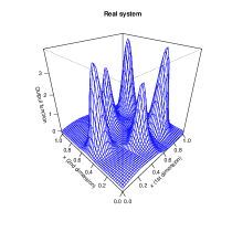
(a) Real system output function

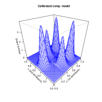
(b) Calibrated computer model

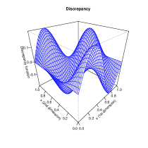
(c) Discrepancy

Figure 2: [Example 1] The output functions of the formulation $\zeta(x)=S(x,\theta_{x})+\delta(x)$

We generate a training data-set that consists of $n=50$ measurements from the real system and $m=120$ simulations from the computer model. For the observations, we generated randomly the input values, computed the corresponding system output values, and contaminated with random noise with variance $\sigma_{y}=0.02$. For the simulations, we randomly selected values for the input and model parameters through Latin hybercube sampling (LHS), computed corresponding the computer model output, and contaminated with noise with variance $\sigma_{\eta}=0.01$. For the IDBC-JPS, $\xi_{1}$, $\xi_{2}$, and $\xi_{3}$ share the same partition. For the IDBC-SPS, we consider that $\xi_{2}$ and $\xi_{3}$ share the same partition, while $\xi_{1}$ is associated with different partition. We use uniform priors on the calibration coefficients. The RJ-MCMC samplers consist of the grow & prune operations and the fixed dimensional operations as discussed in Section 3.2. Regarding the grow & prune operations, we used split & merge for $\xi_{1}$ and $\xi_{2}$ , and birth & death for $\xi_{3}$. The MCMC for each procedure ran for $2\times 10^{4}$ iterations, and the first $10^{4}$ ones were discarded as burn in.

The statistical methods under comparison are the standard Bayesian model calibration SBC, the IDBC-JPS with the joint partition scheme, and the IDBC-SPS with separate partition scheme. In Figures 3a, 3b, and 3c, we present histograms and trace plots of the generated MCMC samples of $\theta_{1,x}$ at input point $x_{0}=(0.5,0.4)$. We observe that SBC produces a rather flat posterior distribution, and hence it is unable to reduce uncertainty about $\theta_{1,x_{0}}$. The IDBC-JPS and IDBC-SPS have produced posteriors for $\theta_{1,x_{0}}$ whose main density is around the optimal value $\theta_{1,x_{0}}=0.5$. In particular, for posterior mode, mean and standard deviation estimates are $0.56$, $0.53$ and $0.29$ for SBC; $0.47$, $0.41$ and $0.16$ for IDBC-JPS; and $0.46$ and $0.14$ for IDBC-SPS. Although the three posterior modes and means seem to be close, the standard deviation showing the spread of the distribution is significantly smaller for IDBC-JPS and IDBC-SPS than what is for SBC. This indicates that unlike SBC, the proposed IDBC-JPS and IDBC-SPS methods have managed to reduce uncertainty about the unknown calibration parameter at $x_{0}$. We observe that the IDBC-SPS has produced a posterior density which is slightly more concentrated around the mode than that of IDBC-JPS, however this difference may be observed due to the variation of the MCMC approximation. In Figure 3d, we present the estimated sub-model selection probability of each sub-model at input point $x_{0}=(0.5,0.4)$. By construction the best sub-model is $\xi_{3}=2$. The selection probability estimate and standard error for $\xi_{3}=2$ at input point $x_{0}$ was $0.48$ ($0.004$) for SBC, $0.55$ ($0.004$) for IDBC-SPS, and $0.56$ ($0.004$) for IDBC-JPS. We observe that IDBC-JPS and IDBC-SPS have generated sub-model selection probabilities which suggest sub-model $\theta_{3,x_{0}}=2$ as the ‘best’ choice. On the other hand, SBC does not indicate which sub-model is preferable.

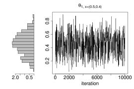
(a) IDBC-JPS

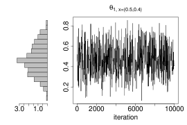
(b) IDBC-SPS

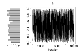
(c) SBC

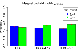
(d) Sub-model selection probability

Figure 3: [Example 5.1] Histograms of the posterior densities and trace plot of the MCMC samples for the generated optimal values for model parameters $\theta_{1}$ at input $x_{0}=(0.5,0.4)$. Sub-model selection probabilities coded in $\theta_{3}$ at input $x_{0}=(0.5,0.4)$, and the associated error bars. The procedures considered are SBC, IDBC-JPS, and IDBC-SPS.

In Figure 4, we present the RMSPE, as functions of the input, produced from the procedures SBC, IDBC-JPS, and IDBC-SPS. At each case, the root mean squared predictive error (RMSPE) was computed as the average of $10$ realizations of the corresponding procedure. We observe that the proposed IDBC-JPS and IDBC-SPS have produced smaller RMSPE than SBC, which indicates that the proposed methods produced better emulators than SBC.

We observe that IDBC-JPS and IDBC-SPS outperform SBC in the scenario of input dependent calibration parameters, however we cannot observe a significant difference between the performance of IDBC-JPS and IDBC-SPS.

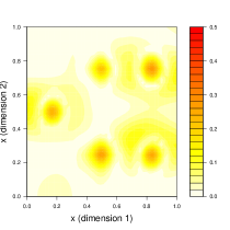
(a) SBC

(b) IDBC-JPS

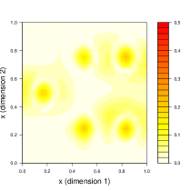
(c) IDBC-SPS

Figure 4: [Example 5.1] RMSPE as a function of input $x$ as produced by SBC, IDBC-JPS and IDBC-SPS. The RMSPE was computed by re-running each procedure $10$ times. The average RMSPE is (a): $0.071$ for SBC; (b): $0.046$ for IDBC-JPS; and (c): $0.044$ for IDBC-SPS.

5.2 A case study on a pollution computer model

We test the proposed method against the 2-D groundwater flow and solute transport model (Zhang et al., 2017). The study addresses the case that, under steady state water flow conditions, some amount of contaminant is released from a known source during the time interval $0[T]$ - $18[T]$. The transient saturated flow was considered in a $10[L]\times 16[L]$ domain uniformly discretized into $41\times 41$ grids. The upper and lower boundaries are no-flow, while the left and right boundaries are constant head boundaries with prescribed pressure heads of $16[L]$ and $10[L]$, respectively. It is assumed that there are $20$ measurement locations to collect data every $0.6[T]$ from $0[T]$ up to $18[T]$ time step, as shown in Figure 5d.

In the 2-D groundwater flow and solute transport model (Zhang et al., 2017), it is assumed that the uncertainty only stems from the connectivity field. The log conductivity field $Z$ was modeled as a spatially correlated Gaussian random field with a specific separable exponential correlation form (Zhang et al., 2017). Then the log conductivity field was parametrized through a Karhunen-Loève (KL) expansion, for dimension reduction reasons, as

$$Z(s|\xi_{i})\approx\bar{Z}(s)+\sum_{i=1}^{d}\xi_{i}\sqrt{\lambda_{i}}f_{i}(s),$$

where $s=(s_{1},s_{2})$ are spatial coordinates, $\bar{Z}(s)=0$ is the mean component, $\{\xi_{i}\}$ are independent standard Gaussian random variables, $\{\lambda_{i}\}$ and $\{f_{i}(s)\}$ are eigenvalues and eigenfunctions of the covariance function specifed. Here, we focus on calibrating $\xi_{1}$, and hence we consider it as an uncertain calibration parameter. The inputs are the spatial coordinates $s$ and the time $\chi$, hence $x=(s_{1},s_{2},\chi)$. The quantity of interest, according to which the model parameters are calibrated, is the concentration of the contaminant source which is an important index in pollution control; and hence it is the output $y(x)$. Calibrating $\xi$ is important because it determines the conductivity field which can be used to locate the contamination source.

For the purpose of the example, we artificially introduce an input dependence to the optimal model parameter values. Precisely, if $C_{s}(x,\xi)$ is the concentration with respect to inputs and parameters as described in (Zhang et al., 2017), then the computer model output is assumed to be $S(x,t):=C_{s}(x|\xi=(\xi_{0}+\theta_{x})-t)$, where

$$\theta_{x}=\begin{cases}0&,\,x_{1}<10,\\ 2&,\,x_{1}>10,\,x_{2}<4.5\\ -2&,\,x_{1}>10,\,x_{2}>4.5\end{cases}.$$ (22)

This artificially introduces input dependence on the optimal model parameter values, and obviously $\zeta(x)=S(x,t=\theta_{x})$. Note that in (22), the calibration parameters are invariant to the time step.

We consider, that there is available a sample of $500$ points; precisely $50$ model evaluations at $10$ time steps. The experimental training data were generated such that $\xi_{0}=0.5$ from the original model of Zhang et al. (2017). We wish to recover an estimate for (22), as well as to produce an emulator for the concentration. We compare the proposed procedure IDBC-JPS with SBC. In the statistical model (4), the discrepancy term is set to zero as assumed by the example. We use the prior model in (6), and we assign uniform priors on the calibration coefficients in the range $[-10,10]$.

The RJ-MCMC samplers consist of the grow & prune operations and the fixed dimensional operations as discussed in Section 3.2. In particular, we include two distinct RJ updates one is the grow & prune operation with split & merge, and the other is the grow & prune operation with birth & death. Regarding the split & merge, we used $g(\vartheta)=\textup{logit}(0.05(\vartheta-10))$ which is a re-scaled version of (Table 1; 4th line); and the auxiliary proposal was generated from $u\sim\text{sBe(2,2,2)}$. The birth & death operation is used in the default form (Section 3.2). The MCMC samplers for each procedure ran for $2\times 10^{4}$ iterations, and the first $10^{4}$ ones were discarded as burn in. The split & merge produced more acceptable RJ transitions than the birth & death ones. The estimated expected acceptance probability was $8\%$ for split & merge, and $5\%$ for birth & death. Possibly birth & death produced higher a rejection rate than the split & merge because of the vague prior of the calibration coefficient which causes the former to propose randomly large changes.

In Figures 5, we present histograms and trace plots for calibration parameters produced by the proposed IDBC method at three different locations (input points), as well as those produced by the SBC. We observe that, at the three input points, the posterior densities of the calibration parameters produced by IDBC are concentrated above areas around the ideal values. We observe that the SBC concentrates the posterior density around value $3$, which is far from the ideal values. Therefore, we observe that, unlike SBC, IDBC manages to reduce uncertainty about the optimal values of the calibration parameters.

(a) IDBC at $x=(7,5,*)$

(b) IDBC at $x=(13,6.5,*)$

(c) IDBC at $x=(13,3,*)$

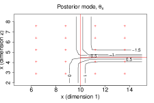
(d) IDBC (MAP estimate)

(e) SBC

Figure 5: [Example 5.2] Estimates of the optimal values of the model parameter at input points $(13,3,*)$, $(13,6.5,*)$, $(7,5,*)$. The $*$ indicates that the estimate refers to any time step. The methods presented are the IDBC-JPS, and SBC. The red lines indicate the boundaries of the real partition. The red crosses denote the $20$ measurement locations assumed. The estimated optimal values are $\theta_{x=(7,5,*)}^{(\text{IDBC})}=-0.04$, $\theta_{x=(13,6.5,*)}^{(\text{IDBC})}=-1.58$, $\theta_{x=(13,3,*)}^{(\text{IDBC})}=1.69$, and $\theta^{(\text{SBC})}=3.1$.

In Figure 6, we present the RMSPE produced by the proposed IDBC and the standard SBC, as function of the time step, at three different locations. We observe that RMSPE produced by IDBC is smaller than that produced by SBC , and hence IDBC has produced more accurate predictions than the standard SBC.

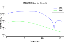
(a) $s_{1}=7$, $s_{2}=5$

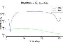
(b) $s_{1}=13$, $s_{2}=6,5$

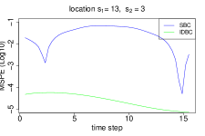
(c) $s_{1}=13$, $s_{2}=3$

Figure 6: RMSPE (in Log10 scale) of the contamination produced by IDBC and SBC, at three different locations, as function of time. The average RMSPE is (in Log10 scale) (a): $-3.19$ for IDBC,$-1.83$ for SBC; (b): $-3.84$ for IDBC, $-1.76$ for SBC; (c): $-3.84$ for IDBC, $-1.41$ for SBC.

5.3 Application to large-scale climate modeling

We consider the Advanced Research Weather Research and Forecasting Version 3.2.1 (WRF Version 3.2.1) climate model (Skamarock et al., 2008) constrained in the geographical domain $25^{\circ}\text{--}44^{\circ}\text{N}$ and $112^{\circ}\text{--}90^{\circ}\text{W}$ over the Southern Great Plains (SGP) region, and we concentrate on the average monthly precipitation response. Here, we briefly discuss the application, however more details can be found in (Yang et al., 2012; Karagiannis and Lin, 2017).

WRF is employed with the Kain-Fritsch convective parametrisation scheme (KF CPS) (Kain, 2004) as in (Yang et al., 2012). The $5$ most critical parameters (Yang et al., 2012) of the KF scheme are: the coefficient related to downdraft mass flux rate $P_{\text{d}}$ that takes values in range $[-1,1]$; the coefficient related to entrainment mass flux rate $P_{\text{e}}$ that takes values in range $[-1,1]$; the maximum turbulent kinetic energy in sub-cloud layer ($m^{2}s^{-2}$) $P_{\text{t}}$ that takes values in range $[3,12]$; the starting height of downdraft above updraft source layer (hPa) $P_{\text{h}}$ that takes values in range $[50,350]$; and the average consumption time of convective available potential energy $P_{\text{c}}$ that takes values in range $[900,7200]$. The ranges of the KF CPS parameters are quite wide and hence cause higher uncertainties in climate simulations due to the non linear interactions and compensating errors of the parameters (Gilmore et al., 2004; Murphy et al., 2007; Yang et al., 2012). We consider two different radiation schemes, the Rapid Radiative Transfer Model (RRTMG) for General Circulation Models (Mlawer et al., 1997), and the Community Atmosphere Model 3.0 (CAM) (Collins et al., 2004). Which radiation scheme is suitable to use in the computer model may depend on the input coordinates Yan et al. (2014).

The available sub-models are the two radiation schemes RRTMG and CAM. The sub-models are coded as $0$-1 orthogonal contrasts, and considered as levels of a categorical calibration parameter. The $5$ KF CPS parameters are considered as standard continuous calibration parameters. The output is the monthly average precipitation (in $\log\,mm$ ) and the input are the coordinates in SGP region.

Experimental data consist of $404$ measurements from stations in the geographical domain $25^{\circ}\text{--}44^{\circ}\text{N}$ and $112^{\circ}\text{--}90^{\circ}\text{W}$ over the SGP region, and represent monthly average precipitation (in $mm$) in June $2007$. The data-set is available from the U.S. Historical Climatological Network repository (Karl et al., 1990). The simulation data consist of a simple random sample of size $1000$ from the original data-set generated by Yan et al. (2014). We analyze the problem by using the proposed IDBC. We use the GP statistical model described in Section 2.2 with mean functions and tapering covariance functions used in (Karagiannis and Lin, 2017). The MCMC sampler consists of the grown & prune operations, and the fixed dimensional updates discussed in the Section 3.2. In particular, regarding the grow & prune operations, we used the birth & death for the sub-models, and split & merge for the KF CPS parameters. The MCMC samplers ran for $10000$ where the first half iterations where discarded as burn-in.

In our analysis, the uncertainty of the model to convective parameterization, as well as that of the choice of the ‘best’ radiation scheme, is quantified with respect to the geographical coordinates. In Figures 7a-7e, we present the estimates of the calibration parameters with respect to the input space, as computed by the MAP estimator (posterior mode). Regarding the KF CPS parameters, we observe that they slightly change in value throughout the SGP region. In Figure 7f, we observe that the CAM sub-model can be considered as a ‘best’ choice to run at regions like Nebraska and Iowa, while the RRTMG is ‘better’ to be used in the WRF model at regions like Texas and Arizona. The results produced by the proposed method are consistent to the results in (Karagiannis and Lin, 2017) and the discussion in presented in a different context.

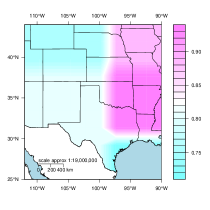
(a) $P_{\text{d}}$

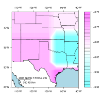
(b) $P_{\text{e}}$

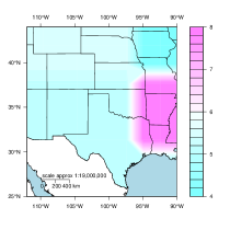
(c) $P_{\text{t}}$

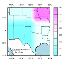
(d) $P_{\text{h}}$

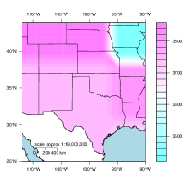
(e) $P_{\text{c}}$

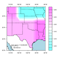
(f) Sub-model selection probability of RRTM

Figure 7: [Example 3] MAP estimates of the calibration parameters produced from IDBC. Figures (a)-(e): the MAP estimates of the optimal values for KF CPS parameters. Figure (f): the probability of RRTMG to be the ‘best’ radiation scheme.

6 Discussion

We proposed a new fully Bayesian method for the calibration of computer models with uncertain parameters whose optimal values may depend on the inputs. The proposed method provides optimal model parameter values as functions of the input, as well as the associated posterior distribution that characterizes their uncertainty. The proposed method is especially useful in cases that running the computer model requires the choice of a sub-model from a set of available ones, but this ‘best’ choice may be different at different input regions. The method produces a sub-model selection probability that indicates which sub-model is the ‘best’ choice at a given input. We provided two variations of the method: the IDBC-JPS assuming that all the dimensions of the calibration parameter share the same partition of the input domain, and IDBC-SPS (in Appendix A) allowing them to be associated to different partitions. In order to address the challenging computations, we proposed reversible jump operations suitable to the proposed method.

The performance of the IDBC was assessed against benchmark examples, and compared to the standard Bayesian calibration method. We observed that in scenarios where the optimal calibration parameter values or the choice of the ‘best’ sub-model depends on the model inputs, the proposed method tends to produce more accurate results. We observed that, the proposed method, produces more accurate emulators (predictive models) that the standard Bayesian model calibration. In our comparable example, IDBC-JPS and IDBC-SPS presented similar performance; hence IDBC-SPS should be mainly used when there is need to obtain simpler partitions for interpretation reasons. The proposed method was utilized to analyze a real world problem that involves the calibration of the WRF computer model with two competing sub-models.

Up to our knowledge, the proposed method is a first of its kind, where the calibration parameters are modeled as functions of input sub-regions, and hence it creates new directions for research. At this stage, the proposed method has been developed to calibrate computer models with univariate outputs only. Hence, IDBC can be extended to address problems with computer models producing multivariate outputs with dependent dimensions as in (Bilionis and Zabaras, 2012). The computational cost of the current IDBC implementation can be very expensive in cases with many input dimensions (e.g., $50$). To address such cases, the method can possibly be coupled with ideas from (Linkletter et al., 2006), and (Higdon et al., 2008). In another extension, sequential Monte Carlo ideas can be used as in (Taddy et al., 2011) to alleviate the cost of Bayesian computations. These topics are ongoing projects and their results will be presented in future publications.

Appendix

Appendix A Separate partition scheme

The binary tree mechanism is expected to split the input space when at least one dimension of the calibration parameter significantly changes in value. In scenarios where several dimensions of the calibration parameter present significantly different values around different areas of the input space, the joint partition scheme may lead to a complex partition with a large number of sub-regions which is difficult to interpret.

IDBC can use a separate partition scheme (IDBC-SPS). Let $\boldsymbol{\theta_{x}}:=(\theta_{x,1},...,\theta_{x,C})$ denote the separation of the whole vector of calibration parameters in groups $\theta_{x,c}$, where $\theta_{x,c}$ is modeled as in (5). The dimensions of the calibration parameter within a group are assumed to share the same partition, but those between different groups may have different partitions. Let $(\boldsymbol{\vartheta},\boldsymbol{\mathcal{T}}):=(\vartheta_{c},\mathcal{T}_{c};c=1,...,C)$ denote the hyper-parameters of $\boldsymbol{\theta_{x}}$, then $(\boldsymbol{\vartheta},\boldsymbol{\mathcal{T}})$ follows a priori distribution

$$\pi(\boldsymbol{\vartheta},\boldsymbol{\mathcal{T}})=\prod_{c=1}^{C}\pi(\vartheta_{c},\mathcal{T}_{c}),$$

where $\pi(\vartheta_{c},\mathcal{T}_{c})$ is defined as in Section 3.1 for $c=1,...,C$. The derivation of the posterior distribution is straightforward as in Section 3.1; $\pi(\boldsymbol{\vartheta},\boldsymbol{\mathcal{T}},\beta,\varphi|z)\propto f(z|\boldsymbol{\theta_{x}},\beta,\varphi)\pi(\boldsymbol{\vartheta},\boldsymbol{\mathcal{T}})\pi(\varphi)\pi(\beta).$ In the MCMC sampler, the block $[\boldsymbol{\vartheta},\boldsymbol{\mathcal{T}}|z,...]$ is updated by a random scan of $C$ grow & prune operations each of them targeting the conditionals $\pi(\vartheta_{c},\mathcal{T}_{c}|z,\vartheta_{-c},\mathcal{T}_{-c},\varphi)$ for $c=1,...,C$. These operations were discussed in Section 3.1.

The separate partition scheme aims at producing several simpler partitions which are easier to interpret. If calibration parameters are properly separated, each binary tree partition will be responsible to divide the input domain at sub-regions according to the corresponding calibration parameter changes. Hence, the main advantage of IDBC-SPS compared to IDBC-JPS is that, instead of producing a single complex partition with a large number of sub-regions, IDBC-SPS is expected to produce simpler partitions with less sub-regions that will be easier to interpret.

How the calibration parameters are separated into groups is problem dependent. One can use prior knowledge from the domain scientist regarding the governing equations of the computer model. A sensible rule is that, calibration parameters sharing the same partition should be expected to present similar behavior with respect to the input, while those admitting separate partitions must tend present different ones.

References

- Andrieu and Thoms (2008) Andrieu, C. and J. Thoms (2008). A tutorial on adaptive MCMC. Statistics and Computing 18(4), 343–373.
- Bélisle et al. (1993) Bélisle, C. J., H. E. Romeijn, and R. L. Smith (1993). Hit-and-run algorithms for generating multivariate distributions. Mathematics of Operations Research 18(2), 255–266.
- Bhat et al. (2014) Bhat, K. S., D. S. Mebane, C. B. Storlie, and P. Mahapatra (2014). Upscaling uncertainty with dynamic discrepancy for a multi-scale carbon capture system. arXiv preprint arXiv:1411.2578.
- Bilionis and Zabaras (2012) Bilionis, I. and N. Zabaras (2012). Multi-output local gaussian process regression: Applications to uncertainty quantification. Journal of Computational Physics 231(17), 5718 – 5746.
- Brynjarsdóttir and O’Hagan (2014) Brynjarsdóttir, J. and A. O’Hagan (2014). Learning about physical parameters: The importance of model discrepancy. Inverse Problems 30(11), 114007.
- Chipman et al. (1998) Chipman, H. A., E. I. George, and R. E. McCulloch (1998). Bayesian cart model search. Journal of the American Statistical Association 93(443), 935–948.
- Collins et al. (2004) Collins, W. D., P. J. Rasch, B. A. Boville, J. J. Hack, J. R. McCaa, D. L. Williamson, J. T. Kiehl, B. Briegleb, C. Bitz, S. Lin, et al. (2004). Description of the ncar community atmosphere model (cam 3.0).
- Cressie (1993) Cressie, N. (1993). Statistics for Spatial Data: Wiley Series in Probability and Statistics. Wiley: New York, NY, USA.
- Gilmore et al. (2004) Gilmore, M. S., J. M. Straka, and E. N. Rasmussen (2004). Precipitation uncertainty due to variations in precipitation particle parameters within a simple microphysics scheme. Monthly weather review 132(11), 2610–2627.
- Gramacy and Lee (2012) Gramacy, R. B. and H. K. Lee (2012). Cases for the nugget in modeling computer experiments. Statistics and Computing 22(3), 713–722.
- Green (1995) Green, P. (1995). Reversible jump Markov chain Monte Carlo computation and Bayesian model determination. Biometrika 82(4), 711–732.
- Higdon et al. (2013) Higdon, D., J. Gattiker, E. Lawrence, C. Jackson, M. Tobis, M. Pratola, S. Habib, K. Heitmann, and S. Price (2013). Computer model calibration using the ensemble kalman filter. Technometrics 55(4), 488–500.
- Higdon et al. (2008) Higdon, D., J. Gattiker, B. Williams, and M. Rightley (2008). Computer model calibration using high-dimensional output. Journal of the American Statistical Association 103(482).
- Kain (2004) Kain, J. S. (2004). The kain-fritsch convective parameterization: an update. Journal of Applied Meteorology 43(1), 170–181.
- Karagiannis and Andrieu (2013) Karagiannis, G. and C. Andrieu (2013). Annealed importance sampling reversible jump MCMC algorithms. Journal of Computational and Graphical Statistics 22(3), 623–648.
- Karagiannis and Lin (2017) Karagiannis, G. and G. Lin (2017). On the bayesian calibration of computer model mixtures through experimental data, and the design of predictive models. Journal of Computational Physics 342, 139–160.
- Karl et al. (1990) Karl, T., C. Williams, F. Quinlan, and T. Boden (1990). United states historical climatology network (hcn) serial temperature and precipitation data, environmental science division, publication no. 3404. Technical report, Carbon Dioxide Information and Analysis Center, Oak Ridge National Laboratory, Oak Ridge, TN, 389 pp.