Abstract

We investigate in this paper the Landau-Lifshitz energy distribution in the framework of $f(T)$ theory view as a modified version of Teleparallel theory. From some important Teleparallel theory results on the localization of energy, our investigations generalize the Landau-Lifshitz prescription from the computation of the energy-momentum complex to the framework of $f(T)$ gravity as it is done in the modified versions of General Relativity. We compute the energy density in the first step for three plane symmetric metrics in vacuum. We find for the second metric that the energy density vanishes independently of $f(T)$ models. These metrics provide results in perfect agreement with those mentioned in literature. In the second step the calculations are performed for the Cosmic String Spacetime metric. It results that the energy distribution depends on the mass $M$ of cosmic string and it is strongly affected by the parameter of the considered $f(T)$ quadratic model.

1 Introduction

To express the energy-momentum as a unique tensor quantity or in other formulation, the problem of the localization of energy in General Relativity, has been since an open problem in this branch of theoretical physic. Indeed, the localization of energy-momentum is one of the oldest and thorny problems [1] in General Relativity (GR) which is still without any acceptable answer in general. In order to solve the problem, several attempts have been made, starting by Einstein who was the first to introduce locally conserved energy-momentum pseudo tensors known as energy-momentum complex[2]. Being a natural field, it is expected that gravity should have its own local energy-momentum density. Misner, Thorne and Wheeler[1] argued that the energy is localizable only for spherical systems. This viewpoint has been contradicted by Cooperstock and Sarracino [3]. They stipulated that if energy can be localized in spherical systems, it can also be localized for all systems. Bondi [4] agreed with them and argued that one can not admit in GR a non-localizable form of energy whose location can in principle be found. Through several very interesting works, different definitions for the energy and momentum distributions have been introduced by others physicists in RG and others equivalent theories, namely MØller [5], Tolman[6], Landau-Lifshitz [7], Papapetrou [8], Bergmann-Thomson [9], Weinberg[10], Qadir-Sharif[11], Mikhail[12], Vargas[13]. All these prescriptions, except MØller, are restricted to perform calculations in Cartesian coordinates only. Recently Virbhadra [14] remarked that the concept of energy-momentum complexes are very useful in investigating the Seifert conjecture for naked singularities and the hoop conjecture of Thorne. By considering this fundamental result, Chang and his collaborators [15] proved that every energy-momentum complex can be associated with a particular Hamiltonian boundary term. Thus the energy-momentum complexes may also be considered as quasi-local. Landau-Lifshitz [7] introduced the energy-momentum complex by using the geodesic coordinate system at some particular point of space. Why studying the gravitational energy density? The gravitational energy density plays a remarkable role in the description of the total energy of the universe. Firstly, it is mentioned in literature that at the time of the creation of our universe which results from quantum fluctuation of the vacuum, any conservation law of physics need not to have been violated [16]. Indeed, Tryon [16] in same idea as Albrow [17] suggested that our universe must have a zero net value for all conserved quantities. They supported their point of view by using a Newtonian order of magnitude estimate and obtained that the net energy of our universe may be indeed zero. By using Killing vectors, Cooperstock and Israelites [18] have initiated a real and interesting work on the energy-momentum distributions of the open and closed universes They found zero as the value of energy for any homogeneous isotropic universe described by a Friedmann-Robertson-Walker metric in the context of General Relativity. This result has been confirmed by many other authors through different works on metrics describing these kinds of universes [13, 19]. Secondly, in attempt to answer the previous question, some authors like [20] and it collaborators, argued that during inflation the vacuum energy driving the accelerated expansion of the universe, and which was responsible for the creation of radiation and matter in the universe, is drawn from the energy of the gravitational field.

Recently, the problem of energy-momentum localization was also considered in modified theories of General Relativity, the so called $f(R)$ theory [21, 22] as in Teleparallel gravity [12, 13, 23] and its modified version namely $f(T)$ theory[24]. Teleparallel gravity is an alternative description of gravitation which corresponds to a gauge theory for the translation group [25]. There are already no bad number of papers, on the energy-momentum localization in this theory. The authors found that the problem of energy-momentum localization can also be discussed in this alternative theory, their results are in agreement with those found in GR. For example, in [13], Vargas established the Einstein and Landau-Lifshitz energy-momentum complex in the framework of Teleparallel gravity and found zero for the total energy in Friedmann-Robertson-Walker space-times. Among other interesting works, we can note that of Of Mustafa [26]. The author used the MØller, Einstein, Bergmann-Thomson, and Landau-Lifshitz prescriptions in both GR and Teleparallel gravity to evaluate the energy distribution for the generalized Bianchi-type I metric. For the first time in literature, Ulhoa and Spaniol [24] presented and analyzed an expression for the gravitational energy-momentum vector in the context of $f(T)$ theories. They also obtained a vanishing gravitational energy for a particular choice of the tetrad.
In this paper, we propose to investigate the same aspect of Landau-Lifshitz in the context of the modified Teleparallel $f(T)$ gravity. Our main goal in this work is to extract the Landau-Lifshitz energy-momentum complex valid for $f(T)$ theory. Then, we aim to evaluate the corresponding energy density for some particular metrics. Our investigation was motivated by the fact that the Landau-Lifshitz energy-momentum complex in particular has been recently at the center of very interesting discussions in GR and in the framework of $f(R)$ theory. The Laudau-Lifshitz energy distribution has been calculated for two metrics which describe non-asymptotically flat black hole solutions in dilaton-Maxwell gravity [27]. This investigation shows that the obtained energies depended on the mass, the charge of the black hole and the parameter of these metrics. In addition, the authors in [21] generalized for the first time the Landau-Lifshitz prescription from the computation of the energy-momentum complex to the framework of $f(R)$ gravity with constant scalar curvature as necessary condition. Some time after Sharif and Shamir [22] used this energy-momentum complex to evaluate in the framework of $f(R)$, the energy density of three plane symmetric metrics and for cosmic string spacetime.
The paper is organized as follows. In section Sec.II, we review some fundamental results on the Landau-Lifshitz energy-momentum complex in the Teleparallel theory. This have allowed us to establish at the end of the section, the generalized Landau-Lifshitz energy-momentum complex valid for the so-called $f(T)$ gravity. In section Sec.III, we compute the obtained energy density for plane symmetric metrics. The section Sec.III is devoted to energy distribution of cosmic string spacetime metric. The conclusion comes in the last section.

2 Teleparallel and $f(T)$ versions of Landau-Lifshitz Energy-Momentum Complexe ($EMC$)

Through the revision of the fundamental results on the Landau-Lifshitz Energy-Momentum Complex in the Teleparallel theory, we will establish the generalized Landau-Lifshitz energy-momentum complex valid for the $f(T)$ theory. Before giving the Teleparall version of the Landau-Lifshitz energy-momentum complex, we briefly outline the main points of the Teleparall theory. In general, when formulating theories of gravity, the metric tensor is of paramount importance. It contains the information needed to locally measure distances and thus to make theoretical predictions about experimental findings. Furthermore, the structure of the spacetime can be described by an alternative dynamical variable, the well known non-trivial tetrad $h^{a}_{\;\;\mu}$ which is a set of four vectors defining a local frame at every point. The tetrads represent the basic entity of the theory of Teleparallel gravity. From their reconstruction arises the Teleparall theory as gravitational theory naturally based on the gauge approach of the group of translations. The tretrads are defined from the gauge covariant derivative for a scalar field as $h^{a}_{\;\;\mu}=\partial_{\mu}x^{a}+A^{a}_{\;\;\mu}$ with $A^{a}_{\;\;\mu}$ the translational gauge potential and $x^{a}$ the tangent-space coordinates [28]. The tretrad $h^{a}_{\;\;\mu}$ and its inverse $h_{a}^{\;\;\mu}$ satisfy the following relations:

$$h^{a}_{\;\;\mu}h_{a}^{\;\;\nu}=\delta^{\nu}_{\mu}\quad\quad h^{a}_{\;\;\mu}h_{b}^{\;\;\mu}=\delta^{a}_{b}.$$ (1)

An another important notion resulting from the establishing of this theory is the condition of absolute parallelism [29] which leads to the Weitzenböck connection seen as the fundamental connection of the theory. It is given by

$$\Gamma_{\mu\nu}^{\lambda}=h_{a}^{\;\;\lambda}\partial_{\nu}h^{a}_{\;\;\mu}=-h^{a}_{\;\;\mu}\partial_{\nu}h_{a}^{\;\;\lambda}.$$ (2)

. We emphasize here that the Latin alphabet $(a,b,c,...=0,1,2,3)$ is used to denote the tangent space indices and the Greek alphabet $(\mu,\nu,\rho,...=0,1,2,3)$ to denote the spacetime indices. The metric and the tetrad are related by

$$g_{\mu\nu}=\eta_{ab}h^{a}_{\;\;\mu}h^{b}_{\;\;\nu},$$ (3)

where $\eta_{ab}=\text{diag}(+1,-1,-1,-1)$ is the Minkowski metric of the tangent space. In Teleparallel gravity and due to the no curvature Weitzenböck connection, the effects of gravitation are described by the torsion tensor, while curvature tensor does not appear. Consequently, the non-vanishing and naturally antisymmetric torsion tensor is expressed via its components by

$$T_{\;\;\;\mu\nu}^{\lambda}=\Gamma_{\;\;\;\nu\mu}^{\lambda}-\Gamma_{\;\;\;\mu\nu}^{\lambda}=h_{a}^{\;\;\lambda}(\partial_{\mu}h^{a}_{\;\;\nu}-\partial_{\nu}h^{a}_{\;\;\mu})\neq 0.$$ (4)

Another important tensor emerging from the use of the Weitzenböck connection is the contortion tensor $K_{\;\;\;\mu\nu}^{\;\,\lambda}$ which shows the difference between the Weitzenböck connection and the Levi-Civita connection [30] according to

$$K_{\;\;\;\mu\nu}^{\lambda}:=\Gamma_{\;\;\;\mu\nu}^{\lambda}-\tilde{\Gamma}_{\;\;\;\mu\nu}^{\lambda}=\frac{1}{2}\Big{(}T_{\nu}{}^{\lambda}{}_{\mu}+T_{\mu}{}^{\lambda}{}_{\nu}-T^{\lambda}{}_{\mu\nu}\Big{)},$$ (5)

where $\tilde{\Gamma}_{\;\;\;\mu\nu}^{\;\,\lambda}$ are the Christoffel symbols or the coefficient of Levi-Civita connection. The action of Teleparallel gravity in the presence of matter is given by

$$S=\frac{1}{\kappa^{2}}\int d^{4}xhT+\int d^{4}xh\mathcal{L}_{M},$$ (6)

where $h=|\text{det}(h^{a}{}_{\mu})|$ is equivalent to $\sqrt{-g}$ in General Relativity, $\kappa^{2}=\frac{16\pi G}{c^{4}}$, $\mathcal{L}_{M}$ is the Lagrangian of the matter field and $T$ the scalar torsion defined by

$$T:=S_{\beta}{}^{\mu\nu}T{}^{\beta}{}_{\mu\nu},$$ (7)

with $S_{\beta}{}^{\mu\nu}$, specifically defined by [29]

$$S_{\beta}{}^{\mu\nu}=\frac{1}{2}\Big{(}K{}^{\mu\nu}{}_{\beta}+\delta^{\mu}_{\beta}T{}^{\alpha\nu}{}_{\alpha}-\delta^{\nu}_{\beta}T{}^{\alpha\mu}{}_{\alpha}\Big{)}.$$ (8)

The variation of (6) with respect to $h^{a}{}_{\mu}$ leads to the Teleparallel field equations with $c^{4}=1$,

$$\partial_{\nu}(hS_{\beta}{}^{\mu\nu})-4\pi G(ht^{\mu}{}_{\beta})=4\pi GhT^{\mu}{}_{\beta},$$ (9)

where $T^{\mu}{}_{\beta}=-h^{-1}h^{a}_{\;\;\beta}\Bigg{[}\frac{\partial\mathcal{L}_{m}}{\partial h^{a}_{\;\;\mu}}-\partial_{\alpha}\frac{\partial\mathcal{L}_{m}}{\partial(\partial_{\alpha}h^{a}_{\;\;\mu})}\Bigg{]}$ is the energy-momentum tensor of the matter fields and

$$t^{\mu}{}_{\beta}=\frac{1}{4\pi G}h\Gamma_{\beta\lambda}^{\nu}S_{\nu}{}^{\mu\sigma}-\delta^{\mu}_{\lambda}\mathcal{L}_{G}$$ (10)

is the energy-momentum pseudotensor of the gravitational field [31]. Furthermore, the equation (9) can be rewritten in the following relation

$$h(t^{\mu}{}_{\beta}+T^{\mu}{}_{\beta})=\frac{1}{4\pi G}\partial_{\nu}(hS_{\beta}{}^{\mu\nu}).$$ (11)

From this relation and due to the antisymmetry of the tensor $S_{\beta}{}^{\mu\nu}$ in its last indices, one can extract the conservation law in the following relation

$$\partial_{\mu}[h(t^{\mu}{}_{\beta}+T^{\mu}{}_{\beta})]=0.$$ (12)

According to the equivalence between the Teleparallel equation and the Einstein’s equations [28], the Teleparallel tensor $U_{\beta}{}^{\mu\nu}=hS_{\beta}{}^{\mu\nu}$ stays for the Freud’s superpotential [13],[32], [26] and [33]. Consequently, $t^{\mu}{}_{\beta}$ is nothing but the Teleparallel version of Einstein’s gravitational energy-momentum pseudotensor. In addition this Teleparallel version of Freud’s superpotential is directly related to the geometrical density Lagrangian $\mathcal{L}_{G}$ via the fundamental relation [13]

$$U_{\beta}{}^{\mu\nu}=4\pi Gh^{a}_{\;\;\beta}\frac{\partial\mathcal{L}_{G}}{\partial(\partial_{\nu}h^{a}_{\;\;\mu})}$$ (13)

The Landau-Lifshitz’s energy-momentum complex in Teleparallel gravity given as follow [13]

$$hL^{\mu\nu}=\frac{1}{4\pi G}\partial_{\sigma}(hg^{\mu\lambda}U_{\beta}{}^{\nu\sigma}).$$ (14)

According to (12), the Landau-Lifshitz’s energy-momentum complex $L^{\mu\nu}$ satisfies the local conservation laws $\frac{\partial L^{\mu\nu}}{\partial x^{\nu}}=0$ .

The energy and momentum distributions of Landau-Lifshitz prescription in the Teleparallel gravity are summarized in the following equation [13]:

$$P_{\mu}=\int_{\sum}hL^{0}{}_{\mu}dxdydz,$$ (15)

where $P_{\mu}$ for $\mu=1,2,3$ gives the momentum components and $P_{0}$ stays for the energy. The integration hypersurface $\sum$ is described by $x^{0}=t=$constant. In the following paragraph, we are searching for the expression the of Landau-Lifshitz’s energy-momentum complex in the framework a Teleparallel modified version namely $f(T)$ theory.

The action of the modified versions of TEGR (Teleparallel equivalent of General Relativity [34] is obtained by substituting the scalar torsion of the action (6) by an arbitrary function of scalar torsion obtaining modified theory $f(T)$. This approach is similar in spirit to the generalization of Ricci scalar curvature of Einstein-Hilbert action by a function of this scalar leading to the well known $F(R)$ theory. Indeed, the action of $f(T)$ theory can be defined as

$$S=\frac{1}{\kappa^{2}}\int d^{4}xhf(T)+\int d^{4}xh\mathcal{L}_{M}.$$ (16)

The variation of this action with respect to tetrad $h_{a}{}^{\mu}$ gives ( [24], [35] and [36])

$$\frac{1}{h}\partial_{\mu}(hS_{a}{}^{\mu\nu})f_{T}(T)-h_{a}{}^{\lambda}T^{\rho}{}_{\mu\lambda}S_{\rho}{}^{\mu\nu}f_{T}(T)+S_{a}{}^{\mu\nu}\partial_{\mu}(T)f_{TT}(T)+\frac{1}{4h}h_{A}{}^{\nu}f(T)=\frac{1}{4\kappa^{2}}T^{\nu}_{a},$$ (17)

with $f_{T}(T)=df(T)/dT$, $f_{TT}(T)=d^{2}f(T)/dT^{2}$. The field equations can be recast in the following form [24])

$$\partial_{\sigma}\Big{[}hS^{a\tau\sigma}f_{T}(T)\Big{]}=\frac{1}{4\kappa^{2}}h^{a}{}_{\lambda}\Big{(}t^{\tau\lambda}+T^{\tau\lambda}\Big{)},$$ (18)

where

$$t^{\tau\lambda}=\frac{1}{\kappa^{2}}\Big{[}4f_{T}(T)g^{\lambda\beta}S_{\mu}{}^{\nu\tau}T^{\mu}{}_{\nu\beta}-g^{\tau\lambda}f(T)\Big{]}.$$ (19)

Due to the skew-symmetry of $S_{\mu}{}^{\nu\tau}$ in the two up indices, it follows that

$$\partial_{\tau}\partial_{\sigma}[hS^{a\tau\sigma}]\equiv 0,$$ (20)

and one obtains

$$\partial_{\tau}(ht^{a\tau}+hT^{a\tau})=0.$$ (21)

We note here that the above expression works as a conservation law for the sum of the energy-momentum tensor of matter fields and the quantity $t^{\tau\lambda}$ . Thus $t^{\tau\lambda}$ is interpreted as the energy-momentum tensor of the gravitational field in the context of $f(T)$ theories [24], being more general than (and slightly different from) the usual quantity in Teleparallel presented in (10). However, making using the Laudau-Lifshitz prescription [7] and its applications in the context of Teleparallel gravity as it was done in [13], one can rewrite the equation (18) in the following form

$$\frac{1}{4\pi G}\partial_{\nu}[g^{\tau\sigma}h\tilde{U}_{\sigma}{}^{\lambda\nu}]=h^{2}(t^{\tau\lambda}+T^{\tau\lambda}),$$ (22)

where

$$\tilde{U}_{\sigma}{}^{\lambda\nu}=4\pi Gh^{a}_{\;\;\sigma}\frac{\partial\tilde{\mathcal{L}}_{G}}{\partial(\partial_{\lambda}h^{a}_{\;\;\nu})},$$ (23)

with $\tilde{\mathcal{L}}_{G}=\frac{1}{\kappa^{2}}hf(T)$. Consequently, the tensor $\tilde{U}_{\sigma}{}^{\lambda\nu}$ can be interpreted as the Freud’s super-potential tensor in the contexte of $f(T)$ theory and it generalizes its Teleparallel version found by [13] (i.e for $f(T)=T$ we get $U_{\sigma}{}^{\lambda\nu}$ in (13)). In addition, Following the same approach as [13], we deduct simply the $f(T)$ version of the Laudau-Lifshitz energy-momentum complex as

$$h\tilde{L}^{\tau\lambda}=\frac{1}{4\pi G}\partial_{\nu}[g^{\tau\sigma}h\tilde{U}_{\sigma}{}^{\lambda\nu}],$$ (24)

or in equivalent form as it is established in General Relativity [26, 33] and its modified versions [21, 22] as

$$h\tilde{L}^{\tau\lambda}=h^{2}(t^{\tau\lambda}+T^{\tau\lambda}).$$ (25)

Here $h^{2}$ can be identified to $-g$ in General Relativity. As conclusion, $T^{\tau\lambda}$ is usually the energy-momentum tensor of the matter and all non-gravitational fields, and $t^{\tau\lambda}$ in (19) is the $f(T)$ version of Landau-Lifshitz energy-momentum pseudo tensor. So, the locally conserved quantity $h\tilde{L}^{\tau\lambda}$ contains contributions from the matter, non-gravitational fields and gravitational fields.

In order to facilitate the calculation, we rewrite the generalized Landau-Lifshitz energy-momentum complex $h\tilde{L}^{\tau\lambda}$ of (24) in term of Teleparallel quantities via the following relation,

$$h\tilde{L}^{\tau\lambda}=f_{T}(T)hL^{\tau\lambda}+\frac{1}{4\pi G}hg^{\tau\sigma}U_{\sigma}{}^{\lambda\nu}f_{TT}(T)\partial_{\nu}T,$$ (26)

where $hL^{\tau\lambda}$ is the Landau-Lifshitz energy-momentum complex evaluated in the framework of Teleparallel gravity ( see (14)) and $U_{\sigma}{}^{\lambda\nu}$, the corresponding Freud’s super-potential. A such expression is more general namely it is valid for any algebraic function of scalar torsion $f(T)$ contrarily to the case of $f(R)$ gravity where the generalized Landau-Lifshitz energy-momentum is only valid for constant curvature models [21, 22]. The completely timelike component of $h\tilde{L}^{\tau\lambda}$ had the mathematical features of an energy density. Then, we extract the generalized energy density from the above equation as

$$h\tilde{L}^{00}=f_{T}(T)hL^{00}+\frac{1}{4\pi G}hg^{0\sigma}U_{\sigma}{}^{0\nu}f_{TT}(T)\partial_{\nu}T.$$ (27)

One can also have

$$h\tilde{L}^{00}=h^{2}(t^{00}+T^{00}).$$ (28)

It would be worthwhile to mention here that we need cartesian coordinates to use these formulas. Indeed, it was shown in [37] that the different energy-momentum complexes restricted to cartesian coordinates, give the same and acceptable energy distribution for a given spacetime. A parallel analysis was done by [13], with the conclusion that it is important to perform in cartesian coordinates, as any other coordinate may lead to non-physical values for the pseudotensor.

3 Energy distribution of plane symmetric solutions

We evaluate energy density of three plane symmetric solutions from [38] in order to apply the found $f(T)$ version of the Laudau-Lifshitz energy-momentum complex.

3.1 Application to Taub’s metric: first solution

The energy density of the first vacuum solution that we explore here, concerns the Taub’s metric given by

$$ds^{2}=k_{1}x^{\frac{-2}{3}}dt^{2}-dx^{2}-k_{2}x^{\frac{4}{3}}(dy^{2}+dz^{2}),$$ (29)

where $k_{1}$ and $k_{2}$ are constants. Concerning the vierbein choice that realizes the above metric we choose the diagonal one, namely

$$h^{a}{}_{\mu}=\text{diag}(k_{1}^{\frac{1}{2}}x^{\frac{-1}{3}},1,k_{2}^{\frac{1}{2}}x^{\frac{2}{3}},k_{2}^{\frac{1}{2}}x^{\frac{2}{3}})\quad h_{a}{}^{\mu}=\text{diag}(k_{1}^{-\frac{1}{2}}x^{\frac{1}{3}},1,k_{2}^{-\frac{1}{2}}x^{\frac{-2}{3}},k_{2}^{\frac{-1}{2}}x^{\frac{-2}{3}}).$$ (30)

One has $h=k_{1}^{\frac{1}{2}}k_{2}x$. From Eqs.(29) and (30), and by adopting the notation $(t,x,y,z)=(x^{0},x^{1},x^{2},x^{3})$, we can now construct the Weitzenböck connection, whose nonvanishing components are found in

$$\Gamma^{0}{}_{01}=-\frac{1}{3x},\quad\Gamma^{2}{}_{21}=\Gamma^{3}{}_{31}=\frac{2}{3x}.$$

The corresponding non-vanishing components of torsion tensor are

$$T^{0}{}_{01}=-T^{0}{}_{10}=\frac{1}{3x}\quad\text{and}\quad T^{2}{}_{12}=T^{3}{}_{13}=-T^{2}{}_{21}=-T^{3}{}_{31}=\frac{2}{3x}.$$

Now, the non-zero components of the tensor $S_{\sigma}{}^{\mu\nu}$ read

$$S_{0}{}^{10}=-S_{0}{}^{01}=\frac{2}{3x}\quad\text{and}\quad S_{2}{}^{12}=S_{3}{}^{13}=-S_{2}{}^{21}=-S_{3}{}^{31}=\frac{1}{6x}.$$

The scalar torsion also reads $T=0$. The Teleparallel Freud tensor components read

$$U_{0}{}^{10}=-U_{0}{}^{01}=\frac{2}{3}k_{1}^{\frac{1}{2}}k_{2}\quad\text{and}\quad U_{2}{}^{12}=U_{3}{}^{13}=-U_{2}{}^{21}=-U_{3}{}^{31}=\frac{1}{6}k_{1}^{\frac{1}{2}}k_{2}.$$

The $hL^{00}$ becomes

$$hL^{00}=-\frac{5x^{\frac{-2}{3}}}{18\pi G}k_{2}^{2},$$ (31)

whereas $h\tilde{L}^{00}$, according to null scalar torsion of the model, is expressed by

$$h\tilde{L}^{00}=-\frac{5x^{\frac{-2}{3}}}{18\pi G}k_{2}^{2}f_{T}(T).$$ (32)

It results that for all gravitational lagrangian densities of the form $f(T)=T+g(T)$ such as $g_{T}(0)=0$, the 00-component of the generalized Landau-Lifshitz is the same as in Teleparallel theory for Taub’s metric.

3.2 Application to the second vacuum solution

The second vacuum solution is

$$ds^{2}=(bx+bc)^{2}dt^{2}-dx^{2}-e^{2a}(dy^{2}+dz^{2}),$$ (33)

where $a$,$b$ and $c$ are constants. We build the corresponding tetrad components and its inverse as

$$h^{a}{}_{\mu}=\text{diag}((bx+bc),1,e^{a},e^{a}),\quad h_{a}{}^{\mu}=\text{diag}((bx+bc)^{-1},1,e^{-a},e^{-a}),$$ (34)

with $h=e^{2a}b(x+c)$. The nonvanishing components of the torsion tensor read

$$T^{0}{}_{10}= T^{0}{}_{01}=\frac{1}{x+c}.$$ (35)

All the components of the following Teleparallel tensors vanish: the tensor $S_{\sigma}{}^{\mu\nu}$, the Freud’s super-potential tensor. It follows $hL^{00}=h\tilde{L}^{00}=0$. The energy $P_{0}$ and the momentum components ($P_{1}$, $P_{2}$, $P_{3}$) also vanish and agree with some interesting recent analysis made by [13] and [26]. This also confirms the assumption of others authors [16, 17], when they assumed that the net energy of the universe may be equal to zero. $P_{0}=0$ agrees with Cooperstock and Israelit [18] results.

3.3 Application to the third vacuum solution

The third solution corresponds to anti de Sitter metric in GR and it is given by

$$ds^{2}=e^{2(c_{1}x+c_{2})}(dt^{2}-dy^{2}-dz^{2})-dx^{2},$$ (36)

with $c_{1}$ and $c_{2}$ constants. The tretrads and its inverse read

$$h^{a}{}_{\mu}=\text{diag}\Big{[}e^{(c_{1}x+c_{2})},1,e^{(c_{1}x+c_{2})},e^{(c_{1}x+c_{2})}\Big{]},\quad h_{a}{}^{\mu}=\text{diag}\Big{[}e^{-(c_{1}x+c_{2})},1,e^{-(c_{1}x+c_{2})},e^{-(c_{1}x+c_{2})}\Big{]},$$ (37)

with $h=e^{3(c_{1}x+c_{2})}$. The nonvanishing components of torsion tensor read

$$T^{0}{}_{10}=-T^{0}{}_{01}=c_{1},\quad T^{2}{}_{12}=T^{3}{}_{13}=-T^{2}{}_{21}=-T^{3}{}_{31}=c_{1}.$$ (38)

the non-zero components of the tensor $S_{\sigma}{}^{\mu\nu}$ read

$$S_{0}{}^{10}=-S_{0}{}^{01}=c_{1}\quad\text{and}\quad S_{2}{}^{12}=S_{3}{}^{13}=-S_{2}{}^{21}=-S_{3}{}^{31}=c_{1}.$$

The scalar torsion reads $T=6c^{2}_{1}$ and it is constant. The Teleparallel energy density for this metric is

$$hL^{00}=-\frac{c^{2}_{1}}{\pi G}e^{(c_{1}x+c_{2})},$$ (39)

whereas the generalized energy density becomes

$$h\tilde{L}^{00}=-\frac{c^{2}_{1}}{\pi G}e^{(c_{1}x+c_{2})}f_{T}(T).$$ (40)

Considering an important cosmological Born-Infeld model [39]

$$f(T)=T+\lambda\Bigg{[}\Big{(}1-\epsilon+\frac{2T}{\lambda}\Big{)}^{1/2}-1\Bigg{]},$$ (41)

which satisfies the weak energy condition [40] for $\lambda>12.36$ and $0<\epsilon<1$. Taking into consideration the constant scalar torsion $T=6c^{2}_{1}$, the model becomes

$$f(T)=6c^{2}_{1}+\lambda\Bigg{[}\Big{(}1-\epsilon+\frac{12c^{2}_{1}}{\lambda}\Big{)}^{1/2}-1\Bigg{]}.$$ (42)

By making using of this value in (40), one obtains

$$h\tilde{L}^{00}=-\frac{c^{2}_{1}}{\pi G}e^{(c_{1}x+c_{2})}\Bigg{[}1+\Big{(}1-\epsilon+\frac{12c^{2}_{1}}{\lambda}\Big{)}^{-1/2}\Bigg{]}.$$ (43)

The model (41) must satisfy the relation $-3c^{2}_{1}f_{T}(T)+\frac{1}{4}f(T)=0$. This relation results from the application of the metric (36) to the motion equation (17) in vacuum. This equation has let us to constrain the constant $c_{1}$ by $\lambda$ through the following solvable equation

$$\Big{(}\frac{3}{2}c^{2}_{1}+\frac{\lambda}{4}\Big{)}\Big{(}1-\epsilon+\frac{12c^{2}_{1}}{\lambda}\Big{)}^{1/2}=\frac{\lambda}{4}(1-\epsilon).$$ (44)

4 Energy Distribution of Cosmic String Space-time

The idea of big bang suggests that universe has expanded from a hot and dense initial condition at some finite time in the past. It is a general cosmological assumption that the universe has gone through a number of phase transitions at early stages of its evolution. During the expansion of the universe, cosmic strings would form a cosmic network of macroscopic, quasi-stable strings network that steadily unravels but survives to the present day, losing energy primarily by gravitational radiation [41]. Their gravity could have been responsible for the original clumping of matter into galactic superclusters. Cosmic strings [42], if they exist, would be extremely thin with diameters on the same order as a proton. They would have immense density, however, and so would represent significant gravitational sources. A cosmic string $1.6$ kilometers in length may be heavier than the Earth. However GR predicts that the gravitational potential of a straight string vanishes: there is no gravitational force on static surrounding matter. The only gravitational effect of a straight cosmic string is a relative deflection of matter (or light) passing the string on opposite sides (a purely topological effect). A closed loop of cosmic string gravitates in a more conventional way. Cosmic strings are one of the most remarkable defects which are linear and string like. They have important implications on cosmology such as large scale structures or galaxy formation. Therefore the nonstatic line element of the cosmic string has already been implicated in $f(R)$ gravity [22] to evaluate the energy distribution. Here, we will investigate the contribution of this model in the context of energy distribution in the framework of $f(T)$ theory. To do so, we consider the following non-static cosmic string space-time [43]

$$ds^{2}=dt^{2}-e^{2\sqrt{\frac{\Lambda}{3}t}}\Big{[}d\rho^{2}+(1-4GM)^{2}\rho^{2}d\phi^{2}+dz^{2}\Big{]},$$ (45)

where $a=1-4GM=$, $\alpha=2\sqrt{\frac{\Lambda}{3}}$ with $G$,$M$ and $\Lambda$ are respectively the gravitational constant, mass per unit length of the string in the $z$ direction and the cosmological constant .The Laudau-Lifshitz prescription requires to work in Cartesian coordinates and consequently we rewrite the previous metric in terms of Cartesian coordinates as

$$ds^{2}=dt^{2}-e^{\alpha t}\frac{x^{2}+a^{2}y^{2}}{x^{2}+y^{2}}dx^{2}-e^{\alpha t}\frac{y^{2}+a^{2}x^{2}}{x^{2}+y^{2}}dy^{2}+2e^{\alpha t}xy\frac{a^{2}-1}{x^{2}+y^{2}}dxdy-e^{\alpha t}dz^{2}.$$ (46)

This metric can be constructed by the tetrad fields whose nonvanishing components and its inverse can be put in the following form

$$h^{a}{}_{\mu}=\left(\begin{array}[]{cccc}1&0&0&0\\ 0&\frac{x}{\sqrt{x^{2}+y^{2}}}e^{\beta t}&\frac{y}{\sqrt{x^{2}+y^{2}}}e^{\beta t}&0\\ \cr 0&-\frac{y}{a\sqrt{x^{2}+y^{2}}}e^{\beta t}&\frac{x}{a\sqrt{x^{2}+y^{2}}}e^{\beta t}&0\\ 0&0&0&e^{\beta t}\end{array}\right),\quad h_{a}{}^{\mu}=\left(\begin{array}[]{cccc}1&0&0&0\\ 0&\frac{x}{\sqrt{x^{2}+y^{2}}}e^{-\beta t}&-\frac{y}{a\sqrt{x^{2}+y^{2}}}e^{\beta t}&0\\ \cr 0&\frac{y}{a\sqrt{x^{2}+y^{2}}}e^{-\beta t}&\frac{x}{a\sqrt{x^{2}+y^{2}}}e^{-\beta t}&0\\ 0&0&0&e^{-\beta t}\end{array}\right)$$

The tetrads determinant also reads $h=ae^{3\beta t}$. For these previous equations we have made $\alpha=2\beta$. Furthermore, the corresponding energy-momentum is given by [22]

$$T^{\mu}_{\nu}=M\delta(x)\delta(y)\text{diag}(1,0,0,1).$$ (47)

The nonvanishing components of the torsion tensor read

$$T^{1}{}_{10}=T^{2}{}_{20}=T^{3}{}_{30}=-\beta,\quad T^{1}{}_{21}=-T^{1}{}_{12}=\frac{y}{x^{2}+y^{2}},\quad T^{2}{}_{12}=-T^{2}{}_{21}=\frac{x}{x^{2}+y^{2}}.$$ (48)

The nonvanishing components of the Teleparallel Freud tensor $U_{\beta}{}^{\mu\nu}=hS_{\beta}{}^{\mu\nu}$ are

$$U_{0}{}^{01}=-U_{0}{}^{10} = \frac{xy^{2}(a^{2}-1)e^{\beta t}}{2a(x^{2}+y^{2})},\quad U_{0}{}^{02}=-U_{0}{}^{20}=\frac{y(x^{2}+a^{2}y^{2})e^{\beta t}}{2a(x^{2}+y^{2})},\quad U_{3}{}^{30}=-U_{3}{}^{03}=\frac{\alpha a}{8}(5e^{3\beta t}+e^{\beta t}),$$

$$U_{1}{}^{10}=-U_{1}{}^{01} = \Big{[}\frac{5\alpha a}{8}+\frac{\alpha}{8a(x^{2}+y^{2})^{2}}\Big{(}a^{2}x^{4}+\alpha^{2}y^{4}+a^{4}x^{2}y^{2}+a^{2}x^{2}y^{2}\Big{)}\Big{]}e^{3\beta t},$$

$$U_{2}{}^{20}=-U_{2}{}^{02} = \frac{5\alpha ae^{3\beta t}}{8}+\frac{\alpha e^{3\beta t}}{8a(x^{2}+y^{2})^{2}}\Big{[}(a^{2}x^{2}+y^{2})(x^{2}+a^{2}y^{2})-x^{2}y^{2}(a^{2}-1)^{2}\Big{]},$$

$$U_{1}{}^{21}=-U_{1}{}^{12} = \frac{y(x^{2}+a^{2}y^{2})e^{\beta t}}{4a(x^{2}+y^{2})^{2}}+\frac{3x^{2}y(a^{2}-1)e^{\beta t}}{4a(x^{2}+y^{2})^{2}}+\frac{e^{\beta t}}{4a^{3}(x^{2}+y^{2})^{4}}[x^{2}y^{2}(a^{2}-1)^{2}-$$

$$-(a^{2}x^{2}+y^{2})(x^{2}+a^{2}y^{2})],$$

$$U_{1}{}^{21}=-U_{1}{}^{12} = \frac{y(x^{2}+a^{2}y^{2})e^{\beta t}}{4a(x^{2}+y^{2})^{2}}+\frac{3x^{2}y(a^{2}-1)e^{\beta t}}{4a(x^{2}+y^{2})^{2}}+\frac{e^{\beta t}}{4a^{3}(x^{2}+y^{2})^{4}}[x^{2}y^{2}(a^{2}-1)^{2}-$$

$$-(a^{2}x^{2}+y^{2})(x^{2}+a^{2}y^{2})],$$

$$U_{2}{}^{12}=-U_{2}{}^{21} = \frac{e^{\beta t}}{4a(x^{2}+y^{2})^{2}}[-xy^{2}(a^{2}-1)+x(a^{2}x^{2}+y^{2})]+\frac{e^{\beta t}}{4a^{3}(x^{2}+y^{2})^{4}}\Big{[}x^{2}y^{2}(a^{2}-1)^{2}-$$

$$-(a^{2}x^{2}+y^{2})(x^{2}+a^{2}y^{2})\Big{]}\Big{[}xy^{2}(a^{2}-1)^{2}+x(a^{2}x^{2}+y^{2})\Big{]},$$

$$U_{3}{}^{31}=-U_{3}{}^{13} = \frac{y^{2}x(a^{2}-1)e^{\beta t}}{2a(x^{2}+y^{2})^{2}},\quad U_{3}{}^{23}=-U_{3}{}^{32}=\frac{e^{\beta t}}{2a(x^{2}+y^{2})^{2}}[(x^{2}+a^{2}y^{2})+x^{2}y(a^{2}-1)].$$

The Teleparallel energy density according to the metric is also expressed as:

$$hL^{00}=\frac{2e^{2\alpha t}}{\kappa^{(}x^{2}+y^{2})^{3}}\Big{[}y^{2}(a^{2}-1)(y^{2}-3x^{2})-x(x^{2}+3a^{2}y^{2})(x^{2}+y^{2})+4y^{2}(x^{2}+a^{2}y^{2})\Big{]}.$$ (49)

In order to obtain the generalized Laudau-Lifshitz energy density, we follow the same approach as [22]. This method allows us to express directly the generalized Laudau-Lifshitz energy density from its expression in (28). To do so, we calculate the 00-component of the Laudau-Lifshitz energy-momentum tensor (19) as

$$t^{00} = \frac{1}{\kappa^{2}}f_{T}(T)\Bigg{[}-\frac{15\alpha^{2}}{4}-\frac{\alpha^{2}}{4a^{2}(x^{2}+y^{2})^{2}}\Big{[}a^{2}(x^{4}+y^{4})+a^{4}x^{2}y^{2}+a^{2}x^{2}y^{2}-\alpha^{2}e^{-\alpha t}+$$ (50)

$$+(x^{2}+a^{2}y^{2})(y^{2}+a^{2}x^{2})-x^{2}y^{2}(a^{2}-1)^{2}\Big{]}-\frac{f(T)}{f_{T}(T)}\Bigg{]}.$$

We also evaluate $T^{00}$ as

$$T^{00}=M\delta(x)\delta(y).$$ (51)

We put all these expressions in (28),

$$h\tilde{L}^{00} = \frac{\alpha^{2}}{\kappa^{2}}e^{3\alpha t}f_{T}(T)\Bigg{[}-\frac{15\alpha^{2}}{4}-\frac{\alpha^{2}}{4a^{2}(x^{2}+y^{2})^{2}}\Big{[}a^{2}(x^{4}+y^{4})+a^{4}x^{2}y^{2}+a^{2}x^{2}y^{2}-\alpha^{2}e^{-\alpha t}+$$ (52)

$$+(x^{2}+a^{2}y^{2})(y^{2}+a^{2}x^{2})-x^{2}y^{2}(a^{2}-1)^{2}\Big{]}-\frac{f(T)}{f_{T}(T)}\Bigg{]}+a^{2}e^{3\alpha t}M\delta(x)\delta(y).$$

Before beginning discussing this generalized energy density for particular $f(T)$ model, let’s present here the scalar torsion corresponding to the Cosmic String Space-time.

$$T = -\frac{15\alpha^{2}}{8}-\frac{\alpha^{2}e^{-\alpha t}}{8}-\frac{\alpha^{2}}{8a^{2}(x^{2}+y^{2})^{2}}\Big{[}a^{2}(x^{4}+y^{4})+a^{4}x^{2}y^{2}+a^{2}x^{2}y^{2}-$$ (53)

$$-x^{2}y^{2}(a^{2}-1)^{2}+(x^{2}+a^{2}y^{2})(y^{2}+a^{2}x^{2})\Big{]}+\frac{xe^{-\alpha t}}{2a^{2}(x^{2}+y^{2})^{3}}\Big{[}x(a^{2}x^{2}+y^{2})-$$

$$-xy^{2}(a^{2}-1)\Big{]}-\frac{xe^{-\alpha t}}{2a^{4}(x^{2}+y^{2})^{5}}\Big{[}x^{2}y^{2}(a^{2}-1)^{2}-(x^{2}+a^{2}y^{2})(y^{2}+a^{2}x^{2})\Big{]}\times$$

$$\times\Big{[}-xy^{2}(a^{2}-1)^{2}-x(y^{2}+a^{2}x^{2})\Big{]}+\frac{y^{2}e^{-\alpha t}(x^{2}+a^{2}y^{2})}{2a^{2}(x^{2}+y^{2})^{3}}+\frac{3y^{2}x^{2}(a^{2}-1)e^{-\alpha t}}{2a^{2}(x^{2}+y^{2})^{3}}+$$

$$+\frac{ye^{-\alpha t}}{2a^{4}(x^{2}+y^{2})^{5}}\Big{[}x^{2}y^{2}(a^{2}-1)^{2}-(y^{2}+a^{2}x^{2})(x^{2}+a^{2}y^{2})\Big{]}.$$

Let us remark here that the scalar torsion associated to cosmic string space-time is not constant contrarily to its scalar curvature [22].
Considering the following important model $f(T)$ [24]

$$f(T)=T+\frac{1}{2}\lambda T^{2}.$$ (54)

Such a quadratic model has been considered in several cosmological contexts including inflation with the graceful exit [44, 45] and mass of neutron stars in the presence of strong magnetic field [46]. By inserting it in the relation (52), one has

$$h\tilde{L}^{00} = \frac{1}{128a^{2}k\left(x^{2}+y^{2}\right)^{6}}e^{\alpha t}\Bigg{[}-16y^{2}\left(1+x^{2}y\right)^{2}\lambda+a^{8}x^{4}y^{4}\left(-16+e^{2\alpha t}\alpha^{4}\left(x^{2}+y^{2}\right)^{2}\right)\lambda+$$ (63)

$$+8a^{2}y\left(1+x^{2}y\right)\Big{(}-\left(-4\left(3x^{2}y^{2}+y^{4}\right)+\alpha^{2}\left(x^{2}+y^{2}\right)\left(1+\left(x^{2}+y^{2}\right)^{2}\right)\right)\lambda+$$

$$+e^{\alpha t}\left(x^{2}+y^{2}\right)^{3}\left(8+15\alpha^{2}\lambda\right)\Big{)}+$$

$$+2a^{6}x^{2}y^{2}\Big{(}e^{2\alpha t}\alpha^{4}\left(x^{2}+y^{2}\right)^{2}\left(32x^{4}+63x^{2}y^{2}+32y^{4}\right)\lambda-4\Big{(}-4\left(3x^{2}y^{2}+y^{4}\right)+$$

$$+\alpha^{2}\left(x^{2}+y^{2}\right)\left(1+\left(x^{2}+y^{2}\right)^{2}\right)\Big{)}\lambda+e^{\alpha t}\left(x^{2}+y^{2}\right)^{2}\left(32\left(x^{2}+y^{2}\right)+\alpha^{2}\left(-\alpha^{2}+60\left(x^{2}+y^{2}\right)\right)\lambda\right)\Big{)}+$$

$$+a^{4}\Big{[}-\Big{(}-8\alpha^{2}y^{2}\left(x^{2}+y^{2}\right)\left(3x^{2}+y^{2}\right)\left(1+\left(x^{2}+y^{2}\right)^{2}\right)+\alpha^{4}\left(x^{2}+y^{2}\right)^{4}\left(2+\left(x^{2}+y^{2}\right)^{2}\right)+$$

$$+16y^{3}\left(11x^{4}y+y^{5}+x^{2}\left(2+6y^{3}\right)\right)\Big{)}\lambda+e^{2\alpha t}\alpha^{2}\left(x^{2}+y^{2}\right)^{2}\times$$

$$\times\left(-240\left(x^{2}+y^{2}\right)^{4}+\alpha^{2}\left(17x^{4}+33x^{2}y^{2}+17y^{4}\right)\left(47x^{4}+93x^{2}y^{2}+47y^{4}\right)\lambda\right)2e^{\alpha t}\left(x^{2}+y^{2}\right)^{2}\times$$

$$\times\Big{(}-32y^{2}\left(x^{2}+y^{2}\right)\left(3x^{2}+y^{2}\right)+\alpha^{4}\Big{(}x^{4}\left(-17+15x^{4}\right)+3x^{2}\left(-11+20x^{4}\right)y^{2}+\left(-17+90x^{4}\right)y^{4}+$$

$$+60x^{2}y^{6}+15y^{8}\Big{)}4\alpha^{2}\lambda\left(x^{2}+y^{2}\right)\left(2\left(x^{2}+y^{2}\right)\left(1+\left(x^{2}+y^{2}\right)^{2}\right)-15y^{2}\left(3x^{2}+y^{2}\right)\lambda\right)\Big{)}\Big{]}\Bigg{]}+$$

$$+a^{2}e^{3\alpha t}M\delta(x)\delta(y).$$

By making using the approach followed by [13, 19, 27], we obtain from (15) the total energy per unit length in the z direction as

$$E = \frac{1}{256k(1-4M)^{2}r^{8}}e^{\alpha}\pi\Bigg{[}2\Big{(}2+2\left(-1+8\left(M-8M^{3}+8M^{4}\right)\right)(\alpha-4M\alpha)^{2}r^{4}++\Big{[}(6+32M\Big{(}-3+$$ (64)

$$+2M\left(7+8M^{2}\left(-7+8M^{2}(7+6(-2+M)M)\right)\right)\Big{)}\Big{]}r^{6}-(1-4M)^{4}\alpha^{4}r^{6}\left(-2+r^{4}\right)\Big{)}\lambda+$$

$$+e^{2\alpha t}(1-4M)^{4}r^{10}\left(256kM-480\alpha^{2}+\left(1598+M(-1+2M)\left(128-3M+6M^{2}\right)\right)\alpha^{4}\lambda\right)+$$

$$+4e^{\alpha}(1-4M)^{4}\alpha^{2}r^{6}\left(8\left(-1+r^{4}\right)+\alpha^{2}\left(17+M(-1+2M)+15r^{4}\right)\lambda\right)+$$

$$+16(1-4M)^{2}\left(-1+8\left(M-8M^{3}+8M^{4}\right)\right)r^{8}\left(-\alpha^{2}\lambda+e^{\alpha t}\left(8+15\alpha^{2}\lambda\right)\right)\text{Log}[r]\Bigg{]},$$

where $r=\rho$. Following the same approach as in [27], we plot this energy $E$ of the cosmic string as function of its radius $r$ and unitary mass $M$ and the correction parameter $\lambda$. Indeed by taking the cosmological constant as $\Lambda=1.3628\times 10^{-60}\text{m}^{-2}$ (see [47]), we obtain the following figures.

Figure 1: The figure shows the variation of the total energy $E$ with respect to the radius $r$ and the mass $M$ of the cosmic string for $\lambda$ with corresponds to the case of Teleparallel.

Figure 2: The figures show the variation of the total energy $E$ with respect to the radius $r$ on $X$-axis and the mass $M$ on $Y$-axis of the cosmic string for $\lambda=2$ ( figure at right ) and $\lambda=-2$ ( figure at left) respectively. The graph is plotted for $t=10^{12}$

Figure 3: The figure shows The figure shows the variation of the total energy $E$ with respect to the radius $r$ of the cosmic string on $X$-axis and the parameter $\lambda$ on $Y$-axis. The graph is plotted for $M=0.1$ and $t=10^{12}$.

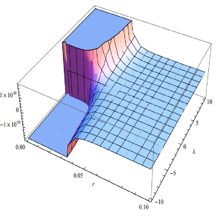
A conclusion that follows from these figures is that the cosmic string total energy $E$ per unit length in the z direction is essentially non-zero for small radius of the cosmic string. Moreover, this energy, which is not too sensitive to the variation of cosmic time, increases strongly with the increase of the parameter $\lambda$ of the chosen $f(T)$ model.

5 Conclusion

In this paper we have obtained a general expression for the Laudau-Lifshitz energy-momentum complex in the realm of Teleparallel modified gravity, the so called $f(T)$ theory (in analogy to the $f(R)$ theories). Such an expression has never appeared in the literature. The corresponding energy density has been evaluated for three plane symmetric metrics. For the first vacuum solution which has vanishing scalar torsion, the energy density is well defined and can vanish for certain $f(T)$ models. The second vacuum solution also with vanishing scalar torsion is characterized by a vanishing energy density in Teleparallel theory as in $f(T)$ theory. These results are totally different from those obtained in GR by using the same metrics. The last vacuum metric has constant scalar torsion and contributes to a well defined generalized energy density in $f(T)$ theory. An application has been made for an important Born-Infeld model satisfying weak energy condition.

In the second part of cosmological application of Laudau-Lifshitz energy-momentum complex in this this work, we have evaluated the energy density for a non-static cosmic string space-time. By considering a quadratic $f(T)$ model, we have found the energy distribution of thin cosmic strings according to our plotting results. It is an energy per unit length in the $z$ direction which depends on the radius $r$ and the unitary mass $M$ of the cosmic string. This energy increases considerably with the parameter of the considered quadratic $f(T)$ model.

References

• [1] C. W. Misner, K. S. Thorne and J. A. Wheeler, Gravitation (Freeman W.H. and Co., NY) 603 (1973).
• [2] A. Trautman, Gravitation: An Introduction to Current Research, ed. L. Witten (Wiley, 1962).
• [3] F.I. Cooperstock and R.S. Sarracino, J. Phys. A11 877 (1978)
• [4] H. Bondi, Proc. R. Soc. London A427, 249 (1990)
• [5] C. MΓΈller, Ann. Phys. (NY) 427 4, 347 (1958); Ann. Phys. (NY) 12, 118 (1961)
• [6] R.C. Tolman, ”Relativity, Thermodinamics and Cosmology” (Oxford Univ. Pres. London), 227 (1934)
• [7] L.D. Landau and E.M. Lifshitz, ”The Classical theory of fields” (Pergamon Press, Oxford, 1987) (Reprinted in 2002)
• [8] A. Papapetrou, Proc. R. Irish. Acad. A52, 11 (1948)
• [9] P.G. Bergmann and R. Thomson, Phys. Rev. 89, 400 (1953)
• [10] S. Weinberg, ”Gravitation and Cosmology: Principle and Applications of General Theory of Relativity” (John Wiley and Sons, Inc., New York) (1972)
• [11] A. Qadir and M. Sharif, Phys. Lett. A167, 331 (1992)
• [12] F.I. Mikhail, M.I. Wanas, A. Hindawi and E.I. Lashin, Int. J. Theor. Phys. 32, 1627 (1993)
• [13] T. Vargas, Gen. Rel. Grav.36, 1255 (2004)
• [14] Virbhadra, K. S. (1999). Phys. Rev. D60, 104041.
• [15] Chang, C.C., Nester, J.M. and Chen, C.: Phys. Rev. Lett.83 (1999)1897.
• [16] Tryon, E. P. (1973). Nature 246, 396.
• [17] M.G. Albrow, Nature 241, 56 (1973).
• [18] Cooperstock, F. I.,and Israelit,M. (1993).
• [19] N. Rosen Gen. Rel. Grav.26, 3 (1994)
• [20] Prigogine, I., Geheniau, J., Gunzing, E., and Nardone, P. (1989). Gen. Rel. Grav.21, 767.
• [21] T. MultamΓ€ki, A. Putaja, I. Vilja and E. C. Vagenas., arXiv 0712.0276.
• [22] M. Sharif and F. Shamin arXiv:0912.3632
• [23] G.G.L. Nashed, Phys.Rev. D 66, 064015 (2002).
• [24] S. C. Ulhoa, E. P. Spaniol., arXiv1303.144
• [25] R. Aldrovandi and J. G. Pereira, An Introduction to Gravitation Theory (preprint).
• [26] M. Salti, arXiv 0511095v4.
• [27] I. RADINSCHI and B. CIOBANU, Rom. Journ. Phys. 51, 3–4, p. 329–337, Bucharest, 2006
• [28] de Andrade, V. C. and Pereira, J. G. (1997). Phys. Rev. D 56, 4689.
• [29] Hayashi, K. and Shirafuji, T.: Phys. Rev. D19 (1979)3524.
• [30] F. Hehl, P. Von Der Heyde, G. Kerclok and J. Nester, General Relativity with Spin and Torsion: Foundation and Prospects, Rev. Mod. Phys. 48 (1976)393 [INSPIRE]
• [31] de Andrade, V. C., Guillen, L. C. T., and Pereira, J. G. (2000). Phys. Rev. Lett.84, 4533.
• [32] A. Sezgi, H. Baysal, Ismail Tarhan., Int J Theor Phys (2007) 46: 2607–2616
• [33] M. Salti, arXiv 0506061
• [34] L.L. So, J.M. Nester, On source coupling and the teleparallel equivalent to GR, arXiv:gr-qc/0612062.
• [35] A. V. Kpadonou, M. J. S Houndjo, M. E. Rodrigues [arXiv:1509.0877[gr-qc]]
• [36] M. Ganiou, Ines G. Salako M. J. S Houndjo J. Tossa [arXiv:1512.04801 [physics.gen-ph]]
• [37] Virbhadra, K. S. (1990). Phys. Rev. D41, 1086; Virbhadra, K. S. (1990). Phys. Rev. D 42, 1066;
• [38] Bertolami, O. and Sequeira, M.C.: arXiv:0903.4540v1.
• [39] R. Ferraro and F. Fiorini, Phys. Rev. D78, 124019 (2008)
• [40] Di Liu and M.J. RebouΓ§as arXiv:1207.1503
• [41] Matthew DePies arXiv 0908.3680v1
• [42] An Overview and Comparison by Dr. David Lewis Anderson.
• [43] Abbassi, A.M., Mirshekari, S. and Abbassi, A.H.: D78 (2008)064053.
• [44] Nashed, G.G.L., et al.: arXiv:1411.3293 (2014)
• [45] Bamba, K., et al.: Phys. Lett. B 731, 257 (2014a)
• [46] M.G. Ganiou C.AΓ―namon, M.J.S. Houndjo, and J. Tossa, Eur. Phys. J. Plus (2017) 132: 250
• [47] Nottale, L.: Found. Sci.15, 101.152 (2008)