Neutrinos in Large Extra Dimensions and Short-Baseline $\nu_{e}$ Appearance

Abstract

We show that, in the presence of bulk masses, sterile neutrinos propagating in large extra dimensions (LED) can induce electron-neutrino appearance effects. This is in contrast to what happens in the standard LED scenario and hence LED models with explicit bulk masses have the potential to address the MiniBooNE and LSND appearance results, as well as the reactor and Gallium anomalies. A special feature in our scenario is that the mixing of the first KK modes to active neutrinos can be suppressed, making the contribution of heavier sterile neutrinos to oscillations relatively more important. We study the implications of this neutrino mass generation mechanism for current and future neutrino oscillation experiments, and show that the Short-Baseline Neutrino Program at Fermilab will be able to efficiently probe such a scenario. In addition, this framework leads to massive Dirac neutrinos and thus precludes any signal in neutrinoless double beta decay experiments.

I Introduction

Unambiguous measurements of neutrino oscillations in the past two decades have provided clear evidence that neutrinos have non-vanishing masses and that the mass eigenstates are non-trivial admixtures of the flavor eigenstates. In fact, it is well understood that there are two small but quite different mass splittings, leading to flavor oscillations at macroscopic distances. For neutrino energies in the range of a few MeV the smaller (“solar”) mass splitting $\Delta m^{2}_{21}$ induces neutrino oscillations for baselines of few hundred kilometers, while the larger (“atmospheric”) splitting $\Delta m^{2}_{31}$ would induce oscillations at baselines of about one kilometer. Moreover, the Pontecorvo-Maki-Nakagawa-Sakata (PMNS) neutrino mixing matrix Pontecorvo (1957); Maki et al. (1962) is found to have large off-diagonal entries, at variance with the quark Cabibbo-Kobayashi-Maskawa (CKM) mixing matrix that has only small off-diagonal entries.

Despite the well understood 3-neutrino paradigm, there are indications of neutrino oscillations at very short baselines, that would call for additional mass splittings, beyond the solar and atmospheric ones aforementioned. Perhaps the most intriguing is the one associated with $\bar{\nu}_{\mu}\to\bar{\nu}_{e}$ appearance at the LSND experiment Athanassopoulos et al. (1995, 1996); Athanassopoulos et al. (1998a, b); Aguilar-Arevalo et al. (2001), and its recent reincarnation at the MiniBooNE experiment Aguilar-Arevalo et al. (2012, 2013). MiniBooNE ran in both neutrino and antineutrino modes, and in each channel an excess was observed. In the neutrino mode, the excess was found mostly at low neutrino energies, below $475\,\mathrm{MeV}$, while in the antineutrino mode the excess events range from $200$ to about $1250\,\mathrm{MeV}$. If these anomalies were to be interpreted as neutrino oscillations, they would concurrently point to a much larger mass splitting $\Delta m^{2}\sim 1\,\mathrm{eV}^{2}$, and an effective mixing angle $\sin^{2}2\theta_{\mu e}=4|U_{e4}U_{\mu 4}|^{2}\sim 0.003$, where $U$ is the PMNS matrix with one additional sterile neutrino.

A different anomaly, dubbed “reactor antineutrino anomaly”, is associated with an apparent reduction of the flux of reactor electron anti-neutrinos with respect to its expected value Mention et al. (2011); Huber (2011), something that may be interpreted as neutrinos being converted into sterile neutrinos at short propagation distances. However, there has been some observation of isotope dependence of this flux reduction An et al. (2017) that, if verified, will weaken the case for eV sterile neutrinos as an explanation of the reactor anti-neutrino anomaly. On the other hand, there is a similar discrepancy between expected and observed electron-neutrino events in the calibration of Gallium experiments Bahcall et al. (1995); Giunti and Laveder (2011); Anselmann et al. (1995). Both Gallium and reactor anomalies, if interpreted via neutrino oscillations, point to sterile neutrinos with $\Delta m^{2}\sim 1$ eV² or higher and an effective mixing angle $\sin^{2}2\theta_{ee}=4|U_{e4}|^{2}\sim 0.1$.

Beyond these observational issues, the mechanism behind neutrino masses is still unknown. An interesting realization comes from models of flat large extra dimensions (LED), in which right-handed neutrinos are allowed to propagate in the bulk of the extra dimensions, while the Standard Model (SM) fermions are restricted to live in the 4-dimensional brane Arkani-Hamed et al. (2001); Dienes et al. (1999); Dienes and Sarcevic (2001); Dvali and Smirnov (1999); Barbieri et al. (2000); Davoudiasl et al. (2002); Machado et al. (2011); Berryman et al. (2016); Cao et al. (2004); Mohapatra and Perez-Lorenzana (2001). The neutrino Yukawa couplings become tiny due to a volume suppression, leading to naturally light Dirac neutrinos. As a by-product of this type of models, a tower of Kaluza-Klein (KK) sterile neutrinos arises with masses proportional to the inverse radius $R$ of the extra dimension. Only the lower mass states of the tower mix in a relevant way with the SM-like neutrinos. When $R\sim\mu m$, these states are at the eV scale and thus the anomalies observed in short-baseline oscillation experiments could in principle be a consequence of this neutrino mass generation mechanism.

Such mechanism in LED is quite appealing, and can lead to neutrino disappearance from oscillations into sterile neutrinos at short baseline experiments. However, it cannot explain $\nu_{\mu}\to\nu_{e}$ appearance effects Davoudiasl et al. (2002), as suggested by LSND and MiniBooNE data. Models with more sterile Dirac fermions or extra dimensions with different radii are proposed in Ref. Davoudiasl et al. (2002) for this. Adding Majorana mass terms Diego and Quiros (2008); Lukas et al. (2000); Agashe and Wu (2001); Caldwell et al. (2001); Lam (2002) may serve as an another direction to be fully explored. In this article, we shall consider the possibility of adding Dirac bulk mass terms for the sterile neutrinos to accommodate neutrino appearance effects. These bulk mass terms were introduced before, e.g. see Refs. Diego and Quiros (2008); Lukas et al. (2000); Agashe and Wu (2001), but here we show explicitly their effects on oscillations at short baselines, particularly for the $\nu_{\mu}\to\nu_{e}$ appearance mode. It is worth mentioning that the generation of neutrino masses in the deconstructed LED model with bulk mass terms is analogous to the clockwork mechanism for the obtention of the small neutrino Yukawa couplings Hambye et al. (2016). Importantly, the LED scenario with bulk masses, that will be called here “LED+”, leads to weak effects in the long-baseline neutrino experiments, but it can be tested in the future Short-Baseline Neutrino Physics Program (SBN) at Fermilab Antonello et al. (2015). It would also lead to signatures at the Katrin Experiment Angrik et al. (2005).

This article is organized as follows. In section II we define our framework. In section III we concentrate on the phenomenology of our model, evaluating the constraints from existing data and studying the possible explanations of the observed anomalies in neutrino oscillation experiments. We also estimate the impact of LED+ in future neutrino oscillation experiments. In section IV, we discuss the constraints from Higgs decays and cosmology. We reserve section V for our conclusions. In Appendix A we show an interesting correspondence of this model with the linear dilaton scenario while in Appendix B we present the details regarding the Minimal Flavor Violation (MFV) assumption that will be used in the analysis of the model. In Appendix C we present details useful for the estimate of the constraints coming from kinematical tests of neutrino masses.

II Neutrinos in LED with Dirac bulk masses

We consider a $5$-dimensional flat space compactified on a $S_{1}/Z_{2}$ orbifold, with three generations of right-handed neutrinos propagating in the bulk, and SM fermions restricted to the 4D brane. Regarding the SM singlets, it is more convenient to work on an “intermediate” mass basis in which the flavor mixing has already been diagonalized. In such basis, the kinetic and mass terms in the action are given by

$$S_{f}=\int d^{4}x\,dz\,\left[i\bar{\Psi}_{i}\Gamma^{A}\overset{\leftrightarrow}{\partial_{A}}\Psi_{i}-c_{i}\bar{\Psi}_{i}\Psi_{i}\right],$$ (1)

with $\Gamma^{A}=(\gamma^{\mu},i\gamma^{5})$, $z\in[0,\pi R]$ and $c_{i}$ being the bulk mass parameters. Note that lepton number is conserved in our Lagrangian, so no Majorana mass term is present. Here we will use $\alpha,\beta$ to denote flavor, $i,j$ for the “intermediate” mass basis, and $n,m$ will be reserved to specify the KK-mode. The 5D fermion $\Psi_{i}$ can be decomposed as

$$\Psi^{L,R}_{i}=\sum_{n}\psi^{L,R}_{i,n}(x)f^{L,R}_{i,n}(z),$$ (2)

with $\Psi^{L,R}_{i}=P_{L,R}\Psi_{i}$ and $\gamma_{5}\Psi^{L,R}_{i}=\mp\Psi^{L,R}_{i}$. To have the Dirac action canonically normalized in four dimensions, the wave functions $f^{L,R}_{i,n}(z)$ should satisfy the following normalization condition

$$\int^{\pi R}_{0}dz\,f^{L,R}_{i,n}(z)f^{L,R}_{i,m}(z)=\delta_{mn}.$$ (3)

The orbifold symmetry allows two choices of boundary conditions Ponton (2013): either all left-chiral fields are odd functions (Dirichlet boundary conditions) and all right-handed ones are even functions, or vice-versa. In order to generate neutrino masses, there should be a right-handed chiral zero mode, therefore we will use the Dirichlet boundary conditions for the left-handed modes on both branes. Then, we get a right-handed massless zero mode with wave function

$$f^{R}_{i,0}(z)=\sqrt{\frac{2c_{i}}{e^{2\pi Rc_{i}}-1}}e^{c_{i}z},$$ (4)

while for all other KK-modes we obtain

$$f^{L}_{i,n}(z)=\sqrt{\frac{2}{\pi R}}\sin\left(\frac{nz}{R}\right),$$ (5)

$$f^{R}_{i,n}(z)=\sqrt{\frac{2}{\pi R\,m_{i,n}^{2}}}\left[c_{i}\sin\left(\frac{nz}{R}\right)+\frac{n}{R}\cos\left(\frac{nz}{R}\right)\right],$$ (6)

$$(m^{i}_{n})^{2}=\Big{(}\frac{n}{R}\Big{)}^{2}+c_{i}^{2}.$$ (7)

The bulk fermions will couple to SM neutrinos through the Yukawa terms in the IR brane Grossman and Neubert (2000). In the “intermediate” basis, the Yukawa terms read

$$S_{Y} =-\int d^{4}x\sum_{i=1}^{3}\left(y_{i}\bar{L}_{i}\tilde{H}\Psi^{R}_{i}(x^{\mu},0)+\text{h.c.}\right)$$ (8)

$$=-\int d^{4}x\sum_{i=1}^{3}\sum_{n=0}^{\infty}\left(Y^{i}_{n}\bar{L}_{i}\tilde{H}\psi_{i,n}^{R}(x^{\mu})+\text{h.c.}\right),$$

with $\tilde{H}=i\sigma_{2}H^{\ast}$ and the effective coupling $Y^{i}_{n}=y_{i}f^{R}_{i,n}(0)$. We define $y_{i}=\lambda^{i}/\sqrt{M_{5}}$ with $M_{5}$ the fundamental scale of the extra dimensional theory and $\lambda^{i}$ being free dimensionless parameters. $M_{5}$ is related to the Planck scale by

$$M_{\text{Pl}}^{2}=M_{5}^{2+d}V_{d},$$ (9)

where $d$ is the number of extra dimensions and $V_{d}$ is their volume. Note that to have both the 5D Yukawa matrix and the singlet bulk mass matrix diagonalized in the “intermediate” basis, we have assumed alignment between these two matrices that is equivalent to assume a Minimal Flavor Violation (MFV) scenario (see Appendix B for details). This assumption is not essential for this scenario to work, but it will greatly simplify the phenomenological analysis. For simplicity, the Yukawas and the bulk masses in the intermediate basis are taken to be real. Therefore, there are no additional CP phases besides the standard $\delta_{CP}$ appearing in a 3-neutrino framework.

We define the relation between the flavor and “intermediate” bases as in Machado et al. (2011), namely

$$\nu_{\alpha,0}^{L}=U_{\alpha i}\,\nu_{i,0}^{L},\quad\Psi_{\alpha}=R_{\alpha i}\Psi_{i}.$$ (10)

In the above, $U_{\alpha i}$ is the PMNS matrix for the standard three flavor neutrino model and $R$ is a matrix that diagonalizes the bulk masses and Yukawa couplings. The mass matrix $M_{i}^{nm}$ in the intermediate basis reads

$$M_{i}=\begin{pmatrix}vY^{i}_{0}&0&\cdots&0\\ vY^{i}_{1}&m^{i}_{1}&\cdots&0\\ \vdots&0&\ddots&0\\ vY^{i}_{n}&0&\cdots&m^{i}_{n}\end{pmatrix},$$ (11)

where $v=174~{}\mathrm{GeV}$ is the Higgs vev.

For one extra dimension, the Yukawa couplings of the zero and KK-modes are given by

$$Y^{i}_{0} =\lambda^{i}\sqrt{\frac{2}{M_{5}}}\sqrt{\frac{c_{i}}{e^{2c_{i}\pi R}-1}},$$

$$Y^{i}_{n} =\lambda^{i}\sqrt{\frac{2}{M_{5}\pi R}}\sqrt{\frac{n^{2}}{n^{2}+c_{i}^{2}R^{2}}}.$$ (12)

We are interested in sterile neutrinos with masses of the order of 1 eV, implying at least one extra dimension with size $1/R={\cal{O}}$(1 eV). If this were the only extra dimension, consistency with Eq. (9) would demand $M_{5}\simeq 10^{10}$ GeV, and hence values of $\lambda_{i}={\cal{O}}(10^{-4})$ would be necessary in order to obtain the correct active neutrino masses for $c_{i}={\cal{O}}$(1/R). Alternatively, one can think of models in which neutrinos propagate in $d$ extra dimensions, where the size of the additional extra dimensions is much smaller than $R$, $R_{k>1}\ll R_{1}\sim R$. In such a case, under the assumption that the effects of the heavier KK modes from the extra dimensions with small radii $R_{k>1}$ can be neglected, one obtains

$$Y^{i}_{0} =\lambda^{i}\sqrt{\frac{2}{M_{5}^{d}V_{d}}}\sqrt{\frac{c_{i}\pi R}{e^{2c_{i}\pi R}-1}}=\lambda^{i}\frac{M_{5}}{M_{pl}}\sqrt{\frac{2c_{i}\pi R}{e^{2c_{i}\pi R}-1}},$$

$$Y^{i}_{n} =\lambda^{i}\sqrt{\frac{2}{M_{5}^{d}V_{d}}}\sqrt{\frac{n^{2}}{n^{2}+c_{i}^{2}R^{2}}}=\lambda^{i}\frac{M_{5}}{M_{pl}}\sqrt{\frac{2n^{2}}{n^{2}+c_{i}^{2}R^{2}}},$$ (13)

To derive the second equality in Eq. (13) we have used Eq. (9). We can now lower the value of $M_{5}$ in order to obtain values of $\lambda_{i}={\cal{O}}(1)$. In our scenario with small bulk mass terms, for definiteness, we fixed $M_{5}=10^{6}$ GeV. Note that with more than one extra dimension, we require not only Dirichlet boundary conditions for the left-handed modes, but also that the derivative of the right-handed bulk fermion wavefunction with respect to coordinates in $R_{k>1}$ directions are zero at the boundaries. The boundary condition applied in this way would allow for only one zero mass mode with the wavefunction given above.

We define the left rotation that diagonalizes the mass matrix $M_{i}$ in the intermediate basis as

$$W_{i}^{nn^{\prime}}(M_{i}M_{i}^{\dagger})^{n^{\prime}m^{\prime}}W_{i}^{mm^{\prime}}=m^{2}_{i,n}\delta_{nm},$$ (14)

where $m^{2}$ is a diagonal matrix in KK space. Thus, the final left rotation involving active neutrinos that diagonalizes the full mass matrix is given by

$$\mathcal{U}_{\alpha i}^{0n}=U_{\alpha i}W_{i}^{0n}.$$ (15)

Note that the other entries of $\mathcal{U}_{\alpha i}^{nm}$ are not observable, as the sterile neutrinos do not couple to the electroweak gauge bosons. The oscillation amplitude among active neutrinos is given by

$$\mathcal{A}(\nu_{\alpha,0}\to\nu_{\beta,0};L)=\sum_{i,n}\mathcal{U}_{\alpha i}^{0n}(\mathcal{U}_{\beta i}^{0n})^{*}\exp\left(i\frac{m_{i,n}^{2}L}{2E}\right),$$ (16)

where $L$ is the experiment baseline, $E$ is the neutrino energy, and the superscripts indicating left-handedness have been dropped. In our numerical simulations, we shall include the matter effects by adopting a similar procedure as the one in Refs. Barbieri et al. (2000); Davoudiasl et al. (2002); Machado et al. (2011), namely, we rotate the matter potential into the intermediate basis and include its effects in the diagonalization of the KK modes.

Since the PMNS matrix has been fairly well constrained from neutrino oscillation experiments, the effects of the KK modes can only be a perturbation over the standard three neutrino scenario. Therefore the $3\times 3$ block $\mathcal{U}_{\alpha i}^{00}$ would present a slight deviation from unitary. To connect this discussion more concretely with current neutrino data, first we note that the measured atmospheric and solar mass squared splittings correspond to $\Delta m^{2}_{\rm atm}\simeq m_{3,0}^{2}-m_{1,0}^{2}$ and $\Delta m^{2}_{\odot}\simeq m_{2,0}^{2}-m_{1,0}^{2}$, respectively. Moreover, the observed approximate unitarity of the PMNS matrix Parke and Ross-Lonergan (2016), requires the deviations from unitarity to be at most about 10%. That translates into a bound

$$\sum_{i=1}^{3}|\mathcal{U}_{\alpha i}^{00}|^{2}\gtrsim 0.9$$ (17)

for each flavor $\alpha$. In Fig. 1 we present isocontours of the masses of the 0-mode (red) and 1-mode (dashed blue) in the radius $R$ vs. $cR$ plane. The case $c=0$ is the LED scenario without bulk mass term, while $R\to 0$ should recover Dirac neutrinos with the standard 3-neutrino framework. In the whole parameter space shown, the approximate bound from Eq. (17) is satisfied.

Based on Fig. 1, we define three benchmark points listed in Table 1 that will be used later on to perform a phenomenological study of the model. Point 1 realizes the normal ordering of the left-handed neutrinos, presenting relatively light KK modes with sizable mixing to the active neutrinos. In point 2, on the other hand, active neutrinos have inverted mass ordering, while the first KK mode masses are below 1 eV and the KK mixing is small. Finally, point 3 presents a degenerate neutrino spectrum (normal ordering) with KK modes around the eV scale and with large mixing to active neutrinos. A distinctive feature between LED without bulk masses and LED+ is the relation between KK mixing and the masses of active neutrinos and KK modes. In LED without bulk masses, the heavier the active neutrino is, the larger is the mixing with KK modes, as explicitly shown later on in Eq. (18). Moreover, the first KK modes in each tower necessarily have the larger mixings with the active neutrinos (as exemplified in Eq. (18) and by the crosses in Fig. 2). In LED+ instead, the presence of non-zero $c_{i}$’s can dramatically change the above behaviors. To exemplify the first, we present point 2 in Table 1, where the lightest active neutrino has the largest mixing with the KK modes. For the latter, the turquoise circles in Fig. 2 demonstrate that a non-zero $c_{i}$ can significantly suppress the mixing between active neutrinos and the first KK modes.

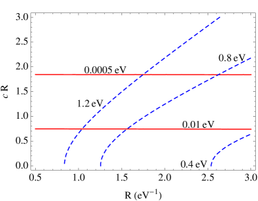
Figure 1: The mass of the zero mode (red lines) and of the first KK mode (dashed-blue lines) as a function of the radius R and the bulk mass $c$ times $R$. We fix the scale $M_{5}=10^{6}~{}\text{GeV}$, $\lambda_{i}=0.66$.

$\{P_{a},\,\nu_{i}$}	$\dfrac{R}{{\rm eV}^{-1}}$	$c_{i}\,R$	$\lambda^{i}$	$\dfrac{m^{2}_{i,0}}{{\rm eV}^{2}}$	$\dfrac{m^{2}_{i,n^{\prime}}}{{\rm eV}^{2}}$	$|W^{0n^{\prime}}_{i}|^{2}$
{$P_{1}$, $\nu_{1}$}	$1.9$	$4.24$	$0.42$	$\approx 0$	$9.3$	$9.0\cdot 10^{-5}$
{$P_{1}$, $\nu_{2}$}	$1.9$	$1.19$	$2.0$	$7.6\cdot 10^{-5}$	$0.66$	$0.0196$
{$P_{1}$, $\nu_{3}$}	$1.9$	$-0.037$	$0.66$	$2.5\cdot 10^{-3}$	$0.27$	$0.0169$
{$P_{2}$, $\nu_{1}$}	$6.4$	$-1.1$	$0.27$	$2.5\cdot 10^{-3}$	$0.056$	$5.9\cdot 10^{-3}$
{$P_{2}$, $\nu_{2}$}	$6.4$	$-1.2$	$0.25$	$2.6\cdot 10^{-3}$	$0.066$	$3.8\cdot 10^{-3}$
{$P_{2}$, $\nu_{3}$}	$6.4$	$3.2$	$1.1$	$\approx 0$	$0.64$	$0.01$
{$P_{3}$, $\nu_{1}$}	$1.8$	$0.43$	$0.42$	$1.9\cdot 10^{-4}$	$0.37$	$4.4\cdot 10^{-3}$
{$P_{3}$, $\nu_{2}$}	$1.8$	$1.0$	$2.4$	$2.6\cdot 10^{-4}$	$0.65$	$0.0361$
{$P_{3}$, $\nu_{3}$}	$1.8$	$0.41$	$1.7$	$2.7\cdot 10^{-3}$	$0.37$	$0.0576$

Table 1: Benchmark points used in the simulation, where $P_{a}$ for $a=\{1,2,3\}$ means point 1, 2, 3. The index $i$ is the “intermediate basis” index, we fixed $M_{5}=10^{6}~{}\mathrm{GeV}$ and the index $n^{\prime}$ represents the KK mode that has the largest mixing with active neutrinos.

III Neutrino phenomenology

The phenomenology of neutrinos in large extra dimensions was widely studied for models without bulk mass terms (see e.g.Davoudiasl et al. (2002); Machado et al. (2011, 2012); Basto-Gonzalez et al. (2013); Berryman et al. (2016); Adamson et al. (2016)). In these realizations, the most striking signature is the disappearance of active neutrinos in short baseline oscillation experiments with a very regular pattern of masses and mixings. The appearance mode is however absent in such studies precisely due to the regular behaviour of the KK spectrum and the structure of the mixing angles. In particular, there is sizable mixing among flavors of the same KK mode (say, “horizontally”), or among different KK modes of the same flavor (“vertically”). “Diagonal” mixing, that is, between different KK modes of different flavors is practically absent. Moreover, the “horizontal” mass splittings are always close to the atmospheric or solar mass splittings, and thus cannot mediate, e.g., $\nu_{\mu}\to\nu_{e}$ appearance at short baselines as suggested by the LSND and MiniBooNE anomalies.

To see this explicitly, we calculate the expression for Eq. (16) in the limit $c_{i}=0$. Using Eq. (7) and the approximation

$$W^{0n}_{i}\sim\frac{vY^{i}_{n}}{m^{i}_{n}}\sim\frac{\sqrt{2}m_{i,0}}{(n/R)},$$ (18)

for $n>0$, and $W_{i}^{00}\sim 1$, we have

$$\mathcal{A}(\nu_{\alpha,0}\to\nu_{\beta,0};L)\sim\sum_{i=1}^{3}U_{\alpha i}U_{\beta i}^{*}\exp\left(i\frac{\Delta m^{2}_{i,0}L}{2E}\right)$$

$$+2\sum_{i=1}^{3}\sum_{n=1}^{\infty}U_{\alpha i}U_{\beta i}^{*}\frac{m_{1,0}^{2}}{(n/R)^{2}}\exp\left(i\frac{n^{2}L}{2R^{2}E}\right)$$

$$+2\sum_{i=2,3}\sum_{n=1}^{\infty}U_{\alpha i}U_{\beta i}^{*}\frac{\Delta m^{2}_{i,0}}{(n/R)^{2}}\exp\left(i\frac{n^{2}L}{2R^{2}E}\right)$$ (19)

with $\Delta m^{2}_{i,0}=m^{2}_{i,0}-m^{2}_{1,0}$ for $i=2,3$ to be the solar and atmospheric mass splitting, respectively. The first term in this approximation gives the standard 3-active neutrino oscillation result. For the appearance mode, $\alpha\neq\beta$, the second term vanishes, due to the unitarity of the PMNS matrix, and the third term contribution is suppressed by $\Delta m_{i,0}^{2}R^{2}$, as pointed out in Ref. Davoudiasl et al. (2002).

The presence of bulk mass terms leads to a qualitatively different picture. As can be seen in Eqs. (7) and (12), a non-zero $c_{i}$ will perturb the regularity of the masses in the corresponding KK tower, therefore enlarging the “horizontal” splittings for $n\geq 1$. To exemplify this effect we show in Fig. 2 the masses and mixings $|W^{0n}_{i}|^{2}$ between neutrino $\nu_{i,0}$ and the $n^{\text{th}}$ KK-mode for the benchmark point 1 (see Table 1) and $i=1,2$. Moreover, in Fig. 3 we show how the masses of the first three KK modes and their mixings with $\nu_{i,0}$ change as a function of $c_{i}R$. Notice that not only the KK mode mass but also the mixing with active neutrinos changes drastically for different values of the bulk masses. As it is shown in Fig. 3, for increasing values of the bulk masses, the mixing with the first KK modes can be suppressed, thus enhancing the relative importance of the heavier modes.

The upper panel of Fig. 4 shows the oscillation probabilities at short baselines for the three benchmark points given in Table 1. As can be clearly seen from Fig. 4, bulk mass terms can lead to appearance at short-baseline neutrino experiments, possibly providing an explanation for the LSND and MiniBooNE anomalies.

We also expect that LED+ scenarios may have an impact in long-baseline oscillation experiments. The best way to look for heavy KK mode effects in long-baseline experiments would be in $\nu_{\mu}$ disappearance, as $\nu_{\mu}\to\nu_{e}$ appearance is suppressed by $\theta_{13}$ and also depends on $\delta_{CP}$ and the mass ordering. The LED+ effects on disappearance experiments yield fast oscillations that translate into an overall normalization change. For heavier KK modes, oscillations will also happen at the near detector and their effect will partially cancel in the near-to-far ratio Bhattacharya et al. (2012). In the lower panel of Fig. 4 we illustrate the $\nu_{\mu}$ disappearance effects in long-baseline experiments by showing the ratio of $\nu_{\mu}\to\nu_{\mu}$ oscillation probabilities between the near and far detectors. Notice that point 1 leads to a smaller effect due to the fact that active neutrinos mix with less KK modes compared to point 2 because of different values of $c_{i}$ and has a smaller mixing with a single KK mode compared to point 3.

We would also like to point out two important effects that should be taken into account when calculating the oscillation probabilities. First, the absolute values of $\Delta m^{2}_{31}$ should be slightly different between normal (points 1 and 3) and inverted hierarchy (point 2) cases in order to get the minimum of the oscillation at the same energy. This is due to the fact that the quantity that is measured in the $\nu_{\mu}\to\nu_{\mu}$ channel is the so-called $|\Delta m^{2}_{\mu\mu}|$, which is a function of the atmospheric and solar splittings, as well as the PMNS mixing angles. See Ref. Nunokawa et al. (2005) for detailed explanations. Second, to obtain percent level precision, for all benchmark points chosen, one needs to consider about 20 KK modes. This contrasts strongly with the LED scenario without bulk mass terms, in which 5 or 6 KK modes are enough to get to percent level precision calculations.

Below, we will analyze the current constraints coming from MINOS/MINOS+, NO$\nu$A, T2K, short baseline reactor experiments, LSND and MiniBooNE, as well as the future sensitivity of DUNE and the Short Baseline Neutrino Program at Fermilab. In principle, the IceCube experiment could also set a strong constraint on sterile neutrino models Aartsen et al. (2016) via a MSW resonance that would enhance active to sterile conversion when neutrinos cross the core of the Earth Nunokawa et al. (2003). Nevertheless, we do not consider the IceCube sensitivity here for the following reason. As can be seen in Ref. Adamson et al. , IceCube and MINOS/MINOS+ have comparable sensitivities to constrain sterile neutrinos with $\Delta m^{2}\sim 1~{}$eV². Nevertheless, for values of $\Delta m^{2}$ larger than $\sim 1~{}$eV², the sensitivity of IceCube degrades quickly, as the MSW resonance moves to higher energies for which the flux of atmospheric neutrinos becomes smaller. Since in our scenario it is typical that many KK modes above 1 eV have sizeable contributions to the oscillation probability, we expect the IceCube bound to be weaker than MINOS/MINOS+. Therefore, in this work we shall concentrate on accelerator and reactor oscillation experiments only.

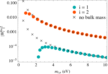
Figure 2: Pattern of KK masses and mixings for the benchmark point 1 in Table 1 with $i=1$ (turquoise) and $i=2$ (red). For comparison, we also present the equivalent pattern for LED without bulk mass terms (crosses).

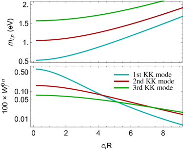
Figure 3: Masses and mixings with active neutrinos of the first three KK modes as a function of the bulk mass parameter times the radius of the extra dimension, $c_{i}R$. The other LED+ parameters are taken to be $R=1.9$ eV^-1, $\lambda_{i}=2.0$ and $M_{5}=10^{6}$ GeV.

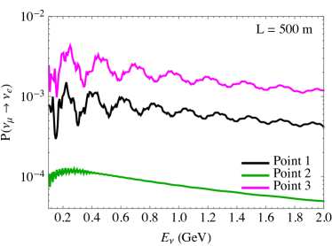
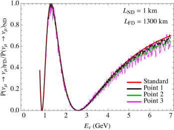
Figure 4: Oscillation probabilities for the three benchmark points given in Table 1 for short and long baselines as indicated in the plots. In the lower panel, the ratio of far-to-near detector probabilities is presented.

III.1 Past and present oscillation experiments

III.1.1 MINOS and MINOS+

The standard LED scenario can be probed at long-baseline neutrino oscillation experiments. The recent MINOS analysis Adamson et al. (2016) using data collected from 2005 to 2012 excludes large extra dimension models with $R>(0.5\,\mathrm{eV})^{-1}$ at $90\%$ C.L., for a massless lightest neutrino. In addition, it is expected that MINOS+ will have a similar sensitivity to probe large extra dimension models Adamson et al. . As explainied above, the LED+ effects on disappearance experiments yield fast oscillations that translate into an overall normalization change. The experimental sensitivity will therefore be limited by the overall normalization uncertainty which is about 5% Adamson et al. (2016).

To estimate the MINOS and MINOS+ sensitivity to LED+ models, we consider the combined flux, assuming $10.71\times 10^{20}$ and $5.8\times 10^{20}$ POT for the low and high energy beam configurations, respectively. The energy resolution and efficiency were taken from Vahle . In Fig. 5, we illustrate the LED+ effects for the three benchmark points (Table 1) which have $R^{-1}$ between $1.4-6.5~{}\mathrm{eV}$. We show the near-to-far $\nu_{\mu}\to\nu_{\mu}$ ratios (normalized to 1 in the absence of oscillations) together with a 5% normalization uncertainty (light red band) and the corresponding statistical uncertainty (light blue band) assuming full run Adamson et al. (2016). Note that the normalization uncertainty is fully correlated among energy bins, so it only applies to smeared fast oscillations, which is the case for the three benchmark points. The benchmark points 1, 2, and 3 are depicted as the black, green and magenta lines, respectively. The first two are consistent within errors with the standard three flavor neutrino prediction (red line), while point 3 is marginally consistent (see also Fig. 11 later on).

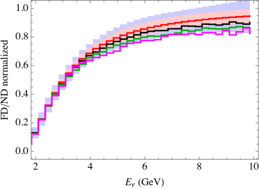
Figure 5: Near-to-far ratio of events for the $\nu_{\mu}\to\nu_{\mu}$ disappearance channel at MINOS and MINOS+, normalized to 1 in the absence of oscillations. The red line is the expected ratio for the standard 3-neutrino framework. The light red band shows a 5% systematic uncertainty, while the blue band corresponds to the statistical uncertainty assuming full run Adamson et al. (2016). Black, green and magenta are the ratios for points 1, 2 and 3, respectively.

III.1.2 NO$\nu$​A and T2K

The current NO$\nu$A and T2K experiments may also constrain large extra dimension scenarios. Their sensitivity to LED without bulk masses was estimated in Ref. Machado et al. (2011): no improvement over MINOS sensitivity would be achieved. The reason is the following. The effects of KK mode oscillations in the $\nu_{\mu}\to\nu_{\mu}$ channel are more sizable at higher energies away from the atmospheric minimum. However, NO$\nu$A and T2K are narrow band beam experiments, having the neutrino spectrum very localized at the atmospheric minimum. Although this improves the sensitivity to the standard 3-neutrino oscillation parameters, it degrades the sensitivity to LED.

To exemplify the impact of LED+ in these experiments, we present in Fig. 6 the near-to-far ratio of events in NO$\nu$A (normalized to 1 in the absence of oscillations) for $3\times 10^{21}$ protons on target, and 14 kton fiducial mass Messier (1999); Paschos and Yu (2002); Ambats et al. (2004); Yang and Woijcicki (2004) for the three benchmark points. Points 1, 2, and 3 are depicted by the blue, green and magenta histograms, respectively, while the red line corresponds to the standard 3-neutrino scenario. Both systematic (5%) and statistical uncertainties are shown as the red and blue bands, respectively. Notice that Fig. 6 only depicts neutrino energies lower than about 3.5 GeV, since above those energies the statistical error is fairly large due to the narrow band beam that peaks at the atmospheric oscillation minimum, as discussed above. Large deviations from the standard neutrino oscillation scenario happen at high energies, see Fig. 4, not shown in Fig. 6, and hence NO$\nu$A has limited sensitivity to test our benchmark LED+ scenarios. One could wonder about what happens to the appearance channel, since LED+ may induce non-negligible $\nu_{\mu}\to\nu_{e}$ transitions. However, the appearance channel has low statistics and a strong dependence on $\theta_{23}$, $\delta_{CP}$ and the mass ordering, hence it is not expected to put any competitive bound on LED+. The same features are present in T2K, and therefore we do not expect either of these two experiments to substantially improve MINOS and MINOS+ sensitivities to the LED+ scenario.

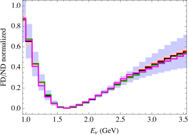
Figure 6: Near-to-far ratio of events for the $\nu_{\mu}\to\nu_{\mu}$ disappearance channel at NO$\nu$A, normalized to 1 in the absence of oscillations. The red line is the expected ratio for the standard 3-neutrino framework. The light red band shows a 5% systematic uncertainty, while the blue band corresponds to the statistical uncertainty assuming $3\times 10^{21}$ protons on target. Black, green and magenta are the ratios for points 1, 2 and 3 in Table 1, respectively.

III.1.3 Reactor experiments and the Gallium anomaly

The reactor antineutrino anomaly is a discrepancy between observed and predicted reactor antineutrino fluxes. At present, based on Refs. Mention et al. (2011); Huber (2011), the measured neutrino flux at short baseline reactor experiments is 6% below the theoretical flux prediction, with an associated uncertainty of about 2%. Recently, the Daya Bay analysis on the flux isotope dependence has shown that most of this discrepancy comes from the ²³⁵U isotope Giunti (2017); An et al. (2017). Besides, other authors have proposed the use of a larger, more conservative theoretical uncertainty of $5\%$, based on considerations of nuclear effects Hayes and Vogel (2016). While this challenges the theory prediction for the fluxes and its associated uncertainties, the solution to the reactor anomaly puzzle is still far from clear. Here, we adopt an agnostic perspective and show the sensitivity of short baseline reactor neutrino experiments to LED+.

As it has been shown in Ref. Machado et al. (2012), the reactor anomaly could in principle be explained by LED models via $\bar{\nu}_{e}$ mixing with KK modes. Similarly, this could also be explained in LED+ models. We present in Fig. 7 the predicted ratio of events between our scenario and no oscillations (as is the case for the standard 3 neutrino framework) for the three benchmark points in Table 1 and a representative baseline of $L=10\,\mathrm{m}$. The ratio between the total number of observed to expected events is depicted by the orange dashed line, with a 5% associated theoretical uncertainty (light red band). Point 1 leads to 5% disappearance ratio, point 2 allows for about 3%, while point 3 shows around 10% disappearance in $\bar{\nu}_{e}$. Therefore, taking the aforementioned 2% theoretical error on the flux prediction, point 1 could in principle explain the reactor anomaly, point 2 would predict too little disappearance, while point 3 would predict a slightly larger suppression of the flux. If the theoretical error were taken to be larger, for instance 5% Hayes and Vogel (2016), then all three points would be in agreement with the reactor data.

In a similar fashion, the Gallium anomaly is a discrepancy between the measured and theoretically predicted number of $\nu_{e}$ events in solar neutrino calibration experiments Hampel et al. (1998); Kaether et al. (2010); Abdurashitov et al. (1999, 2006). There, $\nu_{e}$ is emitted by a radioactive source and detected in a Gallium tank that contains the source. Although the $\nu_{e}$ flux is fairly well known, the detection cross section depends on nuclear physics form factors with relatively large uncertainties Bahcall (1997); Frekers et al. (2011). The ratio between measured and expected number of events is $R=0.84^{+0.054}_{-0.051}$ Kopp et al. (2013). Thus, points 1 and 2 are consistent with the Gallium anomaly within 2$\sigma$, while point 3 would provide a better fit to these experiments.

III.1.4 LSND and MiniBooNE

As we emphasized above, adding Dirac bulk mass terms splits the mass degeneracy between the three towers of KK modes and may lead to $\nu_{\mu}\to\nu_{e}$ appearance, thereby providing a possible explanation for the anomalies observed at LSND and MiniBooNE. We examined the event excess for the three benchmark points given in Table 1 in light of the full LSND Athanassopoulos et al. (1997); Aguilar-Arevalo et al. (2001) and MiniBooNE data Aguilar-Arevalo et al. (2012), as shown in Fig. 8. As we do not consider CP violation in the KK sector (we take all Yukawas and $c_{i}$ to be real), the appearance probabilities $\nu_{\mu}\to\nu_{e}$ and $\bar{\nu}_{\mu}\to\bar{\nu}_{e}$ are nearly identical (apart from the small impact of matter effects).

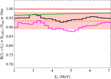
Figure 7: Ratio between LED+ and standard oscillations for $\bar{\nu}_{e}\to\bar{\nu}_{e}$ disappearance events at a reactor neutrino experiment for an illustrative baseline of 10 m. The orange dashed line is the ratio between the total number of observed to expected events. The light red band shows a 5% theoretical uncertainty. The red, black, green and magenta lines display the ratios for the standard scenario, and benchmark points 1, 2 and 3 in Table 1, respectively.

For LSND (upper panel), the background is shown as the shaded histogram. We see clearly that point 3 (magenta line) could explain the excess quite well, while point 1 (black line) gives rise to a smaller excess and point 2 (green line) essentially predicts no excess at all. We will discuss the impact of LED+ on MiniBooNE in a bit more detail. For the neutrino mode, points 1 (black), 2 (green) and 3 (magenta) yield approximately 65, 8, and 176 excess events, respectively, in the region with neutrino energy from $200~{}\mathrm{MeV}$ to $1200~{}\mathrm{MeV}$. For the antineutrino mode, the excess events are 33, 4, and 89, respectively. Point 2 predicts very little excess due the small active neutrino mixing with the KK modes and typically small $\Delta m^{2}_{KK}$ for the relevant modes, as can be seen in Table 1. Moreover, we notice that the excesses, for points 1 and 3, are found in the higher energy region, $E_{\nu}\sim 400-800$ GeV. This is due to the $\Delta m^{2}_{KK}$ which is typically at the eV² scale or larger. As a final comment, notice that to explain the LSND/MiniBooNE anomaly (point 3), we are slightly off the disappearance data as mentioned previously (see the magenta lines in Figs. 5 and 7). We would like to point out that this tension is a common feature of sterile neutrino models which try to address the LSND/MiniBooNE anomalies Kopp et al. (2013); Collin et al. (2016); Gariazzo et al. (2017). This originates in the fact that $\nu_{e}$ ($\nu_{\mu}$) disappearance depends on $4|U_{e4}|^{2}$ ($4|U_{\mu 4}|^{2}$) while the $\nu_{\mu}\to\nu_{e}$ appearance probability depends on $4|U_{e4}U_{\mu 4}|^{2}$, and thus a non-zero appearance excess necessarily implies relevant $\nu_{e}$ and $\nu_{\mu}$ disappearance as well.

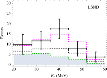
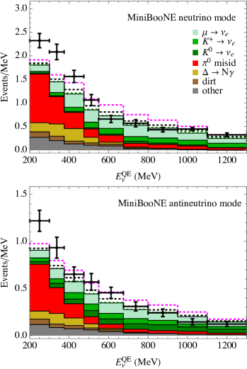
Figure 8: $\bar{\nu}_{e}$ appearance spectrum at LSND (top), and $\nu_{e}$ appearance MiniBooNE for the neutrino (middle) and antineutrino (bottom) modes. The shaded histograms are the different background components as indicated in the legend (taken from Ref. Aguilar-Arevalo et al. (2001) for LSND and Ref. Aguilar-Arevalo et al. (2012) for MiniBooNE). Black, green and magenta lines are for points 1, 2 and 3 in Table 1, respectively.

III.2 Future oscillation experiments

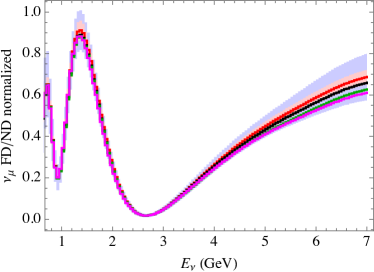
Figure 9: Near-to-far ratio for the $\nu_{\mu}\to\nu_{\mu}$ disappearance channel at DUNE. The red line is the expected ratio for the standard 3-neutrino framework. The light red (blue) band shows the 5% systematic (statistical) uncertainty assuming 3 years run. Black, green and magenta are the ratios for points 1, 2 and 3 in Table 1, respectively.

III.2.1 DUNE

The sensitivity of the Deep Underground Neutrino Experiment (DUNE) to LED models without bulk mass terms was estimated in Ref. Berryman et al. (2016): extra dimensions with $R\gtrsim(0.6~{}{\rm eV})^{-1}$ could be probed by DUNE for a massless lightest active neutrino. This sensitivity is similar to the current constraint coming from the MINOS experiment. In Fig. 9, we present the near-to-far event ratio, normalized to 1 in the absence of neutrino oscillations, for the DUNE experiment, assuming similar far and near detector acceptances, for the three benchmark points in our scenario. In our simulation we have used the energy resolution from Ref. De Romeri et al. (2016), of about 7% at high energies for $\nu_{\mu}$ charged current (CC) events, and the $\nu_{\mu}$ flux and CC cross section from Ref. Alion et al. (2016), together with a 5% normalization uncertainty.  We assume a running time of 3.5 years in neutrino mode and a detector of 40 kton fiducial mass. As expected, since the oscillation phase varies slower, deviations from standard oscillations are more easily observed at the high energy tail of the spectrum. Point 1 seems to be rather challenging to be tested at DUNE. Points 2 and 3 have the potential to be probed, but that requires a detailed statistical analysis. See for example the DUNE sensitivity to point 3 in Fig. 11. Nevertheless, as we shall discuss next, our model will likely be first probed by the Fermilab Short-Baseline Neutrino Program.

III.2.2 Short-Baseline Neutrino Program

The Short-Baseline Neutrino Program (SBN) at Fermilab consists of three detectors, LAr1-ND, MicroBooNE and ICARUS-T600 with a distance from the target of 110 m, 470 m and 600 m, respectively. The MicroBooNE experiment has started to take data and will be able to investigate the source of the excess observed by MiniBooNE. Sterile neutrino models that explain the MiniBooNE excess do not necessarily affect the oscillation spectrum at LAr1-ND. However, in the LED+ framework, towers of KK modes would contribute to the oscillation spectrum at LAr1-ND. As a comparison, we show in Fig. 10 the oscillation spectrum for the three benchmark points in LED+ and the best global fit point Kopp et al. (2013) in a $3+1$ sterile neutrino model which has $\Delta m_{41}^{2}=0.42$ eV², $\sin^{2}(2\theta_{\mu e})\equiv 4|U_{e4}U_{\mu 4}|^{2}=0.013$. We used a luminosity of $6.6\times 10^{20}$, $1.32\times 10^{21}$, and $6.6\times 10^{20}$ protons on target for LAr1-ND, MicroBooNE, and ICARUS-T600, respectively. The event numbers predicted at the three detectors for our benchmark points and the best-fit $3+1$ sterile neutrino model are listed in Table 2. By considering the spectra in Fig. 10 and the event excesses in Table 2 at the three detectors, we observe that the SBN program at Fermilab has an excellent potential to probe LED+ models. This will be shown explicitly for a fixed set of Yukawas, $\lambda^{i}$, in the next section.

	SBND		MicroBooNE		T600
	Event	$S/\sqrt{B}$	Event	$S/\sqrt{B}$	Event	$S/\sqrt{B}$
Background	19800		1070		1940
Point 1	498	3.5	93	2.84	169	3.8
Point 2	54	0.38	11	0.34	21	0.47
Point 3	1320	9.4	251	7.6	456	10.4
3+1 best fit	151	1.1	167	5.1	417	9.5

Table 2: Event excesses and the predicted significances for the three detectors of the Short Baseline Neutrino Program for the various benchmark points we adopted, and the 3+1 best fit to the global $\nu_{\mu}\to\nu_{e}$ appearance data Kopp et al. (2013).

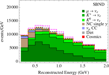
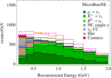
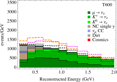
Figure 10: $\nu_{e}$ appearance spectrum at SBN detectors: (top) LAr1-ND, (middle) MicroBooNE, and (bottom) ICARUS-T600. Full data set at these three detectors are assumed (see text). The shaded histograms are the different background components as indicated in the legend (taken from Ref. Antonello et al. (2015)). Black, green, magenta and orange lines are for points 1, 2, 3 in Table 1 and the best-fit 3+1 sterile neutrino model, respectively.

III.3 Summary of oscillation constraints and sensitivities

To summarize the phenomenology of the model, we illustrate present constraints and future sensitivities on LED+ in Fig. 11. For given values of $R$, the lightest active neutrino masses $m_{0}$ and, as an example, a fixed set of $\lambda^{i}=(0.42,\,2.4,\,1.7)$ we calculate the values of $c_{i}$ in order to obtain the solar and atmospheric squared mass splittings. To perform this calculation we approximated the active neutrino masses using perturbation theory and Eqs. (7) and (13). We present the estimated allowed region at $2\sigma$ level to the left of the corresponding line by the MINOS experiment (gray solid line) and 5% deviation from the ratio of the observed event numbers to the SM prediction at reactor short baseline experiments (grey dashed line) in the plane $R-m_{0}$; as well as the projected $2\sigma$ sensitivities for the DUNE experiment (red dashed line) and for the Short-Baseline Program at Fermilab (blue line). For the latter, we used only the appearance channel. As a reference, our benchmark point 3 is shown with the red dot. We also indicate the region in which the active-sterile mixing is large (light gray shaded), parametrized by $\sum_{i}(1-|W_{i}^{00}|^{2})\geq 0.3$; as well as the region in which our approximation for the evaluation of the solar and atmospheric mass splittings is not valid (dark gray shaded region). Fig. 11 highlights the potential of the near future neutrino Fermilab program in probing LED+ models.

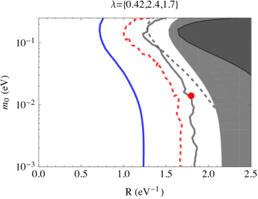
Figure 11: Present and future constraints, in the plane $R\times m_{0}$, by MINOS (gray solid line), reactor short baseline experiments (gray dashed line; 5% flux uncertainty is assumed), DUNE (red dashed line) and for the Short-Baseline Program at Fermilab (blue line; appearance mode only). For reference, the light gray shaded region indicates large active-sterile mixing, namely $\sum_{i}(1-|W_{i}^{00}|^{2})=0.3$. In the dark gray shaded region the approximation used to obtain $\Delta m^{2}_{21}$ and $\Delta m^{2}_{31}$ fails.

III.4 Kinematic Constraints

The limit on the effective electron neutrino mass from the Mainz experiment on Tritium decay is given by Kraus et al. (2013),

$$m_{\beta}\equiv\sqrt{\sum_{i=1}^{3}|U_{ei}|^{2}m_{i}^{2}}<2.3\,\mathrm{eV},$$ (20)

for three active neutrinos. This bound comes from the analysis of the last $70\,\mathrm{eV}$ below the endpoint energy $Q=18.572$ keV of the Tritium $\beta$ spectrum. In our case, since we have KK modes heavier than $1\,\mathrm{eV}$, the above approximation fails (see e.g. Ref. Esmaili and Peres (2012)) and the electron $\beta$ decay spectrum needs to be calculated exactly. This spectrum is given by

$$\beta(K_{e},Q,|U_{ei}|,|m_{\nu}|) =N_{s}F(Z,K_{e})E_{e}p_{e}\times$$ (21)

$$\times\sum_{i,j}P_{i}\xi_{i}|U_{ej}|^{2}\sqrt{\xi_{i}^{2}-m_{j}^{2}}\,\mathcal{\theta}(\xi_{i}-m_{j})$$

where $K_{e},p_{e}$ and $E_{e}$ are the electron kinetic energy, momentum and total energy, respectively. $F(Z,K_{e})$ is the Fermi function and we will approximate it as a constant for a non-relativistic electron Simpson (1981). The energy window $\xi$ is defined as $\xi_{i}=Q-w_{i}-K_{e}$, where $w_{i}$ and $P_{i}$ are the excitation energy and transition probability for the excited state $i$ of the daughter nucleus, respectively. The detailed evaluation of the electron spectrum is given in Appendix C.

To estimate the sensitivity of the Mainz experiment to our model, we define the deviation from the standard 3-neutrino predicted rate of events $S_{SM}$, for normal ordering and massless $\nu_{1}$, as

$$\delta R=1-\frac{S}{S_{SM}},$$ (22)

where $S$ is the rate of events in our model. The results are presented in Table 3. For comparison, we also show $\delta R$ for a 3+1 sterile neutrino model with $\Delta m^{2}_{e4}=10.2\,\mathrm{eV}^{2}$ and mixing angle $\sin^{2}\theta_{e4}=0.50$ (labelled Sterile I), which is marginally constrained by the Mainz experiment Kraus et al. (2013). As follows from Table 3, the three data points in our model are less constrained than Sterile I data point. Compared to point 1 and point 3, point 2 predicts smaller deviation from the Standard 3-active neutrino model prediction, due to their lighter KK modes and smaller active neutrino mixing with KK modes.

	Sterile I	Sterile II	$P_{1}$	$P_{2}$	$P_{3}$
$10^{5}\times\delta R$	156	1.40	80.8	19.3	118

Table 3: Deviation $\delta R$ from the standard 3-neutrino predicted rate of events for normal ordering and massless $\nu_{1}$, for the three benchmark points and for two reference points in a $3+1$ sterile neutrino model. Sterile I, with $\Delta m^{2}_{41}=10.2\,\mathrm{eV}^{2}$ and $\sin^{2}\theta_{e4}=0.50$, is constrained by the Mainz experiment, while Sterile II, with $\Delta m^{2}_{41}=10.2\,\mathrm{eV}^{2}$ and $\sin^{2}\theta_{e4}=0.0045$, will be constrained by KATRIN.

The future KArlsruhe TRItium Neutrino (KATRIN) experiment Angrik et al. (2005) will significantly improve the Mainz experiment bounds. For instance, it can probe a $3+1$ sterile neutrino model with $\Delta m^{2}_{41}=10.2\,\mathrm{eV}^{2}$ and the mixing angle $\sin^{2}\theta_{e4}=0.0045$ Esmaili and Peres (2012). We also include this reference point (Sterile II) in Table 3. We expect that KATRIN will be able to test the three benchmark points in our model and probe a significant region of the LED+ parameter space. It would be also interesting to study the effect of LED+ on the shape of beta spectrum which is discussed for LED model in Rodejohann and Zhang (2014) if KATRIN would cover the entire beta spectrum Mertens (2015). We leave this to a future work.

IV Other constraints

IV.1 Constraints from Higgs decay

The decay of the Higgs boson $h$ into a single KK mode is suppressed by the effective Yukawa coupling. However the total width is enhanced by summing over all KK modes, where the approximate number of modes, e.g. in a single extra dimension model, is given by $N\sim M_{h}R$. We calculate the $h$ decay width to all possible KK modes in the following. Neglecting the kinematic factor, the partial decay width to KK modes coming from $d$ extra dimensions is

$$\Gamma_{h} \sim\sum_{i=1}^{3}\sum^{m_{n}^{i}<M_{h}}_{n=0}\frac{M_{h}}{16\pi}(Y_{n}^{i})^{2}$$ (23)

$$\sim\frac{M_{h}}{8\pi}\sum_{i=1}^{3}\frac{\lambda^{2}_{i}}{M^{d}_{5}V_{d}}\prod_{k=1}^{d}(M_{h}R_{k})$$ (24)

$$\sim\frac{M_{h}}{8\pi}\sum_{i=1}^{3}\lambda^{2}_{i}\left(\frac{M_{h}}{\pi M_{5}}\right)^{d}$$ (25)

where $V_{d}$ is their volume. For $d=2$, $M_{5}=10^{6}~{}\mathrm{GeV}$, and $\lambda_{i}\sim\mathcal{O}(1)$ we obtain $\Gamma(h\to{\rm KK~{}modes)}\sim 10^{-7}~{}\mathrm{MeV}$. Therefore the $h$ decay width to KK neutrinos will not put any bound in LED+.

IV.2 Constraints from nucleosynthesis and supernova

The presence of light KK modes can have an important impact on cosmological observations. For instance, nucleosynthesis data prefer the number of fully thermalized light species to be $N_{\rm{eff}}<4$ even after doubling the systematic uncertainties Abazajian et al. (2012). In Ref. Barbieri et al. (2000), for LED without bulk masses and in the approximation of no matter asymmetry, it is shown none of the KK neutrinos are in thermal equilibrium with the plasma at MeV temperatures. The reason is that the matter effect induced by the plasma suppresses the mixing angles which are already small. In LED+ models, these mixings are even smaller for the light KK modes, which may help evade nucleosynthesis bounds. Summing over the energy density stored in all of these out-of-equilibrium KK neutrinos has large uncertainties and more work needs to be done to conclude whether BBN data will constrain the parameter space of LED+ with interesting neutrino phenomenology.

In addition to cosmological bounds, astrophysical processes may be affected by the presence of light sterile neutrinos. One well known example is supernova explosion. In particular, SN1987a Hirata et al. (1987) is likely to put constraints on $R$ since KK modes may carry away too much energy in the invisible channels from the supernova, thus modifying its evolution Barbieri et al. (2000). However, non-linear effects like collective neutrino oscillations Cacciapaglia et al. (2003) are still not well understood, and thus no robust bound can be derived on LED+ from these considerations.

V Conclusions

In this article we have studied the properties of sterile neutrinos propagating in large extra dimensions with a bulk mass term of the order of $1/R$. By adding bulk masses to the standard LED scenario, the pattern of KK sterile neutrino masses and mixings can be significantly distorted. While in LED models the first KK mode dominates the oscillation phenomenology, and one can approximate the LED model by a specific 3+1 scenario, in LED+ models the mixings with the first KK modes can be suppressed by the bulk mass terms. This increases the relative importance of the higher KK modes and leads to distinct oscillation signatures. In LED+, the correspondence with a 3+1 scenario is lost: a large number of KK modes needs to be considered in order to obtain a reasonable approximation of the oscillation probability.

We have shown that the LED+ framework provides a well defined and testable scenario that has relevant implications for neutrino oscillation experiments. It has the potential to address the observed anomalies in short baseline neutrino experiments, namely the LSND/MiniBooNE anomalous $\nu_{\mu}\to\nu_{e}$ appearance spectra, as well as the reactor and Gallium $\nu_{e}$ disappearance anomalies. We expect that the LED+ framework will be tested at the Short-Baseline Neutrino Program at Fermilab, and may also have an impact on the DUNE experiment, that may then provide additional evidence for such scenario. Moreover, the KATRIN experiment will be able to probe a significant region of the LED+ parameter space.

VI Acknowledgments

We would like Thomas Carroll, Pilar Coloma, André de Gouvêa, Enrique Fernandez-Martinez, Ornella Palamara, Zarko Pavlovic, Simon de Rijck and Zahra Tabrizi for useful discussions. This manuscript has been authored by Fermi Research Alliance, LLC under Contract No. DE-AC02-07CH11359 with the U.S. Department of Energy, Office of Science, Office of High Energy Physics. The United States Government retains and the publisher, by accepting the article for publication, acknowledges that the United States Government retains a non-exclusive, paid-up, irrevocable, world-wide license to publish or reproduce the published form of this manuscript, or allow others to do so, for United States Government purposes.

Work at University of Chicago is supported in part by U.S. Department of Energy grant number DE-FG02-13ER41958. Work at ANL is supported in part by the U.S. Department of Energy under Contract No. DE-AC02-06CH11357. C.S.M. is supported by the São Paulo Research Foundation (FAPESP) under grant 2012/21627-9 and acknowledges the hospitality and support of the Fermilab theory group. YYL is supported by the Hong Kong PhD Fellowship Scheme (HKPFS) and the Overseas Research Awards from Hong Kong University of Science and Technology. YYL would like to thank the hospitality of Enrico Fermi Institute, the University of Chicago and Fermilab where most of the work was done. This project has also received partial funding from the European Union’s Horizon 2020 research and innovation programme under the Marie Sklodowska-Curie grant agreement No 674896 and No 690575. The work of M.C. and C.W. was partially performed at the Aspen Center for Physics, which is supported by National Science Foundation grant PHY-1607611.

Appendix A Fermions in the Linear Dilaton metric

The Linear Dilaton (LD) metric is given by,

$$ds^{2}=e^{\frac{2k|z|}{3}}(\eta_{\mu\nu}dx^{\mu}dx^{\nu}-dz^{2}),$$ (26)

where we use the mostly-plus convention for the flat metric $\eta_{\mu\nu}$ and we assume $k>0$ (as argued in Ref. Giudice and McCullough (2017), negative $k$ are equivalent to positive $k$ by coordinate transformations).

The dimensional deconstruction of the 5D model (with a bulk mass term) based on this metric leads to the “clockwork mechanism” Giudice and McCullough (2017); Kaplan and Rattazzi (2016) which was explored in several applications e.g. Hambye et al. (2016); Farina et al. (2017); Kehagias and Riotto (2017). In the following, we are going to show that from the 5D perspective, fermions in the LD metric with a bulk mass can be put in equivalence with fermions in the LED with a bulk mass (see also Hambye et al. (2016)). The IR brane containing the SM fields is put at $z_{0}=0$ and the UV brane at $z_{f}=\pi R$. The 4D Planck scale $M_{\text{Pl}}$ is related to the 5D Planck scale $M_{5}$ by the following equation:

$$M^{2}_{\text{Pl}}=2\int_{0}^{\pi R}dz\,e^{kz}M_{5}^{3}=\frac{2M_{5}^{3}}{k}(e^{k\pi R}-1).$$ (27)

Notice that the relation between $M_{\text{Pl}}$ and $M_{5}$ in LD is not equivalent to LED, see Eq. (9). Let us consider a fermion $\psi$ with a bulk mass term $M(z)$,

$$S_{f}=\int d^{4}x\,dz\,\sqrt{g}\left[e_{A}^{M}i\bar{\Psi}_{0}\Gamma^{A}\overset{\leftrightarrow}{\partial_{M}}\Psi_{0}-M(z)\bar{\Psi}_{0}\Psi_{0}\right],$$ (28)

with the vierbein $e_{A}^{M}=e^{-\frac{1}{3}kz}\delta_{A}^{M}$ and $\Gamma^{A}=(\gamma^{\mu},i\gamma^{5})$. The spin connection has been dropped since its contribution cancels in our case Csaki et al. (2007). To satisfy the $S^{1}/Z_{2}$ symmetry, $M(z)$ must be odd under reflection: $M(z)=-M(-z)$. In addition, to canonically normalize the kinetic term, we use the field redefinition

$$\Psi_{0}=e^{-\frac{2kz}{3}}\Psi.$$ (29)

The action is then written as,

$$S_{f}=\!\int\!\!d^{4}x\!\!\int^{\pi R}_{0}\!\!dz\left[i\bar{\Psi}\gamma^{\mu}\overset{\leftrightarrow}{\partial_{\mu}}\Psi-\bar{\Psi}\gamma_{5}\overset{\leftrightarrow}{\partial_{z}}\Psi-e^{\frac{kz}{3}}M(z)\bar{\Psi}\Psi\right].$$ (30)

If $M(z)=0$, the KK spectrum and wave functions are the same as those in LED without bulk mass. For the zero mode, this wavefunction is flat. In the LD metric we can see that the curvature does not help to localize this mode.

If we assume a non-zero bulk mass $M(z)$ for the LED or LD metrics, we can get that the zero mode is non-flat in both cases. In particular, if we identify $M(z)e^{\frac{kz}{3}}$ in Eq. (30) with $c$ in Eq. (1), we can conclude the equivalence between LED+ and LD with a corresponding bulk mass. In the case of gravitons it is possible to show that in the curvature in LD works as a mass term Antoniadis et al. (2012) which reinforces the particular behavior of this metric. As a final comment, by having a small value for $k$ (about eV scale), one could obtain $M_{5}=10^{6}$ GeV for $R\sim\mathcal{O}(1/{\rm eV})$. This small $k$ is not unnatural as it is protected by the dilaton shift symmetry Giudice and McCullough (2017).

Appendix B Minimal flavor violation realization

In order to reduce the number of free parameters in our model and simplify the analysis, we assume a minimal flavor realization of the Yukawas and bulk mass terms as follows. In the flavor basis, Eq. (1) and the Yukawa terms in Eq. (8) are written as

$$S_{f} =\int d^{4}x\,dz\,\left[i\bar{\Psi}_{\alpha}\Gamma^{A}\overset{\leftrightarrow}{\partial_{A}}\Psi_{\alpha}-\mathcal{C}_{\alpha\beta}\bar{\Psi}_{\alpha}\Psi_{\beta}\right],$$

$$S_{Y} =-\int d^{4}x\sum_{i=1}^{3}\left(\frac{\mathcal{Y}_{\alpha\beta}}{\sqrt{M_{5}}}\bar{L}_{\alpha}\tilde{H}\Psi^{R}_{\beta}(x^{\mu},0)+h.c.\right).$$ (31)

To have both $\mathcal{C}_{\alpha\beta}$ and $\mathcal{Y}_{\alpha\beta}$ diagonalized simultaneously in the “intermediate basis” by the rotation in Eq. (10), we consider $\mathcal{C}_{\alpha\beta}$ to be a polynomial of $\mathcal{Y}^{\dagger}\mathcal{Y}$,

$$\mathcal{C}_{\alpha\beta}=\left[\sum_{a}\mathcal{M}_{a}(\mathcal{Y}^{\dagger}\mathcal{Y})^{a}\right]_{\alpha\beta},$$ (32)

where $\mathcal{M}_{a}$ are dimensionful coefficients. Then we have

$$c_{i}=\sum_{a}\mathcal{M}_{a}(\lambda^{2}_{i})^{a}.$$ (33)

Different values of $\mathcal{M}_{a}$ were chosen to get the parameters we used in our simulation. For example, we have set

$$\mathcal{M}_{0}=-0.44~{}\mathrm{eV},~{}~{}\mathcal{M}_{1}=3.9~{}\mathrm{eV},$$

$$\mathcal{M}_{2}=-2.6~{}\mathrm{eV},\mathcal{M}_{a>2}=0~{}\mathrm{eV}$$ (34)

to get the bulk mass values used for point 2. Without loss of generality we have neglected higher order contributions to $c_{i}$.

Appendix C Details for kinematic constraints

We present here some details of the beta decay rate calculation used in Section III.4. Using Eq. (21), the rate $S$ of the electrons passing the potential barrier $Uq$ and arriving at the detector is given by

$$S=\int_{0}^{\infty}\beta(K_{e},Q,|U_{ei}|,|m_{\nu}|)T(K_{e},qU)dK_{e},$$ (35)

where $T(K_{e},qU)$ is the transmission function. We use the following approximation to get a conservative estimate of $S$,

$$T(K_{e},qU)=\begin{cases}1~{}~{}~{}{\rm if}~{}~{}~{}K_{e}>qU\\ 0~{}~{}~{}{\rm if}~{}~{}~{}K_{e}<qU\end{cases}\,.$$ (36)

In addition, we approximate $\beta(K_{e},Q,|U_{ei}|,|m_{\nu}|)$ as follows:

$$\beta(K_{e},Q, |U_{ei}|,|m_{\nu}|)\simeq C\sqrt{(Q-\xi)}\xi\times$$ (37)

$$\times\sum_{j=1}^{3}\sum_{n=0}^{\infty}|U_{ej}|^{2}|W^{0n}_{j}|^{2}\sqrt{\xi^{2}-m_{j,n}^{2}}\,\theta(\xi-m_{j,n}),$$

where we assumed that the daughter nucleus is in the ground state with $\xi=Q-K_{e}$ and we used the non-relativistic relation for electron momentum, $p_{e}\simeq\sqrt{2m_{e}K_{e}}$ ($m_{e}$ is the electron mass). $C\simeq N_{s}F(Z,K_{e})E_{e}\sqrt{2m_{e}}$ is approximately a constant. We obtain the expected event rate $S$ by integrating over $1\,\mathrm{eV}<\xi<70\,\mathrm{eV}$, which is equivalent to set the potential barrier $qU=Q-70~{}\mathrm{eV}$.

References

- Pontecorvo (1957) B. Pontecorvo, Sov. Phys. JETP 6, 429 (1957), [Zh. Eksp. Teor. Fiz.33,549(1957)].
- Maki et al. (1962) Z. Maki, M. Nakagawa, and S. Sakata, Prog. Theor. Phys. 28, 870 (1962).
- Athanassopoulos et al. (1995) C. Athanassopoulos et al. (LSND), Phys. Rev. Lett. 75, 2650 (1995), eprint nucl-ex/9504002.
- Athanassopoulos et al. (1996) C. Athanassopoulos et al. (LSND), Phys. Rev. Lett. 77, 3082 (1996), eprint nucl-ex/9605003.
- Athanassopoulos et al. (1998a) C. Athanassopoulos et al. (LSND), Phys. Rev. Lett. 81, 1774 (1998a), eprint nucl-ex/9709006.
- Athanassopoulos et al. (1998b) C. Athanassopoulos et al. (LSND), Phys. Rev. C58, 2489 (1998b), eprint nucl-ex/9706006.
- Aguilar-Arevalo et al. (2001) A. Aguilar-Arevalo et al. (LSND), Phys. Rev. D64, 112007 (2001), eprint hep-ex/0104049.
- Aguilar-Arevalo et al. (2012) A. A. Aguilar-Arevalo et al. (MiniBooNE) (2012), eprint 1207.4809, URL http://lss.fnal.gov/archive/2012/pub/fermilab-pub-12-394-ad-ppd.pdf.
- Aguilar-Arevalo et al. (2013) A. A. Aguilar-Arevalo et al. (MiniBooNE), Phys. Rev. Lett. 110, 161801 (2013), eprint 1303.2588.
- Mention et al. (2011) G. Mention, M. Fechner, T. Lasserre, T. A. Mueller, D. Lhuillier, M. Cribier, and A. Letourneau, Phys. Rev. D83, 073006 (2011), eprint 1101.2755.
- Huber (2011) P. Huber, Phys. Rev. C84, 024617 (2011), [Erratum: Phys. Rev.C85,029901(2012)], eprint 1106.0687.
- An et al. (2017) F. P. An et al. (Daya Bay), Submitted to: Phys. Rev. Lett. (2017), eprint 1704.01082.
- Bahcall et al. (1995) J. N. Bahcall, P. I. Krastev, and E. Lisi, Phys. Lett. B348, 121 (1995), eprint hep-ph/9411414.
- Giunti and Laveder (2011) C. Giunti and M. Laveder, Phys. Rev. C83, 065504 (2011), eprint 1006.3244.
- Anselmann et al. (1995) P. Anselmann et al. (GALLEX), Phys. Lett. B342, 440 (1995).
- Arkani-Hamed et al. (2001) N. Arkani-Hamed, S. Dimopoulos, G. R. Dvali, and J. March-Russell, Phys. Rev. D65, 024032 (2001), eprint hep-ph/9811448.
- Dienes et al. (1999) K. R. Dienes, E. Dudas, and T. Gherghetta, Nucl. Phys. B557, 25 (1999), eprint hep-ph/9811428.
- Dienes and Sarcevic (2001) K. R. Dienes and I. Sarcevic, Phys. Lett. B500, 133 (2001), eprint hep-ph/0008144.
- Dvali and Smirnov (1999) G. R. Dvali and A. Yu. Smirnov, Nucl. Phys. B563, 63 (1999), eprint hep-ph/9904211.
- Barbieri et al. (2000) R. Barbieri, P. Creminelli, and A. Strumia, Nucl. Phys. B585, 28 (2000), eprint hep-ph/0002199.
- Davoudiasl et al. (2002) H. Davoudiasl, P. Langacker, and M. Perelstein, Phys. Rev. D65, 105015 (2002), eprint hep-ph/0201128.
- Machado et al. (2011) P. A. N. Machado, H. Nunokawa, and R. Zukanovich Funchal, Phys. Rev. D84, 013003 (2011), eprint 1101.0003.
- Berryman et al. (2016) J. M. Berryman, A. de Gouv a, K. J. Kelly, O. L. G. Peres, and Z. Tabrizi, Phys. Rev. D94, 033006 (2016), eprint 1603.00018.
- Cao et al. (2004) Q.-H. Cao, S. Gopalakrishna, and C. P. Yuan, Phys. Rev. D69, 115003 (2004), eprint hep-ph/0312339.
- Mohapatra and Perez-Lorenzana (2001) R. N. Mohapatra and A. Perez-Lorenzana, Nucl. Phys. B593, 451 (2001), eprint hep-ph/0006278.
- Diego and Quiros (2008) D. Diego and M. Quiros, Nucl. Phys. B805, 148 (2008), eprint 0804.2838.
- Lukas et al. (2000) A. Lukas, P. Ramond, A. Romanino, and G. G. Ross, Phys. Lett. B495, 136 (2000), eprint hep-ph/0008049.
- Agashe and Wu (2001) K. Agashe and G.-H. Wu, Phys. Lett. B498, 230 (2001), eprint hep-ph/0010117.
- Caldwell et al. (2001) D. O. Caldwell, R. N. Mohapatra, and S. J. Yellin, Phys. Rev. D64, 073001 (2001), eprint hep-ph/0102279.
- Lam (2002) C. S. Lam, Phys. Rev. D65, 053009 (2002), eprint hep-ph/0110142.
- Hambye et al. (2016) T. Hambye, D. Teresi, and M. H. G. Tytgat (2016), eprint 1612.06411.
- Antonello et al. (2015) M. Antonello et al. (LAr1-ND, ICARUS-WA104, MicroBooNE) (2015), eprint 1503.01520.
- Angrik et al. (2005) J. Angrik et al. (KATRIN) (2005).
- Ponton (2013) E. Ponton, in The Dark Secrets of the Terascale: Proceedings, TASI 2011, Boulder, Colorado, USA, Jun 6 - Jul 11, 2011 (2013), pp. 283–374, eprint 1207.3827, URL https://inspirehep.net/record/1122856/files/arXiv:1207.3827.pdf.
- Grossman and Neubert (2000) Y. Grossman and M. Neubert, Phys. Lett. B474, 361 (2000), eprint hep-ph/9912408.
- Parke and Ross-Lonergan (2016) S. Parke and M. Ross-Lonergan, Phys. Rev. D93, 113009 (2016), eprint 1508.05095.
- Machado et al. (2012) P. A. N. Machado, H. Nunokawa, F. A. P. dos Santos, and R. Z. Funchal, Phys. Rev. D85, 073012 (2012), eprint 1107.2400.
- Basto-Gonzalez et al. (2013) V. S. Basto-Gonzalez, A. Esmaili, and O. L. G. Peres, Phys. Lett. B718, 1020 (2013), eprint 1205.6212.
- Adamson et al. (2016) P. Adamson et al. (MINOS), Phys. Rev. D94, 111101 (2016), eprint 1608.06964.
- Bhattacharya et al. (2012) B. Bhattacharya, A. M. Thalapillil, and C. E. M. Wagner, Phys. Rev. D85, 073004 (2012), eprint 1111.4225.
- Nunokawa et al. (2005) H. Nunokawa, S. J. Parke, and R. Zukanovich Funchal, Phys. Rev. D72, 013009 (2005), eprint hep-ph/0503283.
- Aartsen et al. (2016) M. G. Aartsen et al. (IceCube), Phys. Rev. Lett. 117, 071801 (2016), eprint 1605.01990.
- Nunokawa et al. (2003) H. Nunokawa, O. L. G. Peres, and R. Zukanovich Funchal, Phys. Lett. B562, 279 (2003), eprint hep-ph/0302039.
- (44) P. Adamson et al. (MINOS), http://www-numi.fnal.gov/PublicInfo/forscientists.html.
- (45) P. Vahle, Private communication.
- Messier (1999) M. D. Messier, Ph.D. thesis, Boston U. (1999), URL http://wwwlib.umi.com/dissertations/fullcit?p9923965.
- Paschos and Yu (2002) E. A. Paschos and J. Y. Yu, Phys. Rev. D65, 033002 (2002), eprint hep-ph/0107261.
- Ambats et al. (2004) I. Ambats et al. (NOvA) (2004), eprint hep-ex/0503053.
- Yang and Woijcicki (2004) T. Yang and S. Woijcicki (NOvA) (2004), eprint Off-Axis-Note-SIM-30.
- Giunti (2017) C. Giunti, Phys. Lett. B764, 145 (2017), eprint 1608.04096.
- Hayes and Vogel (2016) A. C. Hayes and P. Vogel, Ann. Rev. Nucl. Part. Sci. 66, 219 (2016), eprint 1605.02047.
- Hampel et al. (1998) W. Hampel et al. (GALLEX), Phys. Lett. B420, 114 (1998).
- Kaether et al. (2010) F. Kaether, W. Hampel, G. Heusser, J. Kiko, and T. Kirsten, Phys. Lett. B685, 47 (2010), eprint 1001.2731.
- Abdurashitov et al. (1999) J. N. Abdurashitov et al. (SAGE), Phys. Rev. C59, 2246 (1999), eprint hep-ph/9803418.
- Abdurashitov et al. (2006) J. N. Abdurashitov et al., Phys. Rev. C73, 045805 (2006), eprint nucl-ex/0512041.
- Bahcall (1997) J. N. Bahcall, Phys. Rev. C56, 3391 (1997), eprint hep-ph/9710491.
- Frekers et al. (2011) D. Frekers et al., Phys. Lett. B706, 134 (2011).
- Kopp et al. (2013) J. Kopp, P. A. N. Machado, M. Maltoni, and T. Schwetz, JHEP 05, 050 (2013), eprint 1303.3011.
- Athanassopoulos et al. (1997) C. Athanassopoulos et al. (LSND), Nucl. Instrum. Meth. A388, 149 (1997), eprint nucl-ex/9605002.
- Collin et al. (2016) G. H. Collin, C. A. Arg elles, J. M. Conrad, and M. H. Shaevitz, Phys. Rev. Lett. 117, 221801 (2016), eprint 1607.00011.
- Gariazzo et al. (2017) S. Gariazzo, C. Giunti, M. Laveder, and Y. F. Li (2017), eprint 1703.00860.
- De Romeri et al. (2016) V. De Romeri, E. Fernandez-Martinez, and M. Sorel, JHEP 09, 030 (2016), eprint 1607.00293.
- Alion et al. (2016) T. Alion et al. (DUNE) (2016), eprint 1606.09550.
- Kraus et al. (2013) C. Kraus, A. Singer, K. Valerius, and C. Weinheimer, Eur. Phys. J. C73, 2323 (2013), eprint 1210.4194.
- Esmaili and Peres (2012) A. Esmaili and O. L. G. Peres, Phys. Rev. D85, 117301 (2012), eprint 1203.2632.
- Simpson (1981) J. J. Simpson, Phys. Rev. D23, 649 (1981).
- Rodejohann and Zhang (2014) W. Rodejohann and H. Zhang, Phys. Lett. B737, 81 (2014), eprint 1407.2739.
- Mertens (2015) S. Mertens (KATRIN), Phys. Procedia 61, 267 (2015).
- Abazajian et al. (2012) K. N. Abazajian et al. (2012), eprint 1204.5379.
- Hirata et al. (1987) K. Hirata et al. (Kamiokande-II), Phys. Rev. Lett. 58, 1490 (1987), [,727(1987)].
- Cacciapaglia et al. (2003) G. Cacciapaglia, M. Cirelli, and A. Romanino, Phys. Rev. D68, 033013 (2003), eprint hep-ph/0302246.
- Giudice and McCullough (2017) G. F. Giudice and M. McCullough, JHEP 02, 036 (2017), eprint 1610.07962.
- Kaplan and Rattazzi (2016) D. E. Kaplan and R. Rattazzi, Phys. Rev. D93, 085007 (2016), eprint 1511.01827.
- Farina et al. (2017) M. Farina, D. Pappadopulo, F. Rompineve, and A. Tesi, JHEP 01, 095 (2017), eprint 1611.09855.
- Kehagias and Riotto (2017) A. Kehagias and A. Riotto, Phys. Lett. B767, 73 (2017), eprint 1611.03316.
- Csaki et al. (2007) C. Csaki, J. Hubisz, and S. J. Lee, Phys. Rev. D76, 125015 (2007), eprint 0705.3844.
- Antoniadis et al. (2012) I. Antoniadis, A. Arvanitaki, S. Dimopoulos, and A. Giveon, Phys. Rev. Lett. 108, 081602 (2012), eprint 1102.4043.