Paul Kabaila^∗ and Rheanna Mainzer^∗∗

La Trobe University

ABSTRACT

Consider panel data modelled by a linear random intercept model that includes a time-varying covariate. Suppose that we have uncertain prior information that this covariate is exogenous. We present a new confidence interval for the slope parameter that utilizes this uncertain prior information. This interval has minimum coverage probability very close to its nominal coverage. Let the scaled expected length of this new confidence interval be its expected length divided by the expected length of the confidence interval, with the same minimum coverage, constructed using the fixed effects model. This new interval has scaled expected length that (a) is substantially less than 1 when the prior information is correct, (b) has a maximum value that is not too much larger than 1 and (c) is close to 1 when the data strongly contradict the prior information. We illustrate the properties of this new interval using an airfare data set.

* Corresponding author. Department of Mathematics and Statistics, La Trobe University, Victoria 3086, Australia. e-mail: P.Kabaila@latrobe.edu.au

** Department of Mathematics and Statistics, La Trobe University, Victoria 3086, Australia. e-mail: rmmainzer@students.latrobe.edu.au

1 INTRODUCTION

We consider panel data modelled by a linear random intercept model that includes a time-varying covariate. Irrespective of whether or not this covariate is exogenous, valid inference results from the fixed effects model. However, if this covariate is exogenous then valid and more efficient inference results from the random effects model. This greater efficiency motivates the use of this model, whenever it is appropriate, for inference.

The Hausman (1978) pretest is commonly used in practice to decide whether or not subsequent inference will be based on the assumption that the time-varying covariate is exogenous. If the null hypothesis that this covariate is exogenous is accepted then the random effects model is used for subsequent inference; otherwise the fixed effects model is used (see e.g. Hastings, 2004, Papatheodorou and Lei, 2006, Choe, 2008, and Jackowicz, Kowalewski and Kozlowki, 2013.). A somewhat similar approach is to report the inference resulting from both of these models, and to state the preferred model based on the outcome of the Hausman pretest (see e.g. Smith, Smith and Verner, 2006, and Stanca, 2006). This pretest is incorporated in popular software packages such as eViews, R, SAS and Stata.

Guggenberger (2010) and Kabaila, Mainzer and Farchione (2015, 2017) show that the effect of model selection using the Hausman pretest in this way is very damaging to hypothesis tests and confidence intervals for the slope parameter. In particular, the confidence interval constructed using the model selected by the Hausman pretest has minimum coverage probability that is typically far below the nominal coverage. This is an example of a widespread problem with confidence intervals constructed after preliminary data-based model selection (see e.g. Kabaila, 2009, and Leeb and Pötscher, 2005). As in Kabaila et al (2017), throughout the present paper we carry out inference conditional on the observed values of the time-varying covariate. The very important advantages of this conditional inference are described in the introduction to Kabaila et al (2017). These advantages include the fact that this inference is valid irrespective of how the values of the covariate are generated. In the econometric literature, an early recognition of this advantage is provided by Koopmans (1937, pp 29 and 30). In the present paper, the inference of interest is a confidence interval for the slope parameter.

As insightfully pointed out by Leamer (1978, chapter 5), preliminary data-based model selection (such as a Hausman pretest) may be motivated by the desire to utilize uncertain prior information in statistical inference. He goes even further when he states, on p.123, that “The mining of data that is common among non-experimental scientists constitutes prima facie evidence of the existence of prior information”. Leamer uses a Bayesian approach to utilize uncertain prior information in statistical inference. An alternative is to use a frequentist approach to utilize the uncertain prior information. The utilization of uncertain prior information in frequentist inference has a distinguished history. Hodges and Lehmann (1952), Pratt(1961), Stein (1962), Cohen (1972), Bickel (1984), Kempthorne (1983, 1987, 1988), Casella and Hwang (1983, 1987), Goutis and Casella (1991), Tseng and Brown (1997) and Efron (2006) are included in this history, which is briefly reviewed by Kabaila (2009, Sections 8 and 9).

In the present paper we use the frequentist approach and suppose that there is, indeed, uncertain prior information that the covariate is exogenous. If this prior information was certain then we would simply use the random effects model to construct a confidence interval with desired confidence coefficient $1-\alpha$ for the slope parameter. Recall that the confidence coefficient of a confidence interval is defined to be the infimum over the parameter space of the coverage probability of this interval. However, since we assume only uncertain prior information, we seek a confidence interval with the desired confidence coefficient and an expected length that (a) is relatively small when the prior information is correct and (b) is not too large when the prior information happens to be incorrect.

We show how the uncertain prior information that the covariate is exogenous can be utilized to construct a new confidence interval for the slope parameter with the following attractive properties. This confidence interval has a confidence coefficient that is very close to the desired value $1-\alpha$. Define the scaled expected length of this new confidence interval to be the expected length of this interval divided by the expected length of the confidence interval, with the same minimum coverage, that is constructed using the fixed effects model. This new confidence interval has scaled expected length that (a) is substantially less than 1 when the prior information is correct and (b) has maximum (over the parameter space) that is not too much larger than 1. In addition, the new confidence interval reverts to the confidence interval, with confidence coefficient $1-\alpha$ and constructed using the fixed effects model, when the data strongly contradict the prior information. Unlike the endpoints of the confidence interval constructed using a model chosen by a Hausman pretest, which are discontinuous functions of the data, the endpoints of the new confidence interval are smooth functions of the data.

Consider, as an example, the airfare data set provided by Wooldridge (2013). We are interested in the regression of the response lfare, which is the logarithm of the fare, on the covariate concen, which is the market share of the largest carrier. This is panel data with the response lfare measured for each of $N=1149$ city-pair markets over $T=4$ time points. Using an analysis conditional on the observed values of this covariate, Kabaila et al (2017) found that the confidence coefficient of the confidence interval, with nominal coverage 0.95, that results from a Hausman pretest is approximately 0.19, which is much lower than the nominal coverage. This confidence interval also has a scaled expected length that exceeds 1 throughout the parameter space.

For the linear random intercept model that we consider, the coverage probabilty of the new confidence interval for the slope parameter is a function of two unknown parameters: $\delta$, which is the ratio (variance of random effect)/(variance of random error), and $\gamma$, a parameter that takes a non-zero value unless the covariate is exogenous. In other words, the covariate is exogenous when $\gamma=0$. For this airfare data, the new confidence interval, with desired confidence coefficient 0.95, is found to have confidence coefficient that is approximately 0.9493. The coverage probability, minimized over $\gamma$, of this new confidence interval for the airfare data is graphed as a function of $\delta$ in Figure 1.

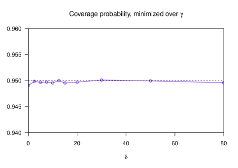
Figure 1: Graph of the coverage probability of the new confidence interval, minimized over $\gamma$, as a function of $\delta$ for the airfare data. Here $N=1149$, $T=4$ and $1-\alpha=0.95$. The confidence coefficient is estimated to be 0.9493.

Figure 2 presents graphs of the squared scaled expected length of the new confidence interval for the slope parameter, with desired confidence coefficient 0.95, as a function of $\gamma$, for $\delta\in\{1,6,12,40\}$, for the airfare data. The squared scaled expected length is directly related to the relative sample sizes required for the new confidence interval and the confidence interval, with the same confidence coefficient and constructed using the fixed effects model, to have the same expected length (cf Bickel and Doksum, 1977, p. 137). The graphs of the squared scaled expected lengths were found to be very close to being even functions of $\gamma$ and so Figure 2 presents these graphs only for $\gamma\geq 0$. How far the squared scaled expected length is below 1 when $\gamma=0$ (i.e. when the prior information that the covariate is exogenous is correct) depends on the unknown parameter $\delta$. The estimate of $\delta$ for the airfare data is 12.774, suggesting that the graph of the squared scaled expected length of the new confidence interval will be similar to the left-hand lower panel of Figure 2.

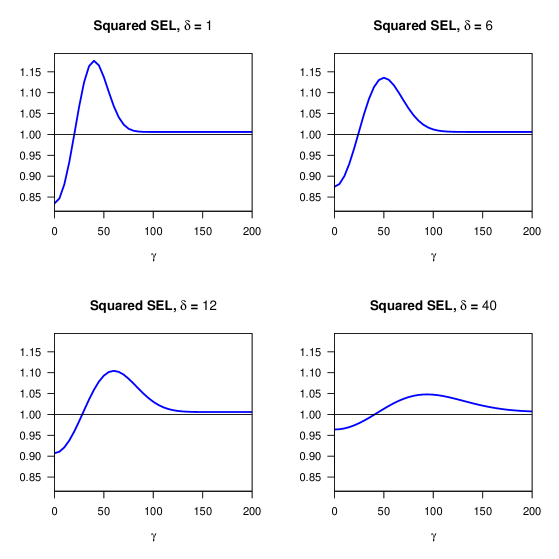
Figure 2: Graphs of the squared scaled expected length of the new confidence interval, as a function of $\gamma$ for given $\delta$ for the airfare data. Here $N=1149$, $T=4$ and $1-\alpha=0.95$.

A description of the simulation methods used to prepare Figures 1 and 2 is provided in Section 3. In the next section we describe the correlated random effects model and the new confidence interval which is obtained using the following two steps. In the first step, we suppose that $\delta$ and the random error variance are known and construct a confidence interval for the slope parameter that utilizes the uncertain prior information that the covariate is exogenous using the method of Kabaila and Giri (2009). This method has since been used in other contexts, including the construction of optimized Stein-type confidence sets for the multivariate normal mean (Abeysekera and Kabaila, 2017). In the second step, we replace these parameter values by estimates. In other words, we use the plug-in principle (Efron, 1998, Section 5).

2 THE CORRELATED RANDOM EFFECTS MODEL AND THE NEW CONFIDENCE INTERVAL

We consider a model for panel data, for which $i$ denotes the individual, household or firm etc. ($i=1,\dots,N$) and $t$ denotes time ($t=1,\dots,T$). Let $y_{it}$ and $x_{it}$ denote the response variable and the time-varying covariate, respectively, for the $i$’th individual at the $t$’th time. Our analysis is conditional on $x=(x_{11},\dots,x_{1T},\dots,x_{N1},\dots,x_{NT})$. Suppose that

$$y_{it}=a+b\,x_{it}+\xi\overline{x}_{i}+\eta_{i}+\varepsilon_{it}$$ (1)

for $i=1,\dots,N$ and $t=1,\dots,T$, where $\overline{x}_{i}=T^{-1}\sum_{t=1}^{T}x_{it}$. We assume that the $\eta_{i}$’s and the $\varepsilon_{it}$’s are independent, with the $\eta_{i}$’s independent and identically distributed (i.i.d.) $N(0,\sigma^{2}_{\eta})$ and the $\varepsilon_{it}$’s are i.i.d. $N(0,\sigma^{2}_{\varepsilon})$. Let $\delta=\sigma_{\eta}^{2}/\sigma_{\varepsilon}^{2}$. The $\varepsilon_{it}$’s and the $\eta_{i}$’s are unobserved. This is the correlated random effects model described, for example, by Wooldridge (2013, p.497). If $\xi=0$ then the $x_{it}$’s are exogenous. Thus, we call $\xi$ a non-exogeneity parameter. Our aim is to find a confidence interval for the slope parameter $b$ with the desired minimum coverage probability and expected length that (a) is relatively small when the prior information is correct and (b) is not too large when the prior information happens to be incorrect.

The new confidence interval is constructed using the following two steps. In the first step we suppose that $(\sigma_{\varepsilon},\delta)$ is known and note that, after the standard transformation described in Appendix A, the model (1) becomes a linear regression model with i.i.d. normal random errors with known variance. The method of Kabaila and Giri (2009) is then adapted to this particular case (as described in Appendix A) to find a confidence interval that has the desired coverage and expected length properties. Of course, this confidence interval is determined by $(\sigma_{\varepsilon},\delta)$. The second step is to replace the value of $(\sigma_{\varepsilon},\delta)$ used in the construction of this confidence interval by the estimator $(\widehat{\sigma}_{\varepsilon},\widehat{\delta})$ described in Subsection 2.2.

2.1 First step: confidence interval construction assuming that $\bm{(\sigma_{\varepsilon},\delta)}$ is known

The details for the first step are as follows. Suppose that $(\sigma_{\varepsilon},\delta)$ is known. Adding and subtracting $b\,\overline{x}_{i}$ to the right hand side of (1) gives

$$y_{it}=a+b_{W}(x_{it}-\overline{x}_{i})+b_{B}\,\overline{x}_{i}+\eta_{i}+\varepsilon_{it},$$ (2)

where $b_{W}=b$ and $b_{B}=b+\xi$. Let $\widehat{b}_{W}$ and $\widehat{b}_{B}$ denote the GLS estimators of $b_{W}$ and $b_{B}$, respectively, obtained using this model. Note that $\widehat{b}_{W}$ is the estimator of $b$ obtained using the fixed effects model. Now let

$$h(\sigma_{\varepsilon},\delta)=\dfrac{\widehat{b}_{W}-\widehat{b}_{B}}{\left(\text{Var}(\widehat{b}_{W}\,|\,x)+\text{Var}(\widehat{b}_{B}\,|\,x)\right)^{1/2}},$$

where $\text{Var}(\widehat{b}_{W}\,|\,x)$ and $\text{Var}(\widehat{b}_{B}\,|\,x)$ denote the variances of $\widehat{b}_{W}$ and $\widehat{b}_{B}$, respectively, conditional on $x$. Note that $h^{2}(\sigma_{\varepsilon},\delta)$ is the test statistic for a Hausman test of the null hypothesis $\xi=0$ against the alternative hypothesis $\xi\neq 0$.

Let $\text{\small SSB}=\sum_{i=1}^{N}(\overline{x}_{i}-\overline{x})^{2}$ and $\text{\small SSW}=\sum_{i=1}^{N}\sum_{j=1}^{T}(x_{it}-\overline{x}_{i})^{2}$ It follows from the proof of Lemma 1 of Kabaila et al (2017) that

$$\text{Var}(\widehat{b}_{W}\,|\,x)=\frac{\sigma^{2}_{\varepsilon}}{\text{\small SSW}}\quad\text{and}\quad\text{Var}(\widehat{b}_{B}\,|\,x)=\frac{\sigma^{2}_{\varepsilon}(\delta+T^{-1})}{\text{\small SSB}}.$$

We see from this that our assumption that $(\sigma_{\varepsilon},\delta)$ is known is needed to find $h(\sigma_{\varepsilon},\delta)$. The confidence interval for $b$, based on the fixed effects model and with coverage probability $c$, is

$$L(\sigma_{\varepsilon},c)=\left[\widehat{b}_{W}-z_{(c+1)/2}\,\left(\sigma_{\varepsilon}^{2}/\text{\small SSW}\right)^{1/2},\,\widehat{b}_{W}+z_{(c+1)/2}\,\left(\sigma_{\varepsilon}^{2}/\text{\small SSW}\right)^{1/2}\right],$$

where $z_{p}=\Phi^{-1}(p)$ and $\Phi$ denotes the $N(0,1)$ cdf.

As shown in Appendix A, after a standard transformation, the model (2) becomes a linear regression model with i.i.d. normal random errors with known variance. Let $[m\pm w]$ denote the interval $[m-w,m+w]$ ($w\geq 0$). Using the method of Kabaila and Giri (2009) as described in Appendix A, we are led to a confidence interval of the form

$$J\big{(}f_{o},f_{e};\sigma_{\varepsilon},\delta\big{)}=\left[\widehat{b}_{W}+\left(\sigma_{\varepsilon}^{2}/\text{\small SSW}\right)^{1/2}f_{o}\big{(}h(\sigma_{\varepsilon},\delta)\big{)}\pm\left(\sigma_{\varepsilon}^{2}/\text{\small SSW}\right)^{1/2}f_{e}\big{(}h(\sigma_{\varepsilon},\delta)\big{)}\right],$$

where $f_{o}:\mathbb{R}\rightarrow\mathbb{R}$ is an odd continuous function and $f_{e}:\mathbb{R}\rightarrow[0,\infty)$ is an even continuous function. Obviously, $f_{o}(0)=0$. In addition, we require that $f_{o}(x)=0$ and $f_{e}(x)=z_{1-\alpha/2}$ for $|x|\geq d$, where $d$ is a (sufficiently large) specified positive number. By construction, $J(f_{o},f_{e};\sigma_{\varepsilon},\delta)$ reverts to the confidence interval, with confidence coefficient $1-\alpha$ and constructed using the fixed effects model, when $|h|\geq d$ i.e. when the data strongly contradict the prior information. We have chosen $d=6$ because extensive numerical experimentation shows this is sufficiently large. Let ${\cal D}$ denote the class of pairs of functions $(f_{o},f_{e})$ that satisfy these requirements.

Let ${\cal C}$ denote the subset of ${\cal D}$ such that $(f_{o},f_{e})$ is fully specified by the vectors $\big{(}f_{o}(1),f_{o}(2),\dots,f_{o}(5)\big{)}$ and $\big{(}f_{e}(0),f_{e}(1),\dots,f_{e}(5)\big{)}$ as follows. By assumption, $\big{(}f_{o}(-1),f_{o}(-2),\dots,f_{o}(-5)\big{)}=\big{(}-f_{o}(1),-f_{o}(2),\dots,-f_{o}(5)\big{)}$ and $\big{(}f_{e}(-1),\dots,f_{e}(-5)\big{)}\newline =\big{(}f_{e}(1),\dots,f_{e}(5)\big{)}$. The values of $f_{o}(x)$ and $f_{e}(x)$ for any $x\in[-6,6]$ are found by natural cubic spline interpolation for the given values of $f_{o}(j)$ and $f_{e}(j)$ for $j=-6,-5,\dots,0,1,\dots,5,6$. We will numerically compute $(f_{o},f_{e})\in{\cal C}$ such that $J\big{(}f_{o},f_{e};\sigma_{\varepsilon},\delta\big{)}$ has minimum coverage probability $1-\alpha$ and scaled expected length that (a) is substantially less than 1 when the prior information is correct and (b) has maximum (over the parameter space) that is not too much larger than 1.

We now describe the numerical constrained optimization method used to find the pair of functions $(f_{o},f_{e})\in{\cal C}$ satisfying these conditions. Let $\gamma=\xi\,N^{1/2}/\sigma_{\varepsilon}$, a scaled version of the non-exogeneity parameter $\xi$. By Theorem B.1, stated in Appendix B, for any given $(f_{o},f_{e})\in{\cal D}$, the conditional coverage probability $P\big{(}b\in J(f_{o},f_{e};\sigma_{\varepsilon},\delta)\,\big{|}\,x\big{)}$ is a function of $(\gamma,\delta$). We therefore denote this coverage probability by $CP(\gamma,\delta;f_{o},f_{e})$. We define the conditional scaled expected length of $J(f_{o},f_{e};\sigma_{\varepsilon},\delta)$ as

$$\frac{E\big{(}\text{length of}\ J(f_{o},f_{e};\sigma_{\varepsilon},\delta)\,\big{|}\,x\big{)}}{\text{length of}\ L(\sigma_{\varepsilon},1-\alpha)}.$$

By Theorem B.1, stated in Appendix B, for any given $(f_{o},f_{e})\in{\cal D}$, this scaled expected length is a function of $(\gamma,\delta$). We therefore denote this scaled expected length by $SEL(\gamma,\delta;f_{o},f_{e})$.

Suppose for the moment that $\varphi$, satisfying $0\leq\varphi\leq 1$, is given. Numerically compute the pair of functions $(f_{o},f_{e})\in{\cal C}$ that minimizes the objective function

$$(1-\varphi)\big{(}SEL(\gamma=0,\delta;f_{o},f_{e})-1\big{)}+\varphi\int_{-\infty}^{\infty}\big{(}SEL(\gamma,\delta;f_{o},f_{e})-1\big{)}\,d\gamma,$$ (3)

subject to the inequality constraint that $CP(\gamma,\delta;f_{o},f_{e})\geq 1-\alpha$ for all $\gamma\in\mathbb{R}$. This numerical constrained optimization is made feasible by the computationally convenient expressions for $CP(\gamma,\delta;f_{o},f_{e})$, which is an even function of $\gamma$, and the objective function (3) given in Appendix A. For the computations, the coverage inequality constraint $CP(\gamma,\delta;f_{o},f_{e})\geq 1-\alpha$ for all $\gamma\geq 0$ is replaced by $CP(\gamma,\delta;f_{o},f_{e})\geq 1-\alpha$ for a well chosen finite set of nonnegative values of $\gamma$. Let $\big{(}f_{o}^{*}(\,\cdot\,;\delta,\varphi),f_{e}^{*}(\,\cdot\,;\delta,\varphi)\big{)}$ denote the value of $(f_{o},f_{e})\in{\cal C}$ that results from this numerical computation.

For $\varphi=1$ this numerical computation recovers the confidence interval $L(\sigma_{\varepsilon},1-\alpha)$ for $b$, based on the fixed effects model and with coverage probability $1-\alpha$. As $\varphi$ decreases from this value, this computation puts increasing weight on achieving a small value of $SEL(\gamma=0,\delta;f_{o},f_{e})$, which results in a smaller value of $SEL\big{(}\gamma=0,\delta;f_{o}^{*}(\,\cdot\,;\delta,\varphi),f_{e}^{*}(\,\cdot\,;\delta,\varphi)\big{)}$ i.e. an improved confidence interval performance when the prior information that $\gamma=0$ is correct. However, as $\varphi$ decreases

$$\max_{\gamma}SEL\big{(}\gamma,\delta;f_{o}^{*}(\,\cdot\,;\delta,\varphi),f_{e}^{*}(\,\cdot\,;\delta,\varphi)\big{)}$$

increases i.e. the performance of the confidence interval when the prior information happens to be incorrect is degraded. Numerical experimentation revealed that a reasonable tradeoff between this improvement and degradation in performance resulted when $\varphi$ was chosen such that the “gain” when the prior information is correct, as measured by

$$1-\bigg{(}SEL\big{(}\gamma=0,\delta;f_{o}^{*}(\,\cdot\,;\delta,\varphi),f_{e}^{*}(\,\cdot\,;\delta,\varphi)\big{)}\bigg{)}^{2},$$ (4)

is equal to the maximum possible “loss” when the prior information happens to be incorrect, as measured by

$$\left(\max_{\gamma}SEL\big{(}\gamma,\delta;f_{o}^{*}(\,\cdot\,;\delta,\varphi),f_{e}^{*}(\,\cdot\,;\delta,\varphi)\big{)}\right)^{2}-1.$$ (5)

Clearly, the value of $\varphi$ chosen in this way is determined by $\delta$ (assuming that $x$ is given) and so we denote it by $\varphi^{*}(\delta)$. In other words, the confidence interval constructed assuming that $(\sigma_{\varepsilon},\delta)$ is known is

$$CI(\sigma_{\varepsilon},\delta)=J\Big{(}f_{o}^{*}(\,\cdot\,;\delta,\varphi^{*}(\delta)),\,f_{e}^{*}(\,\cdot\,;\delta,\varphi^{*}(\delta));\,\sigma_{\varepsilon},\,\delta\Big{)}.$$

For $\delta\in\{1,6,12,40\}$, Figure 3 presents graphs of the functions $f_{o}^{*}(\,\cdot\,;\delta,\varphi^{*}(\delta))$ (top panel) and $f_{e}^{*}(\,\cdot\,;\delta,\varphi^{*}(\delta))$ (bottom panel) for $1-\alpha=0.95$, for the airfare data. Because $f_{o}^{*}(\,\cdot\,;\delta,\varphi^{*}(\delta))$ is an odd function and $f_{e}^{*}(\,\cdot\,;\delta,\varphi^{*}(\delta))$ is an even function, we present these graphs only for $x\geq 0$.

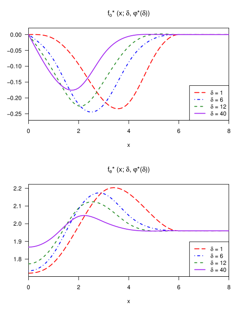
Figure 3: Graphs of the functions $f_{o}^{*}(\,\cdot\,;\delta,\varphi^{*}(\delta))$ (top panel) and $f_{e}^{*}(\,\cdot\,;\delta,\varphi^{*}(\delta))$ (bottom panel) for $1-\alpha=0.95$ and each $\delta\in\{1,6,12,40\}$, for the airfare data.

For the airfare data and $1-\alpha=0.95$, the infimum and supremum of the coverage probability of $CI(\sigma_{\varepsilon},\delta)$, conditional on $x$, are 0.9500 and 0.9507, respectively. In other words, the coverage probability of this interval, conditional on $x$, is very close to $1-\alpha=0.95$ for all $(\gamma,\delta)$. For the airfare data, Figure 4 presents graphs of the squared scaled expected length of $CI(\sigma_{\varepsilon},\delta)$ as a function of $\gamma$ for each $\delta\in\{1,6,12,40\}$ and $1-\alpha=0.95$. We can see from this figure that, for each of these values of $\delta$, the minimum squared scaled expected length is below 1 at $\gamma=0$ (i.e. when the uncertain prior information is correct), the maximum squared scaled expected length is not too much greater than 1, and the squared scaled expected length approaches 1 as $\gamma$ increases. This last property is a consequence of the fact that, by construction, $CI(\sigma_{\varepsilon},\delta)$ reverts to the confidence interval $L(\sigma_{\varepsilon},1-\alpha)$, based on the fixed effects model, when the data strongly contradict the prior information.

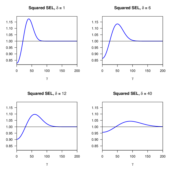
Figure 4: Graphs of the squared scaled expected length of $CI(\sigma_{\varepsilon},\delta)$ as a function of $\gamma$ for $\delta\in\{1,6,12,40\}$ and $1-\alpha=0.95$.

2.2 Second step: replace the true parameter value $\bm{(\sigma_{\varepsilon},\delta)}$ by an
estimator $\bm{(\widehat{\sigma}_{\varepsilon},\widehat{\delta})}$

We use the same estimator $(\widehat{\sigma}_{\varepsilon},\widehat{\delta})$ of $(\sigma_{\varepsilon},\delta)$ as Kabaila et al (2017). The motivation for this estimator is provided in Section 2.1 of Kabaila et al (2017). Define $\overline{y}_{i}=T^{-1}\sum_{t=1}^{T}y_{it}$ and $\overline{\varepsilon}_{i}=T^{-1}\sum_{t=1}^{T}\varepsilon_{it}$. Let $r_{it}=(y_{it}-\overline{y}_{i})-\widehat{b}_{W}(x_{it}-\overline{x}_{i})$. The estimator of $\sigma_{\varepsilon}^{2}$ that we use is

$$\widehat{\sigma}_{\varepsilon}^{2}=\dfrac{1}{N(T-1)}\sum_{i=1}^{N}\sum_{t=1}^{T}r_{it}^{2}.$$

Let $\widehat{a}$ denote the GLS estimator of $a$ based on the model (2). Define $\widetilde{r}_{i}=\overline{y}_{i}-(\widehat{a}+\widehat{b}_{B}\,\overline{x}_{i})$. The estimator of $\delta$ that we use is $\widehat{\delta}=\widehat{\sigma}_{\eta}^{2}\,/\,\widehat{\sigma}_{\varepsilon}^{2}$, where

$$\widehat{\sigma}_{\eta}^{2}=\dfrac{1}{N}\sum_{i=1}^{N}\widetilde{r}_{i}^{2}-\dfrac{\widehat{\sigma}_{\varepsilon}^{2}}{T}.$$

The second step in the construction of the new confidence interval is to replace $(\sigma_{\varepsilon},\delta)$ by the estimator $(\widehat{\sigma}_{\varepsilon},\widehat{\delta})$ in $CI(\sigma_{\varepsilon},\delta)$. In other words, we use the plug-in principle (Efron, 1998, Section 5). The resulting confidence interval is $CI(\widehat{\sigma}_{\varepsilon},\widehat{\delta})$. As proved in Appendix B, the conditional coverage probability and the scaled expected length of this confidence interval are both functions of $(\gamma,\delta)$.

As noted in Subsection 2.1, for $(\sigma_{\varepsilon},\delta)$ assumed known, the infimum over $(\gamma,\delta)$ of the coverage probability of $CI(\sigma_{\varepsilon},\delta)$, conditional on $x$, is 0.9500 (accurate to four digits after the decimal point) which is very close to $1-\alpha=0.95$. As evidenced by Figure 1, this very desirable property is, to a large extent, inherited by the new confidence interval obtained through the application of the plug-in principle. A comparison of Figures 2 and 4 shows that the squared scaled expected length of $CI(\widehat{\sigma}_{\varepsilon},\widehat{\delta})$ is very close to the squared scaled expected length of $CI(\sigma_{\varepsilon},\delta)$. To summarize, for the airfare data the plug-in principle works well.

3 SIMULATION METHODS USED TO EVALUATE THE CONDITIONAL COVERAGE AND SCALED EXPECTED LENGTH OF THE NEW CONFIDENCE INTERVAL

In this section we briefly describe the two main ideas employed in the simulation methods that are used to evaluate the conditional coverage and the scaled expected length of the new confidence interval. A detailed description of these simulation methods is given in Appendix C.

The first main idea is as follows. For each given value of $\delta$, the functions $f_{o}^{*}(\,\cdot\,;\delta,\varphi^{*}(\delta))$ and $f_{e}^{*}(\,\cdot\,;\delta,\varphi^{*}(\delta))$ are found using the method described in Subsection 2.1, with computation time of the order of 1 minute. To make the simulations computationally feasible, we precompute the functions $f_{o}^{*}\big{(}\,\cdot\,;\delta,\varphi^{*}(\delta)\big{)}$ and $f_{e}^{*}\big{(}\,\cdot\,;\delta,\varphi^{*}(\delta)\big{)}$ for a grid of 11 values of $\delta$, denoted by $\delta_{1},\dots,\delta_{11}$. For any given $\delta\in[\delta_{j},\delta_{j+1}]$ and given $x\in[-6,6]$, the value of $f_{o}^{*}\big{(}x;\delta,\varphi^{*}(\delta)\big{)}$ is obtained by linear interpolation in $\delta$ from $f_{o}^{*}\big{(}x;\delta_{j},\varphi^{*}(\delta_{j})\big{)}$ and $f_{o}^{*}\big{(}x;\delta_{j+1},\varphi^{*}(\delta_{j+1})\big{)}$.

The grid of 11 values of $\delta$ is obtained as follows. Let

$$\rho(\delta)=-\left(\dfrac{r(x)}{r(x)+\delta+T^{-1}}\right)^{1/2},$$ (6)

where $r(x)=\text{\small SSB}/\text{\small SSW}$. It can be shown that $\rho(\delta)$ is the correlation between $\widehat{b}_{W}$ and $\widehat{b}_{B}-\widehat{b}_{W}$. Because $r(x)$ and $\delta$ are nonnegative, $\rho(\delta)\in(-1,0]$. To obtain the grid of values of $\delta$ we begin with the grid $\rho_{1}=0,\rho_{2}=-0.1,\rho_{3}=-0.2,\dots,\rho_{10}=-0.9,\rho_{11}=-0.97$ of values of $\rho$. We then find $\delta_{j}$ by solving for $\delta$ in $\rho(\delta)=\rho_{j}$ ($j=1,\dots,11$). Our grid of values of $\delta$ is, then, $\delta_{1},\dots,\delta_{11}$. Note that when $\rho(\delta)=0$, $CI(\sigma_{\varepsilon},\delta)$ is equal to $L(\sigma_{\varepsilon},1-\alpha)$.

The second main idea is as follows. Define $\eta_{i}^{{\dagger}}=\eta_{i}/\sigma_{\eta}$ and $\varepsilon_{it}^{{\dagger}}=\varepsilon_{it}/\sigma_{\varepsilon}$ for $i=1,\dots,N$ and $t=1,\dots,T$. Observe that the $\eta_{i}^{{\dagger}}$’s and $\varepsilon_{it}^{{\dagger}}$’s are i.i.d. $N(0,1)$. It follows from Kabaila et al (2017, Appendix A.3) that the conditional coverage probability and scaled expected length of the new confidence interval $CI(\widehat{\sigma}_{\varepsilon},\widehat{\delta})$ can be expressed in terms of the $\eta_{i}^{{\dagger}}$’s, $\varepsilon_{it}^{{\dagger}}$’s, $\delta$, $\gamma$ and $x$. We use the $\eta_{i}^{{\dagger}}$’s and $\varepsilon_{it}^{{\dagger}}$’s to drive the simulations, thereby removing the need to specify values for either $\sigma_{\varepsilon}$ or $\sigma_{\eta}$.

4 ANALYSIS OF THE ROBUSTNESS OF THE NEW CONFIDENCE INTERVAL

The new confidence interval is constructed assuming that the $\eta_{i}$’s and the $\varepsilon_{it}$’s are independent, with the $\eta_{i}$’s i.i.d $N(0,\sigma^{2}_{\eta})$ and the $\varepsilon_{it}$’s are i.i.d. $N(0,\sigma^{2}_{\varepsilon})$. As previously, let $\varepsilon_{it}^{{\dagger}}=\varepsilon_{it}/\sigma_{\varepsilon}$ and $\eta_{i}^{{\dagger}}=\eta_{i}/\sigma_{\eta}$, so that the $\varepsilon_{it}^{{\dagger}}$’s and the $\eta_{i}^{{\dagger}}$’s are i.i.d. $N(0,1)$. It follows from Kabaila, Mainzer and Farchione (2017, Appendix A.3) that the conditional coverage probability and scaled expected length of the new confidence interval $CI(\widehat{\sigma}_{\varepsilon},\widehat{\delta})$ can be expressed in terms of the $\eta_{i}^{{\dagger}}$’s, $\varepsilon_{it}^{{\dagger}}$’s, $\delta$, $\gamma$ and $x$.

In the Supplementary Material we suppose that the $\eta_{i}^{{\dagger}}$’s and $\varepsilon_{it}^{{\dagger}}$’s are still independent, but with the $\eta_{i}^{{\dagger}}$’s identically distributed with a skewed standardized Student’s $t$-distribution and the $\varepsilon_{it}^{{\dagger}}$’s identically distributed with a, possibly different, skewed standardized Student’s $t$-distribution. For the airfare data, we assess the impact of this change of distributions on the following three properties of the new confidence interval: the minimum conditional coverage probability, the scaled expected length for $\gamma=0$ and the scaled expected length, maximized over $\gamma$. As noted earlier, this confidence interval is constructed assuming that the $\varepsilon_{it}^{{\dagger}}$’s and $\eta_{i}^{{\dagger}}$’s are i.i.d. $N(0,1)$. In other words, we assess the robustness of these properties of the new confidence interval to replacement of the distributions of the $\eta_{i}^{{\dagger}}$’s and $\varepsilon_{it}^{{\dagger}}$’s by skewed standardized Student’s $t$-distributions. As shown in the Supplementary Material, these properties are very robust to this replacement.

5 DISCUSSION

Until the present paper, the applied econometrician has been faced with choosing between the following two options. The first of these options is to carry out a Hausman pretest for exogeneity followed by the construction of the confidence interval for the slope parameter, leading to a confidence interval with unacceptably poor coverage properties. The second of these options is to always construct the confidence interval using the fixed effects model i.e. to always avoid using the Hausman pretest. Neither of these options would seem to be particularly attractive to the applied econometrician.

The new confidence interval described in the present paper provides an intermediate between these two options and, in a sense, combines the best features of both. To an excellent approximation, the new confidence interval has the desired minimum coverage probability. The test statistic for the Hausman pretest enters into the expression for the new confidence interval. Furthermore, this confidence interval reduces to the confidence interval obtained using the fixed effects model when the value of the test statistic for the Hausman pretest strongly contradicts the prior information.

We have defined the “gain” of the new confidence interval to be 1 minus its squared scaled expected length, when the prior information is correct (i.e. when the covariate is exogenous). We have also defined the maximum possible “loss” to be the maximum of the squared scaled expected length minus 1, when the prior information happens to be incorrect. For the new confidence interval, we have set the “gain” equal to the maximum possible “loss”. However, if the data strongly contradict the prior information then the “loss” is negligible.

Put another way, the new confidence interval does not dominate the confidence interval, with the same confidence coefficient, obtained using the fixed effects model. Indeed, the fact that the application of the plug-in principle works so well and the admissibility result of Kabaila, Giri and Leeb (2010, Section 4) suggest that it is impossible to find a confidence interval that dominates the confidence interval obtained using the fixed effects model. Overall, the new confidence interval should only be used when there is some reasonable confidence (although not certainty) in the prior information that the covariate is exogenous. Of course, the decision as to whether or not the new confidence interval will be used must be made prior to examination of the vector of observed responses.

The new confidence interval is constructed using the method of Kabaila and Giri (2009), as described in Appendix A. The computation of this confidence interval has previously been carried out using the numerical constrained optimization function fmincon in the MATLAB Optimization Toolbox. The MATLAB programs for the computation of this confidence interval and its conditional coverage and scaled expected length have been translated, with improvements, to R programs, which will be made available in an R package.

REFERENCES

Abeysekera, W. and P. Kabaila (2017) Optimized recentered confidence spheres for the multivariate normal mean. Electronic Journal of Statistics 11, 1798–1826.
Bickel, P.J. (1984) Parametric robustness: small biases can be worthwhile. Annals of Statistics 12, 864–879.
Bickel, P.J. and K.A. Doksum (1977) Mathematical Statistics, Basic Ideas and Selected Topics Holden-Day.
Casella, G. and J.T. Hwang (1983) Empirical Bayes confidence sets for the mean of a multivariate normal distribution. Journal of the American Statistical Association 78, 688–698.
Casella, G. and J.T. Hwang (1987) Employing vague prior information in the construction of confidence sets. Journal of Multivariate Analysis 21, 79–104.
Choe, J. (2008) Income inequality and crime in the United States. Economics Letters 101, 31–33.
Cohen, A. (1972) Improved confidence intervals for the variance of a normal distribution. Journal of the American Statistical Association 67, 382–387.
Efron, B. (1998) R.A. Fisher in the 21st century. Statistical Science 13, 95–112.
Efron, B. (2006) Minimum volume confidence regions for a multivariate normal mean vector. Journal of the Royal Statistical Society, Series B 68, 655–670.
Giri, K. (2008) Confidence Intervals in Regression Utilizing Prior Information. Unpublished PhD thesis.
Goutis, C. and G. Casella (1991) Improved invariant confidence intervals for a normal variance. Annals of Statistics 19, 2015–2031.
Guggenberger, P. (2010) The impact of a Hausman pretest on the size of a hypothesis test: the panel data case. Journal of Econometrics 156, 337–343.
Hastings, J.S. (2004) Vertical relationships and competition in retail gasoline markets: Empirical evidence from contract changes in Southern California. American Economic Review 94, 317–328.
Hausman, J. A. (1978) Specification tests in econometrics. Econometrica 46, 1251–1271.
Hodges, J.L. and E.L. Lehmann (1952) The use of previous experience in reaching statistical decisions. Annals of Mathematical Statistics 23, 396–407.
Jackowicz, K., O. Kowalewski and Ł. Kozłowski (2013) The influence of political factors on commercial banks in Central European countries. Journal of Financial Stability 9, 759–777.
Kabaila, P. (2009) The coverage properties of confidence regions after model selection. International Statistical Review 77, 405–414.
Kabaila, P. and K. Giri (2009) Confidence intervals in regression utilizing prior information. Journal of Statistical Planning and Inference 139, 3419–3429.
Kabaila, P., K. Giri and H. Leeb (2010) Admissibility of the usual confidence interval in linear regression. Electronic Journal of Statistics 4, 300–312.
Kabaila, P. and H. Leeb (2006) On the large-sample minimal coverage probability of confidence intervals after model selection. Journal of the American Statistical Association 101, 619–629.
Kabaila, P., R. Mainzer and D. Farchione (2015) The impact of a Hausman pretest, applied to panel data, on the coverage probability of confidence intervals. Economics Letters 131, 12–15.
Kabaila, P., R. Mainzer and D. Farchione (2017) Conditional assessment of the impact of a Hausman pretest on confidence intervals. Statistica Neerlandica
Kempthorne, P.J. (1983) Minimax-Bayes compromise estimators. In 1983 Business and Economic Statistics Proceedings of the American Statistical Association, pp.568–573, Washington DC.
Kempthorne, P.J. (1987) Numerical specification of discrete least favourable distributions. SIAM Journal of Scientific and Statistical Computing 8, 171–184.
Kempthorne, P.J. (1988) Controlling risks under different loss functions: the compromise decision problem. Annals of Statistics 16, 1594–1608.
Koopmans, T.C. (1937) Linear Regression Analysis of Economic Time Series. Haarlem, Netherlands: Bohn.
Leamer, E. E. (1978) Specification Searches: Ad Hoc Inference with Nonexperimental Data. New York: Wiley.
Leeb, H. and B. Pötscher (2005) Model selection and inference: facts and fiction. Econometric Theory 21, 21–59.
Papatheodorou, A. and Z. Lei (2006) Leisure travel in Europe and airline business models: A study of regional airports in Great Britain. Journal of Air Transport Management 12, 47–52.
Pratt, J.W. (1961) Length of confidence intervals. Journal of the American Statistical Association 56, 549–657.
Smith, N., V. Smith and M. Verner (2006) Do women in top management affect firm performance? A panel study of 2,500 Danish firms. International Journal of Productivity and Performance Management 55, 569–593.
Stanca, L. (2006) The effects of attendance on academic performance: panel data evidence for Introductory Microeconomics. The Journal of Economic Education 37, 251–266.
Stein, C. (1962) Confidence sets for the mean of a multivariate normal distribution. Journal of the Royal Statistical Society, Series B 9, 1135–1151.
Tseng, Y.L. and L.D. Brown (1997) Good exact confidence sets for a multivariate normal mean. Annals of Statistics 5, 2228–2258.
Wooldridge, J. M. (2013), Introductory Econometrics: a Modern Approach, 5th edtion. Ohio: South-Western.
APPENDIX A
Standard transformation of the model (2) when is assumed to be known
The covariance matrix of is , where is an block diagonal matrix with identical block diagonal elements each of which is the matrix , where is a -vector of 1’s. Also, is the block diagonal matrix with identical block diagonal elements, each of which is the matrix . Premultiplying (A.7) by gives