Influence of subgrid scale models on the buffer sublayer in channel flow

Abstract

Subgrid-scale (SGS) models are critical in large-eddy simulations (LES) of turbulent flows. In this paper we conduct a comparative study on different SGS models, including one-k-equation, wall-adapting local eddy-viscosity (WALE), Sigma and shear-constrained model. Wall-resolved LES simulations of channel flows are performed with a finite volume code at shear Reynolds number $Re_{\tau}=395$. In the simulations, the buffer sublayer turns out to be the most sensitive to the SGS model. Through the analysis of the mean velocity, the second-order moments, the SGS viscosity and the fluctuating vorticities, it is shown that the WALE and Sigma model outperform others significantly in terms of fluctuations while the constrained model improves slightly the mean velocity. The results also indicate that the SGS dissipation influences strongly the velocity fluctuations but not the mean flow nor the log-layer mismatch.

I Introduction

The governing equations for LES simulaton of incompressible turbulent flows are the filtered Navier-Stokes equations Lesieur and Métais (1996); Meneveau and Katz (2000),

$$\nabla\cdot\widetilde{\textbf{u}} =0,$$ (1a)

$$\partial_{t}\widetilde{\textbf{u}}+\widetilde{\textbf{u}}\nabla\widetilde{\textbf{u}} =-\nabla\widetilde{p}+\nu\nabla^{2}\widetilde{\textbf{u}}-\nabla\cdot\tau,$$ (1b)

where $\widetilde{p}$ and $\widetilde{\textbf{u}}$ are the filtered pressure and velocity fields, and $\tau_{ij}=\widetilde{u_{i}u_{j}}-\widetilde{u_{i}}\widetilde{u_{j}}$ is the SGS stress tensor. The tilde denotes the filter operator which will be hereafter omitted for simplicity. Modeling the SGS flow motions must be based on a functional form of $\tau$ using the filtered velocity u. This seemingly uncomplicated problem has been scrutinized for almost half century yet remains a challenge.

The first SGS model was proposed in 1960s by Smagorinsky Smagorinsky (1963) and Lilly Lilly (1967), and was inspired by the eddy-viscosity concept $\tau_{ij}=-2\nu_{SGS}S_{ij}$. Here $\nu_{SGS}=l_{S}^{2}|S|$ is the SGS viscosity, $S_{ij}=(u_{i,j}+u_{j,i})/2$ is the rate-of-strain tensor of the filtered velocity and $l_{S}=C_{S}\Delta$ denotes the Smagorinsky length scale. Even though it is affected by a consistent overprediction of velocity in the logarithmic region of boundary-layer flows (the log-layer mismatch problem), the Smagorinsky model is still widely used by CFD practitioners due to its simplicity and numerical stability. Many variants have been ever since developed to improve the Smagorinsky model. Schumann Schumann (1975) proposed a kinetic energy model where the SGS kinetic energy is solved by a transport equation and its square root is used as a velocity scale in the model. Another important development is the dynamic Smagorinsky model Germano et al. (1991), which is based on the Germano identity and the scale-invariance assumption of the model coefficient near the cut-off scale. To account for situations where the scale-invariance assumption does not hold, e.g., near-surface regions in atmospheric boundary layer flows, Porté-Agel and Meneveau Porté-Agel, Meneveau, and Parlange (2000) proposed a scale-dependent dynamic SGS model. However, the averaging procedure in dynamic models renders difficult their application in complex flows. Another group of models is based on the invariants of a symmetric tensor that depends on the gradient of the filtered velocity Trias et al. (2015). This group includes, among many others, the wall-adapting local eddy-viscosity model (WALE) Nicoud and Ducros (1999), the Vreman’s model Vreman (2004), the Verstappen’s model Verstappen (2011) and the Sigma model Nicoud et al. (2011). Similar to the Smagorinsky model, these models are local and hence are suitable for complex flows and geometries.

Another interesting idea on SGS modeling, which was also introduced by Schumann Schumann (1975), is to decompose the SGS stress into a mean and a fluctuating part following the concept of Reynolds’ decomposition. The inhomogeneous effects near the wall, which cause problems in Smagorinsky model, are thus taken into account in the mean part. Based on this idea, many SGS models have been proposed, including the two-part model by Sullivan et al. Sullivan, McWilliams, and Moeng (1994), the shear-improved model by Lévêque et al. Lévêque et al. (2007) and the recently-developed constrained SGS (CSGS) model Chen et al. (2012). The CSGS model uses the existing knowledge on the mean Reynold stress as a constraint in the SGS model and models only the fluctuation part. The knowledge of the mean quantity can be obtained from high-fidelity direct numerical simulation (DNS), experiments, analytical solutions or even low-fidelity RANS simulations. According to Chen et al. (2012), this model achieves accurate turbulent statistics while keeping the computational cost reasonable. Note that CSGS model relies heavily on the accuracy of the mean or second-moment source data, which becomes impractical for flows without reliable information on these data.

The purpose of this paper is to evaluate the performance of recently proposed SGS models and to gain insights into the SGS modeling problems by performing wall-resolved LES simulations of channel flows at a moderate Reynolds number. Four SGS models are chosen for this comparative study: one-k-equation model (kEqn), WALE, sigma, and CSGS. The details of these four SGS models are given in Section II. The simulation parameters and configurations are described in Section III. The results and their discussion are presented in Sections IV and V.

II SGS models

II.1 kEqn model

The kEqn model Yoshizawa (1985); de Villiers (2006) consists of solving a transport equation of the SGS kinetic energy

$$\partial_{t}k_{SGS}+\textbf{u}\nabla k_{SGS}=(\nu_{SGS}+\nu)\Delta k_{SGS}+2\nu_{SGS}|S|^{2}-\frac{C_{\epsilon}k_{SGS}^{3/2}}{\Delta},$$ (2)

where $C_{k}$, $C_{\epsilon}$ are constants. Typically, $C_{k}=0.094$ and $C_{\epsilon}=1.048$. The terms in the right hand side denote the viscous and turbulent diffusion, the gradient diffusion (the energy transfer between the filtered and sub-grid scales), and the dissipation, respectively. The square root of $k_{SGS}$ is taken as the velocity scale in the definition of the SGS viscosity,

$$\nu_{SGS}=C_{k}\sqrt{k_{SGS}}\Delta.$$ (3)

Compared to the Smagorinsky model Smagorinsky (1963), the kEqn model takes into account history and spatial effects. However, in practice, both models yield very close results. In the equilibrium state they are statistically equivalent.

II.2 WALE model

The WALE model was developed by Nicoud and Ducros Nicoud and Ducros (1999) in order to remedy the imperfection of the Smagorinsky model. In the Smagorinsky model, the SGS viscosity does not go to zero as the wall is approached. This causes an overestimation of the SGS dissipation and the log-layer mismatch problem. The WALE model is constructed from the invariants of the square of the velocity gradient tensor and achieves the correct scaling behavior near the wall. The WALE model preserves the property of locality, meaning that only local quantities are required to evaluate the model at any point in space and time. The model reads

$$\nu_{SGS} =(C_{w}\Delta)^{2}\mathcal{D}_{w}(\textbf{u}),$$ (4a)

$$\mathcal{D}_{w} =\frac{(S_{ij}^{d}S_{ij}^{d})^{3/2}}{(S_{ij}S_{ij})^{5/2}+(S_{ij}^{d}S_{ij}^{d})^{5/4}},$$ (4b)

where $\mathcal{D}_{w}$ is a differential operator, $S_{ij}^{d}$ is the traceless symmetric part of the square of the velocity gradient tensor, and $C_{w}\simeq 0.165$.

II.3 Sigma model

Proposed also by Nicoud et al. Nicoud et al. (2011), the Sigma model is an advanced variant of WALE, embracing a broader range of applicability. Instead of being based on the invariants of the velocity gradient functionals, the Sigma model employs the singular values of the velocity gradient tensor $\textbf{g}=u_{i,j}$. The Sigma model is

$$\nu_{SGS} =(C_{\sigma}\Delta)^{2}\mathcal{D}_{\sigma}(\textbf{u}),$$ (5a)

$$\mathcal{D}_{\sigma} =\frac{\sigma_{3}(\sigma_{1}-\sigma_{2})(\sigma_{2}-\sigma_{3})}{\sigma_{1}^{2}},$$ (5b)

where $\sigma_{1,2,3}$ denote the three singular values of g and satisfy $\sigma_{1}>\sigma_{2}>\sigma_{3}>0$. By definition, the sigular values of g are the square roots of the eigenvalues of $\textbf{g}^{t}\textbf{g}$. The model constant $C_{\sigma}$ is typically taken to be 1.35. Note that Sigma model is designed for boundary layer flows with smooth walls. With rough walls, the near wall scaling may be different from that of the smooth wall and approriate adjustment of the model is required to better capture the near-wall dynamics.

II.4 CSGS model

Originally used in optimizaton problems, constraints were recently introduced to model the SGS flow motions Shi, Xiao, and Chen (2008). Given that constraints reflect basically the current available knowledge of a problem, the philosophy of CSGS is to use a priori known flow statistics to guide the behavior of a model. This methodology was proposed for LES simulations Shi, Xiao, and Chen (2008); Chen et al. (2012) and has already been applied in many situations Jiang et al. (2013); Zhao et al. (2014). Constraints can be applied to different physical quantities, such as Reynolds shear stress or SGS dissipation, depending on the currently available knowledge and the importance of the quantities. Following the proposal in Chen et al. (2012), in this paper a constraint is placed on the Reynolds shear stress, since its inaccurate prediction is thought to be responsible for the log-layer mismatch near the wall. The constraint can be obtained from high-fidelity DNS, experimental/theoretical results, or even a RANS model in certain circumstances.

The idea of the Reynolds-stress constrained SGS model can be expressed by the following decomposition of the SGS stresses,

$$\tau_{ij}=\underbrace{R_{ij}-R_{ij}^{LES}}_{\langle\tau_{ij}\rangle}+\tau_{ij}^{\prime},$$ (6)

where $R_{ij}$ is the actual knowledge of the Reynolds stress of the physical velocity field, $R_{ij}^{LES}$ is the Reynolds stress of the resolved velocity field in LES, and $\tau_{ij}$ is the sub-grid scale stress. Since $R_{ij}$ is known and $R_{ij}^{LES}$ can be evaluated by $\langle u_{i}^{\prime}u_{j}^{\prime}\rangle$ ($\langle\cdot\rangle$ denotes the ensemble average operator), the only term to be modeled is the fluctuating part $\tau_{ij}^{\prime}$.

There are many different implementations of $\tau_{ij}^{\prime}$. In the paper by Chen et al. Chen et al. (2012), $\tau_{ij}^{\prime}$ is evaluated by the dynamic Smagorinky procedure. In this paper, a slightly different approach is employed: choose a baseline model (e.g., kEqn), evaluate the SGS stress $\tau^{kEqn}$ of the baseline model, and calculate an additional term $(R_{ij}-R_{ij}^{LES})-\langle\tau_{ij}^{kEqn}\rangle$, namely, $\tau_{ij}=\tau_{ij}^{kEqn}+[(R_{ij}-R_{ij}^{LES})-\langle\tau_{ij}^{kEqn}\rangle]$. The additional term is the difference of the two mean SGS stresses, one from the existing knowledge and another from the baseline model. Actually, $\tau_{ij}^{\prime}$ is modeled by the fluctuating part of the baseline SGS stress, $\tau^{\prime}=\tau^{kEqn}-\langle\tau^{kEqn}\rangle$, which fullfils the necessary condition $\langle\tau^{\prime}\rangle=0$. The derivation is as following: $\tau^{\prime}=\tau-\langle\tau\rangle=(R_{ij}-R_{ij}^{LES})-\langle\tau_{ij}^{kEqn}\rangle+\tau_{ij}^{kEqn}-[(R_{ij}-R_{ij}^{LES})]=\tau_{ij}^{kEqn}-\langle\tau_{ij}^{kEqn}\rangle$. This implementation is non-intrusive, meaning that it does not require any modification of the pre-existing LES code. For modular programming language, only a subroutine or module is needed, which calculates the additional term.

III Simulation details

The computational domain size of the channel flow is taken to be $(2\pi\times\pi\times 2)H$, where $H$ is the half-channel height. The coordinates (X,Y,Z) denote the streamwise, the spanwise and the wall normal direction, respectively. The spatial resolution is $(96\times 96\times 96)$. The cell size is uniform in the X and Y directions, and it is linearly decreasing in the Z direction towards the wall. The difference between the maximum and minimun cell size in the Z direction is $\Delta z_{max}/\Delta z_{min}\simeq 10$. The wall-unit size $z^{+}=zu_{*}/\nu$ of the first point is about 1. The wall-unit mesh size in X and Y direction are about 25.9 and 12.9, respectively. To compare with the DNS results in Moser, Kim, and Mansour (1999), the wall Reynolds number is $Re_{\tau}=u_{*}H/\nu=395$, which is imposed by a constant external pressure gradient $dP/dx=u_{*}^{2}=6.24\times 10^{-5}$, assuming $\nu=2\times 10^{-5}\text{ m}^{2}/\text{s}$ and $H=1$ m. The no-slip boundary condition is applied at the top and bottom walls, while periodic boundary conditions are used at the other boundaries. Initial conditions for the velocity field consist of streak-like structures near the wall to reduce the initial relaxation time. For the constrained SGS model, the Reynolds-stress constraints are obtained from the DNS results Moser, Kim, and Mansour (1999) and are imposed in the near-wall region ($z^{+}<40$ or $z<0.1H$), called hereafter the constrained region. The baseline model for the constrained SGS model is the kEqn model. In the unconstrained region, the baseline model is used as the SGS model. As pointed out in Chen et al. (2012), the location of the interface between the constrained and unconstrained region as well as the baseline model do not influence significantly the results. The sensitivity of the results to the choice of baseline model and the constrained region is discussed in the next section.

Simulations were performed with OpenFOAM 3.0.1 3.0. (1). The CSGS and Sigma model were implemented with this version. PimpleFoam is used to integrate numerically the filtered Navier-Stokes equations. The 2nd-order backward difference is employed for the time discretization and the 2nd-order Gauss-type schemes are used for the spatial discretization. The details of the numerical methods in OpenFOAM and their validation are presented in Robertson et al. (2015).

IV Results

Flow statistics, including the SGS viscosity and stress, the mean velocity, the second moments and the fluctuating vorticities, are analyzed for each SGS models and are compared with the DNS results by Moser et al. Moser, Kim, and Mansour (1999). All quantities are averaged in time and in the wall-parallel directions (for simplicity the averaging operator is omitted). The average is performed after reaching the statistically stationary state for a duration of 10000 s, about 250 turnovers using the central-line velocity. The vertical (Z) profiles along half channel height are shown in the figures (Figs. 1-6, 8) of this section, where the lines with symbols denote the SGS models and the dashed ones are the DNS results. The shaded region in the plots corresponds to the buffer layer, in which the distance from the wall is in the range $z^{+}\in[5,40]$ or $z\in[0.013,0.1]H$. Below the buffer layer is the viscous sublayer while above it are the logarithmic layer and the outer layer. The buffer layer is shaded, since, as will be shown in this section, the SGS models play a key role in this region.

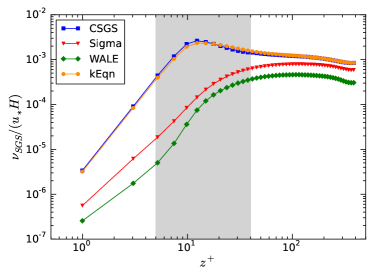
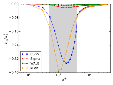
The SGS viscosities and stresses are the direct results of the SGS models, which are hence firstly studied. Figure 1 shows the profiles of the SGS viscosity $\nu_{SGS}$ and the major component $\tau_{13}$ of the SGS stresses (other components are negligibly small). The $\nu_{SGS}$ in the CSGS model denotes the $\nu_{SGS}$ in the baseline kEqn model. In the viscous sublayer, the SGS viscosity scales in all models with the distance as $\nu_{SGS}\sim z^{3}$, which agrees with the theoretical expectation Pope (2000). Nevertheless, the magnitudes differ by up to one order of magnitude, the smallest being from the WALE model and the biggest from the kEqn and CSGS model. Given that all models considered here are based on the eddy-viscosity assumption, $\tau=-2\nu_{SGS}|S|$, the difference in $\nu_{SGS}$ is translated into the SGS stress, as clearly shown in Fig. 1 (right). Interestingly, in the buffer layer, the differences of the SGS viscosity and stress among models are significantly higher than in other regions. Moreover, since the baseline model of the CSGS model is kEqn and the CSGS can be viewed simply as a correction to the kEqn model, the closeness in $\nu_{SGS}$ between these two models is expected and indicates that the constraint has a negligible effect on the SGS kinetic energy and viscosity. However, the constraint has a large impact on the SGS stress in the constrained region ($z^{+}<40$), as is shown in the profile of $\tau_{13}$. How the turbulence statistics are affected by the difference in the magnitude of $\nu_{SGS}$ and the correction from the constraint will be explained in the remainder of this section.

Figure 1: Profiles of the normalized SGS viscosity $\nu_{SGS}$ (left) and stress $\tau_{13}$ (right). The color markers correspond to different SGS models. The shaded region is the buffer layer ($z^{+}\in[5,40]$ or $z\in[0.013,0.1]H$). The colors and the shaded region represent the same variables in other figures.

Figure 2: Profiles of the mean streamwise velocity in wall units. The dashed line is the DNS data from  Moser, Kim, and Mansour (1999). Inset is a replicate of the buffer layer with X-axis in linear scale; note that the mean velocity based on the CSGS model best matches the DNS result.

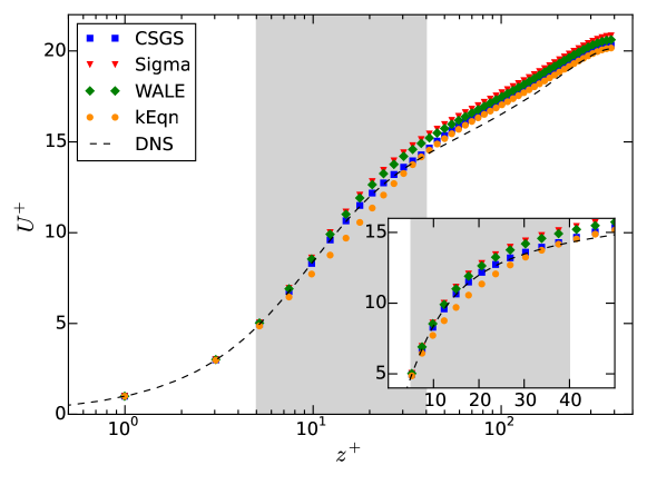
The profiles of the mean streamwise velocity in wall units, $U^{+}=U/u_{*}$, are shown in Fig. 2. All SGS models achieve a mean-velocity profile that agrees within a relative error of about 6% with the the DNS results. Moreover, a remarkably close match is found in the viscous sublayer for all models. In the logarithmic layer and outer layer, all profiles display an overestimation of the mean velocity, i.e., the log-layer mismatch problem. The mismatch in Sigma and WALE is negligibly greater than those in kEqn and CSGS. However, in the buffer layer, different models behave in distinct ways. The kEqn model underestimates the mean velocity while Sigma and WALE gradually overpredict it. The CSGS achieves the best mean velocity profile. In the whole constrained region, the mean velocity profile is in excellent agreement with the DNS results, since the constraint applied in the CSGS simulation is the mean Reynolds stress from the DNS simulation.

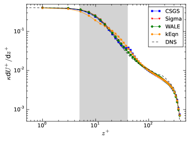
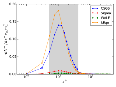
A more dynamically relevant quantity is the mean velocity gradient, which is plotted in Fig. 3 (left). Except for the kEqn model in the buffer layer and the CSGS model near the top of the constrained region, all profiles agree very well with the DNS results. The mismatch of the mean velocity profiles in the log layer and outer layer is also significantly reduced in the velocity gradient. It seems that the root of the log-layer mismatch in the mean velocity profile in the simulations lies in the inferior model performance in the buffer layer. Moreover, unlike in previous studies where the mismatch problem is claimed to be induced by the inaccurate SGS dissipations Porté-Agel, Meneveau, and Parlange (2000); Kawai and Larsson (2012); Wu and Meyers (2013), the profiles of the mean-flow SGS dissipations here (Fig. 3 right) does not show a noticeable correlation with the observed mismatch: although the SGS dissipation in both kEqn and CSGS are very high compared to others, the predictions of the mean velocity and its gradient are very close.

Figure 3: Profiles of the normalized velocity gradient (left) and the normalized mean-flow SGS dissipation $\tau_{13}\text{d}U/\text{d}z$ (right).

Consider now the force balance in the mean flow. Averaging the momentum equation for the streamwise velocity in time and in the horizontal (X and Y) directions, one obtains

$$\centering uw+\tau_{13}-\nu\frac{\text{d}U}{\text{d}z}=u_{*}^{2}(\frac{z}{H}-1),\@add@centering$$ (7)

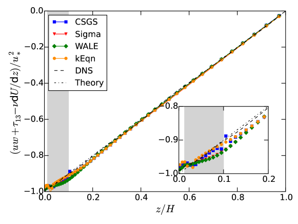
where the mean SGS stress is defined as $\tau_{13}=-\langle\nu_{SGS}\text{d}u/\text{d}z\rangle$. Note that the averaging operator $\langle\cdot\rangle$ is omitted in above equation. The derivation of this equation assumes temporal and horizontal statistical homogeneity, which is satisfied in the statistically stationary channel flow. Note that this relation is an exact integral form of the momentum equations and shows that, indepentent from the SGS modeling, the total stress is a linear function of the distance to the wall. Any deviation from this behavior is not due to the SGS model but to other numerical issues.

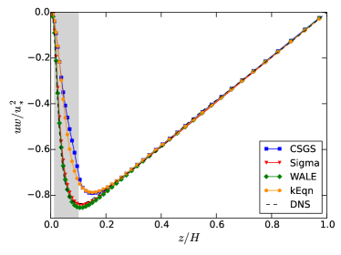
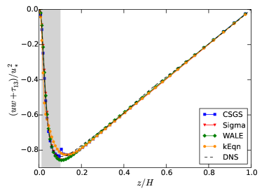
The total shear stress, and the resolved and full Reynolds shear stresses, are plotted in Fig. 4. Here only the $xz$ or $13$ component is shown. The other two shear components are theoretically zero. All total shear profiles agree very well with theoretical results, except in the near-wall region $z<0.2H$. In this region, the total shear profiles in the WALE and Sigma model deviate slightly further from the theoretical curve than in CSGS and kEqn, overall within 2% relative error. This deviation due to numerical errors is very small compared to that for other statistics, which hints a small numerical viscosity in the simulations.

In the $uw$ profile, WALE and Sigma are much closer to the DNS curve, while in the $uw+\tau_{13}$ profile all models perform very closely. From all above results, it seems that, among the variables in Eq. (7), $uw$ correlate highly with $\nu_{SGS}$, while the velocity gradient $\text{d}U/\text{d}z$ is a result of much more complicated mechanism, including the governing equations and the SGS models. This complexity makes it extremely difficult to solve the log-layer mismatch problem, and also indicates that ensuring correct SGS and Reynolds shear stresses is only a necessary but not a sufficient condition for accurately predicting the mean flow.

Figure 4: Profiles of the total shear stress (top), the resolved (bottom left) and full (bottom right) Reynolds shear stresses. The dash-dotted line corresponds to the theoretical result Eq. (7). The inset in the top figure is a zoom-in of the near-wall region.

The turbulence intensities are characterized by the resolved velocity variances, which are plotted in Fig. 5. Except for the streamwise variance $uu$ in WALE and Sigma, all other profiles show an underestimation compared to the DNS level and are almost the same in the outer layer. In the near wall region, WALE and Sigma overestimate $uu$ by up to 20% and resolve the variances $vv$ and $ww$ better than the other models. It is interesting that the CSGS model performs even worse in $uu$ than its baseline model kEqn, although CSGS predicts a better mean velocity profile(see Fig. 2). Note that the inaccurate predictions of variances are not necessarily due to the incorrectly modeled SGS dissipation, which can also be induced by the nonnegligible numerical viscosity inherent in the finite volume method. Overall, it is shown that different models result in significant differences in the buffer layer, including the location of the peaks.

Figure 5: Profiles of the resolved veloicty variances.

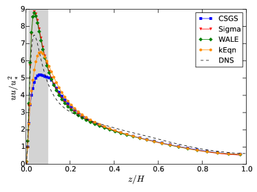
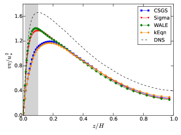
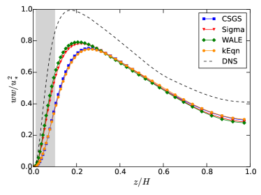
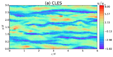
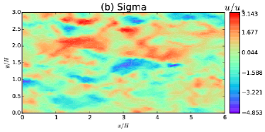
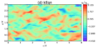
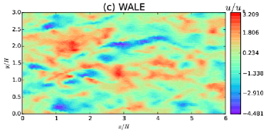
Figure 6 and 7 show the fields of instantaneous velocity fluctuations at $z/H=0.05$ (in the buffer layer) and $z/H=0.5$ (in the outer layer). It is clearly seen that the resolved turbulent structures are significantly different in the buffer layer for different models, while they are undistinguishable in the outer layer. In the buffer layer, the turbulence is dominated by the streamwise streaks in all models, but the streaks are much finer in Sigma and WALE. The reduced content in the near-wall flow structures for kEqn and CSGS may be due to the excessive over-estimation of the SGS dissipation, as shown in Fig. 3 (right).

Figure 6: Contour of instantaneous velocity fluctuation at $z/H=0.05$ (in the buffer layer). (a) CLES, (b) Sigma, (c) WALE, (d) kEqn. Turbulent structures are much finer for WALE and Sigma near the wall.

Figure 7: Contour of instantaneous velocity fluctuation at $z/H=0.5$ (in the outer layer). (a) CLES, (b) Sigma, (c) WALE, (d) kEqn. Turbulent structures are similar in the outer layer.

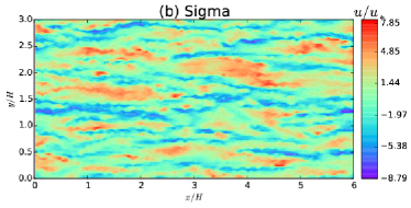
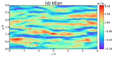
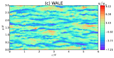
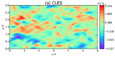
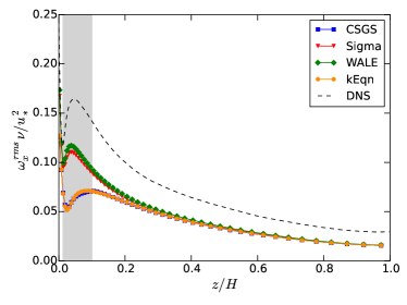
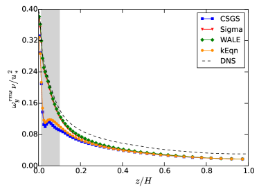
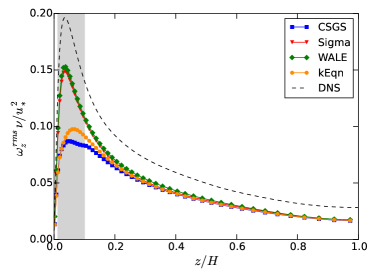
The fluctuations of vorticity are next analyzed. Vorticity fluctuations are thought to be more relevent to small-scale turbulent structures than velocity flucturations Moin and Kim (1982). Therefore, the vorticity fluctuations are considered as a better measure for the accuracy of SGS models. The profiles of the root-mean-square (RMS) of the vorticity fluctuations are shown in Fig. 8. The values for the WALE and Sigma model are considerably closer to the DNS results than for other models, notably in the buffer layer where the turbulence is the most intense. The local minimum and maximum in $\omega_{x}^{rms}$ are found in all models, meaning that the near-wall coherent structures (streamwise streaks and vortices) are well captured and are consistent with the contour plots in Fig. 6. The differences are in the magnitude of the fluctuations and the location of the local extremum. In the $\omega_{y}^{rms}$ profile, the WALE and Sigma model follow very closely the DNS data near the wall, while kEqn and CSGS result in an artificial local extremum. In $\omega_{x}^{rms}$ and $\omega_{z}^{rms}$, WALE and Sigma predict up to twice better in the buffer layer than kEqn and CSGS. In the outer layer, all vorticity components are clearly underestimated, whereas for the velocity variances the component $uu$ is well resolved by all models, as shown in Fig. 5. Again, it is shown that the CSGS model yields even worse results in fluctuations.

Figure 8: Profiles of the root-mean-square of the fluctuating vorticities.

To test the dependence of the results on the location of the constraint interface, the interface below which the constraint is imposed, we have performed a group of simulations with three interface locations, $z_{i}=0.01H,0.05H,0.1H$. These three locations are in the viscous sublayer, buffer and logarithmic layer, respectively. The results are compared with the ones from the simulation without constraint and from the DNS. To test whether the baseline model has influence on the constraint model, we employ here the WALE model as the baseline model. Other parameters are identical as in the previous simulations.

Figure 9: Profiles of the mean streamwise velocity in wall units for different locations of the constraint interface. The dashed line is the DNS data from Moser, Kim, and Mansour (1999). The shaded region is the buffer layer ($z^{+}\in[5,40]$ or $z\in[0.013,0.1]H$). The legend denotes the location of the constraint interface, below which the constraint is on.

Figure 10: Profiles of the normalized velocity gradient (left) and the normalized mean-flow SGS dissipation $\tau_{13}\text{d}U/\text{d}z$ (right).

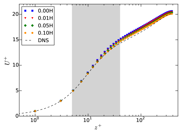
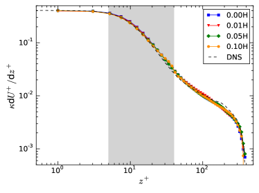
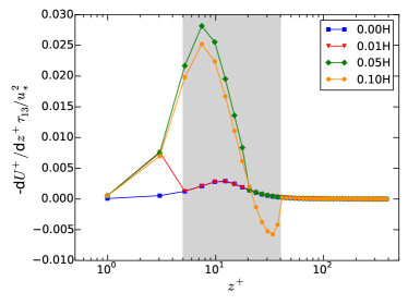
Figure 9 shows the mean streamwise velocity profiles for different constraint interface locations. It is shown that as the constraint interface moves away from the wall, the difference between the log layer and the DNS results becomes smaller. For $z_{i}=0.01H$, the profile is almost the same as the one from the simulation without constraint. These observations are in agreement with Chen et al. Chen et al. (2012), regardless of the pseudo-spectral method used in the simulations in the latter. However, the velocity gradient (Fig. 10 left), the second moments and the fluctuating vorticities display negligible difference for different interface locations. The interface location, nevertheless, changes significantly the mean-flow SGS dissipation in the near-wall region, especially the buffer layer, as shown in Fig. 10 (right). Here for WALE, the constraint increases the SGS dissipation in the buffer layer, whereas, for kEqn, it decreases the SGS dissipation (Fig. 3 right). This provides strong evidence that in the buffer layer, the kEqn model overpredict the SGS dissipation while WALE results in an under-estimation.

V Discussion and conclusions

In this paper a comparative study of various SGS models was conducted by performing a compaign of OpenFOAM finite-volume wall-resolved LES simulations. The canonical channel flow at $Re_{\tau}=395$ was chosen as the working flow and the DNS results from Moser et al. Moser, Kim, and Mansour (1999) as a reference. Four SGS models were studied, including kEqn, WALE, Sigma and CSGS. The geometry was the same as in the paper by Moser et al. Moser, Kim, and Mansour (1999), $(2\pi\times\pi\times 2)H$, with a resolution of $(96\times 96\times 96)$ and $z^{+}\simeq 1$ for the first point. A constant pressure gradient was employed as the driving force of the flow. The CSGS and Sigma model, together with the source term, were implemented in OpenFOAM 3.0.1. The new implementation strategy for the CSGS model can be easily incorporated into the existing LES codes.

By analyzing the turbulence statistics up to second order, significant differences were found in the SGS models, especially in the buffer layers where the turbulence intensities were the strongest. The WALE and Sigma models result in much stronger velocity and vorticity fluctuations, as well as much finer flow structures, near the wall. This may be explained by the significantly smaller SGS viscosity and the resultant smaller SGS dissipation inherent in these two models. Compared to its baseline model kEqn, the CSGS with constraints on the mean Reynolds shear stress had a marginal improvement in the mean velocity but resulted in a slightly worse prediction on the fluctuations. Compared to the good results achieved with a spectral code in Chen et al. (2012), the deteriorated performance of CSGS here is probably due to the finite volume method used in the simulations, which is also consistent with the observations by Verma et al. Verma, Park, and Mahesh (2013). This seems consistent with the arguments in Meneveau (1994) that ensuring correct Reynolds shear stresses is only a necessary but not a sufficient condition for yielding accurate statistics. Overall, these differences reveal the crucial role of the SGS models in the buffer layer in wall-resolved LES simulations and more generally in the near-wall regions.

The SGS models considered in the paper also share common features. First, in the log layer and outer layer, all models resulted in a mean velocity profile which agrees reasonably well with the DNS results. A slight log-layer mismatch is present in each model. Different from the wall-modelled simulations in previous studies Porté-Agel, Meneveau, and Parlange (2000); Kawai and Larsson (2012); Wu and Meyers (2013), the mismatch here was shown to have little correlation with the SGS viscosity and dissipation. The underlying mechanisms for the mismatch are much more complicated. Second, most turbulence statistics are underestimated compared to the DNS data. This systematic underestimation is likely a result of the lesser resolutions, but may also be attributed to a fundamental problem intrinsic in the eddy-viscosity family, i.e., the assumption that the SGS stress is linearly proportional to the rate-of-strain tensor is incorrect Meneveau and Katz (2000). Nonlinear gradient models had been proprosed Liu, Meneveau, and Katz (1994) but they were reported to achieve only a marginal improvement. Another important missing component in the current majority SGS models is stochasticity. Although governed by deterministic equations, turbulence is stochastic. Previous studies  Marstorp, Brethouwer, and Johansson (2007); Zidikheri and Frederiksen (2010); Rasam, Brethouwer, and Johansson (2014) already showed in certain cases that stochastic effects improve the fluctuation magnitudes and their anisotropy. Hence, building appropriate practical stochastic SGS models is desired to adequately capture the random backscattering of the SGS flow motions.

A constantly ignored quantity in the study of SGS models is the pressure fluctuation, which is often considered as less relevant to the flow dynamics. As Pope indicated in Pope (2000), “the primary effect of the fluctuating pressure is to redistribute the energy among the components – to extract energy from $\langle uu\rangle$ and transfer it to $\langle vv\rangle$ and $\langle ww\rangle$.” However, the interaction between the SGS model and the resolved pressure fluctuation is unknown. More than 30 years ago, Moin and Kim Moin and Kim (1982) had already speculated that an appreciable portion of the pressure fluctuation may reside in SGS motions and that “the splatting effect is an important property of the flow in the vicinity of the walls and should be taken into account in the modeling of near-wall turbulence.” Different from the “primary” effect on the bulk flow, the splatting effect denotes the transfer of energy from $\langle ww\rangle$ to the other two components due to the presence of the wall. These two types of effects are seldom considered in most SGS models. According to the results from WALE and Sigma models, the energy from $\langle uu\rangle$ seems to be incorrectly transferred to the other two components, resulting in an overprediction of $\langle uu\rangle$. This transfer of energy is mainly affected through the pressure-rate-of-strain tensor $\langle pS_{ij}\rangle$. To the author’s best knowledge, no DNS or experimental data are available for this tensor, making it difficult to check the above speculation. Nevertheless, the discovery of a relationship between the pressure-rate-of-strain tensor and the velocity-accelaration correlation Pope (2014) offers a feasible way for the experimentalists to gain insights into this quantity and to check whether the normal SGS stress should be directly modeled.

References

- Lesieur and Métais (1996) M. Lesieur and O. Métais, “New trends in large-eddy simulations of turbulence,” Annu. Rev. Fluid Mech. 28, 45–82 (1996).
- Meneveau and Katz (2000) C. Meneveau and J. Katz, “Scale-invariance and turbulence models for large-eddy simulation,” Annu. Rev. Fluid Mech. 32, 1–32 (2000).
- Smagorinsky (1963) J. Smagorinsky, “General circulation experiments with the primitive equations. I. the basic experiment,” Mon. Weather Rev. 91, 99–164 (1963).
- Lilly (1967) D. K. Lilly, “The representation of small-scale turbulence in numerical simulation experiments,” Proc. IBM Scientific Computing Symp. Environ. Sci. , 195 (1967).
- Schumann (1975) U. Schumann, “Subgrid scale model for finite difference simulations of turbulent flows in plane channels and annuli,” J. Comput. Phys. 18, 376–404 (1975).
- Germano et al. (1991) M. Germano, U. Piomelli, P. Moin, and W. H. Cabot, “A dynamic subgrid-scale eddy viscosity model,” Phys. Fluids A3, 1760–1765 (1991).
- Porté-Agel, Meneveau, and Parlange (2000) F. Porté-Agel, C. Meneveau, and M. B. Parlange, “A scale-dependent dynamic model for large-eddy simulation: application to a neutral atmospheric boundary layer,” J. Fluid Mech. 415, 261–284 (2000).
- Trias et al. (2015) F. X. Trias, D. Folch, A. Gorobets, and A. Oliva, “Building proper invariants for eddy-viscosity subgrid-scale models,” Phys. Fluids 27, 065103 (2015).
- Nicoud and Ducros (1999) F. Nicoud and F. Ducros, “Subgrid-scale stress modelling based on the square of the velocity gradient tensor,” FLow, Turbulence and Combustion 62, 183–200 (1999).
- Vreman (2004) A. W. Vreman, “An eddy-viscosity subgrid-scale model for turbulent shear flow: Algebraic theory and applications,” Phys. Fluids 16, 3670–3681 (2004).
- Verstappen (2011) R. Verstappen, “When does eddy viscosity damp subfilter scales sufficiently?” J. Sci. Comput. 49, 94–110 (2011).
- Nicoud et al. (2011) F. Nicoud, H. B. Toda, O. Cabrit, S. Bose, and J. Lee, “Using singular values to build a subgrid-scale model for large eddy simulations,” Phys. Fluids 23, 085106 (2011).
- Sullivan, McWilliams, and Moeng (1994) P. P. Sullivan, J. C. McWilliams, and C.-H. Moeng, “A subgrid-scale model for large-eddy simulation of planetary boundary-layer flows,” Boundary-Layer Meteorol. 71, 247–276 (1994).
- Lévêque et al. (2007) E. Lévêque, F. Toshi, L. Shao, and J.-P. Bertoglio, “Shear-improved smagorinsky model for large-eddy simulation of wall-bounded turbulent flows,” J. Fluid Mech. 570, 491–502 (2007).
- Chen et al. (2012) S. Chen, Z. Xia, S. Pei, J. Wang, Y. Yang, Z. Xiao, and Y. Shi, “Reynolds-stress-constrained large-eddy simulation of wall-bounded turbulent flows,” J. Fluid Mech. 703, 1–28 (2012).
- Yoshizawa (1985) A. Yoshizawa, “A statistically-derived subgrid-scale kinetic energy model for the large-eddy simulations of turbulent flows,” Journal of the Physical Society of Japan 54, 2834–2839 (1985).
- de Villiers (2006) E. de Villiers, The Potential of Large Eddy Simulation for the Modeling of Wall Bounded Flows, Ph.D. thesis, Imperial College of Science, Technology and Medicine (2006).
- Shi, Xiao, and Chen (2008) Y. Shi, Z. Xiao, and S. Chen, “Constrained subgrid-scale stress model for large eddy simulation,” Phys. Fluids 20, 011701 (2008).
- Jiang et al. (2013) Z. Jiang, Z. Xiao, Y. Shi, and S. Chen, “Constrained large-eddy simulation of wall-bounded compressible turbulent flows,” Phys. Fluids 25, 106102 (2013).
- Zhao et al. (2014) Y. Zhao, Z. Xia, Y. Shi, Z. Xiao, and S. Chen, “Constrained large-eddy simulation of laminar-turbulent transition in channel flow,” Phys. Fluids 26, 095103 (2014).
- Moser, Kim, and Mansour (1999) R. D. Moser, J. Kim, and N. N. Mansour, “Direct numerical simulation of turbulent channel flow up to ,” Phys. Fluids 11, 943 (1999).
- 3.0. (1) O. 3.0.1, “http://openfoam.org/release/3-0-1/,” .
- Robertson et al. (2015) E. Robertson, V. Choudhury, S. Bhushan, and D. K. Walters, “Validation of OpenFOAM numerical methods and turbulence models for incompressible bluff body flows,” Comput. Fluids 123, 122–145 (2015).
- Pope (2000) S. B. Pope, Turbulent Flows (Cambridge University Press, 2000).
- Kawai and Larsson (2012) S. Kawai and J. Larsson, “Wall-modeling in large eddy simulation: Length scales, grid resolution, and accuracy,” Phys. Fluids 24, 015105 (2012).
- Wu and Meyers (2013) P. Wu and J. Meyers, “A constraint for the subgrid-scale stresses in the logarithmic region of high reynolds number turbulent boundary layers: A solution to the log-layer mismatch problem,” Phys. Fluids 25, 015104 (2013).
- Moin and Kim (1982) P. Moin and J. Kim, “Numerical investigation of turbulent channel flow,” J. Fluid Mech. 118, 341–377 (1982).
- Verma, Park, and Mahesh (2013) A. Verma, N. Park, and K. Mahesh, “A hybrid subgrid-scale model constrained by reynolds stress,” Phys. Fluids 25, 110805 (2013).
- Meneveau (1994) C. Meneveau, “Statistics of turbulence subgrid-scale stresses: Necessary conditions and experimental tests,” Phys. Fluids 6, 815–833 (1994).
- Liu, Meneveau, and Katz (1994) S. Liu, C. Meneveau, and J. Katz, “On the properties of similarity subgrid-scale models as deduced from measurements in a turbulent jet,” J. Fluid Mech. 275, 83–119 (1994).
- Marstorp, Brethouwer, and Johansson (2007) L. Marstorp, G. Brethouwer, and A. V. Johansson, “A stochastic subgrid model with application to turbulent flow and scalar mixing,” Phys. Fluids 19, 035107 (2007).
- Zidikheri and Frederiksen (2010) M. Zidikheri and A. S. Frederiksen, “Stochastic subgrid-scale modelling for non-equilibrium geophysical fluids,” Phil. Trans. R. Soc. A 368, 145–160 (2010).
- Rasam, Brethouwer, and Johansson (2014) A. Rasam, G. Brethouwer, and A. V. Johansson, “A stochastic extension of the explicit algebraic subgrid-scale models,” Phys. Fluids 26, 055113 (2014).
- Pope (2014) S. B. Pope, “The determination of turbulence-model statistics from the velocity-acceleration correlation,” J. Fluid Mech. 757, R1 1–9 (2014).