Exact fluctuations of nonequilibrium steady states
from approximate auxiliary dynamics

Abstract

We describe a framework to reduce the computational effort to evaluate large deviation functions of time integrated observables within nonequilibrium steady states. We do this by incorporating an auxiliary dynamics into trajectory based Monte Carlo calculations, through a transformation of the system’s propagator using an approximate guiding function. This procedure importance samples the trajectories that most contribute to the large deviation function, mitigating the exponential complexity of such calculations. We illustrate the method by studying driven diffusion and interacting lattice models in one and two spatial dimensions. Our work offers an avenue to calculate large deviation functions for high dimensional systems driven far from equilibrium.

Much like their equilibrium counterparts, fluctuations about nonequilibrium steady states encode physical information about a system. This is illustrated by the discovery of the fluctuation theorems Crooks (1999); Kurchan (1998); Lebowitz and Spohn (1999); Gallavotti and Cohen (1995), thermodynamic uncertainty relations Barato and Seifert (2015); Gingrich et al. (2016), and extensions of the fluctuation-dissipation theorem to systems far-from-equilibrium Harada and Sasa (2005); Speck and Seifert (2006); Baiesi et al. (2009); Marconi et al. (2008). Large deviation functions provide a general mathematical framework within which to characterize and understand non-equilibrium fluctuations Touchette (2009) and their evaluation has underpinned much recent progress in understanding driven systems Harris and Schütz (2007); Mehl et al. (2008); Prados et al. (2011); Tsobgni Nyawo and Touchette (2016a). However, the current Monte Carlo methods such as the cloning algorithm Grassberger (2002); Del Moral and Garnier (2005); Giardinà et al. (2006); Giardina et al. (2011); Cérou et al. (2011); Nemoto et al. (2016) or transition path sampling Bolhuis et al. (2002), exhibit low statistical efficiency when accessing rare fluctuations that are needed to compute them  Nemoto et al. (2016); Ray et al. (2018). This has limited the numerical application of large deviation theory to idealized model systems with relatively few degrees of freedom.

In principle, these difficulties can be eliminated through the use of importance sampling. A formally exact importance sampling can be derived through Doob’s h-transform, although this requires the exact eigenvector of the tilted operator that generates the biased path ensemble Doob (1984); Chetrite and Touchette (2015); Jack and Sollich (2010). As this is not practical, approximate importance sampling schemes have been introduced Klymko et al. (2017); Nemoto et al. (2016, 2017), including a sophisticated iterative algorithm to improve sampling based on feedback and control Nemoto et al. (2016, 2017).

In this Letter, we will show that guiding distribution functions (GDF), used to implement importance sampling in diffusion Monte Carlo (DMC) calculations of quantum ground states, can be extended to provide an approximate, but improvable, importance sampling for the simulation of nonequilibrium steady states. We show the potential of the GDF method by computing the large deviation functions of time integrated currents at large bias values that capture very rare fluctuations within two widely-studied models: a driven diffusion model and an interacting lattice model. As examples of GDFs, we use analytical expressions as well GDFs determined from a generalized variational approximation SI . The variational approach provides a procedure to generate guiding functions for arbitrary models of interest.

We begin with a short review of the formalism of large deviation functions, drawing connections to the ideas of DMC used in this work. We consider steady states generated by a Markovian dynamics

$$\partial_{t}p_{t}(\mathcal{C})=\mathcal{W}p_{t}(\mathcal{C})$$ (1)

where $p_{t}(\mathcal{C})$ is the probability of a configuration of the system, $\mathcal{C}$, at a time $t$, and $\mathcal{W}$ is a linear operator. Provided $\mathcal{W}$ is irreducible, it generates a unique steady state in the long time limit that in general produces non-vanishing currents and whose configurations do not necessarily follow a Boltzmann distribution. We consider the fluctuations of observables of the form ${\mathcal{O}}=\sum_{t=1}^{t_{N}}o(\mathcal{C}_{t+},\mathcal{C}_{t-})$, where $o$ is an arbitrary function of configurations at adjacent times, $t+$ and $t-$. Within the steady-state, the fluctuations of a time integrated observable can be characterized by a generating function,

$$e^{\psi(\lambda)t_{N}} = \left<e^{-\lambda\mathcal{O}}\right>=\sum_{\mathscr{C}(t_{N})}P[\mathscr{C}(t_{N})]e^{-\lambda\mathcal{O}}$$ (2)

where $\psi(\lambda)$ is the large deviation function, $\lambda$ is a counting field conjugate to $\mathcal{O}$, and $P[\mathscr{C}(t_{N})]$ is the likelihood of a given trajectory $\mathscr{C}(t_{N})=\{\mathcal{C}_{0},\mathcal{C}_{1},\dots,\mathcal{C}_{t_{N}}\}$. Derivatives of the large deviation function with respect to $\lambda$ yield the time-intensive cumulants of $\mathcal{O}$.

In principle, the large deviation function is computable from the largest eigenvalue of a tilted operator $\mathbb{W}_{\lambda}$, i.e., $\mathbb{W}_{\lambda}|\Xi\rangle=\psi(\lambda)|\Xi\rangle$ where $|\Xi\rangle$ ($\langle\Xi|$) is the corresponding dominant right (left) eigenvector Lebowitz and Spohn (1999). In the discreet case, $\mathbb{W}_{\lambda}(\mathcal{C},\mathcal{C}^{\prime})=\mathcal{W}(\mathcal{C},\mathcal{C}^{\prime})e^{-\lambda o(\mathcal{C},\mathcal{C}^{\prime})}(1-\delta_{\mathcal{C},\mathcal{C}^{\prime}})-R(\mathcal{C})\delta_{\mathcal{C},\mathcal{C}^{\prime}}$, where $R(\mathcal{C})=\sum_{\mathcal{C}\neq\mathcal{C}^{\prime}}\mathcal{W}(\mathcal{C},\mathcal{C}^{\prime})$ is the exit rate. For $\lambda=0$, the tilted operator is Markovian and $\psi(0)=0$ due to normalization. However, in general $\mathbb{W}_{\lambda}$ does not conserve probability. To sample the dynamics generated by $\mathbb{W}_{\lambda}$ with Markov chain Monte Carlo, for example, within the cloning algorithm or transition path sampling, one must track the normalization with additional weights Foulkes et al. (2001). This normalization grows exponentially with $\lambda$. Thus, the associated weights in Monte Carlo algorithms have an exponentially growing variance, and this is the origin of low statistical efficiency.

The goal of importance sampling is to reduce this variance, and this can be carried out by transforming the dynamics to restore the normalization of the tilted operator. Mathematically, we achieve this through Doob’s h-transform,

$$\mathcal{W}_{\lambda}(\mathcal{C},\mathcal{C}^{\prime})=\Xi(\mathcal{C}){\mathbb{W}}_{\lambda}(\mathcal{C},\mathcal{C}^{\prime})\Xi^{-1}(\mathcal{C}^{\prime})-\psi(\lambda)\,,$$ (3)

with $\Xi(\mathcal{C})=\langle\Xi|\mathcal{C}\rangle$. We see that $\sum_{\mathcal{C}}\mathcal{W}_{\lambda}(\mathcal{C},\mathcal{C}^{\prime})=0$, since $\sum_{\mathcal{C}}\Xi(\mathcal{C}){\mathbb{W}}_{\lambda}(\mathcal{C},\mathcal{C}^{\prime})=\psi(\lambda)\Xi(\mathcal{C}^{\prime})$. The auxiliary dynamics generated by $\mathcal{W}_{\lambda}$ is thus the optimal dynamics to sample, since the normalization of $\mathcal{W}_{\lambda}$ is completely independent of configuration. Unfortunately, it requires $\langle\Xi|$ to be known explicitly.

We can, however, approximate $\langle\Xi|$ and use it to carry out an approximate h-transform in order to importance sample trajectories. This is the basic technique in this work and is analogous to using guiding wavefunctions to importance sample in DMC Ceperley and Alder (1980); Foulkes et al. (2001). The basic DMC algorithm is equivalent to the cloning algorithm with $\mathbb{W}_{\lambda}$ replaced by the quantum Hamiltonian and the large deviation function $\psi(\lambda)$ and eigenvector $|\Xi\rangle$ replaced by the ground-state energy and wavefunction respectively. The main technical difference is that unlike the Hamiltonians in DMC, ${\mathbb{W}}_{\lambda}$ is not, in general, Hermitian. We focus here on the use of GDFs in the cloning algorithm, though it can also be used with transition path sampling.

The cloning algorithm computes the large deviation function as the mixed estimator

$$\psi(\lambda)\sim\frac{1}{t_{N}}\ln\langle\mathbbm{1}|e^{t_{N}\mathbb{W}_{\lambda}}|p_{0}\rangle,$$ (4)

where $\langle\mathbbm{1}|=\sum_{\mathcal{C}}\langle\mathcal{C}|$ is the uniform left vector, $|p_{0}\rangle$ is an arbitrary initial state (not orthogonal to the final state) and $\sim$ denotes a long time limit. Since the full propagator $\exp[t_{N}\mathbb{W}_{\lambda}]$ is not known explicitly, it is approximated by short-time pieces using a Trotter decomposition, which can be explicitly sampled Foulkes et al. (2001). The distribution $p_{t}$ is represented by an ensemble of walkers, and the propagation $|p_{t+\Delta t}\rangle=\exp[{\Delta t\mathbb{W}_{\lambda}}]|p_{t}\rangle$ is obtained via Monte Carlo sampling. As discussed, the sampling procedure accounts for the unnormalized $\mathbb{W}_{\lambda}$ by keeping weights on the walkers. To avoid a divergence of these weights, they are redistributed at each iteration, a procedure known as cloning (or branching in DMC) Giardinà et al. (2006); Ray et al. (2018).

To importance sample, we now construct an auxiliary dynamics from an approximate GDF, $\langle\tilde{\Xi}|=\sum_{\mathcal{C}}\tilde{\Xi}(\mathcal{C})\langle\mathcal{C}|$. We transform Eq. 4 using the GDF via the diagonal matrix $\hat{\Xi}=\sum_{\mathcal{C}}\tilde{\Xi}(\mathcal{C})|\mathcal{C}\rangle\langle\mathcal{C}|$ such that

$$\psi(\lambda)\sim\frac{1}{t_{N}}\ln\langle\mathbbm{1}|\hat{\Xi}^{-1}[\hat{\Xi}e^{t_{N}\mathbb{W}_{\lambda}}\hat{\Xi}^{-1}]\hat{\Xi}|p_{0}\rangle.$$ (5)

The resulting transformed propagator, $\tilde{W}_{\lambda}(\mathcal{C},\mathcal{C}^{\prime})=\tilde{\Xi}(\mathcal{C}){\mathbb{W}}_{\lambda}(\mathcal{C},\mathcal{C}^{\prime})\tilde{\Xi}^{-1}(\mathcal{C}^{\prime})$, generates the importance sampled dynamics. Note that $\tilde{W}_{\lambda}$ is only Markovian if $\langle\tilde{\Xi}|=\langle{\Xi}|$, which is generally not the case, and thus the problem of normalization persists. However, if $\langle\tilde{\Xi}|$ strongly overlaps with $\langle{\Xi}|$, the corresponding exponential growth of the variance is diminished. The key to efficient sampling is thus reduced to determining appropriate approximate GDFs for specific problems.

We now turn to a numerical assessment of the GDF auxiliary dynamics importance sampling. Here, an important metric is the efficacy of the auxiliary dynamics. This can be quantified in terms of the statistical efficiency of sampling. For the cloning algorithm, the measure of interest is the number of correlated walkers $N_{\mathrm{c}}$ Nemoto et al. (2016). In the case of perfect sampling, using the exact auxiliary dynamics, $N_{\mathrm{c}}$ is equal to 1. In the other limit, if all walkers are correlated, $N_{\mathrm{c}}=N_{\mathrm{w}}$, the number of walkers used in the simulation.

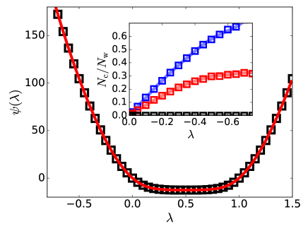
Figure 1: Large deviation function for the entropy production of a driven brownian particle on a periodic potential with $v_{o}=2$, $f=12.5$. The main figure shows the functions computed with exact diagonalization (red) and DMC (black). The inset shows the fraction of correlated walkers without GDF (blue), or with GDF from an instanton approximation to the auxiliary process (red) or the exact auxiliary process (black).

For illustrative purposes, we first consider fluctuations of the entropy production of a driven brownian particle in a periodic potential, a paradigmatic model in nonequilibrium statistical mechanics. The equation of motion for the position (on a ring) $\theta$, is $\partial_{t}{\theta}=F(\theta)+\eta\,$, with $F(\theta)=f-\partial_{\theta}V(\theta)$, where $f$ is a constant, nonconservative force, and $V(\theta)=v_{o}\cos(\theta)$ is a periodic potential Seifert (2012). The random force, $\eta$, satisfies $\langle\eta(t)\rangle=0\quad$ and $\langle\eta(t)\eta(t^{\prime})\rangle=2\delta(t-t^{\prime})$. The entropy production can be computed from $\sigma(t_{N})t_{N}=\int_{0}^{t_{N}}f\dot{\theta}(\tau)\mathrm{d}\tau$, which is linearly proportional to the current around the ring SI .

The tilted operator for this model is obtained by absorbing the biasing term $\exp[-\lambda t_{N}\sigma(t)]$ into the bare Fokker-Planck propagator, $\mathcal{W}=\partial_{\theta}^{2}-\partial_{\theta}F(\theta)$, giving

$${\mathbb{W}}_{\lambda}=\mathcal{W}+2f\lambda\partial_{\theta}+f\lambda(f\lambda-F(\theta)).$$ (6)

The last term breaks normalization and must be accommodated through branching. The first two terms represent a drift-diffusion process, configurations for which can generated via an associated Langevin equation,

$$\partial_{t}{\theta}=F(\theta)-2f\lambda+\eta.$$ (7)

Importance sampling this system with a GDF, $\tilde{\Xi}(\theta)$, produces the transformed propagator

$$\tilde{W}_{\lambda}=\mathcal{W}+2\partial_{\theta}[f\lambda-\partial_{\theta}\ln\tilde{\Xi}(\theta)]+\tilde{\Xi}^{-1}(\theta){\mathbb{W}}_{\lambda}^{\dagger}\tilde{\Xi}(\theta),$$ (8)

where the adjoint operator is defined as ${\mathbb{W}}_{\lambda}^{\dagger}=F(\theta)(\partial_{\theta}-f\lambda)+(\partial_{\theta}-f\lambda)^{2}$ SI . Importance sampled trajectories for $\tilde{W}_{\lambda}$ can thus be generated via a Langevin dynamics similar to Eq. 7, but with an additional force $2\partial_{\theta}\ln\tilde{\Xi}(\theta)$, and branching weight $\tilde{\Xi}^{-1}(\theta){\mathbb{W}}_{\lambda}^{\dagger}\tilde{\Xi}(\theta)$. Note that since the components of the left eigenvector of ${\mathbb{W}}_{\lambda}$ are equal to the components of the right eigenvector of its adjoint ${\mathbb{W}}^{\dagger}_{\lambda}$, if $\tilde{\Xi}(\theta)=\Xi(\theta)$, the branching term is equal to $\psi(\lambda)$.

For this simple one particle system we can determine the optimal GDF by diagonalizing ${\mathbb{W}}_{\lambda}$ in a plane wave basis Tsobgni Nyawo and Touchette (2016b); SI . To illustrate the behavior when an approximate GDF, we also consider a GDF obtained from an instantonic solution to the eigenvalue equation, which captures the correct limiting behavior of $\Xi(\theta)$ at large $\lambda$, where $\Xi(\theta)$ is just a constant Tsobgni Nyawo and Touchette (2016b).

Shown in Fig. 1 is the large deviation function computed from exact diagonalization, and cloning algorithm calculations without a GDF, with the optimal GDF, and with the instantonic GDF. All methods converge $\psi(\lambda)$ to good accuracy over the range of $\lambda$, and illustrate the fluctuation theorem symmetry $\psi(\lambda)=\psi(1-\lambda)$. However, the statistical effort required to converge the different Monte Carlo calculations varies significantly. This is summarized in the inset of Fig. 1, which shows $N_{\mathrm{c}}$ as a function of $\lambda$. The number of correlated walkers increases exponentially without a guiding function, but plateaus if the instantonic guiding function is used. Using the optimal GDF results in walkers that maintain equal weights and stay completely independent, with $N_{\mathrm{c}}=1$ for all times and all $\lambda$’s.

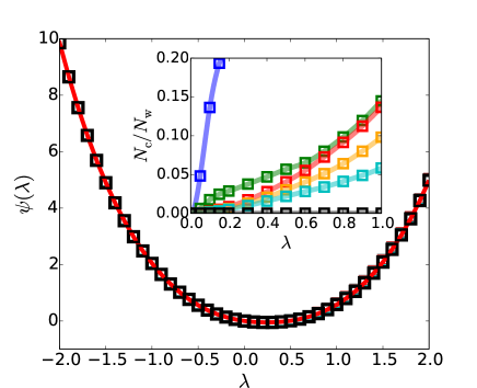
Figure 2: Large deviation function for the mass current of an open simple exclusion process. The main figure shows the functions computed with exact diagonalization (red) and DMC (black). The inset shows the fraction of correlated walkers without guiding functions (blue), or with GDF from approximations to the auxiliary process using a uniform GDF (green) or clusters of 1 (red), 2 (orange), 4 (cyan) and 8 (black) sites.

To explore our framework in different context, we now consider an interacting many-body problem on a lattice, namely the current fluctuations of a simple exclusion process (SEP) Schmittmann and Zia (1995). The SEP models transport on a lattice with $L$ sites, defined by a set of occupation numbers, $n_{i}=\{0,1\}$, e.g. $\mathcal{C}=\{0,1,..,1,1\}$. The tilted propagator, $\mathbb{W}_{\lambda}$, has elements corresponding to rates to insert and remove particles at the boundaries if the model is open, with insertion rates $\alpha$ and $\gamma$, and removal rates $\beta$ and $\nu$. Within the bulk of the lattice, particles move to the right with rate $p$ and to the left with rate $q$, subject to the constraint of single site occupancy. The hard core constraint results in correlations between particles moving on the lattice. We consider the large deviation function for mass currents, $Q(t_{N})$, equal to the number of particle hops to the left minus the number of hops to the right,

$$Q(t_{N})=\sum_{t=0}^{t_{N}-1}\sum_{i=0}^{L-1}\delta_{i+1}(t+1)\delta_{i}(t)-\delta_{i}(t+1)\delta_{i+1}(t)$$ (9)

where $\delta_{i}$ is the Kronecker delta function and the sum runs over the lattice site and $t_{N}$. The propagator is thus dressed by a factor of $\exp[-\lambda Q(t_{N})]$. Note that the summand is $=0,\pm 1$ depending on particle displacement.

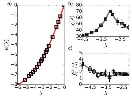
Figure 3: Large deviation function for the mass current of a closed 2$d$ asymmetric exclusion process. a) Large deviation function computed from DMC with importance sampling. b) Susceptibility for current fluctuations as a function of $\lambda$. c) Ratio of the fraction of independent walkers with importance sampling, $f_{\mathrm{I}}^{IS}$, and without importance sampling, $f_{\mathrm{I}}$.

For all but the smallest lattices, direct diagonalization of ${\mathbb{W}}_{\lambda}$ is impossible, as the size of the matrix scales exponentially with $L$. However, we can find an approximate set of eigenvectors using a cluster based mean-field approximation SI . For example, we can write $|\tilde{\Xi}\rangle$ as product state of single sites expanded in a basis of single particle states, $|\tilde{\Xi}\rangle=\prod_{i=1}^{L}\sum_{n=0,1}\xi_{i}(n)|n_{i}\rangle$ where $\xi_{i}(n)$ are the site expansion coefficients. These can be obtained numerically from the mean-field equations through a generalized variational principle since ${\mathbb{W}}_{\lambda}$ is not Hermitian (SI), where the stationary solution is found through self-consistent iteration. Similarly, one can consider a product state of clusters of sites, or a cluster mean-field. Increasing the size of the cluster systematically improves the GDF.

Figure 2 shows the results of using the cluster mean-field ansatz as the GDF for clusters of different size. We find that for an $L=8$ lattice, symmetric SEP model , all cloning calculations agree with the numerically exact result, and again illustrate fluctuation theorem symmetry, with $\psi$ symmetric about half of the current’s affinity Lebowitz and Spohn (1999). The statistical effort needed to converge each calculation is decreased by several orders of magnitude when a GDF is used. As shown in the inset of Fig. 2, even with an auxiliary dynamics computed from the single-site mean field theory, the fraction of independent walkers, $f_{\mathrm{I}}=1-N_{\mathrm{c}}/N_{\mathrm{w}}$, is increased by a factor of 40, and this efficiency is systematically improved with auxiliary dynamics computed from larger cluster states. As before, if the exact auxiliary process is used, corresponding to a cluster of 8 sites, $N_{\mathrm{c}}=1$ for all times and all $\lambda$’s.

As a third illustration of the auxiliary dynamics framework, we consider a 2D generalization of a closed SEP model in the presence of a weak external field that biases transport in one direction SI . This system has been considered recently Tizón-Escamilla et al. (2017), where it was found that its large deviation function for current fluctuations in the direction of the driving exhibits a dynamical phase transition. For small $\lambda$, the system is in a homogeneous phase, while for large negative $\lambda$ the system phase separates, forming a traveling wave in the direction of the biased current. We find critical behavior for a 12$\times$12 lattice as illustrated in Figs. 3a,b, where for $\lambda\approx-3$ the fluctuations in the current, $\chi(\lambda)=d^{2}\psi/d\lambda^{2}$, are maximized and presumed to diverge in the infinite system limit . Beyond this critical value, the state of the system is fluctuation dominated, and as such serves as a good test of our importance sampling methodology. Shown in Fig. 3c is the ratio of the fraction of independent walkers, $f_{\mathrm{I}}$, computed using a 4$\times$2 sites cluster mean field GDF and without importance sampling, as a function of $\lambda$. For small $|\lambda|$ the bare dynamics is capable of sampling the biased distribution and the enhancement from importance sampling is $\sim 2$. However, even for the traveling wave state, where the system is not well described by mean field theory, we find an increased sampling efficiency by a factor of 2-4 over bare sampling SI . This result shows that even a poor approximation to the steady-state using the cluster approach is able to aid the convergence of $\psi(\lambda)$.

Beyond these specific examples, we emphasize that the guiding framework we have described is general and is not restricted to the models we have considered. For example, we can consider importance sampling an $N$-particle interacting continuum dynamics generated by a Fokker-Planck operator $\mathcal{W}$ for an arbitrary many-body force $\mathbf{F}_{i}({\bf r}_{1},\ldots,{\bf r}_{N})$ in $d$ dimensions. The GDF in this case is an $N$-particle function $\tilde{\Xi}(\mathbf{r}_{1},\ldots,\mathbf{r}_{N})$ and the transformed tilted operator for the large deviation function for the total mass current vector $\mathbf{J}(t_{N})=\sum_{i}\int_{0}^{t_{N}}\dot{\mathbf{r}}_{i}(\tau)d\tau$,

$$\tilde{W}_{\bm{\lambda}}= \sum_{i}\nabla_{i}^{2}-\nabla_{i}\cdot\left[\mathbf{F}_{i}({\bf r}_{1},\ldots,{\bf r}_{N})-2\bm{\lambda}+2\nabla_{i}\ln{\tilde{\Xi}}\right]$$

$$+\tilde{\Xi}^{-1}\mathbb{W}_{\lambda}^{\dagger}\tilde{\Xi}$$ (10)

where the first two terms are the drift-diffusion terms, and the last term gives the branching weight, which is $\mathbb{W}^{\dagger}_{\bm{\lambda}}=\sum_{i}\nabla_{i}^{2}+(\mathbf{F}_{i}-2\bm{\lambda})\cdot\nabla_{i}+\bm{\lambda}\cdot(\bm{\lambda}-\mathbf{F}_{i})$. Here, $\bm{\lambda}$ is a $d$-dimensional vector, biasing the independently different components of the current. Approximating $\tilde{\Xi}$ can then be done by choosing a $N$-particle functional form, whose parameters are determined by a generalized variational procedure similar to that used in the determination of the cluster mean-field GDF above. This extends what is done in DMC, where guiding functions are first determined by a variational Monte Carlo procedure. As a simple choice in the continuum, one could use a product state $\tilde{\Xi}=f_{1}(\mathbf{r}_{1})f_{2}(\mathbf{r}_{2})\ldots f_{N}(\mathbf{r}_{N})$, or a product of pairs introduced with Jastrow factors $\tilde{\Xi}=\prod_{i<j}\exp[\mathcal{J}(\mathbf{r}_{i},\mathbf{r}_{j})]$. In the lattice setting matrix product or tensor network states of low bond dimension appear as natural guiding functions Blythe and Evans (2007); Wouters et al. (2014). The use of such numerically determined GDFs ensures that the importance sampling captures the general influence of the interactions generated at a given bias, $\lambda$.

In conclusion, the use of guiding functions to importance sample the trajectory space of nonequilibrium steady states makes computing large deviation functions possible in complex systems. The formalism we have used is applicable to any non-equilibrium state generated by a deterministic master equation, while the variational determination of the guiding function provides a systematic way to importance sample non-equilibrium problems for which analytical information on the solution is not known. These techniques open up the possibility to study ever larger systems, for longer times, with increased molecular resolution.

Acknowledgements: The authors would like to thank Rob Jack, Vivien Lecomte, Juan P. Garrahan and David Ceperley for fruitful and engaging discussions. D.T.L was supported by UC Berkeley College of Chemistry. U. R. was supported by the Simons Collaboration on the Many-Electron Problem and the California Institute of Technology. G. K.-L. C. is a Simons Investigator in Theoretical Physics and was supported by the California Institute of Technology and the US Department of Energy, Office of Science via DE-SC0018140. These calculations were performed with CANSS, available at https://github.com/ushnishray/CANSS.

References

- Crooks (1999) G. E. Crooks, Phys. Rev. E 60, 2721 (1999).
- Kurchan (1998) J. Kurchan, Journal of Physics A: Mathematical and General 31, 3719 (1998).
- Lebowitz and Spohn (1999) J. L. Lebowitz and H. Spohn, Journal of Statistical Physics 95, 333 (1999).
- Gallavotti and Cohen (1995) G. Gallavotti and E. G. D. Cohen, Phys. Rev. Lett. 74, 2694 (1995).
- Barato and Seifert (2015) A. C. Barato and U. Seifert, Physical review letters 114, 158101 (2015).
- Gingrich et al. (2016) T. R. Gingrich, J. M. Horowitz, N. Perunov, and J. L. England, Physical review letters 116, 120601 (2016).
- Harada and Sasa (2005) T. Harada and S.-i. Sasa, Physical review letters 95, 130602 (2005).
- Speck and Seifert (2006) T. Speck and U. Seifert, EPL (Europhysics Letters) 74, 391 (2006).
- Baiesi et al. (2009) M. Baiesi, C. Maes, and B. Wynants, Physical review letters 103, 010602 (2009).
- Marconi et al. (2008) U. M. B. Marconi, A. Puglisi, L. Rondoni, and A. Vulpiani, Physics Reports 461, 111 (2008).
- Touchette (2009) H. Touchette, Physics Reports 478, 1 (2009).
- Harris and Schütz (2007) R. J. Harris and G. M. Schütz, Journal of Statistical Mechanics: Theory and Experiment 2007, P07020 (2007).
- Mehl et al. (2008) J. Mehl, T. Speck, and U. Seifert, Physical Review E 78, 011123 (2008).
- Prados et al. (2011) A. Prados, A. Lasanta, and P. I. Hurtado, Phys. Rev. Lett. 107, 140601 (2011).
- Tsobgni Nyawo and Touchette (2016a) P. Tsobgni Nyawo and H. Touchette, Phys. Rev. E 94, 032101 (2016a).
- Grassberger (2002) P. Grassberger, Computer Physics Communications 147, 64 (2002).
- Del Moral and Garnier (2005) P. Del Moral and J. Garnier, Ann. Appl. Probab. 15, 2496 (2005).
- Giardinà et al. (2006) C. Giardinà, J. Kurchan, and L. Peliti, Phys. Rev. Lett. 96, 120603 (2006).
- Giardina et al. (2011) C. Giardina, J. Kurchan, V. Lecomte, and J. Tailleur, Journal of statistical physics 145, 787 (2011).
- Cérou et al. (2011) F. Cérou, A. Guyader, T. Lelièvre, and D. Pommier, The Journal of chemical physics, 134, 054108 (2011).
- Nemoto et al. (2016) T. Nemoto, F. Bouchet, R. L. Jack, and V. Lecomte, Phys. Rev. E 93, 062123 (2016).
- Bolhuis et al. (2002) P. G. Bolhuis, D. Chandler, C. Dellago, and P. L. Geissler, Annual review of physical chemistry 53, 291 (2002).
- Ray et al. (2018) U. Ray, G. K.-L. Chan, and D. T. Limmer, The Journal of Chemical Physics 148, 124120 (2018).
- Doob (1984) J. L. Doob, Classical Potential Theory and Its Probabilistic Counterpart (Springer-Verlag, 1984).
- Chetrite and Touchette (2015) R. Chetrite and H. Touchette, in Annales Henri Poincaré, Vol. 16 (Springer, 2015) pp. 2005–2057.
- Jack and Sollich (2010) R. L. Jack and P. Sollich, Progress of Theoretical Physics Supplement 184, 304 (2010).
- Klymko et al. (2017) K. Klymko, P. L. Geissler, J. P. Garrahan, and S. Whitelam, arXiv:1707.00767 (2017).
- Nemoto et al. (2017) T. Nemoto, R. L. Jack, and V. Lecomte, Physical Review Letters 118, 115702 (2017).
- (29) See Supplemental Material for derivation of the tilted operator and transformed tilted operator for the continuum. Also included are the mean-field and cluster construction of the GDF for 1D and 2D lattice models derived from the generalized variational approximation. Additionally, simulation details for the models in the main text are stated together with connection to the iterative feedback control method of Nemoto et al. (2017) that was illustrated via the FA model of ref. Fredrickson and Andersen (1984).
- Foulkes et al. (2001) W. Foulkes, L. Mitas, R. Needs, and G. Rajagopal, Reviews of Modern Physics 73, 33 (2001).
- Ceperley and Alder (1980) D. M. Ceperley and B. J. Alder, Phys. Rev. Lett. 45, 566 (1980).
- Seifert (2012) U. Seifert, Reports on Progress in Physics 75, 126001 (2012).
- Tsobgni Nyawo and Touchette (2016b) P. Tsobgni Nyawo and H. Touchette, Phys. Rev. E 94, 032101 (2016b).
- Schmittmann and Zia (1995) B. Schmittmann and R. K. Zia, Phase transitions and critical phenomena 17, 3 (1995).
- Note (1) The model we study has , and .
- Tizón-Escamilla et al. (2017) N. Tizón-Escamilla, C. Pérez-Espigares, P. L. Garrido, and P. I. Hurtado, Physical Review Letters 119, 090602 (2017).
- Note (2) For the 2D SEP model, we study a 1212 lattice, with hopping rates in the and direction that are now vectorial with components and and bias on the current in just the direction as in Eq. 9.
- Blythe and Evans (2007) R. A. Blythe and M. R. Evans, Journal of Physics A: Mathematical and Theoretical 40, R333 (2007).
- Wouters et al. (2014) S. Wouters, B. Verstichel, D. Van Neck, and G. K.-L. Chan, Phys. Rev. B 90, 045104 (2014).
- Fredrickson and Andersen (1984) G. H. Fredrickson and H. C. Andersen, Physical review letters 53, 1244 (1984).