Charge Transport in Hybrid Halide Perovskites

Abstract

Charge transport is crucial to the performance of hybrid halide perovskite solar cells. A theoretical model based on large polarons is proposed to elucidate charge transport properties in the perovskites. Critical new physical insights are incorporated into the model, including the recognitions that acoustic phonons as opposed to optical phonons are responsible for the scattering of the polarons; these acoustic phonons are fully excited due to the “softness” of the perovskites, and the temperature-dependent dielectric function underlies the temperature dependence of charge carrier mobility. This work resolves key controversies in literature and forms a starting point for more rigorous first-principles predictions of charge transport.

I introduction

Organic-inorganic hybrid perovskites represent a fascinating class of materials poised to revolutionize optoelectronic, in particular, photovoltaic applications Grancini et al. (2015); Dong et al. (2015); Saidaminov et al. (2015). These materials possess a set of unusual transport properties crucial to their photovoltaic performance. Essential to the transport properties is charge carrier mobility $\mu$, which exhibits following behavior unique to this family of materials: (1)$\mu\varpropto n^{-1}$ where $n$ is charge carrier concentration Bi et al. (2014); (2)$\mu\varpropto I_{0}^{-1/2}$ where $I_{0}$ is incident photon flux Oga et al. (2014); (3)$\mu\varpropto T^{-3/2}$ where $T$ is temperature Milot et al. (2015); Savenije et al. (2014); Oga et al. (2014); Karakus et al. (2015); Hutter et al. (2017); and (4)$\mu$ is insensitive to defects Zhu and Podzorov (2015); Brenner et al. (2015). There is great interest to understand and control the transport properties of the perovskites, further propelling the development of perovskite-based solar cells. However, no complete physical picture has emerged so far to fully account for the experimental observations on charge transport and the nature of charge transport remains a subject of intense debate Zhu and Podzorov (2015); Brenner et al. (2015); Wright et al. (2016); Sendner et al. (2016).

In this paper, we propose a theoretical model to elucidate the charge transport behavior in the perovskites. In this model, the charge carriers are characterized as large polarons, resulted from the carrier interaction with optical phonons Zhu and Podzorov (2015). Hence the residual interaction between the polarons and the optical phonons is much weaker than the interaction with acoustic phonons. The charge transport is determined by the scattering of the polarons by themselves, defects and longitudinal acoustic (LA) phonons and is governed by Boltzmann equation. These interactions are screened by a temperature-dependent dielectric function as a result of spontaneous polarization in the perovskites at low temperatures. Owing to the “softness” of the perovskites, the LA phonons are fully excited, interacting strongly with the polarons. The constant carrier concentration $n$ leads to an equilibrium distribution function of the polarons that is proportional to $n$, resulting in $n$-dependent carrier mobilities.

II Nature of charge carriers

In the following, we take MAPbI₃ [MA⁺=(CH₃NH₃)⁺] as a representative of ABX₃ perovskite family to illustrate the general physical picture of charge transport.

II.1 Properties of of large polarons

In MAPbI₃, the interaction between a free carrier and longitudinal optical (LO) phonons (i.e., Pb-I stretching modes) is stronger than that between the carrier and the acoustic phonons Callaway (2013), supported by the emission line broadening experiment Wright et al. (2016). According to the theory of large polarons Emin (2013), the binding energy, radius and effective mass of a large polaron can be expressed as $E_{\text{P}}=V_{L}^{2}/4T_{e}$, $R_{\text{P}}=2T_{e}a/V_{L}$, and $m_{\text{P}}=V_{L}^{4}[4\omega_{\text{LO}}^{2}a^{2}T_{e}^{3}]^{-1}$, respectively. Here $\omega_{\text{LO}}$ is the frequency of the LO phonon and $a$ is the lattice constant of MAPbI₃; $T_{e}\thicksim\hbar^{2}/(2mr^{2})$ is the kinetic energy of the conduction electrons, where $m$ is the mass of the electron, $r$ is the characteristic length-scale over which the wave-function of the conduction electron changes substantially, taken as the mean value between the radius of Pb²⁺ ion and Pb atom EnvironmentalChemistry.com (2016); Wikipedia (2016), i.e., $r\thicksim$1.675 Å. $V_{L}$ represents the interaction between the carrier and the LO phonon-induced electric field,

$$V_{L}\thicksim\frac{1}{4\pi\epsilon_{0}}\frac{e^{2}}{2}(\frac{1}{\varepsilon_{\infty}}-\frac{1}{\varepsilon_{0}})\frac{1}{r},$$ (1)

where $\varepsilon_{0}$ and $\varepsilon_{\infty}$ are static and optical dielectric constant. Using both experimentally measured Lin et al. (2015); Onoda-Yamamuro et al. (1992) and first-principles computed Frost et al. (2014a); Brivio et al. (2014) parameters of MAPbI₃, we estimate $E_{\text{P}}\thicksim$ 67 - 112 meV, $R_{\text{P}}\thicksim$ 22 - 28 Å and $m_{\text{P }}\thicksim$ $4.1-12$ $m$. Since $E_{\text{P}}$ is much higher than the room temperature, these polarons are thermally stable, in line with the large polaron hypothesis for charge transport Zhu and Podzorov (2015); Brenner et al. (2015); Sendner et al. (2016); Menendez-Proupin et al. (2014); Frost et al. (2014a); Bokdam et al. (2016); Frost (2017). We can also estimate the critical concentration of the polarons as $n_{c}=(2R_{\text{P}})^{-3}\thicksim 5.5\times 10^{18}$cm^-3; beyond this critical value, neighboring polarons would overlap. In normal operating conditions of the solar cells, the free carrier concentration $n$ is  Hutter et al. (2017); Milot et al. (2015) less than 10¹⁸cm^-3 and $n_{c}$, thus the large polarons could avoid each other in MAPbI₃.

II.2 Distribution function of polarons

The Fermi-Dirac distribution of polarons can be approximated by the Boltzmann distribution Landau and Lifshitz (1980) if

$$(\frac{2\pi\hbar^{2}}{m_{\text{P}}k_{B}T})^{3/2}n\ll 1.$$ (2)

Under the normal operating conditions, this equation is satisfied, thus the photo-generated electrons are non-degenerate and one can replace the Fermi-Dirac distribution by the Boltzmann distribution. Later we will show that the polaron state can be characterized by its momentum $\mathbf{p}$, and the energy of the polaron state $|\mathbf{p}\rangle$ is thus denoted as $\varepsilon_{\mathbf{p}}$.

In an intrinsic or lightly doped MAPbI₃, the carriers are generated primarily by photo- as opposed to thermal excitations. Thus $n$ is determined by $I_{0}$, and largely independent Oga et al. (2014); Chen et al. (2016) of $T$. Hence, we can express the occupation number $f_{0}(\varepsilon_{\mathbf{p}})$ per spin for polarons of energy $\varepsilon_{\mathbf{p}}$ as:

$$f_{0}(\varepsilon_{\mathbf{p}})=\frac{4\pi^{3/2}\hbar^{3}e^{-\varepsilon_{\mathbf{p}}/k_{B}T}}{(2m_{\text{P}}k_{B}T)^{3/2}}n.$$ (3)

As will be shown later, the linear $n$ dependence of the polaron distribution function gives rise to the $n$ dependence of carrier mobility.

II.3 Formation free energy of polarons

To further establish the fact that the polarons are thermodynamically stable than free electrons in MAPbI₃ under the normal operating conditions, we next estimate the formation free energy of the polarons relative to that of the free electrons. There are two major contributions to the entropy of the polarons. Once a polaron is formed, it acquires an excluded volume and increases its effective mass, leading to higher translational entropy. At the same time, the induced lattice distortion due to the polaron increases the vibrational frequencies and lowers the vibrational entropy. In the following, we will estimate these competing contributions to the entropy.

II.3.1 Change in translational entropy

It is known that the translational entropy for non-degenerate free electron gas of $N$ electrons occupying a volume of $V$, is

$$S_{\text{g}}=Nk_{B}[\ln\frac{V}{N}(\frac{2\pi mk_{B}T}{h^{2}})^{3/2}+\frac{5}{2}],$$ (4)

where $h$ is the Planck constant.Hill (1987)

If all electrons become polarons, the free volume $V_{f}$ for the polarons is reduced to $V_{f}=V-N4\pi R_{\text{P}}^{3}/3$, and their corresponding translational entropy $S_{\text{P}}$ becomes Hill (1987)

$$S_{\text{P}}=Nk_{B}[\ln\frac{V_{f}}{N}(\frac{2\pi m_{\text{P}}k_{B}T}{h^{2}})^{3/2}+\frac{5}{2}],$$ (5)

where $m_{\text{P}}$ is the polaron mass. Thus, the change in entropy $\Delta s_{e}$ per electron is

$$\Delta s_{e}=(S_{\text{P}}-S_{\text{g}})/N=k_{B}\ln(1-n\frac{4\pi R_{\text{P}}^{3}}{3})(\frac{m_{\text{P}}}{m})^{3/2},$$ (6)

where $n=N/V$ is the number of free electrons per unit volume. From Eq. (6), one can see that (i) $\Delta s_{e}$ does not depend on temperature; (ii) the larger the $m_{\text{P}}$, the higher the entropy; (iii) the finite size of the polarons decreases their entropy relative to the electrons. Under the normal conditions, the concentration $n$ of the polarons is much less than $n_{c}$, therefore the translational entropy of the polarons is higher than that of the free electrons, i.e., $\Delta s_{e}>0$.

II.3.2 Change in vibrational entropy

The entropy $S_{1}$ of a harmonic oscillator with frequency $\omega$ is given by Landau and Lifshitz (1980):

$$S_{1}=-k_{B}\ln(1-e^{-\hbar\omega/k_{B}T})+\frac{\hbar\omega}{T}\frac{e^{-\hbar\omega/k_{B}T}}{1-e^{-\hbar\omega/k_{B}T}}.$$ (7)

In a undeformed crystal, the entropy $S_{10}$ due to a single LO mode can be obtained from Eq. (7) by letting $\omega=\omega_{\text{LO}}$, where $\omega_{\text{LO}}$ is the frequency of the LO mode. In each primitive cell of MAPbI₃, the vibrational frequencies of three stretching modes (Pb-I bonds) are increased due to the lattice distortion. Hence, the vibrational entropy is decreased.

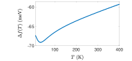
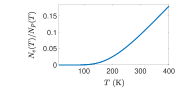
Figure 1: (a) Formation free energy as function of temperature; (b) The ratio of number of electrons ($N_{e}$) to the number of polarons ($N_{P}$) vs. temperature.

Comparing to free electrons in a undeformed lattice, the change in the vibrational entropy $\Delta s_{v}$ per polaron is:

$$\Delta s_{v}=-3\frac{\frac{4}{3}\pi R_{\text{P}}^{3}}{a^{3}}(S_{1}-S_{10}),$$ (8)

where $\frac{4}{3}\pi R_{\text{P}}^{3}/a^{3}$ accounts for the number of the primitive cells occupied by a large polaron, and the factor of 3 represents the three Pb-I stretching modes. If temperature is higher than 50 K, the decrease of the vibrational entropy dominates the change in the translational entropy, cf. Fig.1.

II.3.3 Relative contributions to conductivity from polarons and electrons

The change in entropy $\Delta s$ in forming a polaron is

$$\Delta s=\Delta s_{e}+\Delta s_{v}.$$ (9)

The formation free energy $\Delta f$ per polaron is thus

$$\Delta f(T)=-E_{\text{P}}-T\Delta s,$$ (10)

which is plotted as a function of temperature in Fig.1. The shallow minimum in Fig.1 is due to the larger effective mass $m_{\text{P}}$ of polarons and $n\ll n_{c}$. With the increase of temperature, $|\Delta f(T)|$ is decreased, i.e., polarons become less stable at a higher temperature.

At temperature $T$, the ratio between $N_{e}(T)$ (the number of electrons) and $N_{\text{P}}(T)$ (the number of polarons) is given by Landau and Lifshitz (1980)

$$[\frac{N_{e}(T)}{N_{\text{P}}(T)}]^{2}=e^{2\frac{\Delta f(T)}{k_{B}T}},$$ (11)

where we assume that the formation free energy of hole polarons is the same as that of electron polarons. We can see from Fig.1 that the below 140 K, the number of electrons is negligible. At 300 K, $N_{e}(T)/N_{\text{P}}(T)\thicksim 0.1$. Therefore, the dominant carriers in MAPbI₃ are large polarons, as opposed to electrons and holes.

III dielectric screening

There is a misconception in literature which attributes the temperature dependence of carrier mobility, i.e., $\mu\propto T^{-3/2}$ entirely to the scattering of acoustic phonons. This misconception counters the fact that many non-polar semiconductors do not exhibit the same $T^{-3/2}$ dependence as the perovskite materials although their carriers are scattered primarily by acoustic phonons Zeghbroeck (2011). We believe that the perovskites possess a unique but often overlooked feature, i.e., the existence of a spontaneously polarized phase at low temperatures, which is responsible for the unique temperature dependence of carrier mobility. More specifically, we will reveal in following that it is the temperature dependence of the dielectric function that among other factors, yields the temperature dependence of carrier mobility in the perovskites.

Recent molecular dynamics simulations indicate that there exists a super paraelectric phase in MAPbI₃ below 1000K [Frost et al., 2014a]. It is known that the super paraelectric phase emerges from a spontaneously polarized phase with increased temperature. For ABX₃ perovskites, the critical polarizability $\alpha_{c}$ above which a spontaneous polarization takes place is given by $\alpha_{c}=(a/2)^{3}$/0.383  [Feynman et al., 1977]. For MAPbI₃, $\alpha_{c}=8.16\times 10^{-29}$ m³. On the other hand, the polarizability of MAPbI₃, $\alpha_{\text{dis}}$ is mainly induced by the displacements of Pb²⁺ and I^- ions and can be estimated as $\alpha_{\text{dis}}=2.73\times 10^{-28}$m${}^{3}>\alpha_{c}$ [Zhang et al., 2017]. Hence, below a certain temperature, MAPbI₃ is spontaneously polarized.

For a super paraelectric phase, one can express its dielectric function as follows: Schwinger et al. (1998); Poglitsch and Weber (1987); Feynman et al. (1977); Kittel (1976)

$$\varepsilon(\omega,T)=\varepsilon_{\infty}+\frac{1}{3}\frac{n_{d}p^{2}}{k_{B}T\epsilon_{0}}\frac{1}{1-i\omega\tau(T)}$$ (12)

$$+\frac{9}{\beta(T-\theta)}\frac{\omega_{ip}^{2}}{\omega^{\prime 2}-i\gamma^{\prime}\omega-\omega^{2}}.$$

The first term represents the contribution from the bound electrons at the optical frequencies and room temperature and it is taken from an experimental measurement ($\varepsilon_{\infty}\thickapprox 6.5$) Lin et al. (2015). The second term stems from the rotations of MA ions. The dipole moment of the MA cation is $p=7.64\times 10^{-30}$C$\cdot$m and the number density of the cations is $n_{d}\thickapprox$ $4\times 10^{27}$m^-3 [Frost et al., 2014b]. $\tau(T)$ is the temperature dependent relaxation time of the MA ions Poglitsch and Weber (1987) which is about 0.2 -14 ps Leguy et al. (2015a); Poglitsch and Weber (1987); Wasylishen et al. (1985). The third term represents the contribution of the displacements of Pb²⁺ and I^- ions, and the factor $9/\beta(T-\theta)$ account for the static susceptibility Feynman et al. (1977); Kittel (1987). $\omega_{ip}$ is the frequency of ionic plasmon; $\omega^{\prime}$ and $\gamma^{\prime}$ are the eigenfrequency and friction coefficient of the Pb-I stretching mode Schwinger et al. (1998). $\beta$ is a constant Feynman et al. (1977) with a dimension of inverse temperature (K^-1). It turns out that in MAPbI₃, $\theta\thicksim 0$K is a small number Zhang et al. (2017) compared to $T$. If the spontaneously polarized phase below the critical temperature is ferroelectric, $\theta>0$. If the phase is anti-ferroelectric, $\theta<0$ [Kittel, 1976].

If the frequency $\omega$ is so low ($\omega\ll 7\times 10^{10}$Rad/s) that the product $\omega\tau(T)\ll 1$, $[1-i\omega\tau(T)]^{-1}\thicksim 1$. Hence the second term reduces to $n_{d}p^{2}/(3k_{B}T\epsilon_{0})$. Specifically, at T = 300K and $\omega=0$, the second terms becomes a constant ( 2). Therefore, the second term and the third term scale approximately as $1/T$, and Eq.(12) becomes

$$\varepsilon(\omega,T)=\varepsilon_{\infty}+C(\omega)/T,$$ (13)

where $C(\omega)$ is a materials constant, independent of temperature. This result agree very well with the experimental data at $\omega/2\pi=1$KHz above 160K (cf. Fig. 3 of [Onoda-Yamamuro et al., 1992]) as shown in Fig. 2. Note that this $1/T$ dependence is analogous to Curie-Weiss law due to magnetic phase transitions.

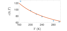
Figure 2: Static dielectric constant as function of temperature in MAPbI₃. The experimental data (squares) are taken from [Onoda-Yamamuro et al., 1992], and the solid line is a fit from Eq. (13).

If $\omega$ is  $7\times 10^{10}-10^{12}$Rad/s, $\omega\tau(T)\thicksim 1$. In this frequency range, the second term becomes a dominant contribution. As a result, $\varepsilon(\omega,T)$ deviates from the $1/T$ behavior, as found experimentally in the case of $\omega/2\pi=90$GHz in [Poglitsch and Weber, 1987].

As will be shown later, the screened polaron-LA phonon interaction is responsible for charge transport in the perovskites. The characteristic acoustic phonon frequency is $\omega_{b}=c_{l}\pi/a$, where $a$ is the lattice constant and $c_{l}$ is the speed of longitudinal sound wave. In MAPbI₃, $\omega_{b}\thicksim 10^{13}$Rad/s [Zhang et al., 2017]. For such a high frequency, $\omega\tau(T)\gg 1$, the second term can be ignored, and Eq.(12) is reduced to Eq.(13) again.

It is experimentally observed that below 150 -160 K, $\varepsilon(\omega,T)$ deviates from the $1/T$ behavior Onoda-Yamamuro et al. (1992), giving rise to contrasting transport behaviors Hutter et al. (2017). This deviation is caused by structural phase transition from tetragonal to orthorhombic phase.

IV charge transport and carrier mobility

IV.1 Polaron-LA phonon vs. polaron-LO phonon interaction

It is generally accepted that as quasiparticles, large polarons result from the interaction between electrons (or holes) with optical phonons in ionic perovskites Zhu and Podzorov (2015); Brenner et al. (2015); Sendner et al. (2016); Menendez-Proupin et al. (2014); Frost et al. (2014a). However, it is often mistakenly assumed that the same optical phonons must also be principally responsible for scatting of the large polarons. This assumption would yield incorrect temperature dependence of carrier mobility, which is the source of confusion and debate in literature Brenner et al. (2015); Zhu and Podzorov (2015); Wright et al. (2016); Sendner et al. (2016). Here we demonstrate that much of the electron-LO phonon interaction $h_{\text{e-LO}}$ is involved in the formation of large polarons, thus the residual interaction $h_{\text{P-LO}}$ is substantially weaker than the interaction between the polaron and the LA phonon, $h_{\text{P-Aph}}$ in MAPbI₃. Based on Born-Huang model of electron-optical phonon interaction, we can show

$$h_{\text{e-LO}}/h_{\text{e-LA}}\thicksim\frac{\frac{3}{2}\hbar\omega_{\text{LO}}(\frac{\hbar}{2m\omega_{\text{LO}}})^{1/4}[4\pi\alpha]^{1/2}}{\frac{1}{\varepsilon}\sqrt{\frac{\hbar}{2M_{j}c_{l}k_{b}}}2\frac{e^{2}}{\epsilon_{0}}n_{\text{cell}}^{1/2}}.$$ (14)

Here $n_{\text{cell}}$ is the number of primitive unit cells in a unit volume. One can see that a softer lattice (smaller sound speed $c_{l}$), larger primitive unit cell (smaller $k_{b}$ and $n_{\text{cell}}$) and smaller $\omega_{\text{LO}}$ will increase the relative importance of $h_{\text{e-LA}}$. Since the electronic part of the polaron wave-function is similar to the free electron wave-function, $h_{\text{P-LA}}\thickapprox h_{\text{e-LA}}$. On the other hand, according to the Feynman model of large polarons,

$$h_{\text{P-LO}}\thicksim(\alpha/10)^{4}h_{\text{e-LO}},$$ (15)

where $\alpha$ is a dimensionless coupling constant Feynman (1955). Combining Eq.(40) to Eq.(15), one has

$$\frac{h_{\text{P-LO}}}{h_{\text{P-LA}}}\thicksim(\alpha/10)^{4}\frac{\frac{3}{2}\hbar\omega_{\text{LO}}(\frac{\hbar}{2m\omega_{\text{LO}}})^{1/4}[4\pi\alpha]^{1/2}}{\frac{1}{\varepsilon}\sqrt{\frac{\hbar}{2M_{j}c_{l}k_{b}}}2\frac{e^{2}}{\epsilon_{0}}n_{\text{cell}}^{1/2}}.$$ (16)

With the material parameters for MAPbI₃, we find $h_{\text{P-LO}}/h_{\text{P-LA}}\thicksim 0.12$. This result is supported by the experiments which reported Wright et al. (2016); Menéndez-Proupin et al. (2015) $h_{\text{P-LO}}/h_{\text{P-LA}}\thicksim$ 0.1. Therefore, the acoustic phonons are chiefly responsible for the scattering while the optical phonons are responsible for the formation of the large polarons in MAPbI₃. Recent experiments also suggest that the e-LO phonon interaction is primarily responsible for the line-width of photoluminescence (PL) spectrum of the perovskites Wright et al. (2016), which is consistent with the preceding analysis. As mentioned earlier, since electrons and holes are stabilized by the interaction with the optical phonons, they have to be “activated” prior to recombination, by absorbing optical phonons. After the annihilation, the optical phonons have to be emitted to restore the deformed lattice. The energy of the absorbed and emitted phonons is responsible for the PL line-width.

IV.2 Scattering mechanisms

The Hamiltonian of the system can be written as

$$H=K_{\text{P}}+H_{\text{PP}}+H_{\text{P-def}}+H_{\text{P-LA}}+H_{\text{LA}},$$ (17)

where $K_{\text{P}}$ denotes the sum of single polaron Hamiltonians, and $H_{\text{PP}}$ is the Coulomb interaction between the polarons. $H_{\text{P-def}}$ represents the interaction between the polarons and defects whereas $H_{\text{P-LA}}$ is the interaction between the polarons and longitudinal acoustic (LA) phonons; $H_{\text{LA}}$ is the Hamiltonian of LA phonons. The interaction between the polarons and transverse phonons, and the residual interaction between the polarons and LO phonons are small, and can be neglected. Note that $H_{\text{PP}}$, $H_{\text{P-def}}$ and $H_{\text{P-LA}}$ represent dressed or effective interactions and are related to the corresponding bare interactions via the dielectric function, e.g., $H_{\text{PP}}=H_{\text{PP}}^{\text{bare}}/\varepsilon(\omega,T)$.

We next apply the Boltzmann equation to elucidate the transport behavior of large polarons in the perovskites. The key physical quantity of interest is distribution function of the polarons, whose temporal rate change is given by total collision frequency $\nu_{t}$, including scattering contributions of polaron-polaron, polaron-defect and polaron-LA phonon. $\nu_{t}$ is related to the charge carrier mobility $\mu$ by $\mu=e/m_{\text{P}}\nu_{t}$. We show that the large polarons are stable against the three collision processes in Supporting Information and to a good approximation, we can describe the translational motion of the polarons by plane-waves. Thus the energy of the polaron is given as $\varepsilon_{\mathbf{p}}=\mathbf{p}^{2}/2m_{\text{P}}$, where $\mathbf{p}$ is the plane-wave momentum. We denote the non-equilibrium distribution function of polarons in state $|\mathbf{p}\rangle$ as $f_{\mathbf{p}}(t)$, and the distribution function of the LA phonons as $N_{\mathbf{k}}(t)$ ($\mathbf{k}$ is the wave vector of the phonons) and their corresponding equilibrium counterparts are given as $f_{0}$ and $N_{0}$.

The change rate of $f_{\mathbf{p}}(t)$ due to the polaron and LA phonon collision is given by $\nu_{\text{P-LA}}=(\partial f_{\mathbf{p}}/\partial t)_{\text{P-LA}}$ and is calculated in the following.

$$(\frac{\partial f_{\mathbf{p}}}{\partial t})_{\text{P-LA}}=-\sum_{\mathbf{k}}\frac{\partial N_{0}(\omega_{\mathbf{k}})}{\partial\hbar\omega_{\mathbf{k}}}[f_{0}(\mathbf{p}^{\prime})-f_{0}(\mathbf{p})]$$ (18)

$$\{w(\mathbf{p}^{\prime},\mathbf{k};\mathbf{p})(\varphi_{\mathbf{p}^{\prime}}-\varphi_{\mathbf{p}}+\chi_{\mathbf{k}})\delta(\varepsilon_{\mathbf{p}}-\varepsilon_{\mathbf{p}^{\prime}}-\hbar\omega_{\mathbf{k}})$$

$$-w(\mathbf{p}^{\prime};\mathbf{p},\mathbf{k})(\varphi_{\mathbf{p}^{\prime}}-\varphi_{\mathbf{p}}-\chi_{\mathbf{k}})\delta(\varepsilon_{\mathbf{p}}-\varepsilon_{\mathbf{p}^{\prime}}+\hbar\omega_{\mathbf{k}})\}.$$

Here $\varphi$ and $\chi$ describe the deviations of $f_{\mathbf{p}}$ and $N_{\mathbf{k}}$ from their equilibrium values: $f_{\mathbf{p}}-f_{0}(\varepsilon)=-\varphi\partial f_{0}(\varepsilon)/\partial\varepsilon$, and $N_{\mathbf{k}}-N_{0}(\mathbf{k})=-\chi\partial N_{0}(\omega_{\mathbf{k}})/\partial\hbar\omega_{\mathbf{k}}$. $w(\mathbf{p}^{\prime},\mathbf{k};\mathbf{p})$ is the probability amplitude defined as $w(\mathbf{p}^{\prime},\mathbf{k};\mathbf{p})(N_{\mathbf{k}}+1)=2\pi|\langle\mathbf{p}^{\prime},\mathbf{k}|H_{\text{P-LA}}($emission$)|\mathbf{p}\rangle|^{2}/\hbar$, $w(\mathbf{p}^{\prime};\mathbf{p},\mathbf{k})$ is defined by $w(\mathbf{p}^{\prime};\mathbf{p},\mathbf{k})N_{\mathbf{k}}=2\pi|\langle\mathbf{p}^{\prime}|H_{\text{P-LA}}($absorption$)|\mathbf{p},\mathbf{k}\rangle|^{2}/\hbar$ [Lifshitz and Pitaevskii, 1981]. Similar rate equations can be obtained for $\nu_{\text{P-def}}$ and $\nu_{\text{PP}}$ and their expressions are given in Supporting Information.

The characteristic frequency of the LA phonons is $\omega_{b}=c_{s}k_{b}$, where $c_{s}$ is the average sound speed in the longitudinal direction. $k_{b}=\pi/a$ is the wave-vector at the Brillouin zone boundary Callaway (2013). Because the elastic constants of the perovskites are relatively small, $c_{s}$ and $\omega_{b}$ are also small. In the tetragonal phase He and Galli (2014); Qian et al. (2016) of MAPbI₃, $c_{s}\approx$ 2147 m/s, and $\omega_{b}\sim$ 82 K. In the pseudo-cubic phase He and Galli (2014); Qian et al. (2016), $c_{s}\approx 2824$ m/s, $\omega_{b}\thicksim$ 107 K. Thus at room temperature, $k_{B}T\gtrsim\hbar\omega_{b}$ and the LA phonons are fully excited Hutter et al. (2017). These fully excited LA phonons increase the P-LA scattering probability and are principally responsible for polaron scattering. In addition, the phonon distribution function $N_{0}(\omega_{\mathbf{k}})$ in Eq. (53) can be reduced to $N_{0}(\omega_{\mathbf{k}})\thickapprox k_{B}T/\hbar\omega_{\mathbf{k}}$.

We can now derive an analytical expression for the change rates $\partial f_{\mathbf{p}}/\partial t$ induced by the three collision processes $H_{\text{PP}}$, $H_{\text{P-def}}$ and $H_{\text{P-LA}}$. More specifically, change rate due to the polaron-polaron scattering is given by Peierls (2001); Zhang et al. (2017) $\nu_{\text{PP}}=(\partial f_{\mathbf{p}}/\partial t)_{\text{PP}}$:

$$\nu_{\text{PP}}\thicksim\left[\frac{T}{300\varepsilon_{s1}+(T-300)\varepsilon_{\infty}}\right]^{2}n$$ (19)

$$\frac{4\pi^{3/2}\hbar^{3}e^{-3/2}}{(2m_{\text{P}}k_{B}T)^{3/2}}\frac{1}{\hbar}\frac{d^{4}}{a^{6}}(\frac{e^{2}}{\epsilon_{0}})^{2}\frac{(kT)^{2}}{D^{3}},$$

where the dielectric function $\varepsilon_{s1}=\varepsilon(\omega_{b},300)$; $D\thicksim$ 3 eV is the conduction band width Brivio et al. (2014); Umari et al. (2014); Menendez-Proupin et al. (2014) of MAPbI₃ and $d=2R_{\text{P}}$ is the diameter of the polaron. The change rate due to the polaron-defect scattering is Lifshitz and Pitaevskii (1981); Callaway (2013); Zhang et al. (2017) given by $\nu_{\text{P-def}}=(\partial f_{\mathbf{p}}/\partial t)_{\text{P-def}}$ :

$$\nu_{\text{P-def}}\thicksim\left[\frac{T}{300\varepsilon_{s1}+(T-300)\varepsilon_{\infty}}\right]^{2}C\frac{2\pi}{\hbar}$$ (20)

$$\left(\frac{e^{2}\Delta z}{\epsilon_{0}}\right)^{2}\frac{1}{D^{2}a^{3}}\frac{\hbar^{4}}{(2m_{\text{P}}k_{B}T)^{2}}k_{B}T,$$

where $C$ is the number of defects per cubic meter and $\Delta z$ is the effective charge of the defect. The change rate due to polaron and LA phonon scattering is given by $\nu_{\text{P-LA}}=(\partial f_{\mathbf{p}}/\partial t)_{\text{P-LA}}$:

$$\nu_{\text{P-LA}}\thicksim\left[\frac{T}{300\varepsilon_{s1}+(T-300)\varepsilon_{\infty}}\right]^{2}\frac{\pi}{M\omega_{b}k_{b}^{2}a^{3}}$$

$$\frac{4\pi}{3}k_{b}^{3}(\frac{ze^{2}}{\epsilon_{0}})^{2}(\frac{k_{B}T}{\hbar\omega_{b}})^{2}n\frac{4\pi^{3/2}\hbar^{3}e^{-3/2}}{(2m_{\text{P}})^{3/2}(k_{B}T)^{5/2}},$$ (21)

where $z$ is the weighted nuclear charges of the ions and $M$ is the reduced mass of Pb and I ions.

It is known that dominant defects in halide perovskites are not particularly harmful to charge transport because they do not create detrimental deep levels within the band gap Yin et al. (2015, 2014); Miller (2014). Therefore, in our model, only shallow defects are considered, which could induce lattice deformation and charge states at the defect center. Because polaron scattering due to the former is much smaller than the latter, we can approximate $H_{\text{P-def}}$ by Coulomb interaction between the point charges at the defect center and the polarons.

To compare the relative importance of the scattering processes, we evaluate the three terms by taking I^- vacancies as an example of defects in MAPbI₃. We assume a moderate defect concentration at $C=4.0\times 10^{20}$cm^-3 and $\Delta z=1.22$. The consideration of other point defects will only change $\Delta z$ by a small amount ($\Delta$z = 1 - 3). The three contributions as a function of temperature are plotted in Fig. 8. We find that at room temperature $\nu_{\text{P-Aph}}\gg\nu_{\text{P-def}}\gg\nu_{\text{PP}}$. Therefore, the polaron-LA phonon scattering dominates charge transport in MAPbI₃, and $\mu$ would appear insensitive to the defects.

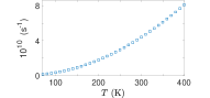
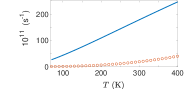
Figure 3: (a) The polaron-polaron collision frequency as a function of $T$ determined by Eq.(49); (b) The polaron-I^- vacancy collision frequency (circles) and the polaron-LA phonon collision frequency (solid line) as functions of T determined by Eq. (52) and (61). $\varepsilon_{0}=70$ and $\varepsilon_{\infty}=6.5$ [Lin et al., 2015] are used in the plot.

IV.3 Concentration dependence of mobility

If we ignore $\nu_{\text{P-def}}$ and $\nu_{\text{PP}}$, we arrive at the key result of the model:

$$\mu\varpropto n^{-1}m_{\text{P}}^{1/2}T^{-3/2}.$$ (22)

First, we find that the mobility is inversely proportional to the carrier concentration $n$, and this finding is consistent to the experimental measurements Bi et al. (2014) in p-doped MAPbI₃. In Fig. 4, we compare the experimental hole mobility $\mu_{h}$ (squares) with the theoretical values (solid line) as a function of $n^{-1}$ where a good agreement is found.

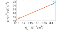
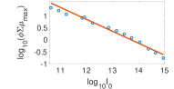
Figure 4: (a) Hole mobility $\mu$ vs. $n^{-1}_{h}$ for p-doped MAPbI₃. The experimental data (squares) are taken from [Bi et al., 2014]; the solid line is a fit of Eq. (22). (b) The logarithm of the effective carrier mobility, log${}_{10}\phi\Sigma\mu$ is plotted as a function of the logarithm of incident photon flux, log${}_{10}I_{0}$. The experimental data (circles) are taken from [Oga et al., 2014], and the solid line is a fit of Eq. (23).

Let $\gamma$ be the electron-hole recombination coefficient, $\kappa$ the generation probability per impinging photon and $G$ the volume density of photons in the sample, we can express $n=(\gamma^{-1}\kappa G)^{1/2}$ by assuming $n$ is much larger than the trap center concentration. Here, $G=I_{0}/l_{\text{abs}}$, $I_{0}$ is the incident photon flux and $l_{\text{abs}}$ is the absorption length Chen et al. (2016). Substitute the expression of $n$ into Eq. (22), one obtains:

$$\mu\varpropto(l_{\text{abs}}\gamma)^{1/2}(\kappa I_{0})^{-1/2}T^{-3/2}.$$ (23)

The circles in Fig. 4 are experimental data Oga et al. (2014) for effective mobility $\phi\mu$ vs. incident flux $I_{0}$, and the solid line is a fit based on Eq. (23). Here we have to adjust the intercept due to a lack of experimental values of $\kappa$, $l_{\text{abs}}$ and $\gamma$ in [Oga et al., 2014], nevertheless the agreement in the slope between the theory and the experiment is very good.

IV.4 Temperature dependence of mobility

Finally, we compare the theoretical prediction with experimental data on carrier mobility as a function of temperature making use of Eq. (61) and $\mu(T)=e/m_{\text{P}}\nu_{\text{P-LA}}$. Because the values of $\varepsilon_{0}$, $\varepsilon_{\infty}$ and $n$ are not available in the experiments Milot et al. (2015); Savenije et al. (2014), we have to use $n$ as a fitting parameter in the comparison. By taking $\varepsilon_{\infty}$ = 4.5 and $\varepsilon_{0}$ = 24.5 from first-principles calculations Frost et al. (2014a); Brivio et al. (2014), we can fit the theoretical mobility to the experimental data in Fig. 5. For the first experiment Milot et al. (2015), $n=2.3\times 10^{17}$cm^-1 was used in the fitting while for the second experiment Savenije et al. (2014), $n=8.3\times 10^{17}$cm^-1 was used in the fitting. Both values of $n$ are reasonable Chen et al. (2016) and for both cases, satisfactory agreements to the experimental data are obtained.

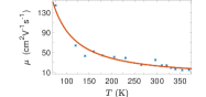
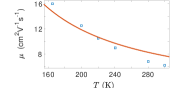
Figure 5: The carrier mobility $\mu$ as a function of temperature. The solid curves are obtained from Eq. (61) with fitting a parameter of $n$. (a) The experimental data (crosses) is from [Milot et al., 2015], and $n=2.3\times 10^{17}$cm^-3. (b) The experimental data (squares) is from Savenije et al., 2014, and $n=8.3\times 10^{17}$cm^-3.

In a recent experiment by Hutter et al., the temperature dependence of carrier mobility in MAPbI₃ was shown to exhibit two regimes of contrasting behaviors Hutter et al. (2017). Above 150 K, carrier mobility $\mu(T)\varpropto T^{-3/2}$ while below 150 K, the mobility drops precipitately, decreasing with decreased temperature. Using the experimental dielectric function $\varepsilon(\omega,T)$ for $\omega/2\pi=1$KHz as obtained in Onoda-Yamamuro et al. (1992), our analytical expression in Eq. (61) can reproduce the experimental data of Hutter reasonably well in both regimes, as shown in Fig.6. In the tetragonal phase ($T>$ 150 K), the mobility behaves as $\mu(T)\varpropto T^{-3/2}$, while in the orthorhombic phase ($T<$ 150K), the mobility decreases with decreasing temperature with a sharp drop around 150 K. We further speculate that the reason that the earlier experiments observed only the regime of $\mu(T)\varpropto T^{-3/2}$ is due to the presence Kong et al. (2015); Hutter et al. (2017) of the tetragonal phase at $T<$ 150 K.

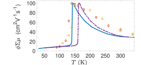
Figure 6: Product of generation yield $\phi$ and mobility $\Sigma\mu$ as function of temperature. Circles (diamonds) are measured during the heating (cooling) process [Hutter et al., 2017]. The dash line is calculated from the experimental dielectric function [Onoda-Yamamuro et al., 1992] and the solid line is obtained by shifting the the tetragonal-orthorhombic transition temperature from [Onoda-Yamamuro et al., 1992] to [Hutter et al., 2017].

V Summary

In conclusion, we proposed a theoretical model that can elucidate key experimental observations on charge transport in hybrid perovskite materials. Essential to the model is improved understanding crucial to charge transport, including that the acoustic phonons as opposed to the optical phonons are responsible for the scattering of large polarons, the acoustic phonons are fully excited due to the “softness”of the perovskites, and the temperature dependent dielectric function is the key contributor to the temperature dependence of the mobility. Analytic expressions were given for various contributions to the carrier mobility and compared to the experimental measurements with good agreements. By directly relating the carrier mobility to material parameters, the present work may provide guidance for materials design and form a starting point for more rigorous first-principles predictions of transport properties.

The work at California State University Northridge was supported by NSF-PREM program via grant DMR-1205734. Discussion with Guangjun Nan is acknowledged. The authors wish to thank anonymous referees for their stimulating comments.
^†haiqing0@csrc.ac.cn, ^∗ganglu@csun.edu

Supplemental Material for

Charge Transport in Hybrid Halide Perovskites
Mingliang Zhang^1,2, Xu Zhang², Ling-Yi Huang², Hai-Qing Lin¹ and Gang Lu^2
1Beijing Computational Science Research Center, Beijing 100193, China
²Department of Physics and Astronomy, California State University Northridge, Northridge, CA 91330, USA

V.1 dielectric screening

In MAPbI₃, there are four factors contributing to dielectric function $\varepsilon(\omega,T)$: (i) bound electrons; (ii) the displacements of Pb²⁺ and I^- ions of the lattice frame; (iii) the rotation of MA dipoles and (iv) free electrons. The contribution (iv) of ‘free’ carriers is negligible. We will see that the displacements of ions is the most important.

V.1.1 MA dipoles

Let us show that the MA dipoles cannot form a spontaneous polarized phase. Both experiments Leguy et al. (2015a) and simulations Brivio et al. (2013); Mosconi et al. (2014); Quarti et al. (2015) show that the rotational barrier for the changing direction of a MA dipole is larger than 13.5meV (157K): below 157K, the MA dipoles are locked in various orientations, i.e. a spontaneous polarization cannot be implemented by the MA dipoles below 157K. In addition, the attraction energy between two dipoles is the strongest if they take the same direction and are parallel to the connection line of their centers Schwinger et al. (1998):

$$U=-\frac{2}{4\pi\epsilon_{0}\varepsilon_{\infty}}\frac{p_{1}p_{2}}{|\mathbf{x}_{1}-\mathbf{x}_{2}|^{3}},$$ (24)

where $\mathbf{x}_{1}$ and $\mathbf{x}_{2}$ are the position vectors of two dipoles $\mathbf{p}_{1}$ and $\mathbf{p}_{2}$. In MAPbI₃, the nearest distance between two MA dipoles is $|\mathbf{x}_{1}-\mathbf{x}_{2}|=6.3$Å, $\varepsilon_{\infty}=6.5$ [Lin et al., 2015], the dipole moment of MA⁺ is Frost et al. (2014b) $p=7.64\times 10^{-30}$C$\cdot$m, then $U=4$meV=47K$\ll$25meV=300K. At $T>47$K, the MA dipoles cannot align in the same direction to form a ferroelectric. Therefore, only the wobbling and rotating of the MA dipoles contribute to the dielectric polarization.

V.1.2 Spontaneous polarization at low temperature

We give a simple reasoning to support that the existence of a spontaneously polarized phase at low temperature is caused by the displacements of Pb²⁺ and I^- ions. The perovskite crystal can be viewed as composed of three types of chains: (1) —I^-—Pb²⁺—I^-—; (2) —I^-—I^-—; and (3) —MA—MA—. Denote the lattice constant of MAPbI₃ as $a$, the distance between two MAs is $a$, the distance between two I^- ions is $a$, the distance between I^- and Pb²⁺ is $a/2$. If one applies an electric field along the direction of these chains, ions will move accordingly. Since the field produced by a dipole is proportional to the inverse cube of distance, in a processes of spontaneous polarization, we may ignore the—I^-—I^-— chains and the —MA—MA— chains. For an ion in a given chain, the field at the position of that ion produced by other —I^-—Pb²⁺—I^-— chains is much weaker than the field produced by the ions in the same chain Feynman et al. (1977). Thus we only need to consider one —I^-—Pb²⁺—I^-— chain. In a perovskite structure, the critical polarizability $\alpha_{c}$ for the existence of a spontaneously polarized (ferroelectric or anti-ferroelectric) phase is Feynman et al. (1977): $\alpha_{c}=(a/2)^{3}/0.383$. In MAPbI₃, $a=6.3$Å, then $\alpha_{c}=8.16\times 10^{-29}$m³.

The electronic polarization of I^- and Pb²⁺ ions, and the orientation polarization of the MA dipoles are not enough to produce a spontaneous polarization. The polarizabilities of I^- and Pb²⁺ are $\alpha_{\text{I}^{-}}=6.43\times 10^{-30}$m³, $\alpha_{\text{Pb}^{2+}}=4.9\times 10^{-30}$m³Tessman et al. (1953), which are far from enough to produce a spontaneous polarization. If the MA dipole can rotate freely, the average dipole $\langle p\rangle_{T}$ at temperature $T$ is Schwinger et al. (1998)

$$\langle p\rangle_{T}\thickapprox\frac{p^{2}}{3k_{B}T\epsilon_{0}}\epsilon_{0}E,$$ (25)

where $E$ is the strength of electric field. Then the rotational polarizability $\alpha_{\text{MA}}$ of MA dipoles is

$$\alpha_{\text{MA}}=\frac{p^{2}}{3k_{B}T\epsilon_{0}}.$$ (26)

One can see that when $T\lesssim 44$K, $\alpha_{\text{MA}}$ could reach $\alpha_{c}$. However, we overestimated $\alpha_{\text{MA}}$. In the fabrication process, the orientations of MA dipoles are random. The energy barrier for the reorientation of a MA dipole is at least 13.5 meV (157.2K) Frost et al. (2014b); Leguy et al. (2015b). When the temperature is lowered to $T\lesssim 44$K, the MA dipoles are already locked into various orientations by the energy barrier. A spontaneous polarization cannot be produced from the reorientation of the MA dipoles.

Let us consider the induced dipole caused by the displacements of Pb²⁺ and I^- ions. To make Pb²⁺ sit in the octahedral hole of I^-, one requires that $0.414R<r<0.732R$ [HomePage, 2016], where $r=1.33$Å is the radius of Pb²⁺, $R=2.06$Å is the radius of I^- [Wikipedia, 2016]. One can see $r/R=0.65$, Pb²⁺ is not enclosed by the I^- ions too tightly. Denote the spring constant of Pb²⁺—I^- as $k$, the charge of I^- as $q_{\text{I}^{-}}$, the charge of Pb²⁺ as $q_{\text{Pb}^{2+}}$. The stretch frequency of Pb²⁺—I^- is $\widetilde{\nu}=$106.9 cm^-1 [Juarez-Perez et al., 2014]. Then $k=m_{r}\omega^{2}\thicksim 53$Nm^-1, where $m_{r}$ is the reduced mass of Pb²⁺ and I^-. In an electric field $\mathbf{E}$, the induced dipole $\mathbf{p}_{in}=q_{\text{Pb}^{2+}}d_{2}+q_{\text{I}^{-}}d_{1}$ of —Pb²⁺—I^-—  is

$$\mathbf{p}_{in}=\frac{q_{\text{Pb}^{2+}}^{2}+q_{\text{I}^{-}}^{2}}{k\epsilon_{0}}\epsilon_{0}E,$$ (27)

where $d_{1}$ and $d_{2}$ are the induced displacements of I^- ion and Pb²⁺ ion. The polarizability $\alpha_{\text{dis}}$ due to the displacements of Pb²⁺ and I^- ions is

$$\alpha_{\text{dis}}=\frac{q_{\text{I}^{-}}^{2}+q_{\text{Pb}^{2+}}^{2}}{\epsilon_{0}k}\thickapprox 2.73\times 10^{-28}\text{m}^{3}>\alpha_{c}.$$ (28)

Above estimation only considered the induced displacements of Pb²⁺ and I^- ions without the perturbation of thermal vibrations. Considering $\alpha_{\text{dis}}$ is only three times larger than $\alpha_{c}$, thermal vibrations could significantly reduce $d_{1}$ and $d_{2}$, i.e $\alpha_{\text{dis}}$. It seems reasonable to assume that at a low enough temperature, MAPbI₃ is in a spontaneously polarized phase (either in a ferroelectric phase or in an anti-ferroelectric phase). To decide if a ferroelectric or an anti-ferroelectric is more favorable, one needs a more refined calculation to determine the direction of the internal field on the —I^-—I^-— chain is whether parallel or antiparallel to the field on the —I^-—Pb²⁺—I^-— chain.

V.1.3 Neglect of the susceptibility from free carriers

The screening caused by the ‘free’ carriers may affect the properties of ABX₃ in two aspects: (a) screening the the electric field $E_{\text{pol}}$ which causes spontaneous polarization; (b) screening three bare interactions: polaron-polaron (PP) interaction, polaron-defect interaction (P-def), and polaron-acoustic phonon interaction (P-LA) Pines and Nozieres (1966).

Let us first discuss effect (a). The maximal screening is reached if the positive and negative charges are concentrated in two opposite surfaces. The observed size $l$ of a ferroelectric domain is $l\lesssim 10^{-6}$m Kutes et al. (2014); Fan et al. (2015); Kim et al. (2015), then the surface charge density $\sigma$ is $\sigma\thicksim nel$. The electric field $E_{\text{res}}$ produced by the free carriers is $E_{\text{res}}\thicksim nel/\epsilon_{0}$. The induced dipole $p_{\text{res}}$ by the field $E_{\text{res}}$ of free carriers is $p_{\text{res}}\thicksim\alpha_{\text{cri}}nle$. If $p_{\text{res}}$ is comparable to the dipole $p($MA$)$ of MA, then the spontaneous polarization is modified. For $l=10^{-6}$m, the upper limit concentration is $n^{\text{upper}}=p($MA$)/\alpha_{\text{cri}}le\thicksim 5.85\times 10^{17}$cm^-3. Considering we used the largest $l$, the actual $n^{\text{upper}}$ may be higher than above value. Then, for $n_{e}<10^{18}$cm^-3, the changes in elastic constants and $E_{\text{pol}}$ are negligible. ABX₃ is still in a super paraelectric phase.

Secondly, let us discuss effect (b). For $2\times 10^{17}\lesssim n_{e}\lesssim 10^{18}$cm^-3 and $T\lesssim$350K the Debye-Huckel screening length $r_{\text{DH}}$ is $r_{\text{DH}}=\sqrt{\epsilon_{0}k_{B}T/ne^{2}}\lesssim 28.9$Å. The diameter of an EP is $2R_{\text{EP}}$ $\thicksim 56.7$Å $\gtrsim$ $r_{DH}$. Debye-Huckel type electronic screening does not happen; for $n_{e}<2\times 10^{17}$cm^-3 and $T>350$K, $r_{\text{DH}}^{-1}=(ne^{2}/\epsilon_{0}k_{B}T)^{1/2}\ll k_{b}$, the Debye-Huckel screening plays little role except for the phonons with very low frequencies Ziman (1972). But if $n>10^{18}$cm^-3, the carriers are electrons (holes), the Thomas-Fermi screening caused by the ‘free’ electrons.is significant.

In summary, if $I_{0}$ is not too big, i.e. $n_{e}<10^{18}$cm^-3, the screening mainly comes from the bound electrons and the displacements of ions.

V.2 Screened interactions

The effective interaction $H_{\text{e-LA}}$ of electron-LA phonon relates to the bare interaction by Pines and Nozieres (1966):

$$H_{\text{e-LA}}=H_{\text{e-LA}}^{\text{bare}}/\varepsilon(\omega,T).$$ (29)

To get a manageable expression for mobility $\mu$, we use

$$\varepsilon(\omega_{b},T)=\varepsilon_{\infty}+\frac{C(\omega_{b})}{T},$$ (30)

at the characteristic frequency $\omega_{b}=c_{s}k_{b}\thicksim 1.41\times 10^{13}$rad/s of P-Aph interaction to all frequency $\omega$. Denote $\varepsilon_{s1}=\varepsilon(\omega_{b},T_{1})$ at a specific temperature $T_{1}$, then for temperature $T$, one has

$$\frac{1}{\varepsilon(\omega_{b},T)}=\frac{T}{T_{1}\varepsilon_{s1}+(T-T_{1})\varepsilon_{\infty}}\thickapprox\frac{T}{T_{1}\varepsilon_{s1}}.$$ (31)

The last step of Eq.(31) results from $\varepsilon_{s1}\gg\varepsilon_{\infty}$ at all temperature. Unfortunately, no $\varepsilon(\omega,T)$ data around $\omega_{b\text{ }}$are reported in this frequency range Lin et al. (2015). Taking $T_{1}=$300K is convenient. Using the static dielectric constant $\varepsilon_{0}\thickapprox 70$ at $T_{1}=300$K Lin et al. (2015), then $\varepsilon_{s1}\thicksim(\varepsilon_{\infty}+\varepsilon_{0})/2\thicksim 38$, which is close to the interpolated value from lower and higher frequencies, cf. Fig.2b of Lin et al. (2015). For $\varepsilon_{\infty}=6.8,$ $\varepsilon_{0}=30$ Bokdam et al. (2016), $\varepsilon_{s1}\thicksim(\varepsilon_{\infty}+\varepsilon_{0})/2\thicksim 18$, which is quite close to Re$\varepsilon(9$meV$)=20$ directly calculated from DFPT Bokdam et al. (2016). Similarly, for $\varepsilon_{\infty}=4.5,$ $\varepsilon_{0}=24.1$ Brivio et al. (2014), $\varepsilon_{s1}\thicksim(\varepsilon_{\infty}+\varepsilon_{0})/2\thicksim 15$. As noticed in Sec.V.1.3, Eq.(31) are applicable for $n_{e}<10^{18}$cm^-3. The effective interaction $H_{\text{int}}$ relates to the bare interaction $H_{\text{int}}^{\text{bare}}$ by $H_{\text{int}}=H_{\text{int}}^{\text{bare}}/\varepsilon(\omega_{b},T)$, where $H_{\text{int}}^{\text{bare}}$ represents any of $H_{\text{ee}}^{\text{bare}}$, $H_{\text{e-def}}^{\text{bare}}$ and $H_{\text{e-LA}}^{\text{bare}}$. Then,

$$h_{\text{ee}}=\frac{e^{2}}{\epsilon_{0}\mathcal{V}|\mathbf{k}_{2}-\mathbf{k}_{2}^{\prime}|^{2}\varepsilon},$$ (32)

where $\varepsilon^{-1}$ is given by Eq.(31). The effective ee interaction for whole sample is $H_{\text{ee}}=\sum_{j<k}h_{\text{ee}}(j,k)$. Similarly,

$$h_{\text{e-def}}=\frac{1}{4\pi\epsilon_{0}}\frac{\Delta z_{\text{I}^{-}}e^{2}}{\varepsilon R_{\text{e-V(I}^{-}\text{)}}},$$ (33)

the e-def interaction for whole sample is $H_{\text{e-def}}=\sum_{j\beta}h_{\text{e-def}}(j,\beta)$.

V.3 $h_{\text{P-LO}}$ and $h_{\text{P-LA}}$

The bare interaction of an electron with wave vector $\mathbf{k}_{i}$ with LA phonons can be written as

$$h_{\text{e-LA}}^{\text{bare}}=-i\sum_{j\mathbf{Kk}}\frac{1}{\varepsilon}\sqrt{\frac{\hbar\mathcal{N}}{2M_{j}\omega_{\text{LA}}(\mathbf{k})}}\mathbf{e}_{j}^{(\text{LA})}(\mathbf{k})\cdot(\mathbf{k}+\mathbf{K})$$

$$V_{j\mathbf{k}+\mathbf{K}}c_{\mathbf{k}_{i}+\mathbf{k}+\mathbf{K}}^{{\dagger}}c_{\mathbf{k}_{i}}(a_{\mathbf{k}\text{LA}}+a_{-\mathbf{k}\text{LA}}^{{\dagger}}),$$ (34)

where $\omega_{\text{LA}}(\mathbf{k})=c_{l}k$, $c_{l}$ is the speed of longitudinal sound wave. For a normal process ($\mathbf{K}=0$), one may estimate Eq.(34) by

$$h_{\text{e-LA}}^{\text{bare}}\thicksim\sum_{j\mathbf{k}}\sqrt{\frac{\hbar\mathcal{N}}{2M_{j}c_{l}k}}k\frac{e^{2}}{\epsilon_{0}k^{2}\mathcal{V}}.$$ (35)

Then the screened interaction is

$$h_{\text{e-LA}}\thicksim\sum_{\mathbf{k}}\frac{1}{\varepsilon(c_{l}k,T)}\sqrt{\frac{\hbar\mathcal{N}}{2M_{j}c_{l}k}}k\frac{e^{2}}{\epsilon_{0}k^{2}\mathcal{V}}.$$ (36)

To simplify Eq.(35), let us consider

$$\langle\frac{1}{k^{3/2}}\rangle=\frac{\int_{0}^{k_{b}}\frac{1}{k^{3/2}}4\pi k^{2}dk}{\int_{0}^{k_{b}}4\pi k^{2}dk}=\frac{2}{k_{b}^{3/2}},$$

then

$$\sum_{\mathbf{k}}\frac{1}{k^{3/2}}=\frac{\mathcal{V}\frac{4\pi}{3}k_{b}^{3}}{(2\pi)^{3}}\langle\frac{1}{k^{3/2}}\rangle=\frac{\mathcal{V}\frac{4\pi}{3}k_{b}^{3}}{(2\pi)^{3}}\frac{2}{k_{b}^{3/2}}.$$

Eq.(35) becomes:

$$h_{\text{e-LA}}^{\text{bare}}\thicksim\frac{\mathcal{V}\frac{4\pi}{3}k_{b}^{3}}{(2\pi)^{3}}\sqrt{\frac{\hbar\mathcal{N}}{2M_{j}c_{l}k_{b}}}2k_{b}^{-1}\frac{e^{2}}{\epsilon_{0}\mathcal{V}}.$$

The interaction between an electron and LO phonons is Kittel (1987)

$$h_{\text{e-LO}}=\sum_{\mathbf{q}}(V_{\mathbf{q}}a_{\mathbf{q}}e^{i\mathbf{q}\cdot\mathbf{r}}+V_{\mathbf{q}}^{{\dagger}}a_{\mathbf{q}}^{{\dagger}}e^{-i\mathbf{q}\cdot\mathbf{r}}).$$ (37)

The order of magnitude of Eq.(37) is

$$h_{\text{e-LO}}\thicksim\sum_{\mathbf{q}}i\hbar\omega_{\text{LO}}\frac{1}{q\mathcal{V}^{1/2}}(\frac{\hbar}{2m\omega_{L}})^{1/4}[4\pi\alpha]^{1/2},$$ (38)

where

$$\alpha=\frac{e^{2}}{4\pi\epsilon_{0}(2\hbar\omega_{\text{LO}})}(\frac{2m\omega_{L}}{\hbar})^{1/2}(\frac{1}{\varepsilon_{\infty}}-\frac{1}{\varepsilon_{0}}).$$ (39)

To further simplify Eq.(38), let us consider

$$\langle\frac{1}{q}\rangle=\frac{\int_{0}^{k_{b}}\frac{1}{q}4\pi q^{2}dq}{\int_{0}^{k_{b}}4\pi q^{2}dq}=\frac{3}{2k_{b}},$$

then

$$\sum_{\mathbf{q}}\frac{1}{q}=\frac{\mathcal{V}\frac{4\pi}{3}k_{b}^{3}}{(2\pi)^{3}}\langle\frac{1}{q}\rangle=\frac{\mathcal{V}\frac{4\pi}{3}k_{b}^{3}}{(2\pi)^{3}}\frac{3}{2k_{b}}.$$

Eq.(38) becomes

$$h_{\text{e-LO}}\thicksim\frac{\mathcal{V}\frac{4\pi}{3}k_{b}^{3}}{(2\pi)^{3}}\frac{3}{2k_{b}}\hbar\omega_{\text{LO}}\frac{1}{\mathcal{V}^{1/2}}(\frac{\hbar}{2m\omega_{L}})^{1/4}[4\pi\alpha]^{1/2}.$$

Using $\mathcal{N}=n_{\text{cell}}\mathcal{V}$, where $n_{\text{cell}}$ is the number of primitive cells in unit volume. One has

$$h_{\text{e-LO}}/h_{\text{e-LA}}\thicksim\frac{\frac{3}{2}\hbar\omega_{\text{LO}}(\frac{\hbar}{2m\omega_{L}})^{1/4}[4\pi\alpha]^{1/2}}{\frac{1}{\varepsilon}\sqrt{\frac{\hbar}{2M_{j}c_{l}k_{b}}}2\frac{e^{2}}{\epsilon_{0}}n_{\text{cell}}^{1/2}},$$ (40)

where $\varepsilon^{-1}$ is given by Eq.(31). According to the polaron theory Feynman (1955), the interaction between polaon and LO phonons (the residual e-LO interaction) is small: $h_{\text{P-LO}}/h_{\text{e-LO}}\thicksim(\alpha/10)^{4}$, where $\alpha$ is the dimensionless coupling constant given by Eq.(39). On the other hand, $h_{\text{P-Aph}}\thickapprox h_{\text{e-LA}}$. Finally,

$$h_{\text{P-LO}}/h_{\text{P-LA}}\thicksim(\alpha/10)^{4}h_{\text{e-LO}}/h_{\text{e-LA}}\thicksim 0.12.$$ (41)

If one use line width as an indication of the strength of e-Oph and e-Aph interaction, then $h_{\text{e-LO}}\thicksim 40$meV (MAPbI₃), $h_{\text{e-LA}}\thicksim 18$meV at T=300K Wright et al. (2016). It turns out $h_{\text{P-LO}}/h_{\text{P-LA}}\thicksim(\alpha/10)^{4}h_{\text{e-:LO}}/h_{\text{e-LA}}\thicksim 0.1$. Two different estimations produced similar results. One can see that in MAPbI₃, P-LA interaction is more important than P-LO interaction.

V.4 Non-degenerate polaron gas

Writing the average occupation number $f_{e}(\varepsilon)$ per spin in a state with energy $\varepsilon$ as

$$f_{e}(\varepsilon)=Ae^{-\varepsilon/k_{B}T},$$ (42)

then the factor $A$ is determined by

$$n_{e}=2\int_{0}^{\infty}d\varepsilon f_{e}(\varepsilon)D(\varepsilon),$$ (43)

where

$$D(\varepsilon)=\frac{1}{2\pi^{2}}\frac{m_{\text{P}}}{\hbar^{2}}\frac{\sqrt{2m_{\text{P}}\varepsilon}}{\hbar}$$ (44)

is the number of states per unit energy per unit volume per spin. The energy zero point is taken at $\varepsilon_{c}$, factor 2 in Eq.(43) comes from two spin states. Thus the average occupation number $f_{e}(\varepsilon)$ of a state with energy $\varepsilon$ is given by

$$f_{e}(\varepsilon)=\frac{4\pi^{3/2}\hbar^{3}e^{-\varepsilon/k_{B}T}}{(2m_{\text{P}}k_{B}T)^{3/2}}n_{e}.$$ (45)

If we define the degeneracy of a gas of EPs as $e^{g/k_{B}T}=1$, the degenerate density $n_{e}^{\text{d}}$ at a given temperature $T$ can be determined by:

$$n_{e}^{\text{d}}(T)=(m_{\text{P}}k_{B}T/2\pi\hbar^{2})^{3/2}.$$ (46)

For several effective masses of polaron, Fig.7 gives the degenerate density $n_{e}^{\text{d}}$ as a function of temperature $T$.

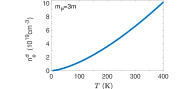
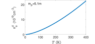
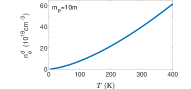
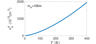
Figure 7: Degenerate density as function of temperature calculated from Eq.(46) for several values of $m_{\text{P}}$.

The degenerate density $n_{e}^{\text{d}}\varpropto m_{\text{P}}^{3/2}$ is sensitive to the choice of $m_{\text{P}}$. In Table.1, $n_{e}^{\text{d}}$ are listed for $T=10$, $20$ and $300$K. We could use Boltzmann distribution (45) only when $n_{e}<(n_{e}^{\text{d}})_{\min}$. When $n_{e}>n_{e}^{\text{d}}$, the gas of EPs or electrons should be described by the Fermi distribution. In the photovoltaic application, $n_{e}\ll\min\{n_{e}^{\text{d}},n_{e}^{\text{c}}\}$. The carriers are non-degenerate EP gas.

Table 1: Degenerate density ($10^{19}$cm^-3) for several typical temperature and polaron effective mass

T \$m_{\text{P}}$	3m	5.1m	10m	100m
10K	0.04	0.09	0.24	7.72
20K	0.11	0.25	0.69	21.83
300K	6.59	14.61	40.11	1268

V.5 Collision mechanisms

The formation energy $E_{\text{EP}}$ of an electron polaron (EP) is larger than the maximal energy $\hbar\omega_{b}$ of an acoustic phonon (9.2meV), and the energy change $v\Delta p\thicksim k_{B}T$ in EP-EP collision ($v$ is the velocity of a polaron, $\Delta p$ is the change in momentum during a collision). Therefore, before an EP annihilating with a hole polaron (HP), an EP is a stable entity, will not break into an electron in three collision mechanisms (EP-EP, EP-defect and EP-Aph).

The charge transport is mainly controlled by three collision mechanisms: (i) EP-EP scattering; (ii) EP-defect scattering; and (iii) absorption or/and emission a LA phonon by a EP. To calculate the mobility of EP with Boltzmann equation, in a ABX₃ sample, let us consider a physical infinitesimal volume Lifshitz and Pitaevskii (1981) $\mathcal{V}$ which contains $\mathcal{N}$ primitive cells.

V.6 EP-EP scattering

The rate $\nu_{\text{PP}}=(\frac{\partial f_{\mathbf{p}}}{\partial t})_{\text{PP}}$ of change in distribution function $f_{\mathbf{p}}$ of EPs caused by EP-EP collisions is Peierls (2001)

$$(\frac{\partial f_{\mathbf{p}}}{\partial t})_{\text{PP}}=\frac{2\pi}{\hbar}\sum_{\mathbf{p}_{2}\mathbf{p}^{\prime}}|\langle\mathbf{p}^{\prime},\mathbf{p}_{2}^{\prime}|H_{\text{PP}}|\mathbf{p},\mathbf{p}_{2}\rangle|^{2}$$

$$\delta(E_{\mathbf{p}}+E_{\mathbf{p}_{2}}-E_{\mathbf{p}^{\prime}}-E_{\mathbf{p}_{2}^{\prime}})$$ (47)

$$\{f_{\mathbf{p}^{\prime}}f_{\mathbf{p}_{2}^{\prime}}(1-f_{\mathbf{p}})(1-f_{\mathbf{p}_{2}})-f_{\mathbf{p}}f_{\mathbf{p}_{2}}(1-f_{\mathbf{p}^{\prime}})(1-f_{\mathbf{p}_{2}^{\prime}})\},$$

where

$$H_{\text{PP}}=\frac{e^{2}}{\epsilon_{0}\mathcal{V}|\mathbf{k}_{2}-\mathbf{k}_{2}^{\prime}|^{2}\varepsilon},\text{ }$$ (48)

is the effective Coulomb interaction between two EPs with momentum $\mathbf{p}$ and $\mathbf{p}_{2}$, $\mathbf{p}_{2}-\mathbf{p}_{2}^{\prime}=\mathbf{p}^{\prime}-\mathbf{p}$ is the momentum exchange during collision, $\mathbf{k}_{2}-\mathbf{k}_{2}^{\prime}=(\mathbf{p}_{2}-\mathbf{p}_{2}^{\prime})/\hbar$. $\varepsilon^{-1}$ is given by Eq.(31).

To estimate the order of magnitude of $\nu_{\text{PP}}$, let us mimic the procedure of Peierls (2001). Consider the second term in Eq.(47). We notice that $f_{\mathbf{p}}=1$, $f_{\mathbf{p}_{2}}$ is given by Eq.(45) by $\varepsilon\rightarrow\varepsilon_{\mathbf{p}_{2}}$. Because $f_{\mathbf{p}^{\prime}}$ and $f_{\mathbf{p}_{2}^{\prime}}\ll 1$, the number in each ( ) can be taken as 1. If one views the energy conservation delta function as a rectangle with width $D$, where $D\thicksim 3$eV is the width of the conduction band Brivio et al. (2014); Menendez-Proupin et al. (2014). Then the height of the delta function is $D^{-1}$. The summations over $\mathbf{p}_{2}$ and $\mathbf{p}^{\prime}$ produces $(k_{B}T\mathcal{V}\frac{dZ}{dE})^{2}$, here $\frac{dZ}{dE}\thicksim a^{-3}D^{-1}$ is the density of states per unit volume per unit energy interval, $a$ is the lattice constant of a primitive cell. The characteristic momentum exchange may be taken as the minimal detectable change in momentum, i.e. the uncertainty of the momentum $\hbar/d$, where $d=2R_{\text{P}}$ is the diameter of a EP. Then the average collision frequency $\nu_{\text{PP}}$ of a EP with other EPs is

$$\nu_{\text{PP}}\thicksim\left[\frac{T}{T_{1}\varepsilon_{s1}+(T-T_{1})\varepsilon_{\infty}}\right]^{2}n_{e}$$ (49)

$$\frac{4\pi^{3/2}\hbar^{3}e^{-\varepsilon_{2}/k_{B}T}}{(2m_{EP}k_{B}T)^{3/2}}\frac{1}{\hbar}\frac{d^{4}}{a^{6}}(\frac{e^{2}}{\epsilon_{0}})^{2}\frac{(kT)^{2}}{D^{3}}\text{.}$$

Because the EP gas is non-degenerate, $n_{e}$ and $m_{\text{P}}^{-3/2}$ appear in $f_{\mathbf{p}_{2}}$, and as a result appear in $\nu_{\text{PP}}$. According to the energy partition theorem, the average energy $\varepsilon_{2}\thicksim 3k_{B}T/2$, then $e^{-\varepsilon_{2}/k_{B}T}\thickapprox e^{-3/2}$ does almost not depend on temperature. If EP-EP collision was the unique collision mechanism, the mobility $\mu=e/\nu_{\text{PP}}m_{EP}$ of EP would be proportional to $n_{e}^{-1}m_{\text{P}}^{1/2}T^{-5/2}$.

V.7 Scattering EP by defects

Denote $C$ as the number of the I^- vacancies per unit volume, the average distance between two vacancies is $\thicksim C^{-1/3}$. The Coulomb scattering amplitude caused by $h_{\text{def}}$ is Landau and Lifshitz (1981); Schiff (1968) $f_{c}\thicksim\Delta z_{\text{I}^{-}}e^{2}/8\pi\epsilon_{0}\varepsilon k_{B}T\thickapprox 1.76$Å, is smaller than $C^{-1/3}$ for a moderate defect concentration. For example, if the concentration of I^- vacancy is 1 in 2 cells ($16.7\%$), the average distance between two I^- vacancies is $\thicksim 7.9$Å. Then one can ignore the interference between two I^- vacancies. In a sample with volume $\mathcal{V}$, there are $C\mathcal{V}$ iodine ions vacancies. The total scattering probability with $C\mathcal{V}$ I^- vacancies is just $C\mathcal{V}$ multiply by the scattering probability with one I^- vacancy.

Comparing to the kinetic energy of an EP, even taken into account the large dielectric constant $\varepsilon\thickapprox 70$ of CH₃NH₃PbI₃, the polaron-defect interaction $h_{\text{P-def}}$ cannot be treated as a perturbation Callaway (2013); Landau and Lifshitz (1981), Born approximation is inapplicable Landau and Lifshitz (1981); Lifshitz and Pitaevskii (1981) to.the scattering of an EP by an I^- vacancy. Fortunately, for Coulomb potential (33), the scattering probability calculated by Fermi’s golden rule is the same as that calculated by the exact method Bohm (1989).

The rate of change in the distribution function of EPs caused by the collisions with I^- vacancies is Lifshitz and Pitaevskii (1981); Callaway (2013)

$$(\frac{\partial f_{\mathbf{p}}}{\partial t})_{\text{P-def}}=\sum_{\mathbf{p}^{\prime}}C\mathcal{V}\frac{2\pi}{\hbar}|\langle\mathbf{p}^{\prime}|h_{\text{P-def}}|\mathbf{p}\rangle|^{2}$$ (50)

$$\delta(E_{\mathbf{p}^{\prime}}-E_{\mathbf{p}})[f_{\mathbf{p}^{\prime}}(1-f_{\mathbf{p}})-f_{\mathbf{p}}(1-f_{\mathbf{p}^{\prime}})],$$

where

$$\langle\mathbf{p}^{\prime}|h_{\text{P-def}}|\mathbf{p}\rangle=\frac{1}{\varepsilon\mathcal{V}\epsilon_{0}}\frac{\Delta z_{\text{I}^{-}}e^{2}}{q^{2}},\text{ }\mathbf{q}=(\mathbf{p}^{\prime}-\mathbf{p})/\hbar.$$ (51)

Let us estimate the average collision frequency $\nu_{\text{P-def}}=(\partial f_{\mathbf{p}}/\partial t)_{\text{P-def}}$ of an EP with defects. Since an I^- vacancy is attached to the perovskite lattice, and the mass of lattice is much larger than $m_{\text{P}}$. The collision of an EP with an I^- vacancy can be viewed as elastic collision, a typical change in wave vector is $q\thicksim\sqrt{2m_{\text{P}}k_{B}T}/\hbar$. $\sum_{\mathbf{p}^{\prime}}$ is over $\mathcal{V}k_{B}TD^{-1}a^{-3}$ electronic states. Viewing the delta function as a rectangle with width $D$, the height of delta function is $\thicksim D^{-1}$. Combine these factors, the rate $\nu_{\text{P-def}}$ of change in the distribution function of EPs caused by the collisions with I^- vacancies is

$$\nu_{\text{P-def}}\thickapprox\left[\frac{T}{T_{1}\varepsilon_{s1}+(T-T_{1})\varepsilon_{\infty}}\right]^{2}C\frac{2\pi}{\hbar}$$ (52)

$$\left(\frac{\Delta z_{\text{I}^{-}}e^{2}}{\epsilon_{0}}\right)^{2}\frac{1}{D^{2}a^{3}}\frac{\hbar^{4}}{(2m_{\text{P}}k_{B}T)^{2}}k_{B}T.$$

The circle line in Fig.8 is $\nu_{\text{P-def}}$ vs. $T$ for a moderate vacancy concentration $C=1/10$cell ($3.33\%$). $\nu_{\text{P-def}}$ is much smaller than $\nu_{\text{P-Aph}}$. However, for $C\thicksim 1/$cell $(33.3\%)$, $\nu_{\text{P-def}}$ is comparable to even surpass $\nu_{\text{P-Aph}}$.

It has been noticed that $\mu$ is not sensitive to the defects in ABX₃ Zhu and Podzorov (2015); Brenner et al. (2015). One of the reasons is that ABX₃ is in a super paraelectric phase, has a larger dielectric function. The polaron-defect interaction is screened by the internal electric field caused by the displacements of the Pb²⁺ and I^- ions: $h_{\text{P-def}}=h_{\text{P-def}}^{\text{bare}}/\varepsilon\ll h_{\text{P-def}}^{\text{bare}}$. According to Eq.(52), $\nu_{\text{P-def}}\thicksim C/\varepsilon^{2}$. If ABX₃ was not in a super paraelectric phase, $\varepsilon$ would be order 1. The polaron-defect scattering would be a far more serious matter.

V.8 Absorption or emission a LA phonon by a EP

The rate $\nu_{\text{P-LA}}=(\partial f_{\mathbf{p}}/\partial t)_{\text{P-LA}}$ of change in the distribution function $f_{\mathbf{p}}$ of EP caused by the P-LA phonon scattering is Lifshitz and Pitaevskii (1981)

$$(\frac{\partial f_{\mathbf{p}}}{\partial t})_{\text{P-LA}}=-\sum_{\mathbf{k}}\frac{\partial N_{0}(\omega)}{\partial\hbar\omega}[f_{0}(\mathbf{p}^{\prime})-f_{0}(\mathbf{p})]$$ (53)

$$\{w(\mathbf{p}^{\prime},\mathbf{k};\mathbf{p})(\varphi_{\mathbf{p}^{\prime}}-\varphi_{\mathbf{p}}+\chi_{\mathbf{k}})\delta(E_{\mathbf{p}}-E_{\mathbf{p}^{\prime}}-\hbar\omega_{\mathbf{k}})$$

$$-w(\mathbf{p}^{\prime};\mathbf{p},\mathbf{k})(\varphi_{\mathbf{p}^{\prime}}-\varphi_{\mathbf{p}}-\chi_{\mathbf{k}})\delta(E_{\mathbf{p}}-E_{\mathbf{p}^{\prime}}+\hbar\omega_{\mathbf{k}})\}$$

where $f_{0}$ and $N_{0}$ are the equilibrium distribution functions at temperature $T$ for EPs and phonons, $\varphi$ and $\chi$ describe the deviations of $f_{\mathbf{p}}$ and $N_{\mathbf{k}}$ from equilibrium

$$f_{\mathbf{p}}-f_{0}(\varepsilon)=-\frac{\partial f_{0}(\varepsilon)}{\partial\varepsilon}\varphi,$$ (54)

and

$$N_{\mathbf{k}}-N_{0}(\mathbf{k})=-\frac{\partial N_{0}(\omega)}{\partial\hbar\omega}\chi.$$ (55)

The probability coefficient $w(\mathbf{p}^{\prime},\mathbf{k};\mathbf{p})$ is defined by

$$\frac{2\pi}{\hbar}|\langle\mathbf{p}^{\prime},\mathbf{k}|h_{\text{P-LA}}(\text{emission})|\mathbf{p}\rangle|^{2}$$ (56)

$$=w(\mathbf{p}^{\prime},\mathbf{k};\mathbf{p})(N_{\mathbf{k}}+1),$$

or

$$\frac{2\pi}{\hbar}|\langle\mathbf{p}^{\prime}|h_{\text{P-LA}}(\text{absorption})|\mathbf{p},\mathbf{k}\rangle|^{2}$$

$$=w(\mathbf{p}^{\prime};\mathbf{p},\mathbf{k})N_{\mathbf{k}}.$$ (57)

Using Eqs.(29,56), one has

$$w\thicksim\frac{\pi\mathcal{N}}{\varepsilon^{2}M\omega k^{2}\mathcal{V}^{2}}(\frac{ze^{2}}{\epsilon_{0}})^{2}.$$ (58)

In calculating transition probability caused by $h_{\text{P-LA}}$, one should be careful that the total probability is NOT the sum of the probabilities caused by the ions in a primitive cell. The interference between ions is vital Zhang and Guo (1994), otherwise will lead to a wrong conclusion: $w=\sum_{i}w_{i}$ which means that the more atoms in a primitive cell, the stronger P-LA interaction.

Let us estimate the change rate $\nu_{\text{P-LA}}=(\frac{\partial f_{\mathbf{p}}}{\partial t})_{\text{P-LA}}$ of distribution function of EP caused by emission or absorption a LA phonon. $\sum_{\mathbf{k}}$ in Eq.(53) represents the summation over all possible phonon states, produces a factor $\mathcal{V}4\pi k_{b}^{3}/3$. The delta function represents the energy conservation during the emission or absorption of a phonon. Since the maximal allowable energy of a phonon is $\hbar\omega_{b}$, the width of the delta function is $\hbar\omega_{b}$. Then the height of delta function is $(\hbar\omega_{b})^{-1}$. For most of the temperature range of photovoltaic application, $\hbar\omega_{b}\ll k_{B}T$, so that Lifshitz and Pitaevskii (1981)

$$\frac{\partial N_{0}(\omega)}{\partial\hbar\omega}\thicksim\frac{k_{B}T}{(\hbar\omega_{b})^{2}}.$$ (59)

Because the characteristic energy of an EP is $\thicksim k_{B}T$ and $\hbar\omega_{b}\ll k_{B}T$, $(\varphi_{\mathbf{p}^{\prime}}-\varphi_{\mathbf{p}}+\chi_{\mathbf{k}})\thicksim k_{B}T$ Lifshitz and Pitaevskii (1981). The delta function in Eq.(53) requires $E_{\mathbf{p}^{\prime}}=E_{\mathbf{p}}\pm\hbar\omega_{\mathbf{k}}$, then

$$f_{0}(\mathbf{p}^{\prime})-f_{0}(\mathbf{p})=\frac{\partial f_{0}(\varepsilon)}{\partial\varepsilon}(E_{\mathbf{p}^{\prime}}-E_{\mathbf{p}})$$

$$\thicksim n_{e}\frac{4\pi^{3/2}\hbar^{3}e^{-\varepsilon/k_{B}T}}{(2m_{\text{P}})^{3/2}(k_{B}T)^{5/2}}\hbar\omega_{b}.$$ (60)

Since we are considering the change of occupation number in state $|\mathbf{p}\rangle$ at the time moment $t$, in Eq.(53), $f_{\mathbf{p}}=1$ at the concerned moment $t$ Peierls (2001). Combine above considerations, one has

$$\nu_{\text{P-LA}}\thicksim\left[\frac{T}{T_{1}\varepsilon_{s1}+(T-T_{1})\varepsilon_{\infty}}\right]^{2}\frac{\pi}{M\omega_{b}k_{b}^{2}a^{3}}$$

$$\frac{4\pi}{3}k_{b}^{3}(\frac{ze^{2}}{\epsilon_{0}})^{2}(\frac{k_{B}T}{\hbar\omega_{b}})^{2}n_{e}\frac{4\pi^{3/2}\hbar^{3}e^{-\varepsilon/k_{B}T}}{(2m_{EP})^{3/2}(k_{B}T)^{5/2}}.$$ (61)

In Fig.8, Eqs.(49,52,61) are plotted against $T$ for $n_{e}=10^{18}$cm^-1, $m_{\text{P}}=10m$, $\varepsilon(\omega_{b})=36.5$ [which are different to those for Fig.3 in the text]. One can see that relation $\nu_{\text{P-LA}}\gg\nu_{\text{P-def}}\gg\nu_{\text{PP}}$ is not sensitive to the choice of $m_{\text{P}}$ and $\varepsilon$. One can also see $\nu_{\text{P-Aph}}\gg\nu_{\text{P-def}}$ intuitively: (1) the available states for the EP-defect scattering produce a factor $1/D^{2}$, while for the P-Aph process produce a factor $(\hbar\omega_{D})^{-2}$, $1/D^{2}\ll(\hbar\omega_{D})^{-2}$; (2) the probability of P-Aph interaction is proportional to $N_{\omega}$ which is a large number because the acoustic modes are fully excited.

We calculate $\mu(T)$ with the experimental $\varepsilon(\omega,T)$ for $\omega/2\pi=1$KHz obtained in Onoda-Yamamuro et al. (1992) instead of $\varepsilon_{\infty}+C(\omega)/T$, i.e. in Eqs.(49,52,61) replace $\left[\frac{T}{300\varepsilon_{s1}+(T-300)\varepsilon_{\infty}}\right]^{2}$ by $[\varepsilon(\omega_{b},T)]^{-2}$, where $\varepsilon(\omega_{b},T)=[\varepsilon(\omega/2\pi=1$KHz$,T)+\varepsilon_{\infty}]/2$. The general trend of $\mu(T)$ observed in [Hutter et al., 2017] is reproduced: in tetragonal phase $\mu(T)\varpropto T^{-3/2}$, while in the orthorhombic phase $\mu(T)$ decreases with decreasing temperature. Due to the samples in [Hutter et al., 2017]  and in [Onoda-Yamamuro et al., 1992] are different, the transition temperature in [Hutter et al., 2017] is 150K, while in [Onoda-Yamamuro et al., 1992] is 160K. But the general trend of $\mu(T)$ in orthorhombic phase Hutter et al. (2017) is reproduced by the current model with experimental dielectric function of [Onoda-Yamamuro et al., 1992]. If one assumes that (i) the sample in [Hutter et al., 2017] is more uniform and is annealed slowly, below 150K, only orthorhombic phase exists; (ii) both tetragonal phase and orthorhombic phase coexist Kong et al. (2015); Hutter et al. (2017) in the samples of earlier work Oga et al. (2014); Savenije et al. (2014); Milot et al. (2015) at $T<150$K; then the two observations can be conciliated.

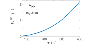
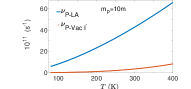
Figure 8: $m_{\text{P}}=10m$, $n_{e}=10^{18}$cm^-3, $c_{s}=2147$ m/s, using last step of Eq.(31) and $\varepsilon(\omega_{0})=36.5$. (a) PP collision frequency $\nu_{\text{PP}}$ as a function of temperature determined by Eq.(49). (b) P-LA collision frequency $\nu_{\text{P-LA}}$ and P-Vac collision frequency $\nu_{\text{P-Vac I${}^{-}$}}$ as functions of temperature determined by Eq.(61) and Eq.(52). $\nu_{\text{P-LA}}$ is the main scattering mechanism.

The total collision frequency $\nu_{t}$ of an EP is the summation of all three processes:

$$\nu_{t}=\nu_{\text{P-LA}}+\nu_{\text{P-def}}+\nu_{\text{PP}}.$$ (62)

The mobility is

$$\mu=\frac{e}{\nu_{t}m_{\text{P}}}.$$ (63)

From Eqs.(49,52,61), we have seen that collision frequencies and $\mu$ depend on $\varepsilon(\omega,T)$. There are some discrepancies among the experimental dielectric functions obtained by different authors. For example, $\varepsilon_{0}\thickapprox 33$ according to Poglitsch and Weber (1987); Frost et al. (2014a) instead of $\varepsilon_{0}\thickapprox 70$ Lin et al. (2015); Onoda-Yamamuro et al. (1992), that may due to the differences in the compositions, structures, status of samples and the methods of measurement. The dielectric functions calculated by different methods are not far from each other $\varepsilon_{0}\thickapprox 24.5$, about two times smaller than the well cited experimental value $\varepsilon_{0}\thickapprox 70$ Lin et al. (2015); Onoda-Yamamuro et al. (1992); Sewvandi et al. (2016a, b). In Fig.9, we made a fitting with $\varepsilon_{0}\thickapprox 70$, which anticipates a higher concentration of carriers. However, Eq.(63) is only for the mobility $\mu_{e}$ of EPs. The hole mobility $\mu_{h}$ has the same order of magnitude as $\mu_{e}$. The measured mobility is $\phi(\mu_{e}+\mu_{h})$, where $\phi$ is the quantum efficiency of photon. If we plot $(\mu_{e}+\mu_{h})$ rather than just $\mu_{e}$, $\varepsilon_{0}\thickapprox 70$ would suggest a similar carrier concentration as that obtained in Fig.5 in text.

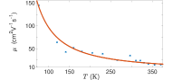
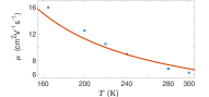
Figure 9: Mobility calculated with Eqs.(49,52,61,62,63)(solid line) and exact Eq.(31), dielectric function $\varepsilon_{0}=70$, $\varepsilon_{\infty}=6.5$ taken from measurement Lin et al. (2015). (a) Experimental data (crosses) from Milot et al. (2015), $n_{e}=1.2\times 10^{18}$cm^-3. (b) Experimental data (squares) from Savenije et al. (2014), $n_{e}=4.1\times 10^{18}$cm^-3.

V.9 Decreases of vibrational entropy in a polaron

The frequency $\omega_{1}$ of Pb-I stretch mode is increased in a polaron which leads to the decrease of vibrational entropy. To estimate the decrease of vibrational entropy, we apply the Morse potential

$$V(r)=D[1-e^{-\sigma(r-r_{e})}]^{2},$$ (64)

to describe the potential energy of the Pb²⁺ and I^- interaction, where $\sigma$ is a positive number, $D$ is the dissociation energy of Pb-I bond, $r$ is the distance between Pb²⁺ and I^- ion, $r_{e}=3.15$Å is the equilibrium distance between Pb²⁺ and I^- in a normal lattice without the static deformation inside an EP.

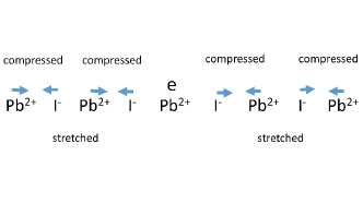
Figure 10: Schematic sketch of the deformation in an EP: Pb-I bonds are compressed and stretched alternatively by the extra electron in the center of polaron.

In an EP, Pb-I bonds are alternatively compressed and stretched, cf. Fig.10. These static deformations make the Pb-I distances are smaller and larger than $r_{e}$. If the distance between Pb and I is fixed at $r$, the spring constant $k(r)$ is

$$k(r)=\frac{d^{2}V(r)}{dr^{2}}=2D\sigma^{2}[2e^{-2\sigma(r-r_{e})}-e^{-\sigma(r-r_{e})}].$$ (65)

The positive number $\sigma$ in Eq.(64) is determined by

$$\sigma=\sqrt{\frac{k(r_{e})}{2D}}.$$ (66)

Then, Eq.(65) becomes

$$k(r)=k(r_{e})[2e^{-2\sigma(r-r_{e})}-e^{-\sigma(r-r_{e})}].$$ (67)

One can easily check

$$\frac{dk(r)}{dr}=2D\sigma^{3}[e^{-\sigma(r-r_{e})}-4e^{-2\sigma(r-r_{e})}],$$ (68)

and

$$\frac{d^{2}k(r)}{dr^{2}}=2D\sigma^{4}[8e^{-2\sigma(r-r_{e})}-e^{-\sigma(r-r_{e})}].$$ (69)

From Eq.(68), one can see $\frac{dk(r)}{dr}|_{r=r_{e}}=0$. From Eq.(69), one can see $\frac{d^{2}k(r)}{dr^{2}}>0$ for

$$r<r_{e}+\sqrt{\frac{2D}{k(r_{e})}}\ln 8.$$ (70)

Above two facts mean that $r=r_{e}$ is a minimum of $k(r)$. The spring constant of the stretch mode of Pb-I bond can be estimated from $k(r_{e})=m_{r}\omega_{\text{LO}}^{2}$, where $m_{r}$ is the reduced mass of Pb ion and I ion. If one takes $\omega_{\text{LO}}=100$cm^-1, $k(r_{e})=46.4$N/m. The bond energy of Pb-I is $D=142$KJ/mol [http://www.chem.tamu.edu/rgroup

/connell/linkfiles/bonds.pdf], then $\sqrt{\frac{2D}{k(r_{e})}}\ln 8=2.1$Å. From Eq.(66), $\sigma=9.92\times 10^{9}$m^-1.

Consider an ion with charge $q_{i}$, denote the distance between the extra electron and the ion as $x$, then the static displacement caused by the extra electron is

$$d(x,q_{i})=\frac{1}{4\pi\epsilon_{0}}\frac{eq_{i}}{k_{e}\varepsilon_{0}x^{2}},$$ (71)

where $k_{e}=k(r_{e})$ is spring constant of Pb-I bond in a normal crystal, $\varepsilon_{0}$ is the static dielectric function. To get an upper limit of $d(x,q_{i})$, let us take $\varepsilon_{0}=24.5$, $x=3.15$Å, $q_{i}=e$, then the largest possible static displacement of I^- ion $d(x,q_{i})=0.02$Å$\ll\sqrt{\frac{2D}{k(r_{e})}}\ln 8$. In an EP, even for the stretched Pb-I bond, condition (70) is still satisfied. Since $r=r_{e}$ is a minimum of $k(r)$ under condition (70), both the compressed Pb-I bond and the stretched Pb-I bond have larger spring constants $k(r)$, i.e. larger vibrational frequency $\omega_{1}=\sqrt{\frac{k(r)}{m_{r}}}>\omega_{\text{LO}}$, which leads to a smaller vibrational entropy in a polaron relative to that of an electron in the undeformed lattice.

References

- Grancini et al. (2015) G. Grancini, A. R. S. Kandada, J. M. Frost, A. J. Barker, M. D. Bastiani, M. Gandini, S. Marras, G. Lanzani, A. Walsh, and A. Petrozza, Nature Photonics 9, 695–701 (2015).
- Dong et al. (2015) Q. Dong, Y. Fang, Y. Shao, P. Mulligan, J. Qiu, L. Cao, and J. Huang, Science 347, 967 (2015).
- Saidaminov et al. (2015) M. I. Saidaminov, A. L. Abdelhady, B. Murali, E. Alarousu, V. M. Burlakov, W. Peng, I. Dursun, L. Wang, Y. He, G. Maculan, A. Goriely, T. Wu, O. F. Mohammed, and O. M. Bakr, Nature Communications 6, 7586 (2015).
- Bi et al. (2014) C. Bi, Y. Shao, Y. Yuan, Z. Xiao, C. Wang, Y. Gao, and J. Huang, J. Mater. Chem. A 2, 18508 (2014).
- Oga et al. (2014) H. Oga, A. Saeki, Y. Ogomi, S. Hayase, and S. Seki, Journal of the American Chemical Society 136, 13818 (2014).
- Milot et al. (2015) R. L. Milot, G. E. Eperon, H. J. Snaith, M. B. Johnston, and L. M. Herz, Advanced Functional Materials 25, 6218 (2015).
- Savenije et al. (2014) T. J. Savenije, C. S. Ponseca, L. Kunneman, M. Abdellah, K. Zheng, Y. Tian, Q. Zhu, S. E. Canton, I. G. Scheblykin, T. Pullerits, A. Yartsev, and V. Sundström, The Journal of Physical Chemistry Letters 5, 2189 (2014).
- Karakus et al. (2015) M. Karakus, S. A. Jensen, F. D’Angelo, D. Turchinovich, M. Bonn, and E. Cánovas, The Journal of Physical Chemistry Letters 6, 4991 (2015).
- Hutter et al. (2017) E. M. Hutter, M. C. Gelvez-Rueda, A. Osherov, V. Bulovic, F. C. Grozema, S. D. Stranks, and T. J. Savenije, Nat Mater 16, 115 (2017).
- Zhu and Podzorov (2015) X.-Y. Zhu and V. Podzorov, The Journal of Physical Chemistry Letters 6, 4758 (2015).
- Brenner et al. (2015) T. M. Brenner, D. A. Egger, A. M. Rappe, L. Kronik, G. Hodes, and D. Cahen, The Journal of Physical Chemistry Letters 6, 4754 (2015).
- Wright et al. (2016) A. D. Wright, C. Verdi, R. L. Milot, G. E. Eperon, M. A. Pe´rez-Osorio, H. J. Snaith, F. Giustino, M. B. Johnston1, and L. M. Herz, Nature Communications 7, 11755 (2016).
- Sendner et al. (2016) M. Sendner, P. K. Nayak, D. A. Egger, S. Beck, C. Muller, B. Epding, W. Kowalsky, L. Kronik, H. J. Snaith, A. Pucci, and R. Lovrincic, Mater. Horiz. 3, 613 (2016).
- Callaway (2013) J. Callaway, Quantum Theory of the Solid State, 2nd ed. (Academic Press, 2013).
- Emin (2013) D. Emin, Polarons (Cambridge University Press, 2013).
- EnvironmentalChemistry.com (2016) EnvironmentalChemistry.com, http://environmentalchemistry.com/yogi/periodic/ionicradius.html (2016).
- Wikipedia (2016) Wikipedia, https://en.wikipedia.org/wiki/Ionic_radius (2016).
- Lin et al. (2015) Q. Lin, A. Armin, R. C. R. Nagiri, P. L. Burn, and P. Meredith, Nat Photon 9, 106 (2015).
- Onoda-Yamamuro et al. (1992) N. Onoda-Yamamuro, T. Matsuo, and H. Suga, Journal of Physics and Chemistry of Solids 53, 935 (1992).
- Frost et al. (2014a) J. M. Frost, K. T. Butler, and A. Walsh, APL Materials 2, 081506 (2014a).
- Brivio et al. (2014) F. Brivio, K. T. Butler, A. Walsh, and M. van Schilfgaarde, Phys. Rev. B 89, 155204 (2014).
- Menendez-Proupin et al. (2014) E. Menendez-Proupin, P. Palacios, P. Wahnon, and J. C. Conesa, Physical Review B 90, 045207 (2014).
- Bokdam et al. (2016) M. Bokdam, T. Sander, A. Stroppa, S. Picozzi, D. D. Sarma, C. Franchini, and G. Kresse, Scientific Reports 6, 28618 (2016).
- Frost (2017) J. M. Frost, arXiv.org (2017), arXiv:1704.05404v3 [cond-mat.trl-sci] .
- Landau and Lifshitz (1980) L. D. Landau and E. M. Lifshitz, Statistical Physics, Part 1, 3rd ed. (Butterworth-Heinemann, 1980).
- Chen et al. (2016) Y. Chen, H. T. Yi, X. Wu, R. Haroldson, Y. N. Gartstein, Y. I. Rodionov, K. S. Tikhonov, A. Zakhidov, X. Y. Zhu, and V. Podzorov, Nature Communications 7, 12253 (2016).
- Hill (1987) T. L. Hill, An Introduction to Statistical Thermodynamics (Dover Publications, 1987).
- Zeghbroeck (2011) B. V. Zeghbroeck, “Principles of semiconductor devices,” http://ecee.colorado.edu/~bart/book/book/chapter2/ch2_7.htm (2011).
- Feynman et al. (1977) R. P. Feynman, R. B. Leighton, and M. Sands, The Feynman Lectures on Physics, Vol. 2 (Addison-Wesley, 1977).
- Zhang et al. (2017) M.-L. Zhang, X. Zhang, L.-Y. Huang, H.-Q. Lin, and G. Lu, Supplemental Material http://link.aps.org/supplemental/ (2017).
- Schwinger et al. (1998) J. Schwinger, L. L. Deraad Jr., K. A. Milton, W.-Y. Tsai, and J. Norton, Classical Electrodynamics (Westview Press, 1998).
- Poglitsch and Weber (1987) A. Poglitsch and D. Weber, The Journal of Chemical Physics 87, 6373 (1987).
- Kittel (1976) C. Kittel, Solid State Physics, 5th ed. (John Wiley, 1976).
- Frost et al. (2014b) J. M. Frost, K. T. Butler, F. Brivio, C. H. Hendon, M. van Schilfgaarde, and A. Walsh, Nano Letters 14, 2584 (2014b).
- Leguy et al. (2015a) A. M. A. Leguy, J. M. Frost, A. P. McMahon, V. G. Sakai, W. Kockelmann, C. Law, X. Li, F. Foglia, A. Walsh, B. C. O’Regan, J. Nelson, J. T. Cabral, and P. R. F. Barnes, Nature Communications 6, 7124 (2015a).
- Wasylishen et al. (1985) R. E. Wasylishen, O. Knop, and J. B. Macdonald, Solid State Communications 56, 581 (1985).
- Kittel (1987) C. Kittel, Quantum Theory of Solids, 2nd ed. (Wiley, 1987).
- Feynman (1955) R. P. Feynman, Phys. Rev. 97, 660 (1955).
- Menéndez-Proupin et al. (2015) E. Menéndez-Proupin, C. L. Beltrán Ríos, and P. Wahnón, Physica Status Solidi (RRL) – Rapid Research Letters 9, 559 (2015).
- Lifshitz and Pitaevskii (1981) E. M. Lifshitz and L. P. Pitaevskii, Physical Kinetics, 1st ed. (Butterworth-Heinemann, 1981).
- He and Galli (2014) Y. He and G. Galli, Chemistry of Materials 26, 5394 (2014).
- Qian et al. (2016) X. Qian, X. Gu, and R. Yang, Applied Physics Letters 108, 063902 (2016).
- Peierls (2001) R. E. Peierls, Quantum Theory of Solids (Oxford University Press, 2001).
- Umari et al. (2014) P. Umari, E. Mosconi, and F. D. Angelis, Scientific Reports 4, 4467 (2014).
- Yin et al. (2015) W.-J. Yin, J.-H. Yang, J. Kang, Y. Yan, and S.-H. Wei, J. Mater. Chem. A 3, 8926 (2015).
- Yin et al. (2014) W.-J. Yin, T. Shi, and Y. Yan, Applied Physics Letters 104, 063903 (2014).
- Miller (2014) J. L. Miller, Physics Today 67, 11 (2014).
- Kong et al. (2015) W. Kong, Z. Ye, Z. Qi, B. Zhang, M. Wang, A. Rahimi-Iman, and H. Wu, Phys. Chem. Chem. Phys. 17, 16405 (2015).
- Brivio et al. (2013) F. Brivio, A. B. Walker, and A. Walsh, APL Mater. 1, 042111 (2013).
- Mosconi et al. (2014) E. Mosconi, C. Quarti, T. Ivanovska, G. Ruani, and F. De Angelis, Phys. Chem. Chem. Phys. 16, 16137 (2014).
- Quarti et al. (2015) C. Quarti, E. Mosconi, and F. De Angelis, Phys. Chem. Chem. Phys. 17, 9394 (2015).
- Tessman et al. (1953) J. R. Tessman, A. H. Kahn, and W. Shockley, Phys. Rev. 92, 890 (1953).
- Leguy et al. (2015b) A. M. A. Leguy, J. M. Frost, A. P. McMahon, V. G. Sakai, W. Kockelmann, C. Law, X. Li, F. Foglia, A. Walsh, B. C. O’Regan, J. N. abd Joa˜o T. Cabral, and P. R. F. Barnes, The Journal of Physical Chemistry Letters 6, 7124 (2015b).
- HomePage (2016) C. HomePage, CAcT HomePage http://www.science.uwaterloo.ca/~cchieh/cact/c123/tetrahed.html (2016).
- Juarez-Perez et al. (2014) E. J. Juarez-Perez, R. S. Sanchez, L. Badia, G. Garcia-Belmonte, Y. S. Kang, I. Mora-Sero, and J. Bisquert, The Journal of Physical Chemistry Letters 5, 2390 (2014).
- Pines and Nozieres (1966) D. Pines and P. Nozieres, The Theory of Quantum Liquids, Vol. I Normal Fermi Liquids (W. A. Benjamin, 1966).
- Kutes et al. (2014) Y. Kutes, L. Ye, Y. Zhou, S. Pang, B. D. Huey, and N. P. Padture, The Journal of Physical Chemistry Letters 5, 3335 (2014).
- Fan et al. (2015) Z. Fan, J. Xiao, K. Sun, L. Chen, Y. Hu, J. Ouyang, K. P. Ong, K. Zeng, and J. Wang, The Journal of Physical Chemistry Letters 6, 1155 (2015).
- Kim et al. (2015) H.-S. Kim, S. K. Kim, B. J. Kim, K.-S. Shin, M. K. Gupta, H. S. Jung, S.-W. Kim, and N.-G. Park, The Journal of Physical Chemistry Letters 6, 1729 (2015).
- Ziman (1972) J. M. Ziman, Principles of the Theory of Solids, 2nd ed. (Cambridge University Press, 1972).
- Landau and Lifshitz (1981) L. D. Landau and E. M. Lifshitz, Quantum Mechanics, 3rd ed. (Butterworth-Heinemann, 1981).
- Schiff (1968) L. I. Schiff, Quantum Mechanics, 3rd ed. (Mcgraw-Hill College, 1968).
- Bohm (1989) D. Bohm, Quantum Theory, Revised (Dover Publications, 1989).
- Zhang and Guo (1994) M.-L. Zhang and H.-Y. Guo, Physics Letters A 191, 189 (1994).
- Sewvandi et al. (2016a) G. A. Sewvandi, K. Kodera, H. Ma, S. Nakanishi, and Q. Feng, Scientific Reports 6, 30680 (2016a).
- Sewvandi et al. (2016b) G. A. Sewvandi, D. Hu, C. Chen, H. Ma, T. Kusunose, Y. Tanaka, S. Nakanishi, and Q. Feng, Phys. Rev. Applied 6, 024007 (2016b).