The effect of non-sphericity on mass and anisotropy measurements in dSph galaxies with Schwarzschild method

Abstract

In our previous work we confirmed the reliability of the spherically symmetric Schwarzschild orbit-superposition method to recover the mass and velocity anisotropy profiles of spherical dwarf galaxies. Here we investigate the effect of its application to intrinsically non-spherical objects. For this purpose we use a model of a dwarf spheroidal galaxy formed in a numerical simulation of a major merger of two disky dwarfs. The shape of the stellar component of the merger remnant is axisymmetric and prolate which allows us to identify and measure the bias caused by observing the spheroidal galaxy along different directions, especially the longest and shortest principal axis. The modelling is based on mock data generated from the remnant that are observationally available for dwarfs: projected positions and line-of-sight velocities of the stars. In order to obtain a reliable tool while keeping the number of parameters low we parametrize the total mass distribution as a radius-dependent mass-to-light ratio with just two free parameters we aim to constrain. Our study shows that if the total density profile is known, the true, radially increasing anisotropy profile can be well recovered for the observations along the longest axis whereas the data along the shortest axis lead to the inference an incorrect, isotropic model. On the other hand, if the density profile is derived from the method as well, the anisotropy is always underestimated but the total mass profile is well recovered for the data along the shortest axis whereas for the longest axis the mass content is overestimated.

1 Introduction

Galaxies in the observed Universe are divided into a few distinct morphological types based primarily on their shapes, sizes, the nature of their stellar populations and gas content. Giant ellipticals are dominated by non-spherical stellar components. While elliptical galaxies are expected to be embedded in a dark matter halo, the baryons (primarily an old stellar population) tend to dominate the dynamics over most of the region where the stars are found. Spiral galaxies are characterized by a thin stellar disk containing gas which is actively forming stars and older central components which often include a stellar bulge, a stellar bar and a supermassive black hole. Although the dynamics of gas and stars in the outer regions are strongly affected by dark matter, inner regions are still baryon dominated. Baryons also dominate much of the dynamics for smaller dwarf elliptical and dwarf irregular galaxies.

For all these types of galaxies a significant fraction of the total mass in the central parts is contained in the visible components: stars and gas. The situation is different for dwarf spheroidal (dSph) and ultra-faint (UFD) galaxies. Their high line-of-sight velocity dispersions cannot be explained within Newtonian dynamics without the addition of heavy (when compared to the mass in stars) dark matter haloes. Estimated ratios between the masses of dark and baryonic matter in dwarf galaxies reach hundreds (Mateo 1998, Gilmore et al. 2007). They are thought to have formed in the least massive haloes and during their evolution accreted or been able to retain much less baryonic matter (Governato et al. 2010, Sawala et al. 2016).

While the mass enclosed within some characteristic radius can be determined with simple estimators, independent of the orbit anisotropy (Walker et al. 2009, Wolf et al. 2010), detailed studies of mass distribution require more sophisticated methods. The most widely used method is based on solving the spherical Jeans equation (Binney & Tremaine, 2008) but this method suffers from the well known mass-velocity anisotropy degeneracy (Binney & Mamon, 1982) since the velocity anisotropy cannot be determined directly. Significant improvements to the Jeans equation method have been made by including kurtosis in a fitting procedure which partially lifts the mass-anisotropy degeneracy (Łokas, 2002; Łokas et al., 2005). However, the assumptions regarding the spherical symmetry and a particular form of the velocity anisotropy profile are usually necessary.

A more general method that does not require such assumptions is the orbit superposition Schwarzschild modelling (Schwarzschild, 1979). It has been successfully used in the last few decades in modelling ellipticals and bulges with spherically symmetric, axisymmetric and triaxial codes (van der Marel et al. 1998, Cretton et al. 1999, Gebhardt et al. 2003, Valluri et al. 2004, Thomas et al. 2004, Cretton & Emsellem 2004, Cappellari et al. 2006, van den Bosch & de Zeeuw 2010). Recently, it has also been applied to dwarf spheroidals, generally assuming sphericity of both stars and dark matter halo, and focusing on studying the inner slope of the density profile of the halo (Breddels et al. 2013, Breddels & Helmi 2013, Jardel & Gebhardt 2012, Jardel et al. 2013).

Unfortunately, observed shapes of dwarf galaxies in the Local Group show non-negligible ellipticities (McConnachie, 2012). It can be explained within a scenario in which dwarf galaxies were accreted by their hosts as disky and require long evolution on a tight orbit to become spherical (Łokas et al. 2012, Kazantzidis et al. 2013). Non-spherical dwarfs are also the most natural outcome of mergers between disky dwarfs, as we discuss below. Note that both simulations of mergers and tidal evolution of rotationally supported dwarfs favor prolate and triaxial shapes over oblate ones (Kazantzidis et al., 2011a, b). Nevertheless, a possible impact of the ellipticity should not be a reason to relinquish spherically symmetric modelling methods. Their ostensible simplicity proves to be their strength when, as for dwarfs, available data are limited and a low number of free parameters of a model is desired.

Such simplification, however, necessarily leads to systematic errors in the results. Therefore, when deciding to proceed with a spherically symmetric method, it is very important to be aware of the existing biases and their magnitude. They can be measured by applying the method to mock data obtained by observing similar objects formed in numerical simulations along different lines of sight. Such studies have been done for the simple mass estimators mentioned before. Kowalczyk et al. (2013) measured the bias caused by the triaxiality of the stellar component and compared the masses estimated for simulated dwarfs as a function of the axis ratio. They showed that the mass is underestimated when the line of sight towards the galaxy is aligned with the shortest axis of the stellar component, fairly well recovered for the intermediate axis and overestimated by up to a factor of two for the longest one. Campbell et al. (2017) applied a slightly different approach to more advanced simulations, averaging over many lines of sight in order to derive the mean and proving that on average the estimators are unbiased.

In spite of applying the spherically symmetric Schwarzschild method to dwarf spheroidals of the Local Group, no similar work has been done in order to measure biases caused by non-sphericity in this approach. Until now only Jardel & Gebhardt (2012) attempted to take into account the ellipticity when modelling the Fornax dSph. However, in this case they assumed a particular orientation of the galaxy, avoiding an additional parameter.

As we have demonstrated in Kowalczyk et al. (2017), the Schwarzschild method recovers the mass and anisotropy profiles reasonably well for spherical objects. In order to extend the applicability of the method, we decided to test our procedure on simulated data for a dwarf spheroidal galaxy, measuring the influence of the line of sight: on the recovered anisotropy under the assumption of the known density profile and on the recovery of both mass and anisotropy profiles. It will enable us to better understand and assess the validity of future results on modelling observational data.

The paper is organized as follows. In Sec. 2 we introduce the numerical simulation and describe the properties of the galaxy used in this study to generate the mock observations in Sec. 3. In Sec. 4 we present our modelling method and apply it to the mock data, and in Sec. 5 we limit the data samples to the size that is currently available observationally. We summarize and discuss the results in Sec. 6.

2 Major merger simulation

Kazantzidis et al. (2011b), Łokas et al. (2014) and Ebrová & Łokas (2015) have shown that major mergers of two disky dwarfs can produce realistic dwarf spheroidal galaxies. Therefore, for the purpose of this study we simulated a collision of two identical dwarfs, each initially composed of an exponential stellar disc with the total mass $M_{s}=2\times 10^{7}$ M_☉, the scale-length $R_{s}=0.41$ kpc and thickness $z_{s}/R_{s}=0.2$ embedded within a Navarro-Frenk-White-like (NFW, Navarro et al. 1997) spherical dark matter halo of virial mass $M_{DM}=10^{9}$ M_☉ and concentration $c=20$. The $N$-body realizations were generated using procedures of Widrow & Dubinski (2005) and Widrow et al. (2008). Each component of each dwarf was built of $2\times 10^{5}$ particles, giving $8\times 10^{5}$ particles in total. We ran the simulation using $N$-body code GADGET-2 (Springel, 2005) for the total time of 10 Gyr, saving 201 outputs. The adopted softening scales were $\epsilon_{s}=0.02$ kpc and $\epsilon_{DM}=0.06$ kpc for stellar and dark matter particles, respectively.

At the beginning of the simulation the dwarfs were placed at the relative distance of $d=50$ kpc and had the relative radial velocity $v_{orb}=16$ km s^-1. By assigning no tangential component to the relative velocity we skipped the inspiralling phase of merging. The angular momentum vectors of the discs were inclined by 45 deg with respect to the plane of collision and by 90 deg with respect to each other. The galaxies merged during their 3rd approach, after $t_{merge}=3.7$ Gyr from the beginning of the simulation.

For further analysis we used the last snapshot from the simulation taken after 10 Gyr from the beginning when the galaxy is well relaxed. In Fig. 1 we present the colour maps of the surface mass density, line-of-sight velocity and line-of-sight velocity dispersion (from top to bottom) for the observations along the three principal axes of the stellar component: the shortest $z$, intermediate $y$ and longest $x$ (in columns from the left to the right) for stars and dark matter particles (left and right-hand side panels, respectively). As the number of dark matter particles in the central part of the galaxy ($4\times 4$ kpc) is smaller, we reduced the resolution of these maps by a factor of 4.

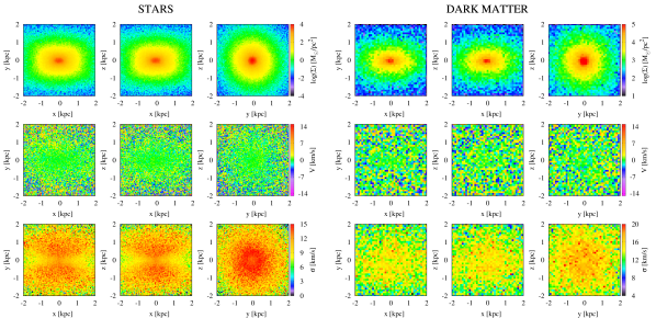
Figure 1: Colour maps of the observed parameters of stars (3 $\times$ 3 panels on the left-hand side) and dark matter (right-hand side) in the final output of the simulation of the major merger. The resolution for dark matter is lower as the number of particles in the central part of the galaxy is smaller. In rows: projected mass density (in logarithm), line-of-sight velocity and line-of-sight velocity dispersion, respectively. In columns: observations along the shortest axis $z$, intermediate $y$ and longest $x$.

Both the stellar component and the dark matter halo are elongated in a similar way with only a few degrees offset between the directions of principal axes. The axis ratios measured within the radius of 0.5 kpc are: shortest to longest $c/a=$0.84 (0.83 for dark matter) and shortest to intermediate $c/b=$0.98 (0.99 or 1.01 for dark matter, as the axes are switched with respect to the stellar component).

In contrast to Łokas et al. (2014) and Ebrová & Łokas (2015) who aimed to obtain prolate rotation (rotation around the major axis of the remnant) as a result of the merger, our galaxy retained no net rotation as the components of the angular momentum vectors of the dwarfs along the axis of collision had opposite directions. Despite the small ellipticity of the remnant, the line-of-sight velocity dispersion map reveals interesting, butterfly-like shape for the lines of sight towards the galaxy perpendicular to the major axis, probably due to the long-axis tube orbits characteristic of prolate spheroids. It may strongly affect the results of any spherically symmetric modelling with respect to axisymmetric models. However, any attempt to account for this is beyond the scope of the present paper.

3 Mock data

By observing the galaxy along each of the principal axes of the stellar component we obtained three mock datasets. For each direction we saved the projected distances from the centre of the galaxy and the line-of-sight velocities of the stars. We will refer to the datasets for observations along the longest/intermediate/shortest axis as ‘$x/y/z$ axis’.

We present the surface mass density profiles of stars with points in the top panel of Fig. 2, where colours: red, orange and blue, denote the line of sight: $x$, $y$ and $z$, respectively. We modelled them with the Sérsic distribution (Sérsic, 1968):

$$n_{\star}(R)=n_{0}\,{\rm exp}[-(R/R_{s})^{1/m}],$$ (1)

where $n_{0}$ is the normalization, $R_{s}$ is the characteristic radius and $m$ is the Sérsic index. The best-fitting profiles for each line of sight are shown in Fig. 2 with lines of corresponding colour and their parameters are listed in Table 1. Thin vertical lines restrict the radial range of fitting: the inner boundary corresponds to minimal credible spatial separation, i.e. 3 softening lengths for the stellar particles in the simulation whereas the outer one mimics the limiting surface brightness in observations and cuts off visible tails.

Table 1: Parameters of the best-fitting Sérsic profiles.

parameter	$x$ axis	$y$ axis	$z$ axis
large samples (all stars)
normalization, $n_{0}$ [$10^{7}\,$M☉ kpc-2]	13.60	7.40	7.08
characteristic radius, $R_{s}$ [kpc]	0.080	0.132	0.145
Sérsic index, $m$	1.825	1.661	1.620
total mass, $M_{s}$ [$10^{7}\,$M☉]	3.973	3.800	3.803
small samples (100 000 stars)
normalization, $n_{0}$ [$10^{7}\,$M☉ kpc-2]	13.49	–	6.95
characteristic radius, $R_{s}$ [kpc]	0.082	–	0.148
Sérsic index, $m$	1.818	–	1.607
total mass, $M_{s}$ [$10^{7}\,$M☉]	3.973	–	3.795

Under the assumption of spherical symmetry, any Sérsic distribution can be deprojected (, Lima, Gerbal & Márquez1999). The 3-dimensional density profile is then given as:

$$\nu_{\star}(r)=\nu_{0}\Big{(}\frac{r}{R_{s}}\Big{)}^{-p}{\rm exp}\bigg{[}-\Big{(}\frac{r}{R_{s}}\Big{)}^{1/m}\bigg{]},$$ (2)

where

$$\nu_{0}=\frac{n_{0}\Gamma(2m)}{2R_{s}\Gamma\Big{(}(3-p)m\Big{)}},$$ (3)

$$p=1-0.6097/m+0.05463/m^{2},$$ (4)

and $\Gamma(x)$ is the standard gamma function. We present the density profiles resulting from our surface density fits in the middle panel of Fig. 2. In addition we show the real 3-dimensional stellar mass density measured from the simulation with green points.

By integrating eq. (2) over a spherical volume we obtain the profile of the cumulative mass of stars:

$$M_{\star}(r)=M_{s}\,\gamma\bigg{(}(3-p)m,\,\Big{(}\frac{r}{R_{s}}\Big{)}^{1/m}\bigg{)},$$ (5)

where

$$M_{s}=\int\limits_{0}\limits^{\infty}4\pi r^{2}\nu_{\star}(r)\,\mathrm{d}r$$ (6)

is the total mass of stars and $\gamma(\alpha,\,x)$ is the normalized incomplete gamma function defined as:

$$\gamma(\alpha,\,x)=\frac{1}{\Gamma(\alpha)}\int\limits_{0}\limits^{x}e^{-t}t^{\alpha-1}\,\mathrm{d}t.$$ (7)

The profiles of the cumulative mass of stars for our best-fitting Sérsic profiles are shown with lines of different colours in the bottom panel of Fig. 2 together with the measurements from the simulation in green. The derived total masses are also given in Tab. 1.

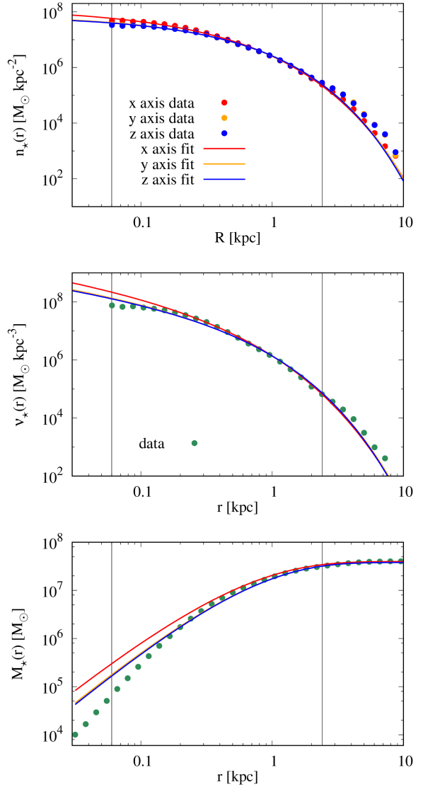
Figure 2: Top panel: the surface mass density of stars as a function of projected radius from the centre of the galaxy. Points indicate the measurements from the simulation whereas solid lines present the best-fitting Sérsic profiles. Colours denote the observations along different principal axes of the stellar component of the galaxy: red, orange and blue for the longest, intermediate and shortest axis, respectively. Middle and bottom panels: the density and cumulative mass of stars as a function of radius from the centre of the galaxy. Green dots indicate the measurements from the simulation whereas the solid lines present the analytical formulae with the parameters of the best-fitting profiles. Vertical lines mark the range in which the profiles were fitted.

We express the kinematics of a dataset in terms of proper moments of the line-of-sight velocity: the second ($m_{2}$), third ($m_{3}$) and fourth ($m_{4}$), calculated with estimators based on the sample of $N$ line-of-sight velocity measurements $v_{i}$ (Łokas & Mamon, 2003):

$$m_{n,l}=\frac{1}{N_{l}}\sum_{i=0}^{N_{l}}(v_{i}^{l}-\bar{v_{l}})^{n},$$ (8)

where

$$\bar{v_{l}}=\frac{1}{N_{l}}\sum_{i=0}^{N_{l}}v_{i}^{l}$$ (9)

and $l$ labels the radial bins. We present the profiles of the moments derived in 30 radial bins from all stellar particles in Fig. 3 in the second, third and fourth panel. Colours denote the line of sight. The top panel shows the fraction of stars in a given bin, which will be also needed for the modelling.

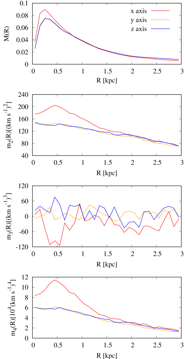
Figure 3: The fraction of the stellar mass projected along the line of sight and the 2nd, 3rd, and 4th velocity moments (top to bottom panels, respectively) derived from all stellar particles for the observations along the longest (red), intermediate (orange) and shortest (blue) principal axis.

As both the density profiles and kinematics of the datasets for the observations along the intermediate and shortest axis are almost identical, we decided to study only two lines of sight: along the longest axis $x$ and the shortest $z$.

4 Modelling large datasets

In this section we shortly describe our modelling method and its application to the mock data obtained by observing a spheroidal remnant of a major merger simulation along different lines of sight. Our datasets are presented in Sec. 3. We examined the accuracy of the recovered mass and orbit anisotropy profiles for observations along the longest and shortest principal axis in order to determine the bias caused by the non-sphericity of the tracer.

We adopted the definition of the orbit anisotropy of stars given with the anisotropy parameter (Binney & Tremaine, 2008):

$$\beta(r)=1-\frac{\sigma_{\theta}^{2}(r)+\sigma_{\phi}^{2}(r)}{2\sigma_{r}^{2}(r)}$$ (10)

where $\sigma_{r,\,\theta,\,\phi}$ are the components of the velocity dispersion in the spherical coordinate system with the origin at the centre of the galaxy. In spite of the axisymmetric shape of the galaxy, we have confirmed that the measured profile does not depend on the orientation of the adopted spherical coordinate system. Throughout the paper we will compare the results of the modelling to this real anisotropy.

4.1 Methodology

In this study we model the ratio of the total density distribution (of stars and dark matter) to the stellar density with the mass-to-light ratio varying with radius from the centre of a galaxy:

$$\Upsilon(r)=\frac{\nu_{tot}(r)}{{\nu}_{\star}(r)},$$ (11)

where $\nu_{tot}(r)$ is the total mass density and ${\nu}_{\star}(r)$ is the stellar mass density. As both quantities are given in M_☉ kpc^-3, $\Upsilon(r)$ is dimensionless. However, assigning a typical mass-to-light ratio of 1 M_☉/L_☉ to the stellar component, $\Upsilon(r)$ can be expressed in solar units, as is typically done in comparisons with observations.

We present the comparison of density profiles of stars and dark matter in the top panel of Fig. 4 with cyan and purple lines, respectively. The dark matter halo is much more extended and up to $\sim 20$ kpc can be well approximated with an NFW profile with the virial mass $M_{v,rem}=1.39\times 10^{9}$ M_☉ and the concentration $c_{rem}=21.8$. We also reproduce here the best-fitting Sérsic profiles for the two studied lines of sight in red and blue as in the bottom panel we show the profiles of mass-to-light ratio under an assumption that the stellar density follows the deprojected Sérsic profiles. As they depend on the parameters of a Sérsic profile, they depend also on the line of sight. We compare the profiles with the real mass-to-light ratio from the simulation, shown in green, which is additionally affected by a tail in the stellar distribution.

We decided to use the deprojection instead of the fit to the 3-dimensional density profile in order to avoid introducing additional parameters when the mass-to-light ratio is not known a priori. As shown in Fig. 4 the deprojections reproduce the real profile well in the considered radial range (between the vertical lines), but in the centre of the galaxy the density is overestimated. However, a core in the stellar distribution may not be of any physical nature as it appears within a radius corresponding to 3 softening scales for the dark matter particles, rather suggesting a numerical artifact.

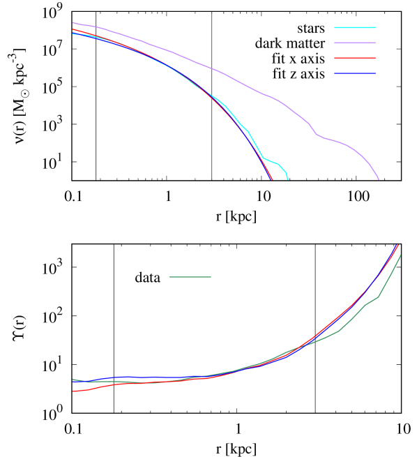
Figure 4: Top panel: the comparison of density profiles of stars (cyan line) and dark matter (purple line). Additionally, in red and blue we show the deprojected Sérsic profiles derived for the parameters of the best-fitting surface mass density profiles for observations along the longest and shortest axis. Black vertical lines mark the 3 softening scales for the dark matter and the outer radius of the data sets (from left to right, respectively). Bottom panel: the ratio between the total mass density (stars and dark matter) and stellar mass density as a function of radius. The green line presents the true values whereas the red and blue lines indicate the same ratio under the assumption that the stellar densities are given with the best-fitting Sérsic profiles.

We modelled our data by applying the spherically symmetric Schwarzschild orbit superposition method (Schwarzschild, 1979). We described and justified the details of our approach and tested its reliability in recovering the anisotropy and total mass profiles for spherical objects in Kowalczyk et al. (2017). Therefore, in this work we summarize only the crucial steps of the method:

1. For a given total density profile we generate a set of initial conditions for an orbit library. In order to properly sample orbits available in this potential, a library needs to be representative in energy and angular momentum spaces. We use 100 values of energy in units of the radius of the circular orbit sampled logarithmically and 12 values of the relative angular momentum $l=L/L_{\rm max}$, where $L_{\rm max}$ is the angular momentum of the circular orbit, sampled linearly within the open interval $l\in(0,1)$ to avoid numerical errors. Additionally, a library needs to spatially cover over 99.9% of the mass of a tracer (based on a fitted Sérsic profile) which puts a lower limit on the outer radius of a library and therefore the maximum value of energy. The minimum value is chosen so that the apocentres of corresponding orbits are smaller than the outer radius of the innermost bin used in modelling. We integrate orbits using $N$-body code GADGET-2 (Springel, 2005) saving 2001 outputs in equal timesteps with the total integration time adjusted to cover at least few orbital periods.

2. We randomly rotate each coplanar orbit 100 000 times around two axes of the simulation box, combining them to mimic the spherical symmetry and observe each orbit along an arbitrarily chosen line of sight saving the same observables in the same radial binning as for the data (see Sec. 3). Additionally, we store three components of velocity dispersion in the spherical coordinate system and deprojected fractions of mass, i.e. fractions in 3-dimensional shells. For orbits we identify the fraction of mass (projected and deprojected) in a given bin as the fraction of the total integration time spent in the bin.

3. We fit the observables of an orbit library to the data by assigning non-negative weights $\gamma$ to orbits so that their linear combination minimizes the objective function $\chi^{2}$:

   $$\chi^{2}=\sum_{l}\sum_{n}\Bigg{(}\frac{M_{l}^{\rm obs}m_{n,l}^{\rm obs}-\sum_{k}\gamma_{k}M_{l}^{k}m_{n,l}^{k}}{\Delta(M_{l}^{\rm obs}m_{n,l}^{\rm obs})}\Bigg{)}^{2}$$ (12)

   under the constraints that for each orbit $k$ and each bin $l$:

   $$\left\{\begin{array}[]{l}|M_{l}^{\rm obs}-\sum_{k}\gamma_{k}M_{l}^{k}|\leq\Delta M_{l}^{\rm obs}\\ \gamma_{k}\geq 0\\ \sum_{k}\gamma_{k}=1\end{array}\right.$$ (13)

   where $M_{l}^{k}$, $M_{l}^{\rm obs}$ are the fractions of the projected mass of the tracer contained within $l$th bin for $k$th orbit or from the observations and $m_{n,l}^{k}$, $m_{n,l}^{\rm obs}$ are $n$th proper moments. $\Delta$ denotes the measurement uncertainty associated with a given parameter. The velocity moments are weighted with the projected masses and to derive the errors we treat both quantities as independent. We execute the $\chi^{2}$ fitting of eq. (12) with rigid constraints of eq. (13) with the non-negative quadratic programming (QP) implemented in the CGAL library (The CGAL Project, 2015).

4. We derive the anisotropy resulting from the modelling assuming that the velocity dispersions in the spherical coordinate system are also given with the linear combinations of orbital dispersions weighted with the 3-dimensional mass fractions. Therefore the anisotropy in $l$th bin is:

   $$\beta_{l}=1-\frac{\sum_{k}\gamma_{k}M_{{3D},l}^{k}(\sigma_{\theta,l}^{k})^{2}+\sum_{k}\gamma_{k}M_{{3D},l}^{k}(\sigma_{\phi,l}^{k})^{2}}{2\sum_{k}\gamma_{k}M_{{3D},l}^{k}(\sigma_{r,l}^{k})^{2}}$$ (14)

   where $\sigma^{k}_{(r,\,\theta,\,\phi),l}$ are the components of the velocity dispersion for the $k$th orbit calculated in the $l$th spatial bin. We consider only $l>1$ as the result in the innermost bin cannot be trusted.

5. The best-fitting total density profile is determined as the minimum among the absolute values of $\chi^{2}$ function on a grid of density profiles created by varying the free parameters of the profile and for each of their combinations repeating steps 1-13.

   The confidence levels for the recovered density profile with two free parameters (in this work we use $a$ and $\Upsilon_{0}$, see Sec. 4.3) are derived by fitting surfaces of 4th or 8th order to the $\chi^{2}$ maps ($\sim a^{2}\Upsilon_{0}^{2}$ or $\sim a^{4}\Upsilon_{0}^{4}$ depending on the level of complexity of the map) and applying standard $\chi^{2}$ statistics for two degrees of freedom, i.e. $\Delta\chi^{2}=\chi^{2}-\chi_{min}^{2}=2.30,\,6.17,\,11.80$ corresponding to 1, 2, 3 $\sigma$ (Press et al., 1992). Fitting of a surface is necessary due to numerical artifacts affecting the method (see Kowalczyk et al. 2017 for details).

Throughout the paper we will refer to the values of various parameters obtained from the full 6D data from the simulation as real and those obtained with the modelling of mock data with the Schwarzschild method as derived.

4.2 Constant mass-to-light ratio

First, we considered the simplest scenario in which mass-follows-light, i.e. $\Upsilon(r)=\Upsilon_{0}=$ const. It is a good assumption e.g. for strongly tidally stripped galaxies orbiting their hosts on tight orbits (Łokas et al., 2013).

In this case we integrated only one orbit library for each line of sight with the total density profile matching the deprojected best-fitting Sérsic profile. Libraries for different values of $\Upsilon_{0}$, a constant scaling of mass, were obtained with a simple transformation resulting from the energy conservation and performed on each orbit separately (Rix et al., 1997):

$$v_{i} \longrightarrow \sqrt{\Upsilon_{0}}v_{i}$$ (15)

$$\bar{v_{l}} \longrightarrow \sqrt{\Upsilon_{0}}\bar{v_{l}}$$

$$m_{n,l} \longrightarrow \Upsilon_{0}^{\frac{n}{2}}m_{n,l}$$

$$\beta_{l} \longrightarrow \beta_{l}$$

where $v_{i}$ is a single line-of-sight velocity measurement on an orbit, $\bar{v_{l}}$ is the mean velocity in $l$th bin and $m_{n,l}$ is the $n$th proper moment. Since the anisotropy is defined with a ratio of velocity dispersions, the multiplication factor gets cancelled. Therefore, the transformation of the velocity dispersions in the spherical coordinate system is not necessary.

We present the results of our modelling in Fig. 5. The top panel shows the $\Delta\chi^{2}=\chi^{2}-\chi^{2}_{min}$ curves as a function of mass-to-light ratio for the observations along the longest (in red) and shortest (in blue) principal axis of the stellar component. Shaded areas identify the 1 $\sigma$ confidence levels $\Delta\chi^{2}\leq 1$ for 1 degree of freedom (Press et al., 1992). The resulting total mass profiles are shown in the middle panel together with the real mass profile derived from the simulation in green. The differences in the profiles between the best-fitting models (corresponding to the minimum of each curve) and the models contained within 1 $\sigma$ are smaller than the thickness of lines in the figure. Thin vertical lines indicate 3 softening scales for dark matter particles and the outer radius of data sets from left to right, respectively.

The bottom panel of Fig. 5 presents the anisotropy profiles: resulting from the modelling and calculated from the full data from the simulation for comparison. Colours are consistent between the panels.

Since our data clearly cannot be well approximated with a mass-follows-light model, such an assumption leads to the underestimation of mass content at large radii and the derived anisotropy strongly biased towards tangential orbits. For both lines of sight the anisotropy profiles decrease with radius and the discrepancies reach $\Delta\beta\approx 2$ at $r\geq 2$ kpc.

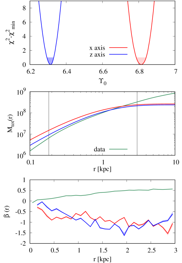
Figure 5: The results of the Schwarzschild modelling under the assumption of the mass-to-light ratio being constant with radius. Top panel: the distribution of $\Delta\chi^{2}$ as a function of mass-to-light ratio for the data based on observations along the longest (red) and shortest (blue) axis. The minima of the distributions correspond to the best-fitting models whereas the shaded ranges of the corresponding colour show 1 $\sigma$ uncertainties. Middle panel: the total mass profiles from the simulation (in green) and for the best-fitting models (red and blue lines) together with the 1 $\sigma$ error bars (shaded regions, indistinguishable in the scale of the plot). Black vertical lines mark the 3 softening scales for the dark matter and the outer radius of the data sets (from left to right, respectively). Bottom panel: the anisotropy parameter profiles. The shaded regions correspond to the extreme values for the mass-to-light ratios contained within 1 $\sigma$ confidence level.

4.3 Mass-to-light ratio varying with radius

We generalized our approach by allowing the mass-to-light ratio to vary with radius, following a formula:

$$\log\Upsilon(r)=\left\{\begin{array}[]{ll}c&\log r\leq-0.74\\ a(\log r+0.74)^{3}+c&\log r>-0.74\\ \end{array}\right.$$ (16)

where $\Upsilon(r)$ is dimensionless and $r$ is given in kpc. The parameters $a$ and $c$ are constants defining a density model.

Our formula represents a cubic curve in the log-log scale with the minimum at the radius corresponding to approximately three softening scales for the dark matter halo and constant for smaller radii. Since the case of $a=0$ reduces to the mass-follows-light model studied in the previous section, we will use $\Upsilon_{0}=10^{c}$ and we will refer to $a$ as a ‘curvature parameter’. We consider only $a\geq 0$, excluding cases where the density of the dark matter halo drops faster at large radii than the density of stars, which is not supported by any numerical experiments. Note also that our definition of the mass-to-light ratio assumes that in the centre the dark matter follows the stellar density distribution, i.e. it has the same mild cusp as the deprojected Sérsic profile.

In order to determine the true mass profiles, i.e. the combinations of parameters $a$ and $\Upsilon_{0}$ reproducing the real profiles most accurately, and quantify the bias caused only by the non-spherical shape of the galaxy, we fitted the mass-to-light ratio profiles to the full data from the simulation under the assumption that the stellar density profiles follow the deprojected best-fitting Sérsic distribution. The reason we use the deprojected best-fitting Sérsic for each line of sight is because that is what is actually observable. The deprojections are different and this difference propagates into the estimate of $\Upsilon$.

The best-fitting mass-to-light ratio profiles (‘true profiles’ hereafter) given with eq. (16) are presented in the top panel of Fig. 6 with solid lines for the observations along the longest (in red) and shortest (in blue) principal axis. Dashed lines show the real profiles from the simulation for comparison (see Fig. 4). Thin vertical lines indicate 3 softening scales for dark matter particles and the outer radius of data sets from left to right, respectively. Middle panels of Fig. 6 show the mass density and cumulative mass profiles resulting from the true mass-to-light ratio profiles and we compare them with the real profiles from the simulation (in green).

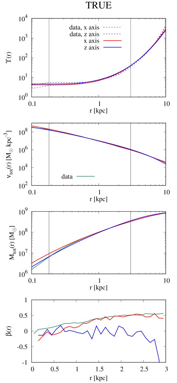
Figure 6: Results of Schwarzschild modelling for all particles under the assumption of the best-fitting mass-to-light ratio models presented in the top panel with solid lines: red for the observations along the longest and blue for the shortest principal axis. Dashed lines indicate the real profiles from the simulation under the assumption that the stellar distribution is given with the best-fitting Sérsic profiles. Black vertical lines mark the 3 softening scales for the dark matter and the outer radius of the data sets (from left to right, respectively). Second, third and forth panels: profiles of total density, cumulative total mass and anisotropy, respectively. Green lines present the real values from the simulation.

In the bottom panel we present the anisotropy profiles resulting from the modelling for the datasets obtained by observations along the longest and shortest axis in red and blue, respectively, whereas the green curve shows the real anisotropy profile of the simulated galaxy calculated from the full 6D information. For the observations along the longest axis anisotropy is underestimated only in the centre of the galaxy, where our mass-to-light ratio model overestimates cumulative mass, but is well recovered at larger radii.

The situation is much worse for the observations along the shortest axis where the derived anisotropy is approximately 0 up to $r\approx 2$ kpc and drops rapidly beyond whereas the real anisotropy profile is monotonically growing. This is an effect of the elongated shape of the galaxy in projection. Since we calculate the density and kinematics in concentric rings, we average the properties of stars which in axisymmetric modelling would belong to different elliptical shells. Therefore, we can see that even for the correct mass profile, the bias is significant.

4.4 Recovering mass-to-light ratio profile

In the next step we determined the reliability of recovering the total density and anisotropy profiles simultaneously. For this purpose we calculated two sets of orbit libraries (one for each line of sight) by varying the curvature parameter in the range $a\in[0,\,0.9]$ with a step $\Delta a=0.02$. Libraries for different values of $\Upsilon_{0}$ were obtained using the transformation given with eq. (15). We present the colour maps of the absolute values of the $\chi^{2}$ function for best-fitting models (relative to the minimum of fitted surface, see Sec. 4.1) in Fig. 7 where the top panel corresponds to the results for the observations along the longest axis whereas the bottom panel for the shortest. In both panels the true profile is marked with a green dot while the minimum of the fitted surface with a yellow one. We identify the best-fitting density model as the profile on the grid closest to the global minimum along the contours of equal $\Delta\chi^{2}$. Those models are marked with magenta dots. Additionally, with white curves we indicate the 1, 2, 3 $\sigma$ confidence levels. For the observations along the shortest axis the true profile was recovered within 2 $\sigma$, whereas for the longest axis the true profile was not recovered at all (the true profile is far outside 3 $\sigma$ contour, $\Delta\chi^{2}$>3 800). As the interpretation of bias based on the mass-to-light ratio profile parameters is difficult, we will comment on it when referring to the total mass profile.

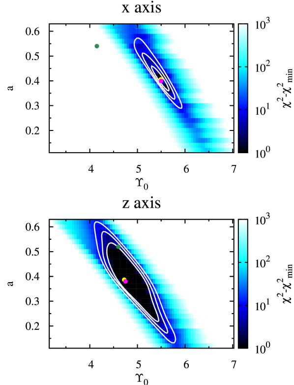
Figure 7: The maps of the $\chi^{2}$ values relative to the minima of fitted surfaces for the data sets obtained by observing the galaxy along the longest (top panel) and shortest (bottom panel) principal axis on the grids of different mass-to-light ratio models. The global minima are marked with yellow dots and the true values with green ones. Magenta points indicate the best-fitting mass profiles, i.e. the profiles on the grid closest to the global minima along the contours of equal $\Delta\chi^{2}$ plotted with white curves.

The profiles of obtained mass-to-light ratio, total density, total mass and anisotropy are presented in the consecutive panels of Fig. 8. Values for the best-fitting models (magenta dots in Fig. 7) are shown with solid lines: red for the observations along the longest principal axis and blue for the shortest. The ranges spanned by all the models contained within 1 $\sigma$ are indicated with light red and light blue shaded areas (or purple when red and blue areas overlap). In each panel the resulting parameters are compared with the real values from the simulation represented with dashed lines (mass-to-light ratio profiles only) or green solid lines (otherwise).

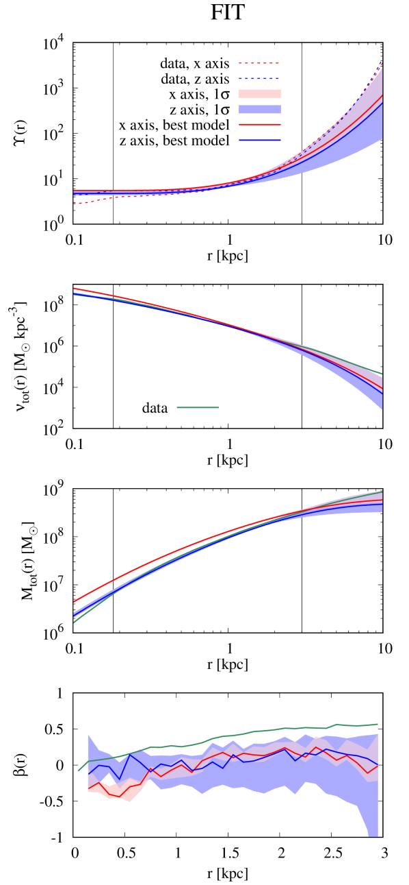
Figure 8: Results of Schwarzschild modelling for all stars based on the fitted mass-to-light ratio profiles First panel: Mass-to-light ratio profiles for the observations along the longest (red) and shortest (blue) principal axis. Dashed lines indicate the real profiles from the simulation under the assumption that the stellar distribution is given by the best-fitting Sérsic profiles whereas solid lines present the results for the best-fitting models. Shaded regions denote the spread of values for the models derived within 1 $\sigma$ confidence level. Black vertical lines mark the 3 softening scales for the dark matter and the outer radius of the data sets (from left to right, respectively). Second, third and fourth panel: profiles of total density, cumulative total mass and anisotropy, respectively. Green lines present the real values from the simulation.

The mass profile is fairly well recovered for the observations along the shortest axis and overestimated for the longest. At the outskirts of the galaxy ($r>2$ kpc) the best-fitting models for both lines of sight underestimate the mass content, however the real profile is enclosed within 1 $\sigma$.

When the density profile is to be recovered with the method, the bias in the anisotropy occurs for both lines of sight. For the observations along the longest axis the derived anisotropy profile is growing (for the best-fitting model it has a local maximum and slightly decreases at larger radii), however the values of anisotropy are systematically underestimated with the mean offset of $\Delta\beta=0.38$ for the best-fitting model. For the observations along the shortest axis the best-fitting model is consistent with isotropic orbits ($\bar{\beta}=0.08$) but 1 $\sigma$ confidence level allows the anisotropy profile to grow (with mean minimal offset with respect to the true values $\Delta\beta\approx 0.1$) or decrease (as for the true mass-to-light ratio profile).

5 Small data samples

In this part of our work we studied the bias in the recovered density and anisotropy profiles caused by the axisymmetric shape of the galaxy when the data samples used in the modelling are comparable in size with the available data sets for dwarf galaxies of the Local Group.

5.1 Examples of data modelling

We present the results of modelling for two small data samples. They were obtained by observing the remnant of the major merger simulation along the longest and shortest principal axis of the stellar component (see Sec. 3) and randomly choosing 100 000 stars for which only the projected distances from the centre of the galaxy were known and 2 500 stars with the projected distances and line-of-sight velocities. This means that the sampling follows the projected light distribution. The data are then binned into bins of equal size in the projected radius to facilitate the modelling. This results in a different number of stars per bin and the data are assigned sampling errors according to this number.

Fig. 9 presents the observables for the selected small samples (points): mass fraction based on 100 000 stars and velocity moments 2-4 of line-of-sight velocities. The same parameters in the same binning derived from all stars are shown with dashed lines for comparison. Colours, as before, denote the line of sight: red for the observations along the longest axis and blue for the shortest. Error bars indicate 1 $\sigma$ sampling errors which were determined in Monte Carlo (MC) simulations. For each line of sight and each radial bin we constructed a grid of sampling errors as a function of the number of particles in a bin. For the mass fraction we assumed Poissonian errors and they are smaller than data points in Fig. 9.

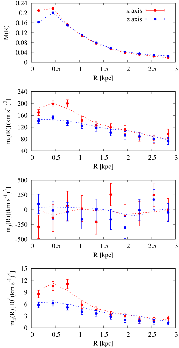
Figure 9: The fraction of the stellar mass projected along the line of sight and the 2nd, 3rd, and 4th velocity moments (top to bottom panels, respectively) for the data sets obtained by observing the galaxy along the longest (red) and shortest (blue) principal axis. The points with the 1 $\sigma$ error bars represent the values for the small random samples with sampling errors, while the thin dashed lines show the measurements based on all stellar particles from the simulations with the same binning.

The parameters of the best-fitting Sérsic profiles for the chosen subsamples of stars with distances only are quoted in Table 1 and are very similar to the ones derived for all stars. Therefore, we found it unnecessary to integrate new orbit libraries. In order to guarantee that we measure the same parameters as in Sec. 4, we assumed that the total luminosity of the galaxy and the stellar mass-to-light ratio (constant with radius) are known (Mateo 1998, McConnachie 2012).

First, we determined the sampling errors of the derived anisotropy, i.e. the uncertainties in the derived anisotropy caused by using different small samples, for the true mass-to-light ratio profiles. For that purpose for each line of sight we applied our Schwarzschild method, i.e. fitted the orbit library, to 10 000 random samples and investigated the statistics of anisotropy profiles. The values of the mean and 1 $\sigma$ deviation in each bin were obtained by fitting a Gaussian profile to the histogram of the derived anisotropy.

We present the results of this experiment in the top panel of Fig. 10 where the data points show mean values of the derived anisotropy and error bars denote 1 $\sigma$ errors. Colours indicate the line of sight: red for the observations along the longest axis and blue for the shortest. In green we reproduce the real profile of the anisotropy for comparison.

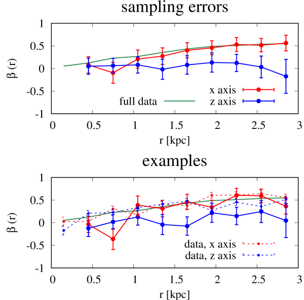
Figure 10: Top panel: Data points present the mean values of the derived anisotropy resulting from the MC simulations for the true mass-to-light ratio profiles. The red colour denotes the observations along the longest and the blue along the shortest one. The 1 $\sigma$ sampling errors are shown with error bars. The real anisotropy profile derived from the simulation is presented with a green line. Bottom panel: Examples of modelling for two small data samples (see text), one for each line of sight under the assumption of the true mass-to-light ratio profiles. Large data points connected with solid lines indicate the derived values whereas the error bars represent the 1 $\sigma$ sampling errors and are the same as in top panel. With small data points and dashed lines of the corresponding colour we show the real anisotropies calculated using only stars in small samples. For the real anisotropy the sampling errors were obtained with the MC method.

The mean values of the derived anisotropy show similar trends to those we obtained for the large samples. For observations along the longest axis the anisotropy is underestimated in the centre and well recovered at further radii. For observations along the shortest axis the anisotropy profile is consistent with an isotropic model and decreases slightly at the outskirts of the galaxy (compare with bottom panel in Fig. 6). Sampling errors for the derived anisotropy averaged over bins are 0.18 and 0.22 for the $x$ and $z$ axis, respectively.

In the bottom panel of Fig. 10 we present the anisotropy profiles (large points and solid lines) derived with our method for two random small samples, one for each line of sight, for which observables are shown in Fig. 9. We consistently use red colour for the observations along the longest axis, blue for the shortest and green for the real values (the latter calculated from all available stellar particles). The error bars are the same as in the top panel. For comparison of sampling errors between the derived and real anisotropies, values of the real anisotropy calculated from the small samples and corresponding sampling errors are shown with small points and dashed lines. As for the velocity moments, sampling errors of the real anisotropy were determined with MC simulations.

5.2 Recovering the mass profile

In the last part of our study we investigated the reliability of recovering both the mass-to-light ratio and anisotropy profiles for the two small samples described in the previous section. We used the same orbit libraries and procedures as in Sec. 4.4.

Fig. 11 presents the colour maps of $\Delta\chi^{2}$, i.e. absolute values of the objective function relative to the minimum of a fitted two dimensional surface, as a function of the two parameters of the mass-to-light ratio profile: the normalization $\Upsilon_{0}$ and the curvature parameter $a$. The two panels correspond to the different lines of sight. White loops indicate the 1, 2, 3 $\sigma$ confidence levels based on the fitted surfaces and yellow dots mark their minima. We identify the best-fitting model as the closest to the minimum on the grid of mass-to-light ratio profiles and mark them with magenta dots. Green dots show the true profiles, which were used in the previous section. Similarly to the large samples, for the observations along the shortest axis the true mass-to-light ratio profile was recovered within 1 $\sigma$ (2 $\sigma$ for large sample) and not recovered for the longest ($\Delta\chi^{2}\approx 38$).

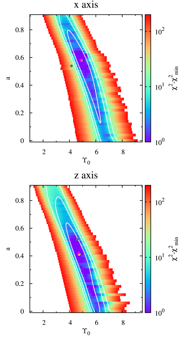
Figure 11: Maps of the $\chi^{2}$ values relative to the minima of the fitted planes for the small data samples of 100 000/2 500 stars. The two panels correspond to the data sets obtained by observing the galaxy along the longest (top) and shortest (bottom) axis. The global minima are marked with yellow dots whereas the true values of the mass-to-light ratios with green ones. Magenta dots indicate the best-fitting models identified as the closest to minimum on the grid. White lines show the contours of equal $\Delta\chi^{2}$ corresponding to 1, 2, 3$\sigma$ confidence levels.

The resulting profiles of mass-to-light ratio, total density, total mass and anisotropy are presented in consecutive panels of Fig. 12 with the solid red (for the observations along the longest axis) and blue (for the shortest) lines. Shaded areas of corresponding colours show the spread of values of a given parameter among the mass-to-light ratio models obtained within 1 $\sigma$ level (innermost loops in Fig. 11). Dashed (top panel only) and green lines (otherwise) indicate the real values from the simulation for comparison. Thin vertical lines indicate 3 softening scales for dark matter particles and the outer radius of data sets from left to right, respectively.

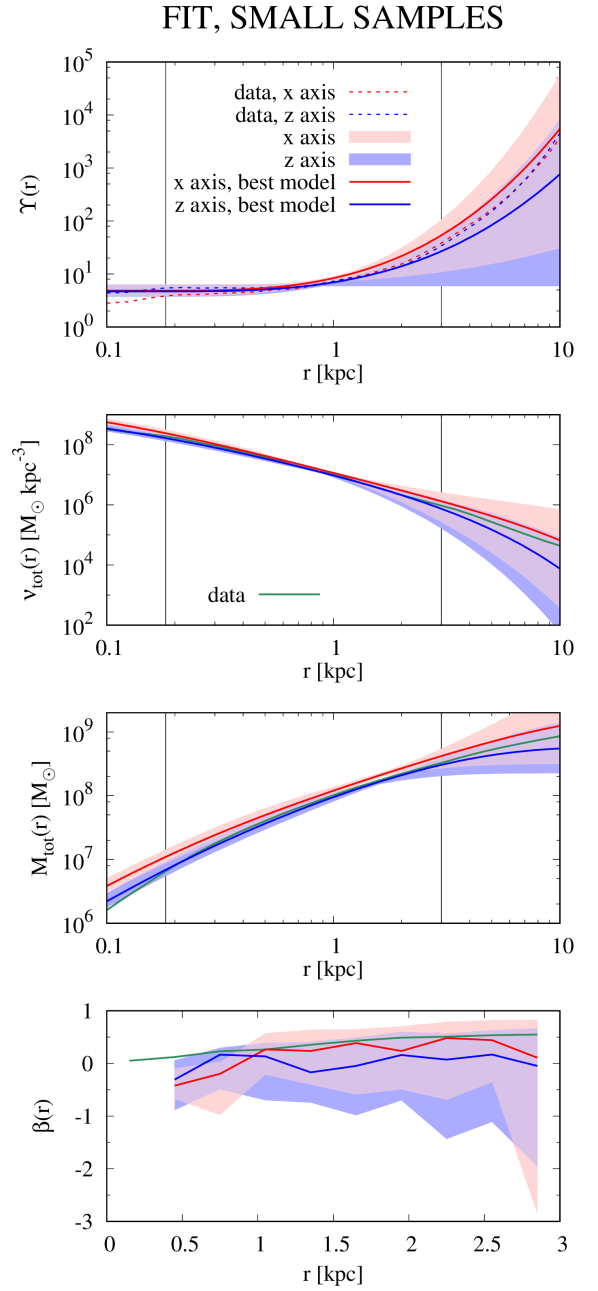
Figure 12: Same as Fig. 8 but for two small data samples, one for each line of sight.

Since the parameters of the mass-to-light ratio profile are strongly degenerated, the obtained density and mass profiles are satisfactorily well constrained up to the outer boundary of the data sets ($r_{out}=3$ kpc) and have the same bias features as for the large data samples: the mass is overestimated at all scales for the observations along the longest axis whereas for the shortest axis it is well recovered in the inner part of the galaxy but underestimated in the outer.

Also the anisotropy profiles are similar to those obtained in Sec. 4.4, however for both lines of sight 1 $\sigma$ errors are much larger and at most radii include the values of the real anisotropy. Overall, the range of derived anisotropy for the short axis observations tends to lower values, i.e. more tangential orbits are obtained in this case. Only for the observations along the longest axis the anisotropy can be significantly overestimated as shown by a larger extension of the light red region towards more radial anisotropy values.

Although for small samples the real values of anisotropy are recovered within 1 $\sigma$ confidence level, in contrast to large samples, it does not imply that in this case the anisotropy can be recovered more accurately. In fact, rather the opposite is true: the input data come with larger sampling errors so the results for small samples are less precise which allowed for the 1 $\sigma$ confidence level to contain the real values.

6 Summary and discussion

We studied the systematic errors in the recovered total mass and anisotropy profiles caused by the ellipticity of a dSph galaxy when using spherically symmetric Schwarzschild modelling method. Although ultimately models with less symmetry are expected to work better they introduce additional parameters that we believe cannot be constrained with the presently available data.

For the purpose of the tests we ran a simulation of a major merger of two identical dwarf galaxies, initially composed of an exponential stellar disc and an NFW-like dark matter halo. The stellar component of the merger remnant had an axisymmetric prolate shape with the ratio of the shortest to longest principal axis $c/a=0.84$ (or the ellipticity $\epsilon=1-c/a=0.16$). By observing our remnant along the shortest and longest axis we obtained two datasets representing the extreme cases of lines of sight which allowed us to measure the maximum bias in the recovered quantities.

We focused on the determination of the maximum, instead of the mean bias as we find it more informative. Investigating the ‘worst-case scenarios’, one may expect the results for any other line of sight to lie in between whereas averaging over many lines of sight would rather prove (or disprove) the reliability of a method for spherical objects. Since in Kowalczyk et al. (2017) we have shown that the applied method works well for spherically symmetric distribution of stars, the results presented here are particularly interesting as even for the large data samples the anisotropy is systematically underestimated and mostly consistent between the extreme lines of sight, however with different uncertainties (compare the last panel of Fig. 8 and Fig. 5 in our previous work). Therefore, we conclude that in a spheroidal galaxy for which the mass profile is unknown, independently of the amount of available data the anisotropy is not overestimated.

We modelled the total mass content with the mass-to-light ratio varying with radius from the centre of the galaxy like $\log\Upsilon(r)\sim\big{(}\log(r)\big{)}^{3}$. Such an approach is more convenient than the usual assumption of two independent components for at least two reasons. First, stars and a dark matter halo are modelled together so that any possible errors in the deprojection of the stellar distribution can be compensated. Second, the formula does not impose any particular form of the dark matter density profile, therefore comparisons between different profiles introduced in the literature (Einasto 1965, Hernquist 1990, Burkert 1995, Navarro et al. 1997) are not necessary. Additionally, the dark matter halo is naturally cut off (by the exponential drop in the stellar distribution) which is not the case e.g. for the NFW profile. Although it is customary to insert a cut-off by hand, a scale and functional form of it may influence the modelling and introduce more free parameters if an orbit library reaches the radii of that sharp drop in dark matter density.

Following the approach already applied in Kowalczyk et al. (2017), we focused on two types of data samples which we labelled ‘large’ (all stellar particles from the simulation, i.e. $4\times 10^{5}$ particles) and ‘small’ ($1\times 10^{5}$ particles with positions projected along the line of sight and 2 500 line-of-sight velocity measurements). For each type of data we divided the study into additional two steps: modelling the mock data under the assumption of the known total density profile to derive the anisotropy profile only and recovering both the anisotropy and the density profile by comparing the absolute values of the objective function.

Our results show that:

1. modelling the galaxy under the assumption that ‘mass follows light’, i.e. that the spatial distribution of the total mass can be expressed by rescaling the distribution of the visible tracer, leads to a severe inaccuracy of the resulting mass profile (overestimated in the inner parts of the galaxy and underestimated in the outskirts) and underestimation of the anisotropy parameter at all scales regardless of the line of sight;

2. if we assume that the true mass-to-light ratio profile is known the anisotropy is slightly underestimated in the centre and well recovered at larger radii for observations along the longest axis, with the accuracy similar to the spherical cases which we studied before, whereas for the shortest axis the profile is consistent with the one constant with radius and close to $\beta=0$ with sharp drop at the outskirts of the galaxy;

3. when the mass-to-light profile is to be derived, for the observations along the longest axis the total mass is overestimated (up to the outer radius of the data set) and the anisotropy is underestimated, however the general growing shape of the anisotropy profile is reproduced; for the shortest axis the mass profile is well recovered but the anisotropy is constant or decreasing with radius; for both lines of sight the mass content at large radii is recovered within 1 $\sigma$ confidence level, therefore, the method seems to be sensitive enough to determine the existence of the extended dark matter halo even if the outskirts of the galaxy do not enter the modelling;

4. when considering small data samples and the true mass-to-light ratio profiles, the mean values of the derived anisotropy averaged over many different random samples show the same trends as the results obtained for the large samples; sampling errors of the derived anisotropy are $\sim 3$ times larger than sampling errors of the real anisotropy;

5. the derivation of the mass-to-light ratio profiles for two small samples confirms the results obtained for the large ones, however the uncertainties are larger.

In summary, for prolate dSph galaxies (expected to be the most typical shape based on the currently preferred formation models) the determination of velocity anisotropy and total mass depends quite strongly on the viewing angle. If the projected shape is circular the Schwarzschild method yields an overestimate of the total mass. If the projected shape of the dSph is elongated the mass is well recovered. In both cases the anisotropy is generally underestimated, but more so in the latter. This is understandable as in a prolate spheroidal system a large fraction of the orbits are elongated along the long axis and the system has the largest velocity dispersion along this axis (see Fig. 1).

Studies of dwarf galaxies in the Local Group based on Jeans modelling often result in close to zero or negative values of anisotropy assumed to be constant with radius (Łokas et al. 2005, Łokas 2009, Walker et al. 2009). Our work shows that it is not unexpected. The simultaneous recovering of the mass and anisotropy profiles results in the flat anisotropy profiles with negative mean values.

Jardel & Gebhardt (2012) who modelled the Fornax dSph with axisymmetric Schwarzschild method based on the full line-of-sight velocity profile (while we used only moments), though assuming the orientation of the galaxy, reported opposite results. The Fornax dSph agrees well with our mock data as it is elongated, shows traces of a major merger about 6 Gyr ago (, del Pino et al.2015) with no strong interaction with Milky Way due to its extended orbit (Battaglia et al., 2015) and its data sample is similar in size. Jardel & Gebhardt (2012) recovered the profile of $\sigma_{r}/\sigma_{t}=(\beta-1)^{-1/2}$ which is mostly constant, close to 1 in the centre and rises to 1.5 at larger radii ($\beta$ rising from 0 to 0.5). Such a profile is consistent with our findings for the true mass-to-light ratio profile and observations along the longest axis. It may mean that their treatment of the elliptical projected shape of the galaxy lifted the bias. However, they also fitted the dark matter halo profile. In this case for small samples we were able to recover the true profile of anisotropy within 1 $\sigma$ confidence level but our uncertainties were much larger than shown by Jardel & Gebhardt (2012).

In contrast to other authors applying the Schwarzschild method to dwarf galaxies (Jardel & Gebhardt 2012, Jardel et al. 2013, Breddels et al. 2013, Breddels & Helmi 2013) we did not attempt to recover the inner profile of the dark matter halo. The inner profile is poorly constrained as it affects only the kinematics of stars in the very centre of the galaxy, ultimately requiring large amount of data in this region. Unfortunately, current observational data do not seem sufficient for this purpose. Our realistic small data samples presented in Sec. 5 cover a potential dark matter core with only 1-2 data points with large error bars. Therefore, with such a general method as Schwarzschild modelling deviations caused by a dark matter core would be comparable to uncertainties. However, a test of the ability of the method to recover the inner slope using large data samples might be interesting and give some insight on future developments in solving the ‘cusp-core’ problem.

We conclude that the spherical Schwarzschild modelling method proves to be useful also when applied to non-idealized, spheroidal objects created by a collision of galaxies. It is able to provide us with good estimates of the mass profile also at large radii and (at least) the lower limit on the anisotropy.

References

- Battaglia et al. (2015) Battaglia G., Sollima A., Nipoti C., 2015, MNRAS, 454, 2401
- Binney & Mamon (1982) Binney J., Mamon G. A., 1982, MNRAS, 200, 361
- Binney & Tremaine (2008) Binney J., Tremaine S., 2008, Galactic Dynamics, 2 edn. Princeton University Press, Princeton, NJ
- Breddels & Helmi (2013) Breddels M. A., Helmi A., 2013, A&A, 558, A35
- Breddels et al. (2013) Breddels M. A., Helmi A., van den Bosch R. C. E., van de Ven G., Battaglia G., 2013, MNRAS, 433, 3173
- Burkert (1995) Burkert A., 1995, ApJ, 447, L25
- Campbell et al. (2017) Campbell D. J. R. et al., 2017, MNRAS, 469, 2335
- Cappellari et al. (2006) Cappellari M. et al., 2006, MNRAS, 366, 1126
- Cretton & Emsellem (2004) Cretton N., Emsellem E., 2004, MNRAS, 327, L31
- Cretton et al. (1999) Cretton N., van den Bosch R. C. E., Frank C., 1999, ApJ, 514, 704
- Ebrová & Łokas (2015) Ebrová I., Łokas E. L., 2015, MNRAS, 394, L102
- Einasto (1965) Einasto J., 1965, Trudy Astrofizicheskogo Instituta Alma-Ata, 5, 87
- Gebhardt et al. (2003) Gebhardt K. et al., 2003, ApJ, 583, 92
- Gilmore et al. (2007) Gilmore G., Wilkinson M. I., Wyse R. F. G., Kleyna J. T., Koch A., Evans N. W., 2007, ApJ, 663, 948
- Governato et al. (2010) Governato F. et al., 2010, Nature, 463, 203
- Hernquist (1990) Hernquist L., 1990, ApJ, 356, 359
- Jardel & Gebhardt (2012) Jardel J. R., Gebhardt K., 2012, ApJ, 746, 89
- Jardel et al. (2013) Jardel J. R., Gebhardt K., Fabricius M. H., Drory N., Williams M. J., 2013, ApJ, 763, 91
- Kazantzidis et al. (2011a) Kazantzidis S., Łokas E. L., Callegari S., Mayer L., Moustakas L. A., 2011a, ApJ, 726, 98