Emergence, evolution, and control of multistability in a hybrid topological quantum/classical system

Abstract

We present a novel class of nonlinear dynamical systems - a hybrid of relativistic quantum and classical systems, and demonstrate that multistability is ubiquitous. A representative setting is coupled systems of a topological insulator and an insulating ferromagnet, where the former possesses an insulating bulk with topologically protected, dissipationless, and conducting surface electronic states governed by the relativistic quantum Dirac Hamiltonian and latter is described by the nonlinear classical evolution of its magnetization vector. The interactions between the two are essentially the spin transfer torque from the topological insulator to the ferromagnet and the local proximity induced exchange coupling in the opposite direction. The hybrid system exhibits a rich variety of nonlinear dynamical phenomena besides multistability such as bifurcations, chaos, and phase synchronization. The degree of multistability can be controlled by an external voltage. In the case of two coexisting states, the system is effectively binary, opening a door to exploitation for developing spintronic memory devices. Because of the dissipationless and spin-momentum locking nature of the surface currents of the topological insulator, little power is needed for generating a significant current, making the system appealing for potential applications in next generation of low power memory devices.

Topological quantum materials are a frontier area in condensed matter physics and material sciences. A representative class of such materials is topological insulators, which have an insulating bulk but possess dissipationless conducting electronic states on the surface. For a three-dimensional topological insulator (3D TI) such as Bi₂Se₃, the surface states have a topological origin with a perfect spin-momentum locking, effectively eliminating backscattering from non-magnetic impurities and generating electronic “highways” with highly efficient transport. The surface states can generally be described by a two-dimensional Dirac Hamiltonian in relativistic quantum mechanics. When a piece of insulating, ferromagnetic material is placed on top of a topological insulator, two things can happen. Firstly, there is a spin-transfer torque from the spin-polarized surface current of the topological insulator to the ferromagnet, modulating its magnetization and making it evolve dynamically. Secondly, the ferromagnet generates an exchange coupling to the Hamiltonian of the topological insulator, reducing its quantum transmission from unity and rendering it time dependent. Due to these two distinct types of interactions in the opposite directions, the coupled system of topological insulator and ferromagnet constitutes a novel class of nonlinear dynamical systems - a hybrid type of systems where a relativistic quantum description of the surface states of the 3D TI and a classical modeling of the ferromagnet based on the LLG (Landau-Lifshitz-Gilbert) equation are necessary. The hybrid dynamical system can exhibit a rich variety of nonlinear dynamical phenomena and has potential applications in spintronics. Here we review some recent results in the study of such systems, focusing on multistability. In particular, we demonstrate that multistability can emerge in open parameter regions and is therefore ubiquitous in the hybrid relativistic quantum/classical systems. The degree of multistability as characterized by the ratio of the basin volumes of the multiple coexisting states can be externally controlled (e.g., by systematically varying the driving frequency of the external voltage). The controlled multistability is effectively switchable binary states that can be exploited for developing spintronic memory. For example, in spintronics, the multiple stable states of the magnetization are essential for realizing efficient switching and information storage (e.g., magnetoresistive random-access memory - MRAM, with a read-out mechanism based on the giant magnetoresistance effect). MRAM is widely considered to be the next generation of the universal memory after the current FLASH memory devices. A key challenge of the current MRAM technology lies in its significant power consumption necessary for writing or changing the direction of the magnetization. The spin-transfer torque based magnetic tunnel junction configuration has been developed for power-efficient MRAMs. For this type of applications the coupled TI-ferromagnet system represents a paradigmatic setting where only extremely low driving power is needed for high performance because of the dissipationless nature of the spin-polarized surface currents of the TI.

I Introduction

The demands for ever increasing processing speed and diminishing power consumption have resulted in the conceptualization and emergence of physical systems that involve topological quantum states. Such a system can appear in a hybrid form: one component effectively obeying quantum mechanics on a relatively large length scale ($\sim\mu$m) while another governed by classical or semiclassical equations of motion, with interactions of distinct physical origin in opposite directions. The topological states based quantum component acts as an electronic highway, where electrons can sustain a dissipationless, spin-polarized current under a small electrical driving field. The dynamics of the classical component can be nonlinear, leading to a novel class of nonlinear dynamical systems. We believe such systems represent a new paradigm for research on nonlinear dynamics. The purpose of this mini-review article is to introduce a class of coupled topological quantum/classical hybrid systems, and discuss the dynamical behaviors with a special focus on the issue of multistability. Significant potential applications will also be articulated.

The practical motivations for studying the class of topological quantum/classical hybrid systems are the following. The tremendous advances of information technology relied on the development of hardwares. Before 2003, the clock speed of CPU increases exponentially as predicted by Moore’s law and Dennard scaling Sutter:2005 . As we approach the end of Moore’s law, mobile Internet rises, which requires more power efficient and reliable hardwares. Mobile Internet connects every user into the network and provides enormous data, leading to the emergence of today’s most rapidly growing technology - artificial intelligence (AI) CV:2015 ; LBH:2015 ; JM:2015 . The orders of magnitude increases in abilities to collect, store and analyze information require new physical principles, designs, and methods - “more is different” Anderson:1972 . In the technological development, quantum mechanics has become increasingly relevant and critical. In general, when the device size approaches the scale of about 10nm, quantum effects become important. In the current mesoscopic era, a hybrid systems description incorporating classical and quantum effects is essential. For example, quantum corrections such as energy quantizations and anisotropic mass are necessary in the fabrication of CMOS USK:2008 , the elementary building block of CPU and GPU. In terms of memory devices, the magnetic tunnel junction (MTJ) based spin-transfer torque random access memory (STTRAM) HYYBHYYSHF:2005 ; TKMYHMOYIT:2010 is becoming a promising complement to solid state drives, whose core is a tunnel junction design with multilayer stacks, where a layer of ferromagnetic materials with a fixed magnetization is used to polarize the spin of the injected current. As a fully quantum phenomenon, the spin polarized current tunnels through a barrier to drive the magnetization in the magnetically soft ferromagnetic layer - the so-called free layer for information storage.

The basic principles of STTRAM was proposed about two decades ago in the context of spintronics before the discovery of topological insulators (TIs) BHZ:2006 ; HK:2010 ; QZ:2011 . In addition, a current-induced spin-orbit torque mechanism GM:2011 was proposed as an alternative way to harness the magnetization of conducting magnetic or magnetically doped materials with large spin-orbit coupling. With the advance of 3D TIs, much more efficient operations are anticipated with giant spin-orbit torque and spin-transfer torque. Particularly, in comparison with the conventional spin-orbit torque settings in heavy metals with a strong Rashba type of spin-orbit coupling MGARSPVG:2010 ; MGGZCABRSG:2011 ; PWBLCKS:2010 ; WM:2012 , the spin density in 3D topological insulator based systems can be enhanced substantially by the factor $\hbar v_{F}/\alpha_{R}\gg 1$, where $v_{F}$ is the Fermi velocity in the TI and $\alpha_{R}$ is the strength of the Rashba spin-orbit coupling in two-dimensional electron gas (2DEG) systems CMSSN:2015 . The two-layer stack configurations of TI/ferromagnet DLSK:2015 ; TST:2015 ; JLJMLZNMSW:2015 or TI/anti-ferromagnet RNS:2017 ; LDSK:2017 have recently been articulated, which allow for the magnetization of the depositing magnetic materials to be controlled and the transport of spin-polarized states on the surface of the 3D TIs to be modulated.

To be concrete, in this paper we consider the ferromagnet-TI configuration and focus on the dynamics of the magnetization in the insulating ferromagnet and the two orthogonal current components on the surface of the TI: one along and another perpendicular to the direction of an externally applied electrical field. A schematic illustration of the system is presented in Fig. 1(a), where a rectangular shape of the ferromagnet is deposited on the top of a TI. For the ferromagnet, the dynamical variable is the magnetization vector ${\bf M}$, whose evolution is governed by the classical Landau-Lifshitz-Gilbert (LLG) equation Slonczewski:1996 , which is nonlinear. The TI, as will be described in Sec. II, hosts massless spin-$1/2$ quasiparticles in the low-energy regime ($\sim$meV) on its surface and generates spin polarized surface currents when a weak electrical field is applied BHZ:2006 ; HK:2010 ; QZ:2011 . In fact, the surface states of the TI are described by the Dirac Hamiltonian, rendering it effectively relativistic quantum. Physically, the interactions between TI and ferromagnet can be described, as follows. The robust spin polarized current on the surface of the TI generates MLRGMFVMKS:2014 a strong spin-transfer torque RS:2008 to the ferromagnet, inducing a change in its magnetization vector. The ferromagnet, in turn, generates a proximity induced exchange field in the TI. As a result, there is an exchange coupling term in the surface Dirac Hamiltonian of the TI, which modulates the quantum transmission and leads to a change in the surface current. The two-way interactions between the ferromagnet and TI are schematically illustrated in Fig. 1(b), where the whole coupled system is of a hybrid type: effectively relativistic quantum TI and classical ferromagnet. The interactions render time dependent the dynamical variables in both TI and ferromagnet: the surface current for the former and the magnetization vector for the latter. Due to the intrinsic and externally spin-transfer torque induced nonlinearity of the LLG equation, the whole configuration represents a nonlinear dynamical system, in which a rich variety of phenomena such as bifurcations, chaos, synchronization, and multistability can arise WXL:2016 .

Following the theme of the Focus Issue, in this paper we focus on the emergence, evolution and control of multistability. When a small external voltage with both a dc and ac component is applied to the TI, a robust spin-polarized surface current rises, as shown in Fig. 1(a). In certain open parameter regions, the magnetization can exhibit two coexisting stable states (attractors) with distinct magnetic orientations, each having a basin of attraction. As the phase space for the magnetization is a spherical surface, the basin areas of the two attractors are well defined. (This is different from typical dissipative nonlinear dynamical systems in which the basin of attraction of an attractor has an infinite phase space volume Ott:book .) As an external parameter, e.g., the frequency of the ac voltage, is varied, the relative basin areas of the two attractors can be continuously modulated. In fact, as the parameter is changed systematically, both birth and death of multistability can be demonstrated, rendering feasible manipulation or control of multistability. While some of these results have appeared recently WXL:2016 , here we focus on those that have not been published.

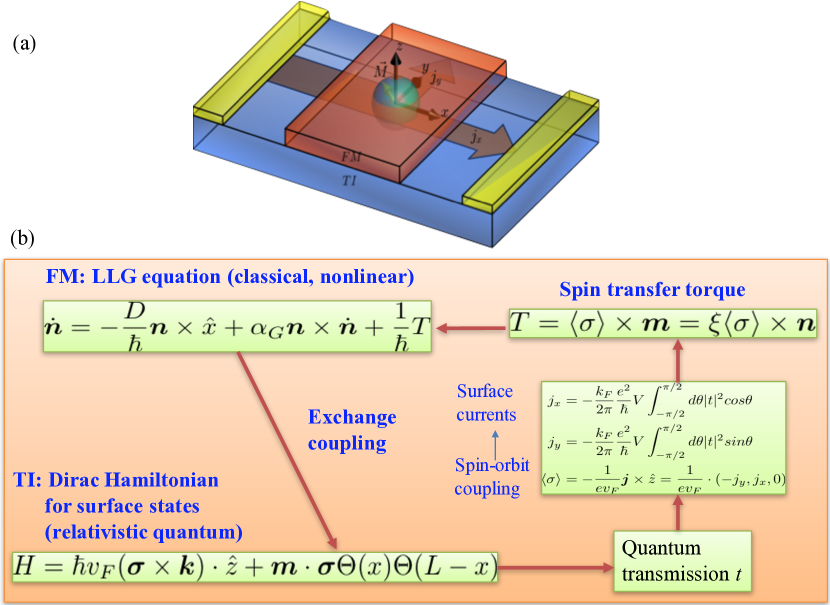
Figure 1: Schematic illustration of a representative relativistic quantum/classical hybrid system, the physical interactions, and the dynamical evolution of the states. (a) A coupled ferromagnet and topological insulator (TI) system, where the ferromagnet is deposited on the top of the TI. (b) The physical interactions: spin-transfer torque (from TI to ferromagnet) and exchange coupling (from ferromagnet to TI). The dynamical evolution of the ferromagnet is described by the classical, nonlinear LLG equation, and the dissipationless, spin-polarized surface states of the TI are determined by the Dirac Hamiltonian. Refer to Secs. II and III for the meanings of the mathematical notations and equations.

In Sec. II, we provide a concise introduction to the basics of TIs and the Dirac Hamiltonian with a focus on the physical pictures of the emergence of strong, spin-polarized surface states. In Sec. III, we describe the mechanism of spin transfer torque and the rules of the dynamical evolution of the TI-ferromagnet coupled system in terms of the LLG equation and the quantum transmission of the TI. In Sec. IV, we present results of multistability, followed by a discussion of potential applications in Sec. V.

II Topological insulators

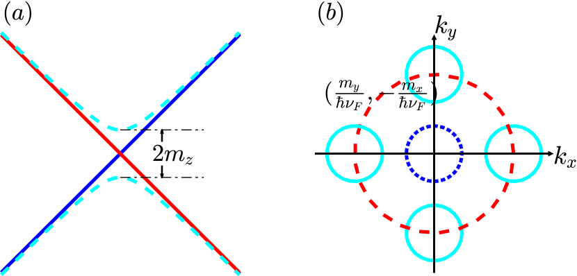
Figure 2: Surface states of topological insulators and the effect of magnetization. (a) Red and blue lines represent the linear dispersion relation of the surface states of an ideal TI without a gap opening perturbation, with the slope $\hbar\nu_{F}$. The two states have opposite spin polarizations. The presence of a perpendicular magnetization vector $m_{z}$ leads to a gap opening of size proportional to $2m_{z}$, making the dispersion relation hyperbolic. (b) Magnetization vectors in the plane of the TI, i.e., $m_{x}$ and $m_{y}$, will shift the central position of the Fermi surface in the wave vector space, inducing an asymmetry with respect to either $k_{y}=0$ or $k_{x}=0$.

One of the most remarkable breakthroughs in condensed matter physics in the last decade is the theoretical prediction BHZ:2006 ; FK:2007 ; ZLQDFZ:2009 and the subsequent experimental realization KWBRBMQZ:2007 ; HQWXHCH:2008 ; XQHWPLBGHC:2009 of TIs Moore:2010 ; HK:2010 ; QZ:2011 . TIs are one emergent phase of the material that has a bulk band gap so its interior is an insulator but with gapless surface states within the bulk band gap. The surface states are protected by the time-reversal symmetry and therefore are robust against backscattering from impurities, which are practically appealing to developing dissipationless or low-power electronics. Moreover, the surface states possess a perfect spin-momentum locking, in which the spin orientation and the direction of the momentum is invariant during the propagation.

TIs are representative of topologically protected phases of matter TKNN:1982 ; Haldane:1988 , one theme of last year’s Nobel prize NP:2016 . The prediction and experimental realization of TIs benefited from the well known quantum Hall effect KDP:1980 , also a topological quantum order. The topological phases of matter not only are of fundamental importance, but also have potential applications in electronics and spintronics PM:2012 . According to the bulk-edge correspondence in topological field theory, gapless edge states exist at the boundary between two materials with different bulk, topologically invariant numbers HK:2010 . The edge states are protected by the topological properties of the bulk band structures, and thus are extremely robust against local perturbations. Depending on the detailed system setting, there are remarkable properties associated with the edge states such as perfect conductance, uni-directional transportation, and spin-momentum coupling BHZ:2006 ; HK:2010 ; QZ:2011 .

We learned from elementary physics that a perpendicular magnetic field applied to a conductor subject to a longitudinal electrical field will induce a transverse voltage - the classic Hall effect Hall:1879 . In 1980, it was discovered that, for a 2DEG at low temperatures, under a strong magnetic field the Hall conductivity is quantized exactly at the integer multiple of the fundamental conductivity $e^{2}/h$, where $-e$ is the electronic charge and $h$ is the Planck constant. This is the integer quantum Hall effect (usually referred to as QHE) KDP:1980 . Different from the classical Hall effect, the quantized Hall conductivity is fundamentally a quantum phenomenon occurring at the macroscopic scale Laughlin:1981 . Soon after, new states of matter such as the fractional quantum Hall effect (FQHE) TSG:1982 ; Laughlin:1983 ; Nobel:1998 ; STG:1999 , quantum anomalous Hall effect (QAHE) Haldane:1988 , and the quantum spin Hall effect (QSHE) Hirsch:1999 ; MNZ:2003 ; SCNSJM:2004 ; BZ:2006 were discovered. Besides their fundamental significance, such discoveries have led to an unprecedented way to understand and explore the phases of matter through a connection of two seemingly unrelated fields: condensed matter physics and topology.

Heuristically, QHE can be understood in terms of the Landau levels - energy levels formed due to a strong magnetic field. Classically, an electron will precess under such a field. Quantum mechanically, only the orbits whose circumference is an integer multiple of $2\pi$ can emerge (constructive interference), leading to the Landau levels. QHE can be understood as a result of the Fermi level’s crossing through various Landau levels Datta:book as, e.g., the strength of the external magnetic field is increased.

At a deeper level, the robustness of the quantized conductivity in QHE can be understood as a topological effect. To understand the concept of topology in physical systems, we consider a two-dimensional closed surface characterized by a Gaussian curvature. According to the Gauss-Bonnet theorem, the number of holes associated with a compact surface without a boundary can be written as a closed surface integral:

$$4\pi(1-g)=\oiint(\mbox{Gaussian curvature})\cdot da,$$

where we have $g=0$ for a spherical surface and $g=1$ for a donut surface (a two-dimensional torus). Different types of geometrical surfaces can thus be characterized by a single number. This idea has been extended to physics with a proper definition of geometry in terms of the quantum eigenstates, where a generalized Gauss-Bonnet formula by Chern applies. In particular, consider the band structure of a 2D conductor or a 2DEG. Let $|u_{m}({\bf k})\rangle$ be the Bloch wavefunction associated with the $m$th band. The underlying Berry connection is

$${\bf A}_{m}=i\langle u_{m}({\bf k})|\nabla_{\bf k}|u_{m}({\bf k})\rangle.$$ (1)

The Berry phase is given by

$$\Phi_{B}=\oint{\bf A}_{m}\cdot d{\bf l}=\oiint(\nabla\times{\bf A}_{m})\cdot{\bf ds},$$ (2)

where ${\bf F_{m}}=\nabla\times{\bf A}_{m}$ is the Berry curvature. The total Berry flux associated with the $m$th band in the Brillouin zone is

$$n_{m}=\frac{1}{2\pi}\iint d^{2}{\bf k}\cdot{\bf F_{m}},$$ (3)

which is the Chern number TKNN:1982 ; HK:2010 . Let $N$ be the number of occupied bands. The total Chern number is

$$n=\sum^{N}_{m=1}n_{m}.$$ (4)

It was proved TKNN:1982 that the Hall conductivity is given by

$$\sigma_{xy}=n\frac{e^{2}}{h}.$$ (5)

As the magnetic field strength is increased, the integer Chern number increases, one at a time, leading to a series of plateaus in the conductivity plot. The Chern number is a topological invariant: it cannot change when the underlying Hamiltonian varies smoothly TKNN:1982 . This leads to robust quantization of the Hall conductance. Due to its topological nature and the time-reversal symmetry breaking, dissipationless chiral edge conducting channels emerge at the interface between the integer quantum Hall state and vacuum, which appears to be promising for developing low-power electronics but with the requirement of a strong external magnetic field. Nevertheless, the topological ideas developed in the context of QHE turned out to have a far-reaching impact on pursuing distinct topological phases of matter.

The QSHE represents a preliminary manifestation of TIs with a time reversal symmetry, as a 2D TI, essentially a quantum spin Hall state, was predicted in the CdTe-HgTe-CdTe quantum well system BHZ:2006 and experimentally realized KWBRBMQZ:2007 . Both CdTe and HgTe have a zinc blende crystal structure and have minimum band gaps about the $\Gamma$ point. The origins of the conduction and valance bands are $s$ and $p$ atomic orbitals. Compared with CdTe, HgTe can support an inverted band structure about the $\Gamma$ point, i.e., CdTe has an $s$-type conduction band and a $p$-type valance band while HgTe has a $p$-type conduction band and an $s$-type valance band. Mathematically, the inversion is equivalent to a change in the sign of the effective mass. The difference is in fact a result of the strong spin-orbit coupling in HgTe, which can reduce the band gap and even invert the bandstructure through orbital splitting. (In experiments, the band gap can be widened by increasing the size of the quantum confinement.) Intuitively, a CdTe-HgTe-CdTe quantum well can be thought of as making a replacement of the layers of Cd atoms by Hg. When the HgTe layer is thin, the properties of CdTe is dominant and the quantum well is in the normal regime. As one increases the thickness of the HgTe layer, eventually the configuration of the conduction and valance bands will become similar to that of HgTe so the quantum well is in the inverted regime. The interface joining the two materials with the inverted configuration acts as a domain wall and can potentially harbor novel electronic states described by a distinct Hamiltonian.

In general, regardless of the material parameters, the Hamiltonian can be written in the momentum space as $H=H(k_{x},k_{y},-i\partial_{z})$, where $z$ stands for the stacking direction so $k_{z}$ is not a good quantum number. Integrating this Hamiltonian within several dominant $z$ base states, one can arrive at an effective Hamiltonian for the 2D TI, which is characterized by $k_{x}$ and $k_{y}$. Edge states can be obtained by imposing periodic boundary conditions along one direction and open boundary conditions in another. The inverted band structure, i.e., the basis, and the time-reversal symmetry guarantee the gaplessness of the edge state while the detailed form of the open boundary plays a secondary role only. For a pedagogical review of 2D TIs, see Ref. KBWHLQZ:2008 .

Parallel to the study of 2D TIs, there were efforts in uncovering 3D TIs, for which Bi_1-xSb_x was theoretically proposed to be a candidate FK:2007 ; MNZ:2003 . The prediction was confirmed experimentally shortly after HQWXHCH:2008 . However, since Bi_1-xSb_x is an alloy with random substitutional disorders, its surface states are quite complicated, rendering difficult a description based on an effective model. The attention was then turned to finding 3D TIs in stoichiometric crystals with simple surface states, leading to the discovery XQHWPLBGHC:2009 ; ZLQDFZ:2009 of Bi₂Se₃. In particular, it was experimentally observed XQHWPLBGHC:2009 that there is a single Dirac cone on the surface of Bi₂Se₃. A low-energy effective model was then proposed ZLQDFZ:2009 for Bi₂Se₃ as a 3D TI, in which spin-orbit coupling was identified as the mechanism to invert the bands in Bi₂Se₃ and the four most relevant bands about the $\Gamma$ point were used to construct an effective bulk Hamiltonian. A generic form of the Hamiltonian was written down in the space constituting the four bases up to the order of $O(\bm{k}^{2})$, constrained by a number of symmetries: the time-reversal, the inversion, and the three-fold rotational symmetries. The parameter associated with each term was determined by fitting the dispersion relation with the ab initio computational results. The surface states can be obtained by imposing constraints along one direction, which mathematically entails replacing $k_{z}$ by $-i\partial_{z}$ while keeping the states along the other two directions oscillatory. The effective surface Hamiltonian can be calculated by projecting the bulk Hamiltonian onto the surface states. At the present, Bi₂Se₃ is one of the most commonly studied 3D TIs, which possesses gapless Dirac surface states protected by the time-reversal symmetry and a bulk band gap up to $0.3\mbox{eV}$ (equivalent to $3000\mbox{K}$ - far higher than the room temperature).

The widely used Hamiltonian for the surface states of an ideal 3D TI is

$$H=\hbar v_{F}(\bm{\sigma}\times\bm{k})\cdot\hat{z},$$ (6)

where $v_{F}$ is the Fermi velocity of the surface states ($v_{F}\approx 6.2\times 10^{5}\mbox{m}/\mbox{s}$ for Bi₂Se₃), and $\bm{\sigma}=(\sigma_{x},\sigma_{y},\sigma_{z})$ are the Pauli matrices describing the spin of the surface electron ZLQDFZ:2009 . An elementary calculation shows that the dispersion relation of this surface Hamiltonian indeed has the structure of a Dirac cone. In proximity to a ferromagnet with a magnetization $\bm{m}$, an extra term $\bm{m}\cdot\bm{\sigma}$ in the Hamiltonian (6) will be induced. Due to the breaking of the time reversal symmetry by the exchange field, gap opening for the surface states will occur and backward scatterings will no longer be forbidden. The proximity induced exchange field will thus modulate the charge transport behaviors of the surface states and the underlying spin density by disturbing the spin texture, which in turn can be a driving source of the nonlinear dynamic magnetization in the adjacent ferromagnetic cap layer through a spin-transfer torque.

III Spin-transfer torque

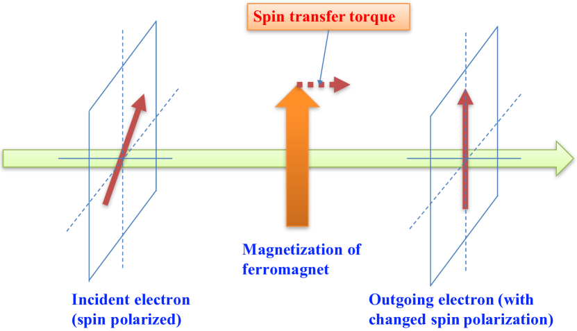
Figure 3: Schematic illustration of spin-transfer torque. The large green arrow indicates an electron flow under an external longitudinal voltage. The electrons are spin polarized (e.g., the surface states of a 3D TI). As the electrons pass through a region in which a magnetization vector is present (e.g., a ferromagnetic region), it exerts a torque on the magnetization, due to which the spin polarization of the outgoing electrons is changed, henceforth the term “spin-transfer torque.”

Spin-transfer torque RS:2008 is a major subject of research in spintronics LCG:2014 , a field aiming to understand and exploit the spin degree of freedom of electrons beyond the conventional charge degree of freedom. Intuitively, spin-transfer torque is nothing but the exchange interaction between two magnetization vectors. In particular, when two magnetization vectors are brought close to each other, they tend to align or anti-align with each other to evolve into a lower energy state. In our coupled TI-ferromagnet system, one magnetization vector is the net contribution of the spin-polarized current on the surface of the TI, and the other comes from the ferromagnet. A setting to generate a spin-transfer torque is schematically illustrated in Fig. 3. The basic physical picture can be described, as follows. When a normal current flows near or within a region in which a strong magnetization is present, the spin associated with the current will be partially polarized. This implies that, by the law of action and reaction, a spin-polarized current will exert an torque on the magnetization - the spin-transfer torque. Such a torque will induce oscillations, inversion and other dynamical behaviors of the magnetization. The ability to manipulate magnetization is critical to applications, especially in developing memory devices.

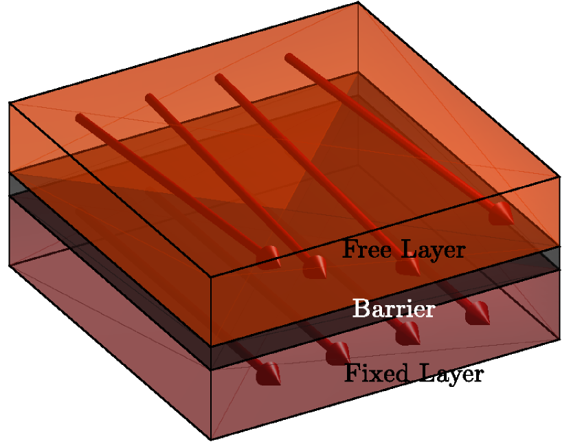
Figure 4: Schematic illustration of a magnetic tunnel junction (MTJ). A typical MTJ consists of a fixed layer, a barrier and a free layer. An electrical current is injected vertically into the fixed layer and comes out from the free layer. The average spin of the current is polarized by the fixed layer, which tunnels through the insulating barrier and drives the magnetization of the free layer. This configuration can be used to modify and detect the magnetization direction in the free layer through the giant magnetoresistance (GMR) effect.

Conventionally, a three-layer magnetic tunnel junction (MTJ) is used to study spin-transfer torque GNSTOAGHBZ:2012 ; BKO:2012 ; LCG:2014 , in which the fixed layer is a ferromagnet with a permanent magnetization. A schematic illustration of an MTJ is presented in Fig. 4. When a normal current is injected into this layer, the spin will be partially polarized due to the individual exchange interaction between each single electron spin and the magnetization. As a result, there is randomness in the polarization with no definite correlation between the direction of the electron spin and momentum. To separate the fixed from the free layer, a thin insulating separation barrier is needed to form a tunnel junction. The current will travel through the insulating barrier via the mechanism of quantum tunneling, during which the direction of spin will not be altered insofar as the insulating barrier does not have any magnetic impurity. After the tunneling, the spin-polarized current will exert a spin-transfer torque on the magnetization in the free ferromagnetic layer, modifying the information stored. Readout of the information, i.e., the direction of the magnetization, can be realized by exploiting the giant magnetoresistance effect BBFVPECFC:1988 ; BGSZ:1989 ; Nobel:2007 .

An issue with MTJ is that a very large current is needed to reorient the magnetization, motivating efforts to explore alternative mechanisms with a lower energy requirement. One mechanism was discovered in ferromagnet/heavy-metal bilayer heterostructures MGGZC:2011 ; LPLTRB:2012 . The strong Rashba spin-orbit coupling in many heavy metals can be exploited through the mechanism of spin-orbit torque to generate spin-polarized currents via the Edelstein effect, which are generally much stronger than the exchange interaction between the fixed layer and current spin in the conventional MTJ. Moreover, the current in the configuration needs no longer to be restricted to the perpendicular direction, but can have any orientation within the film plane. This new geometrical degree of freedom enables unconventional strategies for manipulating magnetization. For example, it was discovered SJLBAPBMG:2016 that the domain wall motions (essentially the dynamics of magnetization) in the covering magnetic free layer have a sensitive dependence on the spatial distribution of the current generated spin-orbit torque.

A disadvantage of the spin-orbit torque configuration is that the heavy metals usually suffer from substantial scatterings and the transportation mechanisms are complex. In addition, for heavy metals, spin-orbit coupling is essentially a higher-order effect. As a result, the currents are not perfectly polarized. These difficulties can be overcome by exploiting TIs as a replacement for heavy metals.

Mathematically, the Hamiltonian term describing the Rashba spin-orbit coupling has the same form as the effective surface Hamiltonian of a 3D TI, i.e., $\sim\bm{\sigma}\times\bm{k}$. This is basically the whole Hamiltonian for the surface states of 3D TI under the low energy approximation. The presence of an exchange field from the ferromagnetic cap layer will contribute a Zeeman term to the Hamiltonian. To see this explicitly, we consider the surface Hamiltonian of a 3D TI in the presence of a magnetization

$$\hbar v_{F}(\bm{\sigma}\times\bm{k})\cdot\hat{z}+\bm{m}\cdot\bm{\sigma}$$

$$= \hbar v_{F}[\sigma_{x}\cdot(k_{y}+\frac{m_{x}}{\hbar v_{F}})-\sigma_{y}\cdot(k_{x}-\frac{m_{y}}{\hbar v_{F}})]+m_{z}\sigma_{z},$$

where the $m_{z}$ term only induces a band gap due to the breaking of the time-reversal symmetry for the surface states. The $m_{x}$ and $m_{y}$ terms are equivalent to a shift in the center of the Fermi surface, as shown in Fig. 2(b). Consequently, the surface currents and the associated spin densities flowing through the magnetization region will be modulated. In addition, as the TI contains an insulating bulk with a band gap much larger than the room temperature thermal fluctuations, the only conducting modes are those associated with the spin-polarized surface states. The coupled TI/ferromagnet configuration has been experimentally realized MLRGMFVMKS:2014 . So far the system provides the strongest spin-transfer torque source - two to three orders of magnitude higher than that in heavy metals.

The magnetization dynamics of the ferromagnet deposited on the 3D TI can be described by the classical LLG equation Slonczewski:1996 , which captures the essential physical processes such as procession and damping of the magnetization subject to external torques. The LLG equation is

$$\dot{\bm{n}}=-\frac{D}{\hbar}\bm{n}\times\hat{x}+\alpha_{G}\bm{n}\times\dot{\bm{n}}+\frac{1}{\hbar}\bm{T},$$ (7)

where the first term represents the procession along the easy axis $\hat{x}$ and $D$ is the anisotropic energy of the ferromagnet. The second term describes the Gilbert damping of strength $\alpha_{G}$. The last term is the contribution from the external torque, which is the spin-transfer torque:

$$\bm{T}=\langle\bm{\sigma}\rangle\times\bm{m}=\xi\langle\bm{\sigma}\rangle\times\bm{n},$$ (8)

where, for convenience, we use $\xi=|\bm{m}|$ (the magnitude of the magnetization) as a normalizing factor so that $\bm{n}=\bm{m}/\xi$ becomes a unit vector.

IV Emergence, evolution and control of multistability

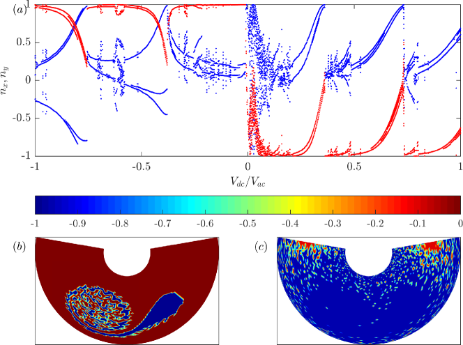
Figure 5: Bifurcations and multistability in the coupled TI-ferromagnet system. (a) A bifurcation diagram for $\Omega/\omega_{F}=7.0$, where the parameter ratio $V_{dc}/V_{ac}$ is swept from $-1.0$ to $1.0$. The system exhibits rich dynamics. In several parameter regimes, there are abrupt changes in the final states. A systematic computation with different initial conditions reveals multistability. (b-c) For $\Omega/\omega_{F}=10.0$, typical examples of multistability. The phase space of the normalized magnetization ${\bf n}$ of the ferromagnet is the surface of a unit sphere. All possible initial conditions from the spherical surface are distinguished by different colors. The Albers equal-area conic projection is used to map the initial conditions from the spherical surface to a plane while preserving the area of each final state. The standard parallels of the Albers projection are $\frac{2}{9}\pi,\frac{7}{18}\pi$. Shown are the basins of two final states.

To study the nonlinear dynamics of the coupled TI-ferromagnet system, we couple the transportation of current on the surface of TI with the oscillatory dynamics of the magnetization of the ferromagnet through the mechanisms of spin-transfer torque and exchange coupling. The various directions are defined in Fig. 1(a). The covering ferromagnetic material is insulating so that the conducting current is limited to the 2D surface of the TI: $\bm{j}=(j_{x},j_{y},0)$. In addition, the width of the device in the $y$ direction is assumed to be large, while the system size in the $x$ direction is on the order of the coherent length so that the transport of the surface current can be described as a scattering process under a square magnetic potential. The typical time scale of the evolution of the magnetization is nanoseconds, which is much slower compared with the relaxation time of the surface current of the TI. We can then use the adiabatic approximation when modeling the dynamics of the surface electrons. Specifically, we solve the time-independent Dirac equation with a constant exchange coupling term at a given time and obtain the transmission coefficient of surface electrons Yokoyama:2011 ; SDK:2014 . The low-energy effective surface state Hamiltonian of the TI under a square magnetic potential is given by

$$H=\hbar v_{F}(\bm{\sigma}\times\bm{k})\cdot\hat{z}+\bm{m}\cdot\bm{\sigma}\Theta(x)\Theta(L-x).$$ (9)

Compared with Eq. (6), the induced exchange field is modeled by a step function $\Theta(x)$ in the space to ensure that it only appears within the ferromagnetic region of length $L$.

To calculate the transmission coefficient through the ferromagnetic region, we consider the wavefunctions before entering, inside and after exiting the ferromagnetic region, and apply the boundary conditions at the interfaces of the three regions. The result is Yokoyama:2011

$$t=\frac{-4\hbar\nu_{F}\tilde{k}_{x}\cos{\theta}}{\alpha(A+ie^{i\theta}B)},$$ (10)

where

$$A= \alpha_{2}[ie^{-i\theta}\hbar\nu_{F}(\tilde{k}_{y}+i\tilde{k}_{x})-E-m_{z}]$$

$$-\alpha_{1}[ie^{-i\theta}\hbar\nu_{F}(\tilde{k}_{y}-i\tilde{k}_{x})-E-m_{z}],$$

$$B= \alpha_{2}[ie^{-i\theta}(E-m_{z})-\hbar\nu_{F}(\tilde{k}_{y}-i\tilde{k}_{x})]$$

$$-\alpha_{1}[ie^{-i\theta}(E-m_{z})-\hbar\nu_{F}(\tilde{k}_{y}+i\tilde{k}_{x})],$$

and

$$E = \hbar\nu_{F}k_{F},$$

$$k_{x} = k_{F}\cos{\theta},$$

$$k_{y} = k_{F}\sin{\theta},$$

$$\hbar\nu_{F}\tilde{k}_{x} = \sqrt{E^{2}-m_{z}^{2}-(\hbar\nu\tilde{k}_{y})^{2}},$$

$$\hbar\nu_{F}\tilde{k}_{y} = \hbar\nu_{F}k_{y}+m_{x},$$

$$\alpha = e^{ik_{F}Lcos\theta},$$

$$\alpha_{1} = e^{i(\tilde{k}_{x}+m_{y})L},$$

$$\alpha_{2} = e^{i(-\tilde{k}_{x}+m_{y})L}.$$

In these expressions, $E$ and $k_{F}$ are the Fermi energy and Fermi wave vector of electrons outside the ferromagnetic region, i.e., the linear dispersion region, and $\theta$ is the incident angle of the electron to the ferromagnetic region. Integrating the transmission coefficient over the incident angle, we get the current densities through the ferromagnetic region along the $x$ and $y$ directions as

$$j_{x}= -\frac{k_{F}}{2\pi}\frac{e^{2}}{\hbar}V\int_{-\frac{\pi}{2}}^{\frac{\pi}{2}}d\theta|t|^{2}\cos{\theta},$$ (11)

$$j_{y}= -\frac{k_{F}}{2\pi}\frac{e^{2}}{\hbar}V\int_{-\frac{\pi}{2}}^{\frac{\pi}{2}}d\theta|t|^{2}\sin{\theta},$$

from which the spin density of the electrons can be calculated as

$$\langle\bm{\sigma}\rangle=-\frac{1}{e\nu_{F}}\bm{j}\times\hat{z}=\frac{1}{e\nu_{F}}\cdot(-j_{y},j_{x},0)=\frac{j_{x}}{e\nu_{F}}\cdot\bm{\eta},$$ (12)

where $V=V_{dc}+V_{ac}\cos{(\Omega t)}$ is the driving voltage along the $x$ direction and $\bm{\eta}=(\eta_{x},1,0)$. A surprising result is that, the voltage along the $x$ direction will induce a current along $y$ direction, which is a signature of an anomalous Hall effect WXL:2016 . To understand the origin of this current deviation, we examine the integrand of Eq. (11) in the absence of the ferromagnet:

$$|t|^{2}=\frac{\cos^{4}{\theta}}{\cos^{4}{\theta}\cos^{2}{(k_{x}L)}+(\sin^{2}{\theta}-1)^{2}\sin^{2}{(k_{x}L)}},$$ (13)

which is an even function with respect to the incident angle, leading to a zero $j_{y}$ after the integration. However, if the effect of $\bm{m}$ is taken into account, the quantity $|t|^{2}$ is no longer an even function with respect of $\theta$, meaning that the $y$ component of the current contributed by the electrons with incident angles $\theta$ and $-\theta$ do not have the same magnitudes, so a net $y$ component appears. The quantity $|\eta_{x}|=|j_{y}/j_{x}|=|\sigma_{xy}/\sigma_{xx}|$ is the ratio of the Hall conductance to the channel conductance SDK:2014 .

Dynamical behaviors including chaos, phase synchronization, and multistability in the coupled TI-ferromagnet system were reported in a previous work WXL:2016 . Here we present a phenomenon on multistability that was not reported in the previous work: continuous mutual switching of final state through a sequence of multistability transitions. Specifically, we focus on the behavior of the system versus the bifurcation parameter $V_{dc}/V_{ac}$ for $\Omega/\omega_{F}=\Omega/(D/\hbar)=7.0$, as shown in Fig. 5(a). Since $\bm{n}$ is a directional vector of unit length, it contains only two independent variables, e.g., $n_{x}$ and $n_{y}$, which we represent using the blue and red colors, respectively. We fix other parameters as $\xi/E=0.1$, $k_{F}L=100$, and $E^{2}eV_{ac}/(2\pi\hbar^{3}\omega_{F}\nu_{F}^{2})=100$. Figure 5(a) shows that there are several critical parameter values about which the system dynamics change abruptly as reflected by the discontinuous behaviors of the blue and red dots. A detailed investigation in a previous work WXL:2016 demonstrated that this is a signature of multistability.

Because the whole phase space is the surface of a 3D sphere, the relative strength of multistability can be characterized by the volumes of basins of attraction of the coexisting final states (attractors). For example, for the case of two attractors, the ratio of the volumes of their basins of attraction indicates the relative weight of each state. Figures 5(b) and 5(c) show, for $\Omega/\omega_{F}=10.0$, two representative basins for $V_{dc}/V_{ac}=0.5179$ and $V_{dc}/V_{ac}=0.5232$, respectively, which are calculated by covering the unit sphere with a $100\times 100$ grid of initial conditions and determining to which attractor each initial condition leads to. For the two distinct attractors, the values of the dynamical variable $n_{y}$ are different: $n_{y}\sim 0$ and $n_{y}\sim-1$, where the sign of the driving voltage determines the sign of $n_{y}$. From an applied standpoint, the two stable states are effectively binary, which can be detected through the GMR mechanism. To label the final states, we color a small region on the sphere with the corresponding value of $n_{y}$ in each final state, and use Albers equal-area conic projection to map the sphere to a plane, which is area-preserving. As the dc driving voltage is increased slightly, the basin of the blue state expands while that of the red state shrinks. As can be seen from the bifurcation diagram, when all the initial conditions lead to the blue state, we have $n_{y}\sim-1$. If we continue to increase the dc driving voltage from this point, $n_{y}$ will approach $0$ eventually, indicating that the red state is the sole attractor of the system. During this process there is a continuous transition of multistability, where there is a single state (blue) at the beginning, followed by the emergence and gradual increase of the basin of the red state, and finally by the disappearance of the entire basin of the blue state. From this point on, another transition in the opposite order occurs, where the red state eventually disappears and replaced by a blue state, and so on. This phenomenon of continuous flipping of the final state through a sequence of multistability transitions was not reported in the previous work WXL:2016 .

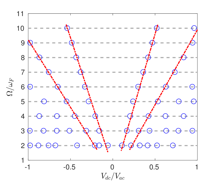
Figure 6: Dependence of multistability regimes on the driving voltage and frequency. The blue circles indicate the approximate positions of the multistability regimes in the parameter plane of driving voltage and frequency. The positions are those at which discontinuous bifurcations occur with respect to the driving frequency for the specific initial condition $\bm{n}(t=0)=(1,0,0)$. The width of each regime depends on the condition. The red dashed lines are included for eye guidance. For relatively small values of $\Omega/\omega_{F}$ (e.g., $2.0$), there are more multistability regimes than those for higher values of $\Omega/\omega_{F}$. The results indicate that the emergence and evolution of multistability can be controlled by the driving frequency.

Multistability in the coupled TI-ferromagnet system can be controlled through parameter perturbations. There are two approaches to altering the final magnetization state. We first fix a particular value of the driving voltage and choose the initial conditions that lead to one of the two possible final states. Transition to the alternative final state can be triggered by applying a perturbation, such as a voltage pulse. Figure 6 shows the approximate locations of the various multistability regimes along the $V_{dc}/V_{ac}$ axis for different values of the driving frequency. For example, for $\Omega/\omega_{F}=7.0$, there are four multistability regimes located approximately at the four points on the line $\Omega/\omega_{F}=7.0$. We then examine the bifurcations for different values of the driving frequency and mark the corresponding transition points in Fig. 6. Since the transition points depend on the initial condition used in calculating the bifurcations, the results are only an approximate indicator of the multistability regimes of finite width. In spite of the uncertainties, we obtain a linear behavior of the multistability regimes in the parameter plane of the driving frequency and voltage. We note that there are irregularities associated with the case of $\Omega/\omega_{F}=2.0$. This is because, in this case, the multistability regimes are too close to each other, rendering indistinguishable to certain extent the transition regimes.

The dependence of the multistability regimes on the driving frequency suggests ease to control the final state. For example, if multistability is undesired, we can choose a relatively high value of the driving frequency, e.g., $\Omega/\omega_{F}=10.0$. In this case, the multistability regimes occupy only a small part of the $V_{dc}/V_{ac}$ interval. That is, for most parameter values there is only a single final state in the system, regardless of the initial conditions. A proper dc voltage can then be chosen to guarantee that the system approaches the desired final state. If the task is to optimize the flexibility for the system to switch between distinct final states, we can set a relatively low value of the frequency, e.g., $\Omega/\omega_{F}=2.0$. In this case, the system exhibits a large number of multistability regimes. Switching between the final states can be readily achieved by using a voltage pulse.

V Discussion

Multistability is a ubiquitous phenomenon in nonlinear dynamical systems GMOY:1983 ; MGOY:1985 ; FGHY:1996 ; FG:1997 ; KFG:1999 ; KF:2002 ; KF:2003a ; KF:2003b ; FG:2003 ; NFS:2011 ; Pateletal:2014 ; PF:2014 , and also in physical systems such as driven nanowire CHLGD:2010 ; NYLDG:2013 and semiconductor superlattice YHL:2016 . Indeed, it is common for a nonlinear system to exhibit multiple coexisting attractors, each with its own basin of attraction GMOY:1983 ; MGOY:1985 . The boundaries among the distinct basins can be fractal GMOY:1983 ; MGOY:1985 or even riddled AYYK:1992 ; OAKSY:1994 ; ABS:1994 ; HCP:1994 ; LGYV:1996 ; LG:1996 ; ABS:1996 ; LA:2001 ; Lai:1997 ; BCP:1997 ; LG:1999b ; Lai:2000 , and there is transient chaos LT:book on the basin boundaries. In applications of nonlinear dynamics, it is thus natural to anticipate multistability. In a specific physical system, to understand the origin of multistability can be beneficial to its prediction and control. Alternatively, it may be possible to exploit multistability for technological systems, such as the development of memory devices.

The purposes of this mini-review article are twofold. First, we introduce topologically protected phases of matter, a frontier field in condensed matter physics and materials science, to the nonlinear dynamics community. For this purpose we provide an elementary description of a number of basic concepts such as Berry phase and Chern number in the context of the celebrated QHE with an emphasis on the topological nature, and topological insulators with dissipationless, spin-momentum locking surface states that are a remarkable source of the spin-transfer torque for nonlinear dynamical magnetization. As a concrete example of a hybrid topological quantum/classical system, we discuss the configuration of coupled TI and ferromagnet, where the former is a relativistic quantum system and the latter is classical. The physical interactions between the two types of systems are discussed: the spin polarized electron flows on the surface of the TI delivers a spin-transfer torque to the magnetization of the ferromagnet, while the latter modifies the Dirac Hamiltonian of the former through an exchange coupling. The nonlinear dynamics of this hybrid system has been studied previously WXL:2016 , including a brief account of multistability. The second purpose is then to present results pertinent to multistability, which were not reported in previous works. Through a detailed parameter space mapping of the regions of multistability, we uncover the phenomenon of alternating multistability, in which the final states of the system emerge and disappear alternatively as some parameters are continuously changed. For example, by changing the frequency of the driving voltage, one can tune the percentage of the multistability regimes in the parameter space. The phenomenon provides a mechanism to harness multistability through experimentally realizable means, such as the delivery of small voltage pulses to the TI.

The system of coupled TI-ferromagnet is a promising prototype of the building blocks for the next generation of universal memory device. The multistable states can potentially be exploited for binary state operation to store and process information.

- (1) H. Sutter, The free lunch is over: A fundamental turn toward concurrency in software. Dr. Dobb J. 30, 202–210 (2005).
- (2) T. Chouard, L. Venema, Machine intelligence. Nature 521, 435–435 (2015).
- (3) Y. LeCun, Y. Bengio, G. Hinton, Deep learning. Nature 521, 436–444 (2015).
- (4) M. I. Jordan, T. M. Mitchell, Machine learning: Trends, perspectives, and prospects. Science 349, 255–260 (2015).
- (5) P. W. Anderson, More is different. Science 177, 393–396 (1972).
- (6) K. Uchida, M. Saitoh, S. Kobayashi, Electron Devices Meeting, 2008. IEDM 2008. IEEE International (IEEE, 2008), pp. 1–4.
- (7) M. Hosomi, et al., Electron Devices Meeting, 2005. IEDM Technical Digest. IEEE International (IEEE, 2005), pp. 459–462.
- (8) R. Takemura, et al., A 32-mb spram with 2t1r memory cell, localized bi-directional write driver and1’/0’dual-array equalized reference scheme. IEEE J. Solid-State Circ. 45, 869–879 (2010).
- (9) B. A. Bernevig, T. L. Hughes, S.-C. Zhang, Quantum spin Hall effect and topological phase transition in hgte quantum wells. Science 314, 1757–1761 (2006).
- (10) M. Z. Hasan, C. L. Kane, Colloquium. Rev. Mod. Phys. 82, 3045–3067 (2010).
- (11) X.-L. Qi, S.-C. Zhang, Topological insulators and superconductors. Rev. Mod. Phys. 83, 1057–1110 (2011).
- (12) P. Gambardella, I. M. Miron, Current-induced spin–orbit torques. Phil. Trans. R. Soc. A 369, 3175-3197 (2011).
- (13) I. M. Miron, et al., Current-driven spin torque induced by the rashba effect in a ferromagnetic metal layer. Nat. Mater. 9, 230–234 (2010).
- (14) I. M. Miron, et al., Perpendicular switching of a single ferromagnetic layer induced by in-plane current injection. Nature 476, 189–193 (2011).
- (15) U. H. Pi, et al., Tilting of the spin orientation induced by rashba effect in ferromagnetic metal layer. Appl. Phys. Lett. 97, 162507 (2010).
- (16) X. Wang, A. Manchon, Diffusive spin dynamics in ferromagnetic thin films with a rashba interaction. Phys. Rev. Lett. 108, 117201 (2012).
- (17) P.-H. Chang, T. Markussen, S. Smidstrup, K. Stokbro, B. K. Nikolić, Nonequilibrium spin texture within a thin layer below the surface of current-carrying topological insulator : A first-principles quantum transport study. Phys. Rev. B 92, 201406 (2015).
- (18) X. Duan, X.-L. Li, Y. G. Semenov, K. W. Kim, Nonlinear magnetic dynamics in a nanomagnet˘topological insulator heterostructure. Phys. Rev. B 92, 115429 (2015).
- (19) K. Taguchi, K. Shintani, Y. Tanaka, Spin-charge transport driven by magnetization dynamics on the disordered surface of doped topological insulators. Phys. Rev. B 92, 035425 (2015).
- (20) M. Jamali, et al., Giant spin pumping and inverse spin Hall effect in the presence of surface and bulk spin- orbit coupling of topological insulator Bi2Se3. Nano Lett. 15, 7126–7132 (2015).
- (21) S. Rex, F. S. Nogueira, A. Sudbø, Topological staggered field electric effect with bipartite magnets. Phys. Rev. B 95, 155430 (2017).
- (22) X.-L. Li, X. Duan, Y. G. Semenov, K. W. Kim, Electrical switching of antiferromagnets via strongly spin-orbit coupled materials. J. Appl. Phys. 121, 023907 (2017).
- (23) J. C. Slonczewski, Current-driven excitation of magnetic multilayers. J. Magnetism Magne. Mater. 159, L1–L7 (1996).
- (24) A. Mellnik, et al., Spin-transfer torque generated by a topological insulator. Nature 511, 449–451 (2014).
- (25) D. C. Ralph, M. D. Stiles, Spin transfer torques. J. Magnetism Mag. Mater. 320, 1190-1126 (2008).
- (26) G.-L. Wang, H.-Y. Xu, Y.-C. Lai, Nonlinear dynamics induced anomalous Hall effect in topological insulators. Sci. Rep. 6, 19803 (2016).
- (27) E. Ott, Chaos in Dynamical Systems (Cambridge University Press, Cambridge, UK, 2002), second edn.
- (28) L. Fu, C. L. Kane, Topological insulators with inversion symmetry. Phys. Rev. B 76, 045302 (2007).
- (29) H. Zhang, et al., Topological insulators in Bi2Se3, Bi2Te3 and Sb2Te3 with a single Dirac cone on the surface. Nat. Phys. 5, 438–442 (2009).
- (30) M. König, et al., Quantum spin Hall insulator state in hgte quantum wells. Science 318, 766–770 (2007).
- (31) D. Hsieh, et al., A topological Dirac insulator in a quantum spin Hall phase. Nature 452, 970–974 (2008).
- (32) Y. Xia, et al., Observation of a large-gap topological-insulator class with a single Dirac cone on the surface. Nat. Phys. 5, 398–402 (2009).
- (33) J. E. Moore, The birth of topological insulators. Nature 464, 194–198 (2010).
- (34) D. J. Thouless, M. Kohmoto, M. P. Nightingale, M. den Nijs, Quantized Hall conductance in a two-dimensional periodic potential. Phys. Rev. Lett. 49, 405–408 (1982).
- (35) F. D. M. Haldane, Model for a quantum Hall effect without landau levels: Condensed-matter realization of the ”parity anomaly”. Phys. Rev. Lett. 61, 2015–2018 (1988).
- (36) M. Schirber, Nobel prize - topological phases of matter. Physics 9, 116 (2016).
- (37) K. v. Klitzing, G. Dorda, M. Pepper, New method for high-accuracy determination of the fine-structure constant based on quantized Hall resistance. Phys. Rev. Lett. 45, 494–497 (1980).
- (38) D. Pesin, A. H. MacDonald, Spintronics and pseudospintronics in graphene and topological insulators. Nat. Mater. 11, 409–416 (2012).
- (39) E. H. Hall, On a new action of the magnet on electric currents. Ame. J. Math. 2, 287–292 (1879).
- (40) R. B. Laughlin, Quantized Hall conductivity in two dimensions. Phys. Rev. B 23, 5632–5633 (1981).
- (41) D. C. Tsui, H. L. Stormer, A. C. Gossard, Two-dimensional magnetotransport in the extreme quantum limit. Phys. Rev. Lett. 48, 1559–1562 (1982).
- (42) R. B. Laughlin, Anomalous quantum Hall effect: An incompressible quantum fluid with fractionally charged excitations. Phys. Rev. Lett. 50, 1395–1398 (1983).
- (43) The Nobel Prize in Physics 1998.
- (44) H. L. Stormer, D. C. Tsui, A. C. Gossard, The fractional quantum Hall effect. Rev. Mod. Phys. 71, S298–S305 (1999).
- (45) J. E. Hirsch, Spin Hall effect. Phys. Rev. Lett. 83, 1834–1837 (1999).
- (46) S. Murakami, N. Nagaosa, S.-C. Zhang, Dissipationless quantum spin current at room temperature. Science 301, 1348–1351 (2003).
- (47) J. Sinova, et al., Universal intrinsic spin Hall effect. Phys. Rev. Lett. 92, 126603 (2004).
- (48) B. A. Bernevig, S.-C. Zhang, Quantum spin Hall effect. Phys. Rev. Lett. 96, 106802 (2006).
- (49) S. Datta, Electronic Transport in Mesoscopic Systems (Cambridge University Press, Cambridge, England, 1995).
- (50) M. König, et al., The quantum spin Hall effect: theory and experiment. J. Phys. Soc. Japan 77, 031007 (2008).
- (51) N. Locatelli, V. Cros, J. Grollier, Spin-torque building blocks. Nat. Mater. 13, 11–20 (2014).
- (52) M. Gajek, et al., Spin torque switching of 20 nm magnetic tunnel junctions with perpendicular anisotropy. Appl. Phys. Lett. 100, 132408 (2012).
- (53) A. Brataas, A. D. Kent, H. Ohno, Current-induced torques in magnetic materials. Nat. Mater. 11, 372–381 (2012).
- (54) M. N. Baibich, et al., Giant magnetoresistance of (001)fe/(001)cr magnetic superlattices. Phys. Rev. Lett. 61, 2472–2475 (1988).
- (55) G. Binasch, P. Grünberg, F. Saurenbach, W. Zinn, Enhanced magnetoresistance in layered magnetic structures with antiferromagnetic interlayer exchange. Phys. Rev. B 39, 4828–4830 (1989).
- (56) The Nobel Prize in Physics 2007.
- (57) I. M. Miron, et al., Perpendicular switching of a single ferromagnetic layer induced by in-plane current injection. Nature 476, 189–193 (2011).
- (58) L. Liu, et al., Spin-torque switching with the giant spin Hall effect of tantalum. Science 336, 555–558 (2012).
- (59) C. Safeer, et al., Spin–orbit torque magnetization switching controlled by geometry. Nat. Nanotech. 11, 143–146 (2016).
- (60) T. Yokoyama, Current-induced magnetization reversal on the surface of a topological insulator. Phys. Rev. B 84, 113407 (2011).
- (61) Y. G. Semenov, X. Duan, K. W. Kim, Voltage-driven magnetic bifurcations in nanomagnet–topological insulator heterostructures. Phys. Rev. B 89, 201405 (2014).
- (62) C. Grebogi, S. W. McDonald, E. Ott, J. A. Yorke, Final state sensitivity: an obstruction to predictability. Phys. Lett. A 99, 415-418 (1983).
- (63) S. W. McDonald, C. Grebogi, E. Ott, J. A. Yorke, Fractal basin boundaries. Physica D 17, 125-153 (1985).
- (64) U. Feudel, C. Grebogi, B. R. Hunt, J. A. Yorke, Map with more than 100 coexisting low-period periodic attractors. Phys. Rev. E 54, 71–81 (1996).
- (65) U. Feudel, C. Grebogi, Multistability and the control of complexity. Chaos 7, 597-604 (1997).
- (66) S. Kraut, U. Feudel, C. Grebogi, Preference of attractors in noisy multistable systems. Phys. Rev. E 59, 5253–5260 (1999).
- (67) S. Kraut, U. Feudel, Multistability, noise, and attractor hopping: The crucial role of chaotic saddles. Phys. Rev. E 66, 015207 (2002).
- (68) S. Kraut, U. Feudel, Enhancement of noise-induced escape through the existence of a chaotic saddle. Phys. Rev. E 67, 015204(R) (2003).
- (69) S. Kraut, U. Feudel, Noise-induced escape through a chaotic saddle: Lowering of the activation energy. Physica D 181, 222-234 (2003).
- (70) U. Feudel, C. Grebogi, Why are chaotic attractors rare in multistable systems? Phys. Rev. Lett. 91, 134102 (2003).
- (71) C. N. Ngonghala, U. Feudel, K. Showalter, Extreme multistability in a chemical model system. Phys. Rev. E 83, 056206 (2011).
- (72) M. S. Patel, et al., Experimental observation of extreme multistability in an electronic system of two coupled Rössler oscillators. Phys. Rev. E 89, 022918 (2014).
- (73) A. N. Pisarchik, U. Feudel, Control of multistability. Phys. Rep. 540, 167-218 (2014).
- (74) Q. Chen, L. Huang, Y.-C. Lai, C. Grebogi, D. Dietz, Extensively chaotic motion in electrostatically driven nanowires and applications. Nano lett. 10, 406–413 (2010).
- (75) X. Ni, L. Ying, Y.-C. Lai, Y. Do, C. Grebogi, Complex dynamics in nanosystems. Phys. Rev. E 87, 052911 (2013).
- (76) L. Ying, D. Huang, Y.-C. Lai, Multistability, chaos, and random signal generation in semiconductor superlattices. Phys. Rev. E 93, 062204 (2016).
- (77) J. C. Alexander, J. A. Yorke, Z. You, I. Kan, Riddled basins. Int. J. Bifur. Chaos Appl. Sci. Eng. 2, 795-813 (1992).
- (78) E. Ott, J. C. Alexander, I. Kan, J. C. Sommerer, J. A. Yorke, The transition to chaotic attractors with riddled basins. Physica D 76, 384-410 (1994).
- (79) P. Ashwin, J. Buescu, I. Stewart, Bubbling of attractors and synchronisation of oscillators. Phys. Lett. A 193, 126-139 (1994).
- (80) J. F. Heagy, T. L. Carroll, L. M. Pecora, Experimental and numerical evidence for riddled basins in coupled chaotic systems. Phys. Rev. Lett. 73, 3528-3531 (1994).
- (81) Y.-C. Lai, C. Grebogi, J. A. Yorke, S. Venkataramani, Riddling bifurcation in chaotic dynamical systems. Phys. Rev. Lett. 77, 55-58 (1996).
- (82) Y.-C. Lai, C. Grebogi, Noise-induced riddling in chaotic dynamical systems. Phys. Rev. Lett. 77, 5047-5050 (1996).
- (83) P. Ashwin, J. Buescu, I. Stewart, From attractor to chaotic saddle: a tale of transverse instability. Nonlinearity 9, 703-737 (1996).
- (84) Y.-C. Lai, V. Andrade, Catastrophic bifurcation from riddled to fractal basins. Phys. Rev. E 64, 056228 (2001).
- (85) Y.-C. Lai, Scaling laws for noise-induced temporal riddling in chaotic systems. Phys. Rev. E 56, 3897-3908 (1997).
- (86) L. Billings, J. H. Curry, E. Phipps, Lyapunov exponents, singularities, and a riddling bifurcation. Phys. Rev. Lett. 79, 1018-1021 (1997).
- (87) Y.-C. Lai, C. Grebogi, Riddling of chaotic sets in periodic windows. Phys. Rev. Lett. 83, 2926-2929 (1999).
- (88) Y.-C. Lai, Catastrophe of riddling. Phys. Rev. E 62, R4505–R4508 (2000).
- (89) Y.-C. Lai, T. Tél, Transient Chaos - Complex Dynamics on Finite Time Scales (Springer, New York, 2011).