CFTP-17-005
SCIPP-17/10
Multi-Higgs doublet models: physical parametrization, sum rules and unitarity bounds
Abstract
If the scalar sector of the Standard Model is non-minimal, one might expect multiple generations of the hypercharge- scalar doublet analogous to the generational structure of the fermions. In this work, we examine the structure of a Higgs sector consisting of Higgs doublets (where ). It is particularly convenient to work in the so-called charged Higgs basis, in which the neutral Higgs vacuum expectation value resides entirely in the first Higgs doublet, and the charged components of remaining Higgs doublets are mass-eigenstate fields. We elucidate the interactions of the gauge bosons with the physical Higgs scalars and the Goldstone bosons and show that they are determined by an matrix. This matrix depends on real parameters that are associated with the mixing of the neutral Higgs fields in the charged Higgs basis. Among these parameters, are unphysical (and can be removed by rephasing the physical charged Higgs fields), and the remaining parameters are physical. We also demonstrate a particularly simple form for the cubic interaction and some of the quartic interactions of the Goldstone bosons with the physical Higgs scalars. These results are applied in the derivation of Higgs coupling sum rules and tree-level unitarity bounds that restrict the size of the quartic scalar couplings. In particular, new applications to three Higgs doublet models with an order-4 CP symmetry and with a symmetry, respectively, are presented.
Keywords:
Higgs physics, Beyond Standard Model, Electroweak interaction, CP violation, Discrete Symmetries1 Introduction
The discovery of the Higgs boson at the Large Hadron Collider (LHC) appears to complete the story of the Standard Model (SM) of particle physics Aad:2012tfa ; Chatrchyan:2012xdj . In particular, the subsequent experimental measurements of the properties of the observed scalar with mass 125 GeV are so far consistent with those of the SM Higgs boson Khachatryan:2016vau . The current Higgs data set is still statistically limited, so a more precise statement is that the observed scalar behaves as a SM-like Higgs boson, to within an accuracy of about . Future experimental studies of the Higgs boson at the LHC will continue to search for deviations from SM behavior, as well as evidence for additional scalar states that might comprise an extended Higgs sector.
Nevertheless, there are numerous reasons to suspect that there must exist new physical phenomena beyond the SM. For example, the SM cannot accommodate dark matter darkmatter , massive neutrinos numass , baryogenesis White:2016nbo and the gravitational interaction. Indeed, there is no fundamental understanding of how the electroweak scale arises, and why this scale is many orders of magnitude smaller than the Planck scale hierarchy . However, the casual observer examining the structure of the SM in its present form might also be puzzled that the set of fundamental scalar fields consists of a single neutral CP-even Higgs boson. After all, the SM employs a direct product of three separate gauge groups and the elementary fermionic matter comes in three generations. Why should one expect a scalar sector to consist only of a single physical state?
In light of the non-minimal structure of the fermionic and gauge bosonic sectors of the SM, one is tempted to suppose that the scalar sector is likewise non-minimal. It is a simple matter to construct an extension of the SM that incorporates an enlarged Higgs sector. In order to preserve the tree-level relation, (which is confirmed by the electroweak data after accounting for electroweak radiative corrections rhoparm ), the electroweak quantum numbers of the Higgs scalar multiplets are constrained HHG ; Ivanov:2017dad . For example, a Higgs sector employing hypercharge- scalar doublets and hypercharge-zero scalar singlets yields , independently of the vacuum expectation values (vevs) of the neutral scalar fields. Following the generational pattern of the fermions, we shall simply replicate the SM Higgs doublet and consider an extended Higgs sector consisting of hypercharge- scalar doublets. For , one must further require that at the minimum of the scalar potential, only the neutral components of the scalar fields acquire vevs NHiggs ; Nishi:2007nh .111The requirement that the electric charge preserving vacuum is a global minimum of the scalar potential imposes some constraints on the scalar potential parameters. Henceforth, we assume that these constraints are respected.
In this paper, we wish to explore various relations among Higgs couplings and bounds on scalar masses that arise in an Higgs doublet extension of the SM. Electroweak gauge invariance plays a central role in determining the structure of the Higgs couplings. Our primary focus here will be the couplings of Higgs bosons to gauge bosons and the cubic and quartic scalar self-couplings. The couplings of the Higgs bosons to fermions is governed by the Yukawa couplings, which must be highly constrained in order to avoid tree-level flavor-changing neutral currents mediated by neutral scalars Glashow:1976nt ; Paschos:1976ay . In this paper, we shall simply postpone the consideration of the scalar-fermion interactions postpone .
Our main tool for obtaining relations among Higgs couplings and constraints on Higgs masses is tree-level unitarity. If one computes the scattering amplitudes for scattering of gauge and Higgs bosons, under the assumption that all Higgs couplings are independent of one another, then one finds that some of the scattering amplitudes grow with the center of mass energy. Such behavior is not consistent with unitarity. Of course, there is no paradox here since the assumption of independent Higgs couplings is incorrect. Electroweak gauge invariance imposes relations among the couplings that guarantee that the bad high energy behavior of any scattering amplitude must exactly cancel. One can turn this argument around and derive relations among the Higgs couplings that are required to cancel the bad high energy behavior of all scattering amplitudes LlewellynSmith:1973yud ; Cornwall:1974km . This procedure allows one to deduce a variety of sum rules that relate various Higgs couplings Weldon:1984wt ; Gunion:1990kf ; Grinstein:2013fia .
Having canceled the bad high energy behavior, one finds that scattering amplitudes in the high energy limit either approach a constant value or vanish in the limit of large center of mass energy. In the former case, the condition of tree-level unitarity imposes an upper limit on the value of this constant. Ultimately, one can show that this constant is a function of dimensionless quartic couplings that appear in the scalar potential. Thus, the imposition of tree-level unitarity yields an upper bound on the values of various combinations of quartic scalar couplings. This in turn can provide upper bounds on some combinations of scalar masses Lee:1977yc ; Lee:1977eg .
In section 2 we consider the most general Higgs doublet model (NHDM). We explicitly write out the couplings of the Higgs bosons to the gauge bosons, which arise from the scalar field kinetic energy terms after replacing the ordinary derivative with the gauge covariant derivatives of the electroweak theory. Remarkably, these couplings are controlled by an matrix , whose physical significance is explained below. We also note the appearance of the matrix . The matrix is an orthogonal antisymmetric matrix that is governed by parameters. These parameters are independent of the basis of scalar fields used to define the model, and thus are related to physical observables.222Given a set of scalar doublet fields , one is always free to consider another basis of scalar fields, that is related to the original set of scalar fields by a unitary transformation. Any physical observable must be independent of the choice of basis. The matrix is governed by physical parameters, which include the parameters that already appear in the matrix . In addition, the matrix depends on (unphysical) phases that can be eliminated by appropriately rephasing the physical charged Higgs fields of the model. We also examine some aspects of the scalar self-couplings. We find that some specific cubic and quartic couplings involving Goldstone boson fields also depend exclusively on the matrices and . This is a consequence of the fact that these interactions terms are related by gauge-fixing to terms appearing in the gauge-covariant scalar kinetic energy terms. The structure of the other cubic and quartic couplings are not as simple, and involve more complicated invariant expressions involving the coefficients of the scalar potential.
In section 3, we derive a variety a sum rules involving the couplings of gauge bosons and Higgs bosons and the couplings of Goldstone bosons and Higgs bosons. In section 4, we present an efficient technique to impose the condition of tree-level unitarity, leading to upper bounds on various combinations of couplings and scalar masses. We apply this to known results and present new results for the three Higgs doublet models (3HDMs) with symmetry and with order-4 CP symmetry, respectively. Conclusions are given in section 5.
In our analysis of the NHDM, one can define a new basis of scalar fields such that the neutral scalar vev resides entirely in one of the Higgs doublet fields, denoted by . This is the well-known Higgs basis Georgi:1978ri ; LS ; BLS ; DH , in which the charged component of is identified as the charged Goldstone boson field and the imaginary part of the neutral component of is the neutral Goldstone boson field. The Higgs basis is not unique, since one is free to make an arbitrary U() transformation among the remaining doublet fields. In particular, one can employ this transformation to diagonalize the physical charged Higgs squared-mass matrix. This procedure yields the charged Higgs basis, as discussed in appendix A. Note that the resulting basis is unique up to an arbitrary separate rephasing of the scalar doublets that contain the physical charged Higgs boson fields.
In appendix B, we apply the analysis of the NHDM given in section 2 to the two-Higgs doublet model (2HDM). We first discuss the complex two-Higgs doublet model (C2HDM), in which a -symmetric scalar potential is softly broken by a complex squared-mass parameter. We then generalize to the most general 2HDM, which is treated using the basis-independent formalism of ref. Haber:2006ue . In both cases, we display the explicit 2HDM forms for the matrices and and exhibit the unphysical parameters in the matrix that can be eliminated by an appropriate rephasing of the physical charged Higgs fields. In appendix C, we demonstrate how to count the number of parameters that govern the matrices and of the NHDM and identify which of these parameters are physical.
In our derivation of coupling sum rules and unitarity relations, the coupling of the Goldstone bosons fields to the physical Higgs fields play an important role. Although the initial forms of these expressions are quite complicated, the corresponding cubic couplings end up reducing to remarkably simple forms. As an example, we provide in appendix D the details of the derivation and simplification of the coupling of two neutral Goldstone fields and a physical Higgs scalar. Finally, in appendix E, we rederive the sum rules obtained directly from the NHDM interaction Lagrangian using an alternative method, which imposes the cancellation of bad high energy behavior in the scattering amplitudes of processes involving the gauge and Higgs bosons. The relation between sum rules involving the neutral Higgs boson couplings to and is clarified in appendix F.
2 Higgs doublet models
In this section we discuss the bosonic Lagrangian of the most general NHDM. The field content consists of the gauge bosons and hypercharge- Higgs doublet fields, parameterized as,
| (1) |
The Higgs-fermion Yukawa interactions will be examined in a subsequent work postpone .
2.1 The scalar potential
For the scalar potential, we follow the notation of BS ; BLS :
| (2) |
where, by hermiticity,
| (3) |
Using eq. (1), the Higgs potential becomes
| (4) |
where,333It is useful to note that, because and are hermitian in , the second term in eq. (7) may be written as
| (5) | |||||
| (6) | |||||
| (7) | |||||
| (8) | |||||
| (9) |
and
| (10) |
is the mass matrix for the charged scalar fields. Requiring the absence of linear terms yields the stationarity condition,
| (11) |
The vacuum of these models has been studied in ref. NHiggs ; here we assume only that the electromagnetic remains unbroken.444Some features of the vacuum of Higgs doublet models have also been studied using the bilinear formalism in refs. Nishi:2006tg ; Nishi:2007nh ; Ivanov:2010ww ; Maniatis:2015gma . Expanding the neutral fields in terms of their real and imaginary components, the second and third terms of may be written as
| (12) |
where [cf. footnote 3],
| (13) | |||||
| (14) | |||||
| (15) |
Using eq. (3), we conclude that is hermitian, the matrices and are real and symmetric, and is a general real matrix. Thus, the mass matrix in eq. (12) is real and symmetric, as expected. Our mass matrices agree with those in ref. NHiggs , after noting that their . Our eq. (15) differs by a minus sign in the last term with respect to a similar eq. (A17) of ref. GL1 . However, this sign error is the result of a misprint, in light of the agreement in signs between our results and eqs. (A18)–(A22) of ref. GL1 .
For later use, we note that
| (16) |
arises from eqs. (15) and (3). From eqs. (13)–(16), we find
| (17) | |||||
| (18) |
Eqs. (5)–(9) are written in with respect to a generic basis of the scalar doublet fields. One can define a new set of charged and neutral scalar fields denoted, respectively, by and , via
| (19) | |||||
| (20) |
where is an unitary matrix, and is a complex matrix. It is convenient to define the real matrix,
| (21) |
Note that the transformation given in eq. (20) results in a real orthogonal similarity transformation of the symmetric squared-mass matrix given in eq. (12). That is is a real orthogonal matrix. As a result, we find
| (22) |
where is the identity matrix. Similarly, from , we obtain,
| (23) |
Hence, it follows that,
| (24) |
Note that we have used the convenient notation of refs. GL2 ; GL3 , which in turn was inspired by refs. GL1 ; Grimus:1989pu . In addition,
| (25) |
Finally, one can show that the matrix is antisymmetric. Moreover, using eqs. (23), this matrix satisfies,
| (26) |
Thus, is the only nontrivial piece of and . As we shall see below, it has the crucial role of controlling scalar couplings involving the boson or its corresponding Goldstone boson. Combining the antisymmetry with eq. (26), we conclude that is orthogonal
| (27) |
In particular, all of its entries satisfy
| (28) |
This will be of interest later.
Let us consider matrices such that
| (29) | |||||
| (30) |
where we have defined
| (31) |
With these choices, the unitarity of implies
| (32) |
while eq. (22) implies
| (33) | |||||
| (34) | |||||
| (35) |
where the last equality holds because is antisymmetric in . We wish to study the squared-mass matrix of the charged scalars with respect to the charged scalar fields ,
| (36) |
Using eqs. (10), (29), and (11), it is easy to show that
| (37) |
This means that with respect to the charged scalar fields [reached by transformations with (29)], the first row and first column of the transformed squared-mass matrix of the charged scalars vanishes. This identifies with the charged would-be Goldstone boson ,
| (38) |
Next, we turn to the squared-mass matrix of the neutral scalar fields.
Using eq. (30), we start by looking at
| (45) | |||||
For the first equality, we have used eqs. (13) and (15). To reach the last line of eq. (45), we have used eq. (31) and the stationarity condition given in eq. (11). Similarly,
| (46) | |||||
Multiplying eq. (45) by , multiplying eq. (46) by , and summing over , we conclude from eq. (2.1) that
| (47) |
where the first equality holds since is a real symmetric matrix. This means that with respect to the scalar fields , [reached by transformations with (30)], the first row and first column of the transformed squared-mass matrix of the neutral scalars vanishes. This identifies with the neutral would-be Goldstone boson ,
| (48) |
One can choose matrices and in such a way that the transformations in eqs. (19) and (20) yield the charged and neutral scalar mass eigenstate fields, respectively,
| (49) | |||||
| (55) |
Since we have identified and , it follows from our above analysis that the matrices and must satisfy eqs. (29) and (30), respectively. In this case, and denote the fields of the physical charged and neutral scalar particles, respectively. Their corresponding masses are and .555In appendix A we discuss two other ways to identify the neutral and charged scalar mass eigenstate fields, involving intermediate steps which simplify some of the analysis.
Using eqs. (49)–(55) in eqs. (17)–(18), we end up with
| (56) | |||||
| (57) |
These are the only combinations of quartic couplings (and vevs) that one can obtain from the diagonalization of the scalar squared-mass matrices. Thus, only those cubic and quartic terms of the scalar potential involving these combinations will be related to scalar masses. Eqs. (56)–(57) constitute a crucial result of our paper, since, they will enable us to relate the gauge-Higgs couplings with the scalar-scalar couplings.666This is, of course, consistent with gauge-fixing and is needed, in particular, for the equivalence theorem.
2.2 Gauge-Higgs couplings
When expressed in terms of the physical gauge fields, the gauge covariant derivative may be written as
| (58) |
where is the coupling constant, , , is the electric charge of the positron, is the charge operator, and777In this paper, we normalize the hypercharge such that , where .
| (59) |
when acting on SU(2) doublets. Note that the signs of the coupling constants and gauge fields above correspond to choosing all the equal to in the notation of ref. Romao:2012pq . This coincides with the conventions of ref. HHG , but differs in the signs in from refs. djouadi1 ; djouadi2 .888The signs in refs. BLS ; GL2 correspond to yet another choice, which yields an unexpected sign in the relation . This also has an impact on any Feynman rules proportional to or .
The kinetic term for the scalar fields is
| (60) |
We substitute eq. (58) and parameterize the as in eq. (1). Next, we employ eqs. (19)–(20) to express the charged and neutral fields in terms of the mass eigenstate fields, and we use the properties in eqs. (22)–(35). We end up with,
| (61) | |||||
where,999We employ the notation where .
| (62) | |||||
| (63) | |||||
| (64) | |||||
with and
| (65) | |||||
| (66) |
are matrices of dimension and , respectively.
The matrix is basis-independent and hence physical, whereas the matrix is basis-independent up to unphysical phases that can be absorbed into the definition of the physical charged Higgs fields, (for ). Further details will be provided in the next section. Eqs. (61)–(64) agree with eqs. (29a)–(29p) of ref. GL2 , if we notice that, because of the different sign in the coupling , we have , , and , where the subscript “GLOO” stands for ref. GL2 . The only exception is in the coupling given in eq. (63) which, after the difference in notation is properly accounted for, disagrees with the sign of eq. (29h) of ref. GL2 . We have checked in both notations that their incorrect sign can be attributed to a misprint.
2.3 The and matrices
In section 2.2 we showed that the couplings arising from the kinetic Lagrangian depend exclusively on the matrix in the charged scalar sector and on in the neutral scalar sector. and are defined in terms of the matrices and , which relate the charged and neutral fields in a generic basis of scalar fields, , to the corresponding mass-eigenstate scalar fields, respectively. The choice of basis is of course arbitrary. For example, another set of scalar fields , with
| (67) |
where is some unitary matrix, could have been employed. The scalar field kinetic energy terms are invariant with respect to eq. (67), since
| (68) |
which follows from . Consequently, the interactions of the scalars with the gauge bosons given by eqs. (61)–(64) are basis-independent. Indeed, any physical observable cannot depend on the choice of basis. We would like to use these observations to address the behavior of the matrices and under an arbitrary change of basis. The interaction Lagrangian given by eqs. (61)–(64) is written in terms of the scalar mass eigenstates and , which are related via eqs. (19) and (20) to the scalar fields in a generic basis. The diagonalization of the neutral scalar squared-mass matrix is given by eq. (2.1) and yields real neutral scalar mass-eigenstate fields. The overall sign of the neutral scalar mass-eigenstate fields are not physical. However, the standard practice is to fix this sign by appropriately restricting the range of the angles that parameterize the diagonalization matrix. Having adopted this convention where the sign of the neutral scalar mass-eigenstate fields are fixed, it follows that the matrix that appears in eqs. (62) and (63) is basis-independent and hence physical.
In contrast, the diagonalization of the charged scalar squared mass matrix yields complex mass-eigenstate charged scalar fields. By convention, the phase of the charged Goldstone field is fixed. In particular, it is convenient to choose in eq. (67), which yields the scalar field basis,
| (69) |
where are the physical (mass-eigenstate) charged Higgs fields with corresponding masses . This is called the charged Higgs basis and has two defining properties:
-
1.
, , , , are the charged scalar mass-eigenstate fields;
-
2.
the first doublet field, , has the massless would-be Goldstone boson as its charged (upper) component, and its phase has been chosen such that the (real and positive) vev, GeV, is contained in the real part of its neutral (lower) component.
The Higgs basis (which is defined by property 2 alone) and the charged Higgs basis are discussed in detail in appendix A. Notice that the fields and are not the neutral scalar mass-eigenstate fields. is the matrix that transforms these fields, written in the charged Higgs basis, into the neutral scalar mass-eigenstates.
The charged Higgs basis is unique up to a possible rephasing of the charged Higgs fields, [for ]. That is, the charged Higgs basis is a family of scalar bases that is characterized by phases, , as discussed at the end of appendix A. In eqs. (63) and (64), the invariant combinations and its charged conjugate appear. Hence, it follows that the matrix is not quite basis-independent, since [for ] under the rephasing of the charged Higgs fields to preserve the invariance of eqs. (63) and (64).
In contrast, the mixing matrices and that relate the charged and neutral fields in a generic basis of scalar fields, , to the corresponding mass-eigenstate scalar fields, respectively, are basis dependent. It is instructive to examine the question of basis dependence and work out the explicit forms of the matrices and in the more familiar 2HDM. In this case, the matrix contains the angle . As discussed at length in ref. Haber:2006ue , this means that the angle does not in general have a physical meaning, since the vevs and (and hence ) transform under the basis transformation given by eq. (67). Similarly, the mixing angle parameters appearing in the matrix that transforms the neutral scalar fields of the generic basis into the neutral scalar mass-eigenstate fields are also basis dependent. To find basis-independent quantities, one must consider the neutral mixing angle parameters relative to the angle . That is, under a basis transformation, both the neutral mixing angle parameters and the angle shift by the same amount so that their difference is invariant. Thus, one way to determine the invariant neutral mixing angle parameters is to work in the Higgs basis, in which . Further details can be found in appendix B. The matrix is the NHDM generalization of the neutral mixing angle parameters relative to the angle . As noted above, the matrix is almost basis-invariant, since unphysical phases remain that reflect the possible rephasing of the charged Higgs fields.
From section 2.1, we can deduce the following properties of the matrices and . First, it is convenient to re-express in terms of the matrix defined in eq. (21). We introduce the orthogonal antisymmetric matrix , which in block form is defined by
| (70) |
Then can be rewritten as,
| (71) |
It immediately follows that is a real orthogonal and antisymmetric matrix; i.e.,
| (72) |
In particular, the orthogonality of implies that .
Given an unitary matrix , it is always possible to represent this matrix by the following real orthogonal matrix,
| (73) |
Henceforth, we shall always identify the real orthogonal representation of a unitary matrix with a subscript and a tilde (to indicate that the dimensionality of the matrix has been doubled).
Using this notation, it is convenient to construct the matrix ,
| (74) |
Since and are real orthogonal matrices, it follows that is also a real orthogonal matrix. Moreover,
| (75) |
Noting that and , one can write
| (76) |
Finally, we note that
| (77) |
The central point of this section is the following. Unless there is an (imposed symmetry) reason to single out some specific basis, the best way to count parameters and to set up a numerical simulation is to write the potential in the charged Higgs basis ab initio. As seen from appendix A, the charged Higgs basis is (almost) unique, up to the separate rephasing of the doublets with zero vev. As a result, all the parameters of the scalar potential, when written in the charged Higgs basis, are either invariant or pseudo-invariant quantities with respect to arbitrary scalar basis transformations. Here, pseudo-invariant means invariant up to an overall phase that arises from the rephasing of the doublets that contain the physical charged Higgs fields. It is straightforward to construct invariants from appropriate products of pseudo-invariants in which the overall phase ambiguity cancels. All such observable quantities are potential experimental observables. This provides the generalization of the parameters and championed for the 2HDM in ref. Zs .
2.4 Parameter counting
We begin by asking the following question. How many parameters govern the matrices and and how many of these parameters are physical? To address this question, we first examine the matrices and , which transform the neutral and charged scalar fields of a generic basis to the corresponding scalar-mass eigenstates, respectively.
Starting from a scalar basis, , one can compute the neutral scalar squared-mass matrix as shown in eq. (55). The real orthogonal diagonalizing matrix is related to the matrix defined in eq. (20) via eq. (21). With respect to a new scalar basis , one obtains a new matrix given by
| (78) |
after using eqs. (20) and (67). Employing eqs. (21) and (78), one obtains a new real orthogonal diagonalizing matrix given by
| (79) |
where [following eq. (73)] the real orthogonal matrix is defined by
| (80) |
Using eq. (299), one can decompose the real orthogonal matrix , where and are the real orthogonal matrices given in eq. (300). Inserting this result back into eq. (80) yields,
| (81) |
Using the definition of the matrix given in eq. (66), one can determine with respect to a new scalar basis ,
| (82) |
Note that the same result can be obtained by employing eqs. (71) and (79), since
| (83) |
after noting that (the latter makes use of the fact that is unitary). That is, is basis-independent. In particular, if we choose in eq. (81), then , which can be expressed in terms of parameters.101010Since , we can use the results of appendix C.3 to show that , which depends on two real antisymmetric matrices, is governed by parameters. Consequently, eq. (83) implies that , which depends on physical parameters.111111This result is consistent with eq. (72), since the most general real orthogonal antisymmetric matrix can be expressed in terms of independent parameters, as shown in appendix C.1.
Likewise, starting from a scalar basis, , one can compute the charged scalar squared-mass matrix as shown in eq. (49). The unitary diagonalizing matrix defined in eq. (19) depends on the basis. One also must take into account that the charged Higgs basis is not uniquely defined, as discussed at the end of appendix A. Hence, the physical charged Higgs fields may acquire phases under the basis change. If we perform a basis transformation given by eq. (67), we must allow for the possibility that [for ]. We can write the latter as
| (84) |
where the primes indicate quantities associated with the transformed basis and
| (85) |
Combining eqs. (19), (67) and (84) yields
| (86) |
where
| (87) |
That is, one obtains a new unitary diagonalizing matrix given by
| (88) |
where there is an implicit sum over the repeated index .
We can now compute the transformation of under a change of scalar basis. With respect to the basis , we have
| (89) | |||||
| (90) |
If we consider the charged Higgs basis where , then eq. (87) yields and
| (91) |
after making use of eqs. (74) and (81) with . The phases (for ) that appear (and similarly are contained in ) are unphysical and can be absorbed into the definition of the charged Higgs fields . Since (unless the neutral Higgs fields are mass eigenstates in the charged Higgs basis), it follows that contains additional parameters beyond the physical parameters that determine the matrix . As shown in appendix C.2, the matrix (and ) depends on an additional physical parameters. That is, after absorbing the phases into a redefinition of the charged Higgs fields, there are physical parameters remaining in the matrix (and ).
The C2HDM provides an interesting example, discussed in detail in appendix B. One sees in eq. (260) that (or equivalently ) depends on angles, where one of the angles is unphysical and corresponds to the freedom to rephase the second scalar doublet with zero vev. In contrast, in eq. (267) depends only on the two invariant angles contained in . The case of is special in that the parameters that define the matrix corresponding precisely to the physical parameters that appear in the matrix .
The physical parameters contained in the matrix are sufficient to parameterize all the gauge boson–Higgs boson interactions. But, the three-scalar and four-scalar interactions derived from the scalar potential necessarily involve additional parameters. We have already emphasized that the charged Higgs basis is especially useful in identifying the invariant (and pseudo-invariant) scalar self-coupling coefficients. In particular, in the charged Higgs basis, the scalar potential is given by
| (92) |
The number of relevant parameters is shown in table 1.
| parameters | magnitudes | phases | |
|---|---|---|---|
| and |
The number of parameters gets reduced for two reasons. First, our definition of the charged Higgs basis allows for a rephasing of the scalar doublets with zero vevs. This reduces the number of phases by . In addition, the stationarity conditions written in the charged Higgs basis relate some and parameters. More generally, eq. (197) can be used to obtain a relation of the and parameters with the charged scalar masses,
| (93) |
which can be used to trade in the for the parameters and the charged scalar masses. Hence, using the charged Higgs basis as parameters, we need only the magnitudes and the phases in , of which only phases are physical.
For example, in the 2HDM and in the notation of ref. Zs , we find
| (94) |
The seven magnitudes correspond to and the two independent phases are and , first identified in ref. LS as basis invariant measures of CP violation. Although not independent in the case , the possibility of is only covered by considering in addition the third invariant phase, LS ; DH .
Many different parameter choices exist in the literature. For example, one can employ: (i) and the quartic coefficients of the scalar potential in the charged Higgs basis; or (ii) the quadratic coefficients not fixed by the scalar potential minimum conditions and all of the quartic coefficients ; or (iii) the physical parameters in , the physical charged and neutral scalar masses, and (if needed) some invariant combination of scalar self-couplings. In extended Higgs sectors with additional symmetries (where the basis in which the symmetries are manifest becomes physical), one can also employ the various ratios of scalar vevs in the list of parameters. For example, in the CP-conserving 2HDM with a softly-broken -symmetric scalar potential, some authors choose parameters consisting of , [which appears in the matrix in our notation], the charged scalar mass , the neutral scalar masses (, , and ), and the soft breaking squared-mass term .
2.5 Scalar self-couplings
In this section, we demonstrate that some of the scalar self-couplings are related to the kinetic terms obtained in section 2.2. In particular, it is convenient to enquire which scalar couplings may be written exclusively in terms of the matrix (and ), that appear in the kinetic terms, and the scalar masses and .
We first consider the cubic scalar self-couplings. The scalar potential in eqs. (4)–(9) can be expressed in terms of the physical fields using the mixing matrices and in eqs. (19)–(20). The cubic vertex interactions can therefore be written as
| (95) | |||||
In contrast to the terms of the interaction Lagrangian that couple the scalar and vector bosons given in eqs. (61)–(64), additional structures appear beyond those combinations of and that define the matrices and . However, if we focus on the cubic couplings that involve at least one Goldstone field, the form of the cubic interaction terms simplify significantly and can be expressed in terms of the and matrices and the squared masses of the physical scalars.121212In particular, we find that the couplings , , , and vanish. The vanishing of the , and couplings is a well-known result of the SM. Indeed, this is to be expected, as these interaction terms are related by gauge-fixing to the pure gauge boson terms arising from the kinetic Lagrangian, which can be expressed in terms of the matrices and , as shown in eqs. (61)–(64).
In order to simplify the non-vanishing cubic potential terms we employ eqs. (22)–(35), from which we obtain the further useful relations
| (96) | |||||
| (97) | |||||
and
| (98) | |||||
| (99) |
Moreover, we must use the crucial relations given in eqs. (56)–(57), relating some combinations of quartic couplings with the scalar masses. This simplifies considerably the final expressions. The end result is,131313The expressions for the cubic couplings of the Goldstone bosons and physical Higgs scalars in terms of scalar squared-masses was first obtained in the CP-conserving 2HDM in Ref. Gunion:2002zf .
-
•
For :
(100) -
•
For :
(101) -
•
For :
(102) -
•
For :
(103)
where there is an implicit sum over repeated indices. Achieving the simplified forms of the couplings above is rather laborious. For example, the explicit derivation of eq. (103) is given in appendix D.
The cubic couplings that are present in the kinetic lagrangian are also present in parallel with the scalar potential. A comparison is shown in table 2, where we have collected the relevant Feynman rules.
| Kinetic lagrangian | Scalar potential | ||
|---|---|---|---|
| Coupling | Feynman rule | Coupling | Feynman rule |
| Null | |||
| , | Null , | ||
| , | , | ||
| , | , | ||
| , | , | ||
| , | , | ||
| Null | |||
| , | , | ||
| , | , | ||
We notice that both sets of couplings depend on the same parameters:
| (104) |
This is not surprising, since gauge boson couplings and Goldstone boson couplings are related by the gauge-fixing, as previously noted. Although the equivalence theorem Veltman:1989ud is not a requirement on the couplings but rather on full processes miguel , the relation between these couplings insures that the equivalence theorem is satisfied.
For the calculation of the quartic couplings we use the general expression
| (105) | |||||
It is instructive to focus on the quartic couplings that involve the Goldstone boson fields. After some very long simplifications, we find the non-vanishing Goldstone-scalar quartic couplings that involve an even number of Goldstone boson fields listed below.
-
•
For :
(106) -
•
For :
(107) -
•
For + h.c.:
(108) -
•
For :
(109) -
•
For :
(110) -
•
For :
(111) -
•
For :
(112) -
•
For :
(113) -
•
For + h.c.:
(114)
The corresponding expressions involving an odd number of Goldstone fields are more complicated and will not be given here.
In contrast to the cubic couplings given in eqs. (100)–(103), additional structures beyond the matrices , and the squared masses of the physical scalars appear in the expressions above. For example, the quadratic coefficient of the scalar potential in the charged Higgs basis, , appears on the right hand side of eq. (107). Note that there is no simple relation between quartic couplings in the kinetic Lagrangian and quartic terms from the scalar potential. For example, as in the SM, there is a coupling, but no coupling. This does not violate the equivalence theorem since the processes involving quartic couplings typically involve other diagrams. In particular, only the sum of all contributing diagrams must obey the equivalence principle.
3 Sum rules
3.1 Coupling relations and sum rules from the Lagrangian
One can obtain a large number of sum rules from the kinetic part of the Lagrangian and the scalar potential of the NHDM. In the case of the 2HDM, two of the sum rules that are usually exhibited (see, e.g., refs. Gunion:1990kf ; Grinstein:2013fia ; abdss ; Arhrib:2015gra ) are
| (115) |
where identifies some specific neutral scalar physical field. It is easy to find the corresponding sum rules in the general NHDM:
| (116) | |||||
| (117) |
where the indices follow the same notation as above. In this section we use a simplified notation for the couplings, strictly related to the matrices and , in which some coupling is identified as the term in the Lagrangian that depends explicitly on family type indices. For example, in the Lagrangian term
| (118) |
involving the fields , , and the constant , we identify . In cases where the corresponding coupling also exists in the SM, this procedure means simply that we have divided out by the SM coupling .
In addition to these, we have found many sum rules for an arbitrarily extended scalar doublet sector. For example,
| (119) |
Using this result in eq. (117), and recalling that , we find
| (120) | |||||
| (121) |
Further equations arising from the kinetic Lagrangian are
| (122) | |||||
| (123) | |||||
| (124) |
The relations among different couplings in the kinetic Lagrangian imply that one can write eq. (123) in terms of massive fields (i.e., without the Goldstone bosons) as
| (125) |
We have checked that all our relations are verified when using the couplings in the special case of the C2HDM. Notice that eqs. (119) and (122) are not proper sum rules, but rather relations among couplings valid in our particular model.
These sum rules have been found by employing the NHDM interaction Lagrangian. But we know that sum rules can also be found for generic Lagrangians by using unitarity arguments, as in refs. Gunion:1990kf ; Grinstein:2013fia . The sum rules we have derived in eqs. (116) and (120)–(122) can also be found in that fashion. We will revisit this question in section 3.2 and in appendix E.
In the quartic couplings sector, we have found further interesting sum rules. For example, using the couplings in eq. (107), we find141414Note that is a basis-invariant quantity.
| (126) |
which has the peculiar feature that a sum of couplings involving solely charged particles yields a contribution that depends on the masses of the neutral fields. Similarly, using the couplings in eq. (112), we find
| (127) |
We can recombine a number of these sum rules as
| (128) |
or
| (129) |
because the following equation is satisfied,
| (130) |
The sum rules involving quartic couplings presented in eqs. (126)–(130) are new.
3.2 Sum rules from unitarity
The constraints from unitarity have had an historical impact on the development of particle physics. The idea is that the scattering among vector bosons and/or scalars cannot grow with energy and must obey the optical theorem. Imagine that one writes the most general effective couplings between these states, up to dimension four. Forcing the sum of all terms growing like the fourth power of the center of mass energy () to vanish immediately restricts the vector bosons to originate from a gauge theory Cornwall:1974km ; LlewellynSmith:1973yud . Requiring that all terms vanish forces the scalar-gauge couplings to originate from a gauge theory and further constrains the couplings Weldon:1984wt ; Gunion:1990kf . But unitarity also limits the value of the constant in the terms. This has been used in the past to place limits on (combinations) of the scalar masses and couplings Lee:1977yc ; Lee:1977eg ; Weldon:1984wt ; Grinstein:2013fia .
In the previous section we derived the coupling relations (119) and (122) and many sum rules directly from the Lagrangian of the NHDM. We have checked that most sum rules involving triple couplings can be obtained from those presented in ref. Gunion:1990kf , by applying them to the NHDM and cycling through all possible indices. The exception arises in applying eqs. (116) and (117) for the case of , which are presented in ref. Gunion:1990kf under the assumption of CP conservation. For completeness, we include in appendix E a careful and detailed derivation of the sum rules given in eqs. (2.4)–(2.6) of ref. Gunion:1990kf . The derivation of these sum rules does not make use of CP conservation. Nevertheless, when applied to models with scalars in their section IV, the authors of ref. Gunion:1990kf focus on models that conserve CP. In particular, they point out that requiring CP conservation, , and leads, through their eq. (4.5), to , thus turning sum rules that involve into sum rules involving in the case of a CP conserving Higgs sector. In contrast, the general NHDM may (or not) violate CP; nevertheless, the same sum rules apply. We include in appendix F a proof that , which makes no assumption concerning CP conservation, and yet is valid for scalars in any representation of , provided that the theory satisfies without fine tuning of the various vevs.
4 Tree-level unitarity bounds
In this section, we present an algorithm for the determination of the tree-level unitarity bounds. We check that it reproduces results available in the literature, and present its application to two new cases with three Higgs doublets. Finally, the techniques presented here can be used for faster numerical implementation of unitarity bounds in more complicated cases, not amenable to closed-form solutions.
The problem of finding the constraints imposed by tree-level unitarity has been addressed in the case of the 2HDM, both with symmetry Ginzburg:2003fe and also for most general case Ginzburg:2005dt ; Kanemura:2015ska . For the 2HDM with a symmetric scalar potential, the results are simple, but for the most general case one has to compute the eigenvalues of and matrices Ginzburg:2005dt ; Kanemura:2015ska . For the case of the 3HDM a solution is known for the case of symmetry Das:2014fea where because of the symmetry the solutions are again simple, although the method to obtain them is already quite complicated.
Clearly, for the NHDM one needs an algorithm that can be easily implemented numerically. As explained in the references above, since one is interested in the high energy limit, one just needs to evaluate the scattering -matrix for the two body scalar bosons, and these arise exclusively from the quartic part of the potential, . Then, the first part of the problem consists in finding the set of two body states that can contribute. For the cases of low and high symmetry we can choose conveniently the sets to take advantage of this Ginzburg:2003fe ; Ginzburg:2005dt , but if we are going to solve the problem numerically it is better to have a simple algorithm of general applicability. Since the electric charge and the hypercharge are conserved in this high energy scattering, we can separate the states according to these quantum numbers. For this it is better not to separate the real and imaginary parts of the neutral components, using the following notation for Higgs doublets
| (131) |
The relevant two body states are given in the entries of table 3, and their complex conjugates.
| State | Number of states | ||
|---|---|---|---|
| 2 | 2 | , () | |
| 1 | 2 | , () | |
| 1 | 0 | , () | |
| 0 | 2 | , () | |
| 0 | 0 | , () |
As an example, for we have,
| (132) | ||||
| (133) | ||||
| (134) | ||||
| (135) | ||||
| (136) |
plus their complex conjugates. It is important to note that the index is a compound index; it refers to a set of indices. Also note that in eqs. (132) and (135) the two body states with equal particles have a normalization of that we have not written here (see below).
Now we separate the different partial wave amplitudes for the different charges and hypercharges. We have
| (137) | |||||
| (138) | |||||
| (139) | |||||
| (140) | |||||
| (141) |
where we have indicated on the right-hand side the dimensionality of the resulting matrices. The compound nature of the index should be taken in account. For instance
| (142) |
where the set corresponds to and the normalization is for the 2 body states with equal particles and 1 in all the other cases. This factor can be understood in the following way. When we take the derivative with respect to the 2 body state with equal particles we should divide by the normalization . But on the right-hand side we are taking derivatives with respect to the individual fields. To avoid double counting we should divide by two in the case of identical particles, so .
This procedure can be easily implemented in an algebraic program like Mathematica and we can easily obtain the five matrices . For simple cases we can obtain the eigenvalues; for the more complicated cases we can obtain the characteristic equation and solve it numerically for the eigenvalues.
For illustration, consider the case of the 2HDM. The quartic part of the potential contains
| (143) |
Using the procedure described above one can easily get for ,
| (144) |
which coincides with the result of ref. Kanemura:2015ska , up to an interchange of rows and columns.
We have applied this procedure for the known cases in the literature and, to illustrate the power of the method, we also present two new cases.
4.1 An (almost) trivial case: the Standard Model
Consider the Standard Model with . With the conventions of ref. Romao:2012pq , we have
| (145) |
In this case the matrices reduce to
| (146) |
There are therefore two independent eigenvalues,
| (147) |
Applying partial wave unitarity to the eigenvalues of the -wave amplitude matrix, which is a consequence of the optical theorem,
| (148) |
Eq. (148) implies that
| (149) |
Since the right hand side of eq. (149) is bounded by , it follows that Luscher:1988gc ,
| (150) |
which translates into
| (151) |
This in turn implies
| (152) |
a well known result Lee:1977yc ; Lee:1977eg .
4.2 Other known cases
We applied the method to the complex 2HDM with symmetry and we recover the results of ref. Ginzburg:2003fe ; Ginzburg:2005dt . Next we studied the general complex 2HDM and we also agree with the results of ref. Ginzburg:2005dt ; Kanemura:2015ska . Both these cases are for . A more complicated case is the 3HDM with symmetry. The matrices are larger but we were able to recover all the results of ref. Das:2014fea . This makes us confident that the procedure can be generalized to cases where the unitarity constraints have not been studied. We consider two new cases.
4.3 The 3HDM with order-4 CP symmetry
Consider the potential of the 3HDM with order-4 CP symmetry given in ref. Ivanov:2015mwl ,
| (153) |
with all parameters real except for , that are complex. Applying the method we get the following distinct eigenvalues for the matrices,
| (154) | ||||
| (155) | ||||
| (156) | ||||
| (157) | ||||
| (158) | ||||
| (159) | ||||
| Roots of: | ||||
| (160) | ||||
| Roots of: | ||||
| (161) | ||||
| Roots of: | ||||
| (162) |
4.4 The 3HDM with symmetry
As a second example, we consider the potential for the 3HDM with a symmetry Ferreira:2008zy , that we write in the form
| (163) |
where the parameters and are real, while are complex. We get the following eigenvalues of the matrices:
| (164) | ||||
| (165) | ||||
| (166) | ||||
| (167) | ||||
| (168) | ||||
| (169) | ||||
| Roots of: | ||||
| (170) | ||||
| Roots of: | ||||
| (171) | ||||
| Roots of: | ||||
| (172) | ||||
| Roots of: | ||||
| (173) |
4.5 Unitarity bounds for specific processes in the NHDM
In the previous sections, we have presented an algorithm which computes tree-level unitarity bounds on a given chosen model of scalar doublets. The method of Lee, Quigg and Thacker Lee:1977yc ; Lee:1977eg , which we have generalized and optimized, yields necessary and sufficient conditions for tree unitarity in the scalar and gauge sectors of any NHDM. A possible shortcoming of this method is the computational time needed to find all the eigenvalues for each point in parameter space in the case of a general scalar doublet theory, i.e. without symmetries, or with a large .
A complementary approach of finding necessary, although not sufficient conditions for every NHDM can be attained by using unitarity bounds on specific processes. Therefore, we can compute the partial-wave coefficient for gauge-gauge and gauge-scalar scatterings, using that from the optical theorem , and that we can use the Equivalence Theorem to simplify calculations. The Equivalence Theorem allows us to perform all calculations from the scalar potential, and therefore, we can always define
| (174) |
where stands for the amplitude of the process. Another important property of this method, also used in the previous section, is that we will only consider the quartic couplings contribution at high energy. We use this simple approach to work out some examples in the NHDM for an arbitrary .
4.5.1 The process
As a first example, we consider the process with amplitude , which we approximate at high energies to . The leading order contribution for the process will be the quartic coupling with amplitude
| (175) |
where we have used eq. (106) and the notation from section 3. It is straightforward to see that this process enforces the bound
| (176) |
It is interesting to note that in the alignment limit of the coupling we cannot further constrain any masses of new neutral scalars. This observation is due to the bound in the matrix itself, which is orthogonal, implying that . This bound is given as a special case of eq. (2.10c) of ref. Weldon:1984wt , and it is valid in any NHDM.
4.5.2 The process
We now turn to the unitarity bounds arising from the scattering. Using the same reasoning as before, we use the quartic coupling of eq. (113). We then have
| (177) |
where is the quadratic parameter of the lagrangian in the charged Higgs basis. Using the optical theorem we find that
| (178) |
Although one cannot predict mass bounds for the charged scalars in this process, it is possible to study numerically the dependence on a given choice of . This parameter in the charged Higgs basis is a physical one and can, in principle, be measured.
4.5.3 The process
As a final example we compute the unitarity bounds for the process . We follow the same arguments as before and write the quartic coupling in eq. (107) as
| (179) |
where is the coupling to and is the coupling to . We can therefore use the optical theorem to obtain,
| (180) |
It is convenient to rewrite eq. (180) as,
| (181) |
so that the dependence on cubic couplings is explicit.
5 Conclusions
We have studied the most general theory with Higgs doublets. We have stressed the importance of the charged Higgs basis, where the magnitudes and basis-invariant combinations of phases of its scalar couplings and are observables. The kinetic Lagrangian depends exclusively on a matrix , or equivalently the real orthogonal matrix as defined in eq. (74), which governs the relation between the neutral scalar components of the scalar doublets in the charged Higgs basis and the neutral Higgs mass eigenstates. The matrix (or ) depends on unphysical phases (corresponding to the non-uniqueness of the charged Higgs basis) and on physical parameters. Of these, appear in the special combination .
Although new parameters beyond appear in the scalar potential, many couplings involving the Goldstone bosons and can be related to couplings involving and , as expected from consistency with gauge fixing. We use the crucial eqs. (56)-(57) to show that such relations indeed hold. This is also consistent with bounds from unitarity, which are discussed in great detail. In particular, we develop an efficient algorithm for the inclusion of such bounds in NHDM and employ it in two new 3HDM models with a and with a order-4 CP symmetry, respectively. Some model independent necessary constraints are shown, by applying the optical theorem to selected processes.
In models where the scalar potential exhibits additional symmetries, some new parameters may appear to arise, relating the original basis to the charged Higgs basis (thereby acquiring physical significance). For example, such a case arises in the the 2HDM with a -symmetric scalar potential, where is the angle that rotates the basis in which the symmetry is manifest into the charged Higgs basis. But, such parameters can always be re-expressed in terms of those discussed here [e.g., as shown for in eqs. (51) and (52) of ref. Zs ]. New parameters do arise when fermions are included, which will be addressed elsewhere postpone .
Acknowledgements.
We are very grateful to A. Barroso for collaboration in the initial stages of this work and to M.J. Gouveia for discussions on matrices. J.P.S. is grateful to “Taberna do Avillez”, where part of this work was made. The work of M.P.B, J.C.R. and J.P.S. is supported in part by the Portuguese Fundação para a Ciência e Tecnologia (FCT) under contracts CERN/FIS-NUC/0010/2015 and UID/FIS/00777/2013. H.E.H. is supported in part by the U.S. Department of Energy grant number DE-SC0010107. H.E.H. acknowledges the hospitality and the inspiring working atmosphere of the Aspen Center for Physics, supported by the National Science Foundation Grant No. PHY-1066293, where some of the research reported in this work was carried out.Appendices
Appendix A The Higgs basis and the charged Higgs basis
In section 2.1, we have discussed how to determine the physical charged and neutral scalar mass eigenstates starting from a generic basis of scalar fields . The charged and neutral components of the th scalar doublet can be expressed as linear combinations of the physical charged and neutral scalar mass eigenstates [cf. eqs. (19) and (20), respectively], where the corresponding coefficients define the matrices and . To find the physical couplings, we first determine the scalar potential minimum conditions in the original (generic) basis (these stationarity conditions given in eq. (11) are complicated coupled cubic equations in the vevs, ). Substituting these conditions back into eqs. (7)–(9) and re-expressing the generic basis scalar fields in terms of the physical charged and neutral scalar mass eigenstates yields the desired expressions for the physical couplings.
Note that in determining the charged and neutral scalar mass eigenstates via (19) and (20), one must decompose the scalar doublets into their charged and neutral components, treating each component separately. This hides an important characteristic of the Higgs potential—namely, physical observables must be invariant under a unitary transformation among the scalar doublets. This is known as basis invariance, which is discussed at length in refs. BS ; BLS ; DH .
It is often more convenient to perform the analysis of the NHDM by first transforming from the generic basis to the so-called Higgs basis Georgi:1978ri ; LS ; BLS ; DH , in which the neutral vev resides entirely in the first scalar doublet. This is achieved through a unitary transformation ,
| (182) |
such that
| (183) |
Since is unitary, we can invert eq. (182) to obtain
| (184) |
We employ the normalization of the vevs such that . Hence, taking the vacuum expectation value of both sides of eq. (184) and making use of eq. (183) yields
| (185) |
Moreover, , since is unitary. Thus, one can immediately conclude that
| (186) |
In light of eqs. (38) and (48), it follows that the basis where the first scalar field contains the would-be Goldstone bosons coincides with the basis where all scalar doublets except the first have zero vev. Since only is determined, “the Higgs basis” is not uniquely determined. More precisely, the Higgs basis constitutes a class of bases, since starting in any given Higgs basis, one can still perform an unitary transformation on without altering eq. (186). For example, if , one can still rephase the second Higgs doublet via without leaving the class of Higgs bases.151515The requirement that no physical observable can depend on the choice of provided the original motivation for the basis invariance considerations in the Higgs sector LS . Comparing eq. (183) with eqs. (29) and (30), we conclude immediately that the charged component of is , while the imaginary part of the neutral component is . The difference between eqs. (19)–(20) and eq. (186) is that, in the latter, we have also transformed another combination of the real components of , which yields a real field that is not a mass eigenstate. Thus, we may parameterize
| (187) |
One particularly nice feature of the Higgs basis is the simplification obtained in the stationarity conditions of eq. (11),
| (188) |
and in the masses of eq. (10) and eqs. (13)–(15) NHiggs :
| (189) | |||||
| (190) | |||||
| (191) | |||||
| (192) |
Note that the couplings in eqs. (188)–(192) are calculated in the Higgs basis; they are not the couplings and of the original generic basis of eq. (2). To derive the charged and neutral scalar mass eigenstates, one must now perform an unitary transformation on the charged components of , and a unitary transformation on the neutral scalar components consisting of and the .
Any matrix obeying eq. (183) will yield a Higgs basis where, by definition, only the first scalar doublet has a non-zero vev. Of the infinitely many choices for that satisfy eq. (183), it is particularly interesting to consider the transformation , where is the unitary matrix defined in eq. (19) that yields the physical charged Higgs mass eigenstates Nishi:2007nh . Notice that we have left the scalar doublet structure intact; in this procedure, the neutral components transform as the charged components. Thus, in general, the corresponding neutral partner of the physical charged scalar will not be a mass eigenstate. We define such a basis as the charged Higgs basis,
| (193) |
which is a subclass of the class of Higgs bases defined above. Now, eqs. (29) and (186) remain valid and we may parameterize
| (194) |
where are the physical charged Higgs mass eigenstate fields, with corresponding masses . In this first step, the neutral components are transformed by
| (195) |
where , with
| (196) |
After this first step, eqs. (189)–(192) become
| (197) | |||||
| (198) | |||||
| (199) | |||||
| (200) | |||||
| (201) |
Thus,
| (202) | |||||
| (203) |
In addition,
| (204) |
which implies that the row and column of the matrix,
| (205) |
vanish, corresponding to the massless . As a result,
| (206) |
The first equality above is a consequence of eq. (3), and it is consistent with eq. (202) because is the mass of , which vanishes. Notice that the couplings in and eqs. (197)–(203) are calculated in the charged Higgs basis; they are not the couplings and of the original generic basis in eq. (2).
To determine the neutral scalar mass eigenstates, one must diagonalize the real orthogonal squared-mass matrix that mixes the neutral scalar fields (which are defined in the charged Higgs basis). This is achieved thorough the matrix
| (207) |
where
| (208) |
One can define the real orthogonal matrix in analogy with eq. (21), which satisfy equations analogous to eqs. (22)-(24). Deleting the first row and column of yields the matrix that diagonalizes the squared-mass matrix of the neutral scalars fields in the charged Higgs basis.
Performing the neutral scalar squared-mass diagonalization in the charged Higgs basis can be especially useful in some circumstances. Eqs. (56) and (57) assume very simple forms in the charged Higgs basis,
| (209) |
As a further example, we notice that the cubic terms of the scalar potential in eq. (8) may be written in the charged Higgs basis as
| (210) |
All couplings with two indices equal to may be related with eqs. (202)–(203), and hence can be related to the scalar masses. We find
| (211) | |||||
where there are implicit sums over repeated indices, and .
As in the case of the Higgs basis, the charged Higgs basis is also not uniquely determined. Indeed, the charged Higgs basis is a class of bases, since starting in any given charged Higgs basis, one can separately rephase the scalar doublet fields, , while preserving the corresponding charged components as mass-eigenstate fields. It is convenient to keep track of this rephasing degree of freedom. Thus, in eq. (19), we will choose the unitary matrix such that and make some conventional choice for the overall phases of the column vectors , for . Such a choice picks out one of the possible charged Higgs bases. In this basis, the corresponding physical charged Higgs fields are denoted by (for ). One can of course transform to any other charged Higgs basis by an appropriate rephasing of , in which case the corresponding physical charged Higgs fields are also rephased, .
Appendix B Connections with the 2HDM
B.1 2HDM with a softly-broken discrete symmetry
The Lagrangian shown in sections 2.2 and 2.5 depends on the matrices and introduced in eqs. (19) and (20). This is not the notation commonly used in two Higgs doublet models (2HDM) HHG ; 2HDM . Here we make the connection to the notation used in the complex two Higgs doublet model (C2HDM), where the symmetry (, ) is softly broken by a complex squared-mass parameter Ginzburg:2002wt ; Arhrib:2010ju ; Barroso:2012wz ; Fontes:2014xva . In this case, one transforms to the Higgs basis LS ; BS through
| (212) |
where
| (213) |
In eq. (213), , , and . Without loss of generality, we have taken the vevs and real.161616This just redefines the phase of terms in the scalar potential sensitive to the relative phase between and . The doublets in the Higgs basis may be written
| (214) |
where and are the Goldstone bosons and are the physical charged scalars. Thus, the matrix of eqs. (19) is simply
| (215) |
Let us parameterize the scalars and in the original generic basis as
| (216) |
Eqs. (212) and (214) yield for the massless would-be Goldstone boson . We define the orthogonal state
| (217) |
The fields , , and combine into the mass eigenstates , , and as
| (218) |
where the orthogonal matrix may be parameterized as
| (219) |
Here, , (), and, without loss of generality, the angles may be restricted to ElKaffas:2007rq
| (220) |
By definition, we take the masses of the neutral scalars in increasing order: .
We would like to recombine these expressions into the form of eqs. (1) and (21):
| (221) |
We find
| (222) |
and
| (223) |
which satisfies eqs. (77), as expected. As we have seen in sections 2.2 and 2.5, several important couplings, including the couplings of each neutral scalar with two vector bosons, involve the special antisymmetric combination
| (224) |
where and . Notice that, although three angles appear, there are in fact only two independent parameters in the most general orthogonal and antisymmetric matrix. Indeed, such a matrix can always be parameterized as
| (225) |
where and , for . Thus, of the three angles in the matrix , only two combinations can be determined by measurements involving solely the neutral scalars.
The complete set of Feynman rules for the C2HDM is presented on a webpage WebPageC2HDM . We have checked explicitly that the couplings in sections 2.2 and 2.5 reproduce the C2HDM Feynman rules in WebPageC2HDM . This is a highly non-trivial cross-check since the expressions are very complicated when written in terms of the angles and . Moreover, for those couplings involving masses the equality is only obtained when using the relation
| (226) |
which holds in the C2HDM Fontes:2014xva . The following relations are also useful:
| (227) |
In the limit of the real 2HDM ( and ), one finds
| (228) |
It is also interesting to consider what happens in the SM, where
| (229) |
Thus, , and
| (230) |
confirming that and is antisymmetric.
B.2 Basis-independent treatment of the most general 2HDM
By using the basis-independent techniques introduced in refs. DH ; Haber:2006ue , one can analyze the most general CP-violating 2HDM (with no additional symmetries imposed on the scalar potential) in terms of quantities that are independent of the choice of basis for the two scalar doublet fields. All physical observables of the theory can be expressed in terms of such basis-independent quantities. It is instructive to see how this formalism is related to the treatment of the NHDM given in section 2.
Since the notation of ref. Haber:2006ue differs somewhat from the notation used in this paper, we provide here a brief introduction to the basis-independent treatment of the 2HDM. We begin with the scalar potential in a generic basis given in eq. (2). The vevs of the scalar doublet fields are given by
| (231) |
where GeV and is a complex vector of unit norm. A second unit vector can be defined that is orthogonal to ,
| (232) |
where and . Indeed, the complex dot product, , where the sum over the repeated index is implicit.
It is convenient to define two hermitian projection operators,
| (233) |
Note that and are eigenvectors of the matrix . The matrices and can be used to define the following manifestly basis-invariant real quantities that depend on the scalar potential parameters defined in the generic basis of scalar fields [cf. eq. (2)],
| (234) | |||||
| (235) | |||||
| (236) | |||||
| (237) | |||||
| (238) | |||||
| (239) |
In addition, we shall define the following pseudo-invariant (potentially complex) quantities,
| (240) | |||||
| (241) | |||||
| (242) | |||||
| (243) |
The significance of the quantities defined by eqs. (234)–(243) become clearer after rewriting the scalar potential in the Higgs basis. Using the notation of eqs. (231) and (232), the Higgs basis fields can be defined as,171717Eq. (244) defines the Higgs basis scalar fields for one particular choice in the class of Higgs bases.
| (244) |
In particular, note that the vevs of the Higgs basis fields are
| (245) |
as required by eq. (186). That is, starting from the scalar potential defined in the generic basis [cf. eq. (2)], we simply set and . Applying these results to eqs. (234)–(243), we see that are the coefficients of the squared mass terms and are the coefficients of the quartic terms of the scalar potential when expressed in terms of the Higgs basis fields. In particular,
| (246) | |||||
In the Higgs basis, the minimization of the scalar potential yields
| (247) |
One key observation is that the Higgs basis as defined by eq. (245) is unique only up to an overall phase redefinition of the Higgs basis field . Indeed, in light of eq. (244), the phase freedom in defining the Higgs basis simply corresponds to . It then follows that , , and also acquire a phase under ,
| (248) |
which is why these quantities were called pseudo-invariants above. In contrast, , and are invariant under .
Our goal now is to evaluate the matrices and defined in eqs. (65) and (66), respectively. This requires the diagonalization of the charged Higgs and neutral Higgs squared-mass matrices. First, we consider the charged Higgs squared-mass matrix, which is given by eq. (10). It is convenient to rewrite this matrix as follows. Following ref. Haber:2006ue , we note that we can expand an hermitian second-ranked tensor in terms of the eigenvectors of ,
| (249) |
Applying eq. (249) to the hermitian charged Higgs squared-mass matrix, it follows that
| (250) |
after making use of eqs. (234)–(242). After imposing the scalar potential minimum conditions given in eq. (247), we end up with
| (251) |
The diagonalization of is straightforward. Defining the diagonalization matrix as in eq. (19), it follows that
| (252) |
which satisfies,
| (253) |
That is, of the two eigenvalue of , one is zero, corresponding to the charged Goldstone boson, and the other is .
Next, we obtain the matrix that diagonalizes the neutral Higgs squared-mass matrix. In this analysis, it will prove useful to first perform the diagonalization in the Higgs basis, since this allows us to easily identify the relevant basis-independent quantities. This has been carried out in ref. Haber:2006ue . Here we summarize the main results that we need for our present analysis. The three physical neutral Higgs boson mass-eigenstates are determined by diagonalizing the real symmetric squared-mass matrix that is defined in the Higgs basis BLS ; Haber:2006ue ,
| (254) |
where . To identify the neutral Higgs mass-eigenstates, we diagonalize the squared-mass matrix . The diagonalization matrix is a real orthogonal matrix that depends on three angles: , and ,
| (255) |
where the are the mass-eigenstate neutral Higgs fields, and . Under the rephasing ,
| (256) |
As shown in ref. Haber:2006ue , the invariant angles and are in fact basis-independent quantities—that is, they can be expressed explicitly in terms of basis-independent combinations of quantities defined in any scalar field basis.181818More generally, one can show that any quantity defined in the Higgs basis that is invariant under the rephasing of can be rewritten explicitly in a basis-independent form.
The neutral Goldstone boson and the physical neutral Higgs states ( and , respectively) are then given by:
| (257) |
where the and are invariant combinations of and , which are exhibited in Table 4. In particular, note that the quantities and are basis-invariants and the neutral fields are also invariant with respect to a rephasing of the Higgs basis field .
To identify the diagonalizing matrix defined in eq. (20),191919Note that in the notation used here, , where . we make use of eq. (244) to rewrite eq. (257) as follows,
| (258) |
for . Hence, it immediately follows that
| (259) |
Using eqs. (252) and (259), we can now evaluate the matrices and . First,
| (260) |
It is straightforward to check that
| (261) |
as noted in eq. (75).
We immediately see that is not an invariant matrix in light of eq. (256). Nevertheless, in eq. (61) we note that the matrix always appears along with the charged Higgs or Goldstone fields, namely (and its hermitian conjugate). Recall that under the rephasing of the Higgs basis field , we have , whereas is invariant. Eq. (258) implies that is invariant and
| (262) |
From eq. (260) we see that is invariant and in light of eq. (256), whereas is invariant and as noted above. Hence, the combination is invariant as expected.
Next, we construct the orthogonal matrix defined in eq. (74),
| (263) |
Using the results of Table 4,
| (264) |
Indeed, one easily checks that .
In the 2HDM, the charged Higgs basis and the Higgs basis coincide. Thus, the matrix rotates the Higgs basis fields into the neutral Higgs mass eigenstate fields (which includes the massless Goldstone field, ). More precisely, comparison with eq. (255) yields
| (265) |
Finally, we evaluate the matrix ,
| (266) |
after using eq. (260). Once again, we can use the results of Table 4 to obtain,
| (267) |
As expected, the matrix is invariant, as it depends only on the invariant angles and [cf. eq. (256)]. It is now straightforward to check that the interaction Lagrangian involving the coupling of the gauge bosons to the scalars given in eqs. (62)–(64) reproduce the corresponding 2HDM results given in ref. Haber:2006ue .
The power of the notation introduced in ref. Haber:2006ue is clear in eq. (267), which depends on the only two invariant angles. In contrast, the notation of eqs. (218) and (219) conventionally used in the C2HDM community, leads to the matrix given in eq. (224) which seems to depend on three angles. The true physical content of eq. (224) becomes apparent only after rewriting it as in eq. (225), which as in the case of eq. (267) depends only on two independent parameters.
Note that is a real orthogonal antisymmetric matrix, as required by eq. (72). Indeed, the most general real orthogonal antisymmetric matrix depends on two parameters, which we have identified with the two invariant angles of the neutral Higgs squared-mass matrix diagonalization.
In the 2HDM, the special form of the and allow us to rewrite eq. (266) as
| (268) |
where 0 labels the first row and column of , and the indices (with an implicit sum over ) correspond to the second, third and fourth rows and columns of . This allows one to simplify the expression for the vertex. This is special to the case of and does not generalize to the NHDM with .
Appendix C Counting parameters that govern the and matrices
The matrices and enter the expression for the interaction Lagrangian that couples the Higgs mass eigenstates to the gauge bosons and Goldstone bosons. The matrix is manifestly invariant under a change of the scalar basis used in expressing the NHDM Lagrangian in terms of interaction-eigenstate scalar fields. The matrix is a pseudo-invariant quantity that depends on unphysical phases. However, these phases can be completely absorbed into the definition of the physical charged Higgs fields. In this appendix, we discuss the number of parameters that govern the and matrix in the NHDM.
C.1 Independent parameters of the matrix
The key properties of the matrix are given in eq. (72). Namely, is an arbitrary real orthogonal antisymmetric matrix. First, we note that is a nonsingular matrix such that . Since , it follows that , which implies that is nonsingular. Moreover, for any even-dimensional antisymmetric matrix , the pfaffian of , denoted by pf , is defined by
| (269) |
where is the rank- Levi-Civita tensor, and the sum over repeated indices is implied. A well-known result states that for any antisymmetric matrix ,202020For a discussion of the properties of the pfaffian, see, e.g., ref. pfaff .
| (270) |
In particular, if is also orthogonal then , in which case .
Next, we note that the eigenvalues of any real antisymmetric matrix are purely imaginary. Moreover if is an eigenvalue of then is also an eigenvalue (see, e.g., ref. Gallier ). Thus, the eigenvalues of a antisymmetric matrix can be denoted by , () where the are real and positive. We now exploit the real normal form of a nonsingular real antisymmetric matrix (see, e.g., appendix D.4 of ref. Dreiner:2008tw ). In particular, there exists a real orthogonal matrix such that
| (271) |
is written in block diagonal form with matrices appearing along the diagonal and the are real and positive. Note that the are the positive square roots of the eigenvalues of .
If in addition, is a real orthogonal matrix, then we may use the fact that the eigenvalues of a real orthogonal matrix are complex numbers of unit modulus. In light of the above results, it follows that for all . Thus,
| (272) |
Hence, we conclude that any real orthogonal antisymmetric matrix can be parameterized by
| (273) |
where is defined in eq. (272) and is a real orthogonal matrix. We now employ the well-known property of the pfaffian that . In light of , it follows that
| (274) |
which determines the sign of .
As discussed in appendix D.4 of ref. Dreiner:2008tw , the orthogonal matrix in eq. (273) is unique up to multiplication on the right by a real orthogonal matrix that satisfies . Such a matrix is an element of Sp()O(2) U(), where a proof of this isomorphism is given in ref. Baker .212121See problem 1.12 on p. 41 and its solution on p. 306 of ref. Baker . The proof of this result consists of representing an arbitrary complex unitary matrix as a real matrix. Following section 1.6 of ref. Baker , the corresponding real matrix can be identified by given in eq. (73). Indeed, one can check that is a orthogonal symplectic matrix. Since O() is parameterized by continuous parameters and U() is parameterized by parameters, we can use the freedom to multiply on the right by to remove parameters from . This leaves parameters in that cannot be removed.
That is, a real orthogonal antisymmetric matrix can be parameterized by continuous parameters.
C.2 Independent parameters of the matrix
To determine the number of independent parameters that govern the matrix , it is more convenient to consider the real orthogonal matrix . The transpose of this matrix rotates the charged Higgs basis fields into the neutral Higgs mass eigenstate fields ,
| (275) |
where is the neutral Goldstone boson field, and
| (276) |
Note that has the properties of the SM Higgs boson, is the neutral Goldstone boson, and () are the neutral components of the scalar fields in the charged Higgs basis [cf. eq. (194)]. It then follows that
| (277) |
It is convenient to remove the first column and the row of to eliminate the neutral Goldstone bosons state. The resulting matrix will be called . We label with row and column indices that take on values from , but excluding and . That is,
| (278) |
We can parameterize the matrix as follows. First we define the orthogonal matrix,
| (279) |
We then define the matrix as a matrix whose matrix elements are given by
| (280) |
Then, can be written recursively as Murnaghan
| (281) |
where can be expressed in block matrix form in terms of a real orthogonal matrix ,
| (282) |
It is always possible to express by making use of the decomposition given in eq. (296),
| (283) |
where is a matrix given in block form by
| (284) |
where and are real antisymmetric matrices, and the matrix is a real representation of the U() subgroup of SO(). Thus, our final expression for the matrix is
| (285) |
We have already noted in section 2.3 that under the rephasing of the physical charged Higgs fields, , we must also transform (in both cases for ), so that the combinations and its charged conjugate appearing in the interaction Lagrangian are invariant. Since in eq. (285) is a real representation of U(), which depends on parameters, it is convenient to decompose this matrix into the product,
| (286) |
where
| (287) |
is a real representation of an element of the diagonal subgroup of U(), which depends on parameters, and incorporates the remaining degrees of freedom of . Then, we see that represents the freedom to perform separate rephasings of the scalar doublets with zero vevs. That is, the degrees of freedom in the matrix represent the freedom to redefine the charged Higgs basis. Hence, the parameters that govern the matrix are unphysical.
The remaining parameters that describe the matrix are physical. We can count these parameters as follows. First, the product consists of angles , . Second, the number of parameters that govern the matrix is equal to the number of parameters needed to express the two real antisymmetric matrices and . This provides additional parameters. Finally, we must include the parameters that govern the matrix . Thus, we have parameters. These are basis-invariant parameters, since they do not depend on the choice of the charged Higgs basis.
The end result is that the matrix can be expressed in terms of physical parameters. Indeed, this number can be obtained starting with the parameters that describe the real orthogonal matrix [cf. eq. (278)], and then subtracting the unphysical phases by absorbing them into the definition of the physical charged Higgs fields as described above.
C.3 The embedding of the U() subgroup inside SO()
We begin with the following theorem, which is useful in the analysis of spontaneous symmetry breaking of an SO() symmetric potential in a theory with a second-rank antisymmetric tensor multiplet of scalars symmbreak1 ; symmbreak2 ; symmbreak3 .
Theorem: Suppose that is a real antisymmetric matrix that satisfies for some real number . Then, if the generators of the Lie algebra of SO(), henceforth denoted by , in the defining (-dimensional) representation are given by , where the and are real antisymmetric matrices that satisfy:
| (288) | |||||
| (289) |
then the span a Lie subalgebra of , while the remaining generators, , span elements of whose exponentials comprise the SO()U() homogeneous space. Moreover, .
Proof: First, we show that if and , then the span an U() Lie subalgebra. Note that these two conditions imply:
| (290) |
In light of eq. (271), there exists a real orthogonal matrix such that ) is block diagonal, where each block is a matrix of the form , where and the are the eigenvalues of (or ). Applying this result to , note that the eigenvalues of are all degenerate and equal to . Moreover, since the matrix
| (291) |
satisfies , it follows that one can find real orthogonal matrices and such that , where is the matrix,
| (292) |
That is, the factorization of and both yield the same block diagonal matrix consisting of identical blocks consisting of . Thus, there exists a real orthogonal matrix such that . The inverse of this result is (since ). We now define . Then eq. (290) implies that
| (293) |
Likewise, one can use the same matrix to define . By an analogous computation, , which implies that .
Recall that and are both antisymmetric matrices. Then, and are also antisymmetric. Hence, it follows that
| (294) |
Using the explicit form for , eq. (294) implies that and take the following block form:
| (295) |
where , , and are real matrices such that , and are antisymmetric and is symmetric. Thus, we have exhibited a similarity transformation (note that ) that transforms the basis of the Lie algebra spanned by the to one that is spanned by the . Moreover, consider the isomorphism that maps given in eq. (295) to the matrix . Since , we see that the are anti-hermitian generators (which are not generally traceless) that span a subalgebra of . We can check the number of generators by counting the number of degrees of freedom of one real antisymmetric and one real symmetric matrix: , as expected.
Finally, multiplying the two equations and , it follows that (after employing ). Taking the trace yields , and we conclude that .
To show that the span the full Lie algebra, we have already noted above that there are generators, . In addition, there are generators, , corresponding to the number of parameters describing two real antisymmetric matrices [see eq. (295)]. Thus, the total number of generators is which matches the total number of generators.
Any element of the SO() group is an exponential of an element of the corresponding Lie algebra. This provides many possible choices for parameterizing an arbitrary element of the SO() group. We shall choose and as generators of the Lie algebra. Exponentiating the appropriate linear combinations of generators [cf. eq. (295)] allows us to express any element SO() in the following form,
| (296) |
where
| (297) |
where , , and are real matrices such that , and are antisymmetric and is symmetric. Based on the discussion below eq. (295), we recognize as the -dimensional real representation of the group U(). That is, given an unitary matrix , one can identity,
| (298) |
as a real orthogonal matrix that provides the explicit form for the embedding of U() inside SO().
Since the exponential of any element of the Lie algebra yields an element of SO(), one can also choose a different order in the product of exponentials to parameterize an element of SO(). For example, one can also express any element SO() in the following form,
| (299) |
where
| (300) |
where and are real antisymmetric matrices and is an unitary matrix. In general, , and .
Appendix D Cubic couplings of the Goldsone boson and physical Higgs scalars
It is quite remarkable that the cubic scalar couplings that involve a single or two Goldstone fields can be simplified to expressions that involve either squared mass differences or squared masses of the corresponding physical Higgs scalars, as exhibited in eqs. (100)–(103). This was first noted in the context of the CP-conserving 2HDM in Ref. Gunion:2002zf ; Grinstein:2013fia .
Achieving such simplified forms for these couplings is rather laborious. It is instructive to provide some of the details of the derivation. As an example, we demonstrate below how to derive the coupling between a neutral scalar (here denoted by ) and two Goldstone bosons obtained in eq. (103). Starting from eq. (95), there seem to be three relevant terms: those with , , and . However, the latter two vanish due to eqs. (30)–(31). Indeed, when , the result involves
| (301) |
Applying eqs. (30)–(31) to the remaining term, we find for ,
| (302) | |||||
thus reproducing eq. (103). The most crucial step is the first, where eq. (56) was used to relate these couplings with the mass matrices. The third line above is obtained by using eqs. (32) and (49), where the (11) entry vanishes, which shows that the charged boson masses do not contribute, as expected. The fourth line is obtained by breaking in its real and imaginary parts, and then using eqs. (33) and (55) to show that the imaginary part involves the vanishing entries of . Eq. (34) yields the fifth line. To proceed, we break the remaining matrix into its real and imaginary parts. According to eq. (76) the real part is the unit matrix, while the imaginary part is antisymmetric. The two terms involving the symmetric matrix cancel each other. Given eqs. (55) and (76), we reach the last line.
It is noteworthy that it took such a long calculation to obtain such a simple result. In fact, it turns out that such proofs are simpler when performed in the charged Higgs basis.
Appendix E Generalized sum rules
In this appendix, we rederive in detail the sum rules obtained by Gunion, Haber and Wudka in ref. Gunion:1990kf . Following the conventions of ref. Gunion:1990kf , we indicate vector bosons with indices and scalars with indices . The Feynman rules for the cubic vertices are
| (303) | |||||
| (304) | |||||
| (305) |
with all momenta incoming, and the Feynman rules for the quarticic vertices are
| (306) |
For the sum rule involving four gauge bosons we also need the relation between the quartic and cubic term. We adopt here the conventions of Cornwall, Levin and Tiktopoulos Cornwall:1974km . We just need the relevant terms,
| (307) |
This gives the following Feynman rules,
| (308) | |||||
where we note, for future reference, that comparing eq. (303) and eq. (LABEL:eq:3b) we get,
| (310) |
Cornwall, Levin and Tiktopoulos Cornwall:1974km , and independently Llewellyn Smith LlewellynSmith:1973yud ) show that, in order for unitarity to hold, the couplings and must be those of a gauge theory. In particular,
| (311) | |||||
| (312) |
where the last relation is the Jacobi identity. This means that are the structure constants of the gauge group. As we want to write everything in terms of the structure constants of ref. Gunion:1990kf , we use eq. (310) to obtain
| (313) | |||||
| (314) |
E.1 Sum Rules
E.1.1 The amplitudes
The diagrams contributing to the scattering are given in figure 1. In an obvious notation we will name the amplitudes according to the Mandelstam variables channel ( or ) and by the particle being exchanged. We get
| (315) |
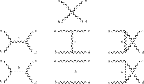
| (316) |
| (317) |
| (318) |
| (319) |
| (320) |
| (321) |
where
| (322) |
E.1.2 The high energy limit
When the gauge bosons are longitudinally polarized, the diagrams of figure 1 grow with energy for large center of mass energy . The most divergent behavior arises from the first four diagrams that grow like . To see this, one has to use the expression for the polarization vector for the longitudinal case, which is given by
| (323) |
To determine the coefficients of the high energy behavior (see eq. (333) below) we cannot use the approximate expression on the right-hand side of eq. (323) because we would then lose contributions from the terms that modify the terms. So we should use consistently the definitions of the left-hand side and expand the result in powers of , or . For instance, for particle we have,
| (324) |
and similarly for the other particles. Next we use the kinematics for the process
| (325) |
in order to write
| (326) | |||||
| (327) | |||||
| (328) | |||||
| (329) |
We then use these expressions to evaluate all the amplitudes. In the end we substitute in terms of the Mandelstam variable , through the relation
| (330) |
At this point all the amplitudes are expressed in terms of the Mandelstam variables and the masses. As the Mandelstam variables are not independent we can still use the relation
| (331) |
to express the result in terms of just two independent variables. Which ones should be used will depend on the problem. Next we want to isolate the terms that grow with and . To achieve this we make the scaling
| (332) |
and perform an expansion for small . The terms in are the coefficients of and the terms that grow like are the coefficients of . Therefore, we can write for each amplitude
| (333) |
where we assumed that the independent Mandelstam variables are and . We did this consistent expansion using FeynCalc and Mathematica for the Lorentz algebra and series expansion, respectively. To have an idea of what is involved we just write the exact amplitude for the s-channel exchange of a gauge boson:
| (334) |
This is a quite complicated expression, but making the series expansion as described above gives simply
| (335) |
If we had not taken the exact expression for the polarization vectors in eq. (323) but only the approximate expression, we would have obtained instead of eq. (E.1.2) the following expression,
| (336) |
which shows that the terms are correct but there is a difference in the terms as previously anticipated. Note that no such problem arises for the exchange of the scalars, as the most divergent terms are of order . Nevertheless we adopt the same procedure for all the diagrams.
The terms
The first four diagrams yield terms that grow like . To simplify the expressions we redefine the coefficients . The corresponding coefficients are given in table 5.
| Diagram | |||
The last line in this table is obtained after we use the relations found in ref. Cornwall:1974km and given in eq. (313). Namely,
| (337) | ||||
| (338) | ||||
| (339) |
where the antisymmetry of the constants was used. So the more divergent terms cancel only with the gauge part. The constraints that emerge simply imply that we must have a spontaneously broken gauge theory Cornwall:1974km ; LlewellynSmith:1973yud as given in eqs. (313)-(314).
The terms
Having shown that a spontaneously broken gauge theory assures that the the most divergent high energy behavior cancels, we consider next the terms that diverge like . Here the gauge theory part is not enough to achieve cancellation and we get constraints on the gauge boson couplings to scalars. For convenience we define
| (340) |
We also note that once we use eq. (E.1.2) there is no contribution at this order for .
| Diagram | ||
|---|---|---|
The results are summarized in table 6.
E.1.3 The sum rule of ref. Gunion:1990kf
To obtain the sum rule in eq. (2.4) of ref. Gunion:1990kf we take as independent the Mandelstam variables and . The coefficients of the terms growing with and must vanish. If we take the coefficient of we obtain the desired sum rule. To show this, we notice first that the sum of all contributions to is (sums implied)
| (341) | ||||
where we have defined . Now we use eqs. (337)–(339) to obtain
| (342) |
Inserting this result into eq. (E.1.3) we obtain,
| (343) |
Now we use the Jacobi identity of eq. (314) in the form
| (344) |
and subtract it from eq. (E.1.3). We then obtain the sum rule of eq. (2.4) of ref. Gunion:1990kf ,
| (345) |
where the prime in indicates that the sum only runs over massive gauge bosons.
E.1.4 Another sum rule
E.2 Sum Rules
E.2.1 The Amplitudes
The diagrams contributing to the scattering are given in figure 2.
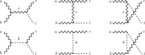
The corresponding amplitudes are
| (347) |
| (348) |
| (349) |
| (350) |
| (351) |
| (352) |
where
| (353) |
E.2.2 The high energy limit
In this case it is convenient to choose as independent variables and . The results are summarized in table 7. Again we used a definition similar to eq. (340),
| (354) |
| Diagram | ||
|---|---|---|
E.2.3 The sum rule of ref. Gunion:1990kf
To obtain the sum rule in eq. (2.5) of ref. Gunion:1990kf , we take as independent Mandelstam variables and . The coefficients of the terms growing with and must vanish. If we take the coefficient of we obtain the desired sum rule.
| (355) |
E.2.4 Another sum rule
If we take the coefficient of we get another sum rule,
| (356) |
which is just the crossed version of eq. (E.2.3).
E.3 Sum Rules
E.3.1 The Amplitudes
The diagrams contributing to the scattering are given in figure 3.
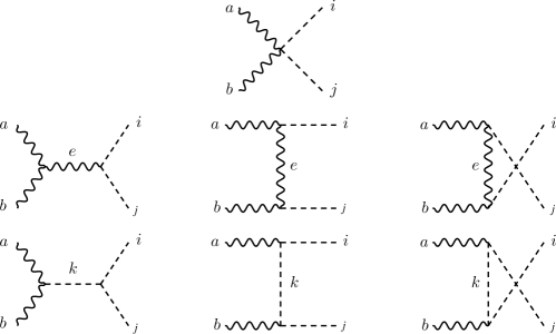
The diagram with the triple Higgs vertex does not exhibit any bad high energy behavior, and therefore one does not have to consider it here. The other amplitudes are
| (357) |
| (358) |
| (359) |
| (360) |
| (361) |
| (362) |
E.3.2 The high energy limit
In this case it is convenient to choose as independent variables and . The results are summarized in table 8. Again we used a definition similar to eq. (340),
| (363) |
| Diagram | ||
|---|---|---|
E.3.3 The sum rule of ref. Gunion:1990kf
To obtain the sum rule in eq. (2.6) of ref. Gunion:1990kf , we take as independent Mandelstam variables and . The coefficients of the terms growing with and must vanish. If we take the coefficient of we obtain the desired sum rule.
| (364) |
E.3.4 Another sum rule
If we take the coefficient of we get another sum rule,
| (365) |
which is just the crossed version of eq. (364).
Appendix F Proof that
Theories based on involve the operators
| (366) |
When acting on some neutral field,
| (367) |
The operators , and , when acting on a neutral () field , yield the corresponding eigenvalues , and , respectively. Thus,
| (368) | |||||
where there is an implicit sum running over all neutral fields in the theory, from to .222222Notice that nothing was assumed about the exact representations used, nor the value of . Thus,
| (369) |
and
| (370) |
We now turn to the cubic couplings. Using
| (371) |
we find
| (372) |
where . Substituting in eq. (368), we find the corresponding Feynman rules as
| (373) |
Defining the ratio of Feynman rules as
| (374) |
we get
| (375) |
One knows from experiment that to high precision rhoparm . Barring a fine tuning of the various vevs, that can only occur if all representations of the theory with scalar fields with non-vanishing vevs satisfy
| (376) |
Moreover, if eq. (376) is satisfied, then eq. (375) implies that is necessarily equal to . Note that this conclusion does not depend on whether the scalar potential is (or is not) CP-conserving.
References
- (1) G. Aad et al. [ATLAS Collaboration], Observation of a new particle in the search for the Standard Model Higgs boson with the ATLAS detector at the LHC, Phys. Lett. B 716 (2012) 1 [arXiv:1207.7214 [hep-ex]].
- (2) S. Chatrchyan et al. [CMS Collaboration], Observation of a new boson at a mass of 125 GeV with the CMS experiment at the LHC, Phys. Lett. B 716 (2012) 30 [arXiv:1207.7235 [hep-ex]].
- (3) G. Aad et al. [ATLAS and CMS Collaborations], Measurements of the Higgs boson production and decay rates and constraints on its couplings from a combined ATLAS and CMS analysis of the LHC pp collision data at and 8 TeV, JHEP 1608 (2016) 045 [arXiv:1606.02266 [hep-ex]].
- (4) See e.g., M. Drees and G. Gerbier, Dark Matter, in the 2016 Review of Particle Physics, in the 2016 Review of Particle Physics, C. Patrignani et al. [Particle Data Group], Chin. Phys. C 40 (2016) 100001.
- (5) See e.g., K. Nakamura and S.T. Petkov, Neutrino mass, mixing, and oscillations, in the 2016 Review of Particle Physics, C. Patrignani et al. [Particle Data Group], Chin. Phys. C 40 (2016) 100001.
- (6) See e.g., G.A. White, A Pedagogical Introduction to Electroweak Baryogenesis (IOP Publishing, Bristol, UK, 2016).
- (7) See , e.g., L. Susskind, The Gauge Hierarchy Problem, Technicolor, Supersymmetry, And All That, Phys. Rept. 104 (1984) 181.
- (8) See e.g., J. Erler and A. Freitas, Electroweak Model and constraints on New Physics, in the 2016 Review of Particle Physics, C. Patrignani et al. [Particle Data Group], Chin. Phys. C 40 (2016) 100001.
- (9) J.F. Gunion, H.E. Haber, G. Kane and S. Dawson, The Higgs Hunter’s Guide (Westview Press, Boulder, CO, 2000).
- (10) I. P. Ivanov, Building and testing models with extended Higgs sectors, Prog. Part. Nucl. Phys. 95 (2017) 160 [arXiv:1702.03776 [hep-ph]].
- (11) A. Barroso, P. M. Ferreira, R. Santos and J. P. Silva, Stability of the normal vacuum in multi-Higgs-doublet models, Phys. Rev. D 74 (2006) 085016 [hep-ph/0608282].
- (12) C. C. Nishi, The Structure of potentials with N Higgs doublets, Phys. Rev. D 76 (2007) 055013 [arXiv:0706.2685 [hep-ph]].
- (13) S. L. Glashow and S. Weinberg, Natural Conservation Laws for Neutral Currents, Phys. Rev. D 15 (1977) 1958.
- (14) E. A. Paschos, Diagonal Neutral Currents, Phys. Rev. D 15 (1977) 1966.
- (15) M.P. Bento, H.E. Haber, J.C. Romão and J.P. Silva, preprint in preparation.
- (16) C. H. Llewellyn Smith, High-Energy Behavior and Gauge Symmetry, Phys. Lett. 46B (1973) 233.
- (17) J. M. Cornwall, D. N. Levin and G. Tiktopoulos, Phys. Rev. D 10 (1974) 1145 [Erratum: Phys. Rev. D 11 (1975) 972].
- (18) H. A. Weldon, The Effects of Multiple Higgs Bosons on Tree Unitarity, Phys. Rev. D 30 (1984) 1547.
- (19) J. F. Gunion, H. E. Haber and J. Wudka, Sum rules for Higgs bosons, Phys. Rev. D 43 (1991) 904.
- (20) B. Grinstein, C. W. Murphy, D. Pirtskhalava and P. Uttayarat, Theoretical Constraints on Additional Higgs Bosons in Light of the 126 GeV Higgs, JHEP 1405 (2014) 083 [arXiv:1401.0070 [hep-ph]].
- (21) B. W. Lee, C. Quigg and H. B. Thacker, The Strength of Weak Interactions at Very High-Energies and the Higgs Boson Mass, Phys. Rev. Lett. 38 (1977) 883.
- (22) B. W. Lee, C. Quigg and H. B. Thacker, Weak Interactions at Very High-Energies: The Role of the Higgs Boson Mass, Phys. Rev. D 16 (1977) 1519.
- (23) H. Georgi and D. V. Nanopoulos, Suppression of Flavor Changing Effects From Neutral Spinless Meson Exchange in Gauge Theories, Phys. Lett. 82B, 95 (1979).
- (24) L. Lavoura, J. P. Silva, Fundamental CP violating quantities in a SU(2)U(1) model with many Higgs doublets, Phys. Rev. D 50 (1994) 4619.
- (25) G. C. Branco, L. Lavoura and J. P. Silva, CP Violation, (Oxford University Press, Oxford, UK, 1999).
- (26) S. Davidson and H. E. Haber, Basis-independent methods for the two-Higgs-doublet model, Phys. Rev. D 72 (2005) 035004 [Erratum: Phys. Rev. D 72 (2005) 099902].
- (27) H. E. Haber and D. O’Neil, Basis-independent methods for the two-Higgs-doublet model. II. The Significance of tan , Phys. Rev. D 74 (2006) 015018 [Erratum: Phys. Rev. D 74 (2006) 059905] [hep-ph/0602242].
- (28) F. J. Botella and J. P. Silva, Jarlskog-like invariants for theories with scalars and fermions, Phys. Rev. D 51, (1995) 3870.
- (29) C. C. Nishi, CP violation conditions in N-Higgs-doublet potentials, Phys. Rev. D 74 (2006) 036003 [Erratum: Phys. Rev. D 76 (2007) 119901] [hep-ph/0605153].
- (30) I. P. Ivanov and C. C. Nishi, Properties of the general NHDM. I. The Orbit space, Phys. Rev. D 82 (2010) 015014 [arXiv:1004.1799 [hep-th]].
- (31) M. Maniatis and O. Nachtmann, Stability and symmetry breaking in the general -Higgs-doublet model, Phys. Rev. D 92 (2015) 075017 [arXiv:1504.01736 [hep-ph]].
- (32) W. Grimus and L. Lavoura, Soft lepton flavor violation in a multi Higgs doublet seesaw model, Phys. Rev. D 66, (2002) 014016 [hep-ph/0204070].
- (33) W. Grimus, L. Lavoura, O. M. Ogreid and P. Osland, A Precision constraint on multi-Higgs-doublet models, J. Phys. G 35, (2008) 075001 [arXiv:0711.4022 [hep-ph]].
- (34) W. Grimus, L. Lavoura, O. M. Ogreid and P. Osland, The Oblique parameters in multi-Higgs-doublet models, Nucl. Phys. B 801 (2008) 81 [arXiv:0802.4353 [hep-ph]].
- (35) W. Grimus and H. Neufeld, Radiative Neutrino Masses in an SU(2)U(1) Model, Nucl. Phys. B 325 (1989) 18.
- (36) J. C. Romao and J. P. Silva, A resource for signs and Feynman diagrams of the Standard Model, Int. J. Mod. Phys. A 27 (2012) 1230025 [arXiv:1209.6213 [hep-ph]].
- (37) A. Djouadi, The Anatomy of electro-weak symmetry breaking. I: The Higgs boson in the standard model, Phys. Rept. 457 (2008) 1 [arXiv:hep-ph/0503172].
- (38) A. Djouadi, The Anatomy of electro-weak symmetry breaking. II. The Higgs bosons in the minimal supersymmetric model, Phys. Rept. 459 (2008) 1 [arXiv:hep-ph/0503173].
- (39) H. E. Haber and O. Stål, New LHC benchmarks for the -conserving two-Higgs-doublet model, Eur. Phys. J. C 75 (2015) 491 [Erratum: Eur. Phys. J. C 76 (2016) 312] [arXiv:1507.04281 [hep-ph]].
- (40) J. F. Gunion and H. E. Haber, Phys. Rev. D 67 (2003) 075019 [hep-ph/0207010].
- (41) H. G. J. Veltman, The Equivalence Theorem, Phys. Rev. D 41 (1990) 2294.
- (42) M. P. Bento, to appear.
- (43) A. Arhrib, Charged Higgs production through W-Higgs Fusion, talk given at the Workshop on Multi-Higgs Models, Lisboa, 6-9 September (2016).
- (44) A. Arhrib, K. Cheung, J. S. Lee and C. T. Lu, Enhanced charged Higgs production through W-Higgs fusion in W-b scattering JHEP 1605 (2016) 093 [arXiv:1509.00978 [hep-ph]].
- (45) I. F. Ginzburg and I. P. Ivanov, Tree level unitarity constraints in the 2HDM with CP violation, [hep-ph/0312374].
- (46) I. F. Ginzburg and I. P. Ivanov, Tree-level unitarity constraints in the most general 2HDM, Phys. Rev. D 72 (2005) 115010 [hep-ph/0508020].
- (47) S. Kanemura and K. Yagyu, Unitarity bound in the most general two Higgs doublet model, Phys. Lett. B 751 (2015) 289 [arXiv:1509.06060 [hep-ph]].
- (48) D. Das and U. K. Dey, Analysis of an extended scalar sector with symmetry, Phys. Rev. D 89 (2014) 095025 Erratum: [Phys. Rev. D 91 (2015) 039905] [arXiv:1404.2491 [hep-ph]].
- (49) M. Luscher and P. Weisz, Is There a Strong Interaction Sector in the Standard Lattice Higgs Model?, Phys. Lett. B 212 (1988) 472.
- (50) I. P. Ivanov and J. P. Silva, -conserving multi-Higgs model with irremovable complex coefficients, Phys. Rev. D 93 (2016) 095014 [arXiv:1512.09276 [hep-ph]].
- (51) P. M. Ferreira and J. P. Silva, Discrete and continuous symmetries in multi-Higgs-doublet models, Phys. Rev. D 78 (2008) 116007 [arXiv:0809.2788 [hep-ph]].
- (52) G.C. Branco, P.M. Ferreira, L. Lavoura, M.N. Rebelo, M. Sher and J.P. Silva, Theory and phenomenology of two-Higgs-doublet models, Phys. Rept. 516, (2012) 1 [arXiv:1106.0034 [hep-ph]].
- (53) I. F. Ginzburg, M. Krawczyk and P. Osland, Two Higgs doublet models with CP violation, [hep-ph/0211371].
- (54) A. Arhrib, E. Christova, H. Eberl and E. Ginina, CP violation in charged Higgs production and decays in the Complex Two Higgs Doublet Model, JHEP 1104 (2011) 089 [arXiv:1011.6560 [hep-ph]].
- (55) A. Barroso, P. M. Ferreira, R. Santos and J. P. Silva, Probing the scalar-pseudoscalar mixing in the 125 GeV Higgs particle with current data, Phys. Rev. D 86 (2012) 015022 [arXiv:1205.4247 [hep-ph]].
- (56) D. Fontes, J. C. Romão and J. P. Silva, in the complex two Higgs doublet model, JHEP 1412 (2014) 043 [arXiv:1408.2534 [hep-ph]].
- (57) A. W. El Kaffas, P. Osland and O. M. Ogreid, CP violation, stability and unitarity of the two Higgs doublet model, Nonlin. Phenom. Complex Syst. 10 (2007) 347 [hep-ph/0702097].
- (58) See the webpage at http://porthos.tecnico.ulisboa.pt/arXiv/C2HDM/.
- (59) See, e.g., appendix A.1.3 of Sergio Caracciolo, Alan D. Sokal and Andrea Sportiello, Algebraic/combinatorial proofs of Cayley-type identities for derivatives of determinants and pfaffians, Advances in Applied Mathematics 50 (2013) 474 [arXiv:1105.6270 [math.CO]].
- (60) J. Gallier and D. Xu, Computing exponentials of skew-symmetric matrices and logarithms of orthogonal matrices, Int. J. Robotics and Automation 17 (2002) 1.
- (61) H.K. Dreiner, H.E. Haber and S.P. Martin, Two-component spinor techniques and Feynman rules for quantum field theory and supersymmetry, Phys. Rept. 494 (2010) 1 [arXiv:0812.1594 [hep-ph]].
- (62) Andrew Baker, Matrix Groups: An Introduction to Lie Group Theory (Springer-Verlag, London, UK, 2002).
- (63) Francis D. Murnaghan, The Unitary and Rotation Groups (Spartan Books, Washington, DC, 1962).
- (64) L. F. Li, Group Theory of the Spontaneously Broken Gauge Symmetries, Phys. Rev. D 9 (1974) 1723.
- (65) V. Elias, S. Eliezer and A. R. Swift, Comment on ‘Group Theory of the Spontaneously Broken Gauge Symmetries’, Phys. Rev. D 12 (1975) 3356.
- (66) D. Wu, The Symmetry Breaking Pattern of Scalars in Low Dimension Representations, Nucl. Phys. B 199 (1982) 523 [Erratum: Nucl. Phys. B 213, (1983) 545].