Differential Distributions for t-channel Single Top-Quark Production and Decay at Next-to-Next-to-Leading Order in QCD

Abstract

We present a detailed phenomenological study of the next-to-next-to-leading order (NNLO) QCD corrections for $t$-channel single top (anti-)quark production and its semi-leptonic decay at the CERN Large Hadron Collider (LHC). We find the NNLO corrections for the total inclusive rates at the LHC with different center of mass energies are generally smaller than the NLO corrections, indicative of improved convergence. However, they can be large for differential distributions, reaching a level of $10\%$ or more in certain regions of the transverse momentum distributions of the top (anti-)quark and the pseudo-rapidity distributions of the leading jet in the event. In all cases the perturbative hard-scale uncertainties are greatly reduced after the NNLO corrections are included. We also show a comparison of the normalized parton-level distributions to recent data from the 8 TeV measurement of the ATLAS Collaboration. The NNLO corrections tend to shift the theoretical predictions closer to the measured transverse momentum distribution of the top (anti)-quark. Importantly, for the LHC at 13 TeV, we present NNLO cross sections in a fiducial volume with decays of the top quark included.

1 Introduction

The top quark ($t$) is the heaviest particle in the standard model (SM). To date, it has been observed at hadron colliders only through $t\bar{t}$ pair production or in single production. Single top quark production provides a great opportunity to directly probe the electroweak $Wtb$ vertex, which is otherwise difficult to measure. There are three single-production channels: the $t$-channel through the exchange of a spacelike $W$ boson, the $s$-channel through the exchange of a timelike $W$ boson, and associated production of $t$ with an on-shell $W$ boson. Since all three channels are directly connected to the $Wtb$ vertex, they can be used to measure the Cabibbo-Kobayashi-Maskawa (CKM) matrix element $V_{tb}$. Besides, they can be used to extract the top-quark mass Alekhin:2016jjz ; CMS:2016fdm or to constrain the ratio of $u$-quark to $d$-quark parton distributions 1404.7116 ; Alekhin:2015cza ; Berger:2016oht . Single top-quark production is also sensitive to physics beyond the SM hep-ph/0007298 , e.g., modified structure of $Wtb$ vertex, new gauge bosons or new heavy quarks, and top-quark flavor-changing neutral current, and so forth.

At a hadron collider such as the Fermilab Tevatron and CERN LHC, the dominant mechanism for single top-quark production is through $t$-channel exchange of a $W$ boson. This process was first observed at the Tevetron 0903.0885 ; 0903.0850 . At the LHC, the $t$-channel cross section has been measured by the ATLAS and CMS collaborations at $\sqrt{S}=7$ TeV 1106.3052 ; 1205.3130 ; 1209.4533 ; 1406.7844 , $\sqrt{S}=8$ TeV 1403.7366 ; 1702.02859 , and $\sqrt{S}=13$ TeV 1609.03920 ; 1610.00678 . Recently, differential distributions and fiducial cross section have also been measured 1702.02859 . The CKM matrix element $V_{tb}$ and the structure of the $Wtb$ vertex have been probed by ATLAS and CMS 1403.7366 ; 1510.03764 ; 1702.08309 . The polarization of top quark in $t$-channel production has also been measured 1511.02138 .

Significant efforts have been made to improve the theoretical description of single top quark production. The next-to-leading order (NLO) QCD corrections in the 5-flavor scheme are calculated in Refs. NUPHA.B435.23 ; hep-ph/9603265 ; hep-ph/9705398 ; hep-ph/9807340 ; hep-ph/0102126 ; hep-ph/0207055 ; Sullivan:2004ie ; hep-ph/0510224 ; 1007.0893 ; 1012.5132 . The NLO calculation in the 4-flavor scheme is carried out in Ref. 0903.0005 . Full NLO corrections including top quark leptonic decay are studied within the on-shell top-quark approximation hep-ph/0408158 ; hep-ph/0504230 ; 1012.5132 and beyond 1102.5267 ; 1305.7088 ; 1603.01178 . Code for fast numerical evaluation at NLO is provided in Ref. 1406.4403 . Soft gluon resummation is considered in Refs. 1010.4509 ; 1103.2792 ; 1210.7698 ; 1510.06361 . Matching NLO calculations to parton showers is done in the framework of POWHEG and MC@NLO Refs. hep-ph/0512250 ; 0907.4076 ; 1207.5391 ; 1603.01178 . For experimental analyses at the LHC, predictions from POWHEG or MC@NLO are used for modeling of the signal process in unfolding to parton level cross sections, as well as for comparison of data and theory. The cross sections from either measurement or prediction can have a theoretical uncertainty of about $5-10\%$ 1702.02859 . Predictions incorporating further higher-order or logarithmic corrections are desirable for precision measurements.

Next-to-next-to-leading order (NNLO) QCD corrections with a stable top quark are calculated in Refs. 1404.7116 ; Berger:2016oht , with neglect of certain subleading contributions in color, namely in the structure-function approximation. The calculation of Ref. Berger:2016oht also includes the top-quark leptonic decay at NNLO within the on-shell top-quark approximation. Thus for the first time a realistic parton-level simulation at NNLO is available. The NNLO QCD effects on experimental fiducial cross sections at 13 TeV are reported in Ref. Berger:2016oht . The corrections are found to be large, both from production and decay, owing mostly to the jet-veto condition in the definition of the fiducial volume. In this paper we provide further elaboration of the methods and numerical results of our NNLO calculation. We present NNLO results for the LHC at 7, 8, and 14 TeV, in particular the total inclusive cross sections and differential distributions with a stable top quark.

The rest of our paper is organized as follows. In Sec. 2, we expand upon our NNLO calculation presented in Ref. Berger:2016oht and its validation. In Sec. 3, we present our predictions for the total inclusive cross sections and the differential cross sections with a stable top-quark in the final state. Sec. 4 provides results on fiducial cross sections and distributions for which the top-quark decay is included through NNLO, enabling a more refined comparison with data. Readers interested principally in comparisons with experiment may chose to bypass Sec. 2 on a first reading of this paper. Finally our summary and conclusions are presented in Sec. 5. Our results show that the NNLO QCD corrections are large in certain regions of the differential distributions as well as for fiducial cross sections with jet veto selections. They stabilize the theoretical predictions, with residual scale variations of about one percent. The NNLO predictions provide an improved description of the transverse momentum distribution of the top quark measured by ATLAS collaboration.

2 Theoretical Framework

We describe in this section our calculation of single top-quark production and decay at hadron colliders through NNLO. The calculation for single antitop-quark production follows the same line of reasoning. Some of the results have been presented in our previous publication Berger:2016oht .

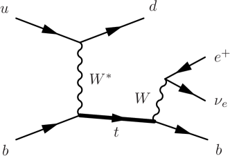
The LO Feynman diagram for the process under consideration is depicted in Fig. 1. We first discuss the approximations we employed to make the calculation feasible, namely, the on-shell top quark approximation hep-ph/9309234 ; hep-ph/9302311 and the structure-function approximation hep-ph/9705398 . Thanks to these approximations, the calculation effectively factors into three separate calculations with much simpler structure. We then present detailed formulas for these three simpler calculations. We discuss the validation of our calculation toward the end of this section.

Figure 1: The LO Feynman diagram for single top-quark production and decay at hadron colliders. Top quark is represented by a thick line. We show only one partonic channel in this figure.

2.1 On-shell top-quark approximation and structure-function approximation

In our calculation, we neglect interference between real radiation from the single top production stage and the top-quark decay stage. We also neglect a term in which there is a virtual gluon connecting the production and decay stages. This approximation is known as the on-shell top-quark approximation, i.e., the top quark is on its mass shell in all the diagrams when considered as an external state. For a generic inclusive enough infrared-safe observable, the omitted corrections are suppressed by the width of the top quark, $\Gamma_{t}/m_{t}$ hep-ph/9309234 ; hep-ph/9302311 . In the SM, top quark has a relatively small width but a large mass, $\Gamma_{t}/m_{t}<1\%$, an the approximation should provide an excellent representation of the full prediction. The on-shell approximation has been used in $t$-channel single top production by different groups NUPHA.B435.23 ; hep-ph/9705398 ; hep-ph/0207055 ; hep-ph/0504230 ; hep-ph/0408158 ; 1012.5132 at NLO, and recently at NNLO 1404.7116 ; Berger:2016oht . Effects beyond the on-shell approximation have been explored only at NLO thus far hep-ph/9603265 ; 1007.0893 , owing to the complexity of the calculation.

Through NNLO, the on-shell top-quark approximation can be written as

$$\sigma^{\rm LO}= \,\frac{1}{\Gamma^{(0)}_{t}}\mathrm{d}\sigma^{(0)}\otimes\mathrm{d}\Gamma^{(0)}_{t}{}$$

$$\delta\sigma^{\rm NLO}= \,\frac{1}{\Gamma^{(0)}_{t}}\left[\mathrm{d}\sigma^{(1)}\otimes\mathrm{d}\Gamma^{(0)}_{t}+\mathrm{d}\sigma^{(0)}\otimes\left(\mathrm{d}\Gamma^{(1)}_{t}-\frac{\Gamma^{(1)}_{t}}{\Gamma^{(0)}_{t}}\mathrm{d}\Gamma^{(0)}_{t}\right)\right]{}$$

$$\delta\sigma^{\rm NNLO}= \,\frac{1}{\Gamma^{(0)}_{t}}\left[\mathrm{d}\sigma^{(2)}\otimes\mathrm{d}\Gamma^{(0)}_{t}+\mathrm{d}\sigma^{(1)}\otimes\left(\mathrm{d}\Gamma^{(1)}_{t}-\frac{\Gamma^{(1)}_{t}}{\Gamma^{(0)}_{t}}\mathrm{d}\Gamma^{(0)}_{t}\right)\right.{}$$

$$\left.+\mathrm{d}\sigma^{(0)}\otimes\left(\mathrm{d}\Gamma^{(2)}_{t}-\frac{\Gamma^{(2)}_{t}}{\Gamma^{(0)}_{t}}\mathrm{d}\Gamma^{(0)}_{t}-\frac{\Gamma^{(1)}_{t}}{\Gamma^{(0)}_{t}}\left(\mathrm{d}\Gamma^{(1)}_{t}-\frac{\Gamma^{(1)}_{t}}{\Gamma^{(0)}_{t}}\mathrm{d}\Gamma^{(0)}_{t}\right)\right)\right],$$ (1)

where $\Gamma_{t}^{(0),(1),(2)}$ and $\sigma^{(0),(1),(2)}$ denote the Born, $\mathcal{O}(\alpha_{\scriptscriptstyle S})$, and $\mathcal{O}(\alpha_{\scriptscriptstyle S}^{2})$ top-decay width and production cross section, respectively. In Eq. (2.1) we have expanded the QCD corrections to both production and decay to the same order consistently. Equation (2.1) can be used for a fully differential calculation. After integrating over phase space, one reproduces the inclusive production cross section at a given order, as expected. For a correct treatment of spin correlations, the production cross section $\mathrm{d}\sigma$ and the decay width $\mathrm{d}\Gamma_{t}$ must be calculated for an on-shell polarized top quark. The symbol $\otimes$ denotes the appropriate summation over polarization.

Even with the on-shell top-quark approximation, the full NNLO QCD corrections to the production stage remain very difficult. For example, the full two-loop diagrams involve four different scales, the Mandelstam variables $s$ and $t$, the top quark mass $m_{t}$, and the $W$ boson mass $m_{\scriptscriptstyle W}$. A full two-loop amplitude of this complexity has not been obtained yet, either analytically or numerically, though interesting progress has been made 1409.3654 ; 1611.01087 . To bypass this complexity, we adopt the structure-function approximation hep-ph/9705398 , namely, we systematically neglect virtual and real radiation interference between the light quark line and the heavy quark line. These effects vanish exactly at NLO for squared amplitudes, owing to the traceless-ness of Gell-Mann matrices. This result can be seen from the color component of the real or virtual Feynman diagram for the NLO squared amplitudes with interference between the light and the heavy quark line, Fig. 2(a), which is proportional to $\mathrm{Tr}[t^{a}]\mathrm{Tr}[t^{a}]=0$. This result is true even for part of the NNLO diagrams, as long as there is only one gluon exchanged between the light and the heavy quark line, such as the diagram in Fig. 2(b). However, it ceases to be true for the diagrams with two gluons exchanged between the light and the heavy quark line, such as the diagram in Fig. 2(c). Such a diagram has a color factor $\mathrm{Tr}[t^{a}t^{b}]\mathrm{Tr}[t^{a}t^{b}]=(N_{c}^{2}-1)/4$, which is suppressed by a factor of $1/N_{c}^{2}$ compared with those without light quark and heavy quark line interference. In the structure-function approximation, such diagrams are neglected, in both virtual and a real corrections. These contributions are gauge invariant and IR finite by themselves, justifying the structure-function approximation. This approximation has been employed in the previous NNLO calculation for single top-quark production 1404.7116 ; Berger:2016oht . We note finally that the separation of single top-quark production into $t$-channel and $s$-channel terms could be ambiguous at NNLO, because there exist NNLO contributions which are the interference between one-loop $s$-channel and $t$-channel diagrams. These contributions fall into the class of two-gluon exchange diagrams in Fig. 2(c). These contributions are not present in the structure-function approximation, consistent with the use of $t$-channel in the title of this work.

((a))

((b))

((c))

Figure 2: Examples of the color component of NLO and NNLO Feynman diagrams for $t$-channel single top-quark production. Both virtual and real diagrams can be represented in this form. The lower loop represents the heavy-quark line, whereas the upper loop represents the light-quark line.

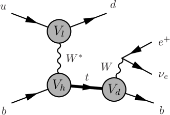
The on-shell top quark approximation and structure-function approximation can be summarized schematically in Fig. 3. Owing to these approximations, the full QCD corrections are factored into a piece describing the decay of the top quark, $V_{d}$, DIS-like production of the top quark, $V_{h}$, and the DIS-like production of a light jet, $V_{l}$. In the remainder of this section, we shall discuss the QCD corrections to each of these three parts separately.

Figure 3: Schematic diagram for $t$-channel single top-quark production at hadron colliders in the on-shell top quark approximation and the structure-function approximation. The full QCD corrections are factored into three different parts with these approximations.

2.2 QCD corrections for decay of the top quark

In this subsection we discuss the calculation of the fully differential semi-leptonic decay rate of a top quark through NNLO. These results were first presented in Ref. 1210.2808 . We provide more details here.

A typical QCD calculation beyond LO consists of virtual corrections, real emission corrections, and also mixed real-virtual corrections in the case of NNLO or beyond. A well-known feature of an on-shell perturbative QCD calculation is that individual piece of the higher order QCD corrections contains infrared divergences. The divergences cancel only in the sum of different contributions for infrared-safe observables. For example, the virtual corrections contain explicit infrared poles as a result of soft or collinear modes of the loop integrals. For real emission corrections, infrared poles result from integrating real radiation terms over unresolved phase space regions. These implicit poles in the corrections prevent a naive Monte-Carlo integral over the phase space in four space-time dimensions. A successful higher order QCD calculation requires the use of procedures to regulate the infrared singularities in the phase space integral.

In Ref. 1210.2808 , the phase space slicing method was employed to regulate the infrared singularities in the phase space integral. The idea of phase space slicing method is simple. For any infrared-safe observable $O$, the differential distribution can be written as

$$\frac{\mathrm{d}\sigma}{\mathrm{d}O}= \int^{\rho_{\rm cut}}_{0}\mathrm{d}\rho\,\frac{\mathrm{d}^{2}\sigma}{\mathrm{d}O\,\mathrm{d}\rho}+\int^{\rho_{\rm max}}_{\rho_{\rm cut}}\mathrm{d}\rho\,\frac{\mathrm{d}^{2}\sigma}{\mathrm{d}O\,\mathrm{d}\rho}{}$$

$$= \left.\frac{\mathrm{d}\sigma}{\mathrm{d}O}\right|_{\rm unres.}+\left.\frac{\mathrm{d}\sigma}{\mathrm{d}O}\right|_{\rm res.}\,,$$ (2)

where we have introduced a resolution variable $\rho$, and split the integral into an unresolved part, the first term on the RHS, and an resolved part, the second term on the RHS. There is no canonical definition for the resolution variable. The only requirement is that $\rho\to 0$ in the unresolved limit. In the resolved part, it is demanded that no phase space singularity be presented in the matrix element, and the integral can be performed in four dimensions using a Monte-Carlo method. The key idea of the phase space slicing method is that the QCD matrix element in the unresolved part can be approximated by the soft or collinear singular limit of the corresponding matrix element, known to have a universal factorized form. Owing to the simplicity of the QCD matrix element and phase space in the soft or collinear limit, it is sometimes possible to perform the unresolved phase space integral analytically. The infrared poles from the unresolved phase space integral can then be extracted in analytic form and cancelled against the corresponding infrared poles from the virtual corrections. The approximation in the unresolved part introduces an $\mathcal{O}(\rho_{\rm cut}\ln^{k}\rho_{\rm cut})$ error compared with the true calculation. To reduce this error as much as possible, and not modify the physical observable $O$ significantly, it is desirable to choose a small cut-off $\rho_{\rm cut}$ for the resolution variable. However, a small $\rho_{\rm cut}$ will also lead to a very steep integrand for the resolved part, and therefore potentially large Monte-Carlo integration uncertainty. Within the N-jettiness subtraction formalism 1504.02131 ; 1505.04794 , progress has been made recently in reducing the analytic error in the unresolved part by incorporating the leading logarithms of the power suppressed terms 1612.00450 ; 1612.02911 .

In Ref. 1210.2808 , the resolution variable is chosen as the inclusive jet mass, normalized to the top-quark mass,

$$\tau_{d}=\frac{(\sum_{i}p_{i})^{2}}{m_{t}^{2}}\,,$$ (3)

where the sum runs over all final-state QCD partons $p_{i}$. We use a subscript $d$ to denote the resolution variable chosen in the decay calculation. It is easy to see that $\tau_{d}$ satisfies the requirement for a good resolution variable for phase space slicing, namely $\tau_{d}\to 0$ when all the final-state QCD partons are either soft or collinear with each other.

We write the differential decay rate as

$$\frac{\mathrm{d}\Gamma_{t}}{\mathrm{d}O}= \int^{\tau_{d,\rm cut}}_{0}\mathrm{d}\tau_{d}\,\frac{\mathrm{d}^{2}\Gamma_{t}}{\mathrm{d}O\,\mathrm{d}\tau_{d}}+\int^{\tau_{d,\rm max}}_{\tau_{d,\rm cut}}\mathrm{d}\tau_{d}\,\frac{\mathrm{d}^{2}\Gamma_{t}}{\mathrm{d}O\,\mathrm{d}\tau_{d}}{}$$

$$= \left.\frac{\mathrm{d}\Gamma_{t}}{\mathrm{d}O}\right|_{\rm unres.}+\left.\frac{\mathrm{d}\Gamma_{t}}{\mathrm{d}O}\right|_{\rm res.}\,.$$ (4)

The task is to compute the unresolved part using an approximated QCD matrix element and phase space, and the resolved part using numerical Monte-Carlo integral. We stress that Eq. (2.2) holds for both the polarized and the unpolarized decay rate. Since our goal is to combine production and decay at NNLO, we compute the polarized decay rate in this work. For decay of the $W$ boson we adopt the narrow-width approximation. Therefore, we consider the decay of top quark to an on-shell $W$ boson and a $b$ quark at LO, while keeping the full polarization information for both the top quark and the $W$ boson. Because of the simple form of the resolution variable, the integrand of the unresolved part can be written in a convenient factorized form, up to error terms proportional to $\mathcal{O}(\ln^{k}\tau_{d})$ with $k_{s}\geq 0$,

$$\left.\frac{\mathrm{d}^{2}\Gamma_{t}}{\mathrm{d}O\,\mathrm{d}\tau_{d}}\right|_{\rm unres.}=\frac{\mathrm{d}\Gamma_{t}^{(0)}}{\mathrm{d}O}H_{d}(x,\mu)\int\mathrm{d}m^{2}\,\mathrm{d}k_{s}\,J(m^{2},\mu)S_{d}(k_{s},\mu)\delta\left(\tau_{d}-\frac{m^{2}+2E_{J}k_{s}}{m_{t}^{2}}\right)+\mathcal{O}(\ln^{k}\tau_{d})\,,$$ (5)

where $x=m_{\scriptscriptstyle W}^{2}/m_{t}^{2}$ characterizes the LO decay kinematics, and $E_{J}=(m_{t}^{2}-m_{\scriptscriptstyle W}^{2})/(2m_{t})$ is the energy of the $b$ jet at LO. Such a factorization formula was originally discussed in inclusive B decay in the end point region Korchemsky:1994jb ; Akhoury:1995fp ; Bauer:2003pi ; Bosch:2004th using Heavy Quark Effective Theory (HQET) and Soft-Collinear Effective Theory (SCET) hep-ph/0005275 ; hep-ph/0011336 ; hep-ph/0109045 ; hep-ph/0202088 . The same factorization formula can be used in top-quark decay since the observable is very similar, as long as its use is restricted to the perturbative region. Equation (5) indicates that in the unresolved region, the kinematic distributions for $O$ follow exactly those at LO. The normalization is determined in a factorization-friendly form in terms of a hard function $H_{d}(x,\mu)$, a jet function $J(m^{2},\mu)$, and a heavy-quark decay soft function $S_{d}(k_{s},\mu)$. The universality of infrared dynamics of QCD implies that these functions for top decay can also be extracted from those for inclusive B decay. Note that in Eq. (5), the polarization information of the top quark and the $W$ boson is encoded in the LO decay rate and the hard function only.

The hard function is related to the operator resulting from matching the heavy-to-light QCD form factor onto HQET and SCET. To leading power in the heavy quark limit and to all orders in $\alpha_{\scriptscriptstyle S}$, the operator can be expanded in terms of three basis functions,

$$\mathcal{O}_{tb}=C_{1}(x,\mu)\bar{\chi}_{n}\not{\varepsilon}(1-\gamma_{5})h+C_{2}(x,\mu)v\!\cdot\!\varepsilon\bar{\chi}_{n}(1+\gamma_{5})h+C_{3}(x,\mu)\frac{n\!\cdot\!\varepsilon}{n\!\cdot\!v}\bar{\chi}_{n}(1+\gamma_{5})h\,,$$ (6)

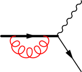
where $n^{\mu}=p_{b}^{\mu}/p_{b}^{0}$ and $v^{\mu}=p_{t}^{\mu}/m_{t}$ are the four-velocity of the $b$ jet and the top quark at LO in QCD; $\chi_{n}$ is the gauge-invariant collinear $b$ quark field; $h$ is the heavy top quark field; and $\varepsilon$ is the polarization vector for the $W$ boson. The Wilson coefficients $C_{i}(x,\mu)$ can be extracted from the QCD form factor calculation. For example, at one-loop, the relevant diagrams are shown in Fig. 4.

((a))

((b))

Figure 4: One-loop QCD form factor for heavy-to-light decay.

The Wilson coefficients $C_{i}(x,\mu)$ have been calculated through two loops for inclusive B decay Bonciani:2008wf ; Asatrian:2008uk ; Beneke:2008ei ; Bell:2008ws . The corresponding Wilson coefficients for top-quark decay can be simply read off from these studies. We quote the results through $\mathcal{O}(\alpha_{\scriptscriptstyle S})$ below,

$$C_{1}(x,\mu)= 1+\frac{\alpha_{\scriptscriptstyle S}}{4\pi}C_{F}\left(-2\ln^{2}\frac{\mu}{m_{t}}+4\ln\frac{\mu}{m_{t}}\log(1-x)-5\ln\frac{\mu}{m_{t}}+2\text{Li}_{2}(1-x)-2\log^{2}(1-x)\right.{}$$

$$\left.-\frac{\log(1-x)}{x}+3\log(1-x)+2\log(1-x)\log(x)-\frac{5\pi^{2}}{12}-6\right)+\mathcal{O}(\alpha_{\scriptscriptstyle S}^{2})\,,$$ (7)

$$C_{2}(x,\mu)= 0+\mathcal{O}(\alpha_{\scriptscriptstyle S}^{2})\,,$$ (8)

$$C_{3}(x,\mu)= \frac{\alpha_{\scriptscriptstyle S}}{4\pi}C_{F}\left(-\frac{2\log(1-x)}{x^{2}}-\frac{2}{x}+\frac{4\log(1-x)}{x}\right)+\mathcal{O}(\alpha_{\scriptscriptstyle S}^{2})\,.$$ (9)

We refer readers to Refs. Bonciani:2008wf ; Asatrian:2008uk ; Beneke:2008ei ; Bell:2008ws for the full two-loop results.

The hard function is defined as the squared matrix element of the effective operator normalized to the Born level result,

$$H_{d}(x,\mu)=\frac{\left|\langle Wb|\mathcal{O}_{tb}|t\rangle\right|^{2}}{\underset{\alpha_{\scriptscriptstyle S}\to 0}{\lim}\left|\langle Wb|\mathcal{O}_{tb}|t\rangle\right|^{2}}\,.$$ (10)

The soft function is defined as a vacuum matrix element of Wilson loops, which is independent of the top-quark spin. In a practical calculation, they can be obtained by taking the eikonal limit of the real corrections, with the insertion of a measurement function $\delta(k_{s}-k\!\cdot\!n)$, where $k_{s}$ is the total momentum of the soft radiation in the final state. For instance, the one-loop soft function is given by the integrals

$$S^{(1)}_{d}(k_{s},\mu)=\mu^{2\epsilon}\int\frac{\mathrm{d}^{4-2\epsilon}k}{(2\pi)^{4-2\epsilon}}(2\pi)\Theta(k^{0})\delta(k^{2})\delta(k_{s}-k\!\cdot\!n)\left|\parbox[h]{78.04842pt}{ \includegraphics[width=65.04034pt]{./eps/soft1.pdf} }+\parbox[h]{78.04842pt}{ \includegraphics[width=65.04034pt]{./eps/soft2.pdf} }\right|^{2}\,.$$ (11)

We use a double line to denote a timelike Wilson line, and a solid real line to denote a lightlike Wilson line. Note that the definition for the soft function is not Lorentz invariant. The violation of Lorentz invariance comes only from the measurement function $\delta(k_{s}-k\!\cdot\!n)$. The full two-loop soft function for inclusive B decay in the rest frame of a B meson has been computed in Ref. Becher:2005pd . The top quark decay soft function in the top quark rest frame is exactly the same as the B decay soft function, owing to universality of QCD amplitudes in the soft limit. We quote the result for the soft function through one loop below,

$$S_{d}(k,\mu)=\delta(k)+\frac{\alpha_{\scriptscriptstyle S}}{4\pi}C_{F}\left(-8\left[\frac{\ln(k/\mu)}{k}\right]_{\star}^{[k,\mu]}-4\left[\frac{1}{k}\right]_{\star}^{[k,\mu]}-\frac{\pi^{2}}{6}\delta(k)\right)+\mathcal{O}(\alpha_{\scriptscriptstyle S}^{2})\,,$$ (12)

where the star distribution is defined as

$$\int^{\mu}_{0}\mathrm{d}k\,[f(k)]_{\star}^{[k,\mu]}g(k)=\int^{\mu}_{0}\mathrm{d}k\,f(k)(g(k)-g(0))\,.$$ (13)

We refer to Ref. Becher:2005pd for the full two-loop soft function.

The jet function is defined as the vacuum matrix element of the gauge invariant collinear field with the insertion of a measurement function $\delta(m^{2}-p^{2})$, where $p^{2}$ is the virtuality of the collinear jet. In practice, it can be calculated by integrating the unintegrated splitting function with the above mentioned delta function inserted. At one-loop, the quark jet function is given by the integral

$$J(m^{2},\mu)=\mu^{2\epsilon}\int\frac{\mathrm{d}^{4-2\epsilon}l}{(2\pi)^{4-2\epsilon}}(2\pi)\Theta(l^{0})\delta(l^{2})\delta(m^{2}-p^{2})\left|\parbox[h]{78.04842pt}{ \includegraphics[width=65.04034pt]{./eps/jet1.pdf} }+\parbox[h]{78.04842pt}{ \includegraphics[width=65.04034pt]{./eps/jet2.pdf} }\right|^{2}\,.$$ (14)

We use a hatched diamond to denote collinear Wilson line in SCET. The jet function is completely factorized from the top quark, therefore also independent of top quark polarization. The overlap region of soft and collinear gluons is removed by the zero-bin subtraction procedure hep-ph/0605001 . For the inclusive jet function the zero-bin subtraction term vanishes to all orders in $\alpha_{\scriptscriptstyle S}$. The one-loop jet function is

$$J(m^{2},\mu)=\delta(m^{2})+\frac{\alpha_{\scriptscriptstyle S}}{4\pi}C_{F}\left(4\left[\frac{\ln(m^{2}/\mu^{2})}{m^{2}}\right]_{\star}^{[m^{2},\mu^{2}]}-3\left[\frac{1}{m^{2}}\right]_{\star}^{[m^{2},\mu^{2}]}+(7-\pi^{2})\delta(m^{2})\right)$$ (15)

For this work, we need the full two-loop quark jet function, which was computed in Ref. Becher:2006qw .

After putting the one-loop hard, soft, and jet functions together, one can derive the one-loop prediction for the unresolved integrand,

$$\left.\frac{\mathrm{d}^{2}\Gamma_{t}}{\mathrm{d}O\,\mathrm{d}\tau_{d}}\right|_{\rm unres.}= \frac{\mathrm{d}\Gamma_{t}^{(0)}}{\mathrm{d}O}\left\{\delta(\tau_{d})+\frac{\alpha_{\scriptscriptstyle S}}{4\pi}C_{F}\left[-4\left[\frac{\ln\tau_{d}}{\tau_{d}}\right]_{+}+\left(8\ln(1-x)-7\right)\left[\frac{1}{\tau_{d}}\right]_{+}\right.\right.{}$$

$$\left.\left.+\left(4\ln^{2}\frac{\mu}{m_{t}}-8\ln(1-x)\ln\frac{\mu}{m_{t}}+10\ln\frac{\mu}{m_{t}}-4\ln^{2}(1-x)+4\ln(1-x)\right.\right.\right.{}$$

$$\left.\left.\left.+7-\frac{7\pi^{2}}{6}+H_{d}^{(1)}(x,\mu)\right)\delta(\tau_{d})\right]\right\}+\mathcal{O}(\ln^{k}\tau_{d})\,,$$ (16)

where $[f(x)]_{+}$ is the usual plus distribution. The $\mu$ dependence cancels completely at this order, once the one-loop hard function is inserted. This is equivalent to the statement that the infrared divergences have been cancelled between virtual and real corrections at this order. Note that up to power corrections, the $\tau_{d}$ dependence of the unresolved integrand is very simple and can be integrated out readily in Eq. (2.2).

The factorized form of Eq. (5) is very convenient for calculations at higher order. Indeed, the only ingredients needed for a NNLO calculation of the unresolved part are the corresponding two-loop hard, jet, and soft functions, which are available from the previous precision study of inclusive B decay. This is one of the advantages of the phase space slicing method within the effective field theory framework, namely the convenient organization of different perturbative ingredients and the ease of recycling existing universal functions.

For a small cut-off $\tau_{d,\rm cut}$, integration of the unresolved distribution obtained from the factorization formula results in large logarithmic dependence on the cut-off. At NLO, the leading term scales as $\ln^{2}\tau_{d,\rm cut}$ as is evident from Eq. (15), whereas at NNLO it scales as $\ln^{4}\tau_{d,\rm cut}$. For sufficiently small cut-off, the large cut-off dependence is to be cancelled by the resolved contribution, up to Monte-Carlo integration uncertainty. The resolved contribution, as its name suggests, is free of infrared singularities at NLO. At NNLO, the resolved contribution contains sub-divergences. These sub-divergences cannot be resolved by our resolution variable $\tau_{d}$. They must be cancelled using other methods. Fortunately, the infrared structure of sub-divergences is lower by one order in $\alpha_{\scriptscriptstyle S}$ than the unresolved part. For a NNLO calculation, we can use any existing subtraction method to cancel the sub-divergences. In our calculation, we employ the dipole subtraction formalism hep-ph/9605323 with appropriate massive dipole terms Melnikov:2011qx to remove the sub-divergences. We also need the one-loop amplitudes for top quark decay to a $W$ plus two partons, and tree-level amplitudes for top decay to a $W$ plus three partons. We extract the former from Ref. Campbell:2005bb ; for the latter we use HELAS Murayama:1992gi .

2.3 QCD corrections for production of a single top quark: heavy quark line

Figure 5: LO diagram for single top quark production. We show only the part relevant for corrections associated with the heavy quark line. The thick solid line denotes the top quark. The wavy line denotes the off-shell $W$ boson that couples to the light quark line.

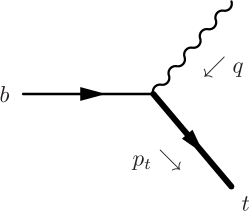
Having described decay of the top quark in the previous subsection, we turn now to QCD corrections associated with its production. In this subsection we treat the heavy quark line in the production process. In the structure-function approximation in which we work, the heavy quark part of LO process is represented by the diagram in Fig. 5. The light quark part is omitted in this step; it is treated in the next subsection. The light quark part (the upper vertex of Fig. 1 ) can be thought effectively as the DIS “leptonic” part that is invisible to the QCD corrections in the heavy quark line. The process now resembles charm-quark production in deep-inelastic neutrino scattering, for which NNLO QCD corrections were calculated in Ref. 1601.05430 . We note that the process in Fig. 5 is related by crossing to the top quark decay process we discuss in the previous section. Many of the ingredients in the last section can be used here.

Following the previous section, we define a resolution variable to isolate the unresolved part. As discussed in Ref. 1601.05430 , the appropriate resolution variable in this case is a fully inclusive version of beam thrust Stewart:2009yx or N-jettiness 1004.2489 ,

$$\tau_{h}=\frac{2\,p_{X}\!\cdot\!p_{n}}{m^{2}_{t}-q^{2}},\qquad\text{ with }p_{n}=\Big{(}\bar{n}\cdot(p_{t}-q)\Big{)}\frac{n^{\mu}}{2}\,.$$ (17)

It differs from the standard beam thrust or N-jettiness in that no partition is imposed in the phase space of final-state radiation, as there is only one collinear direction in the problem. This collinear direction is the beam (proton) direction associated with the bottom quark which enters the $Wtb$ vertex. In Eq. (17), $p_{X}$ is the momentum of total QCD radiation in the final state, and $p_{n}$ is a momentum aligned with the incoming beam whose large lightcone component equals the large lightcone component of the incoming momentum entering the $Wtb$ vertex. Here the lightcone direction $n$ is chosen as the direction of the incoming beam, and $\bar{n}=(1,-\vec{n})$, not to be confused with the jet direction used in the last section. Given the definition for $\tau_{h}$, the differential cross section for any infrared-safe observable $O$ can be separated into resolved and unresolved parts,

$$\frac{\mathrm{d}\sigma_{h}}{\mathrm{d}O}= \int^{\tau_{h,\rm cut}}_{0}\mathrm{d}\tau_{h}\,\frac{\mathrm{d}^{2}\sigma_{h}}{\mathrm{d}O\,\mathrm{d}\tau_{h}}+\int^{\tau_{h,\rm max}}_{\tau_{h,\rm cut}}\mathrm{d}\tau_{h}\,\frac{\mathrm{d}^{2}\sigma_{h}}{\mathrm{d}O\,\mathrm{d}\tau_{h}}{}$$

$$= \left.\frac{\mathrm{d}\sigma_{h}}{\mathrm{d}O}\right|_{\rm unres.}+\left.\frac{\mathrm{d}\sigma_{h}}{\mathrm{d}O}\right|_{\rm res.}\,.$$ (18)

We use the subscript “$h$” to denote that QCD corrections to the light quark line are neglected.

Similar to the case of top quark decay, we can write a factorization formula for the unresolved contribution, up to power corrections of the form $\tau_{h,\rm cut}\ln^{k}\tau_{h,\rm cut}$,

$$\left.\frac{\mathrm{d}\sigma_{h}}{\mathrm{d}O}\right|_{\rm unres.}= \int\mathrm{d}z\,\frac{\mathrm{d}\sigma_{h}^{(0)}(z)}{\mathrm{d}O}H_{h}(y,\mu)\int^{\tau_{h,\rm cut}}_{0}\mathrm{d}\tau_{h}\,\mathrm{d}t\,\mathrm{d}k_{s}\,B_{q}(t,z,\mu)S_{h}(k_{s},\mu){}$$

$$\cdot\delta\left(\tau_{h}-\frac{t+2k_{s}E_{b}}{m_{t}^{2}-q^{2}}\right)+\mathcal{O}(\tau_{h,\rm cut}\ln^{k}\tau_{h,\rm cut})\,,$$ (19)

where $E_{b}$ is the energy of the $b$ quark entering the $Wtb$ vertex. The derivation of this factorization formula is very similar to the derivation of beam thrust in N-jettiness factorization. In Eq. (2.3), $\mathrm{d}\sigma_{h}^{(0)}(z)/\mathrm{d}O$ is the Born level partonic differential cross section for the process

$$b(zP_{N})+W^{*}(q)\to t(p_{t})\,,$$ (20)

where $P_{N}$ is the momentum of the incoming hadron associated with the bottom quark. The definition of variable $y$ is $y=q^{2}/m_{t}^{2}<0$. The hard function for top quark production can be related through analytic continuation in a straightforward way to the hard function for top quark decay, defined in Eq. (10),

$$H_{h}(y,\mu)=H_{d}(y+i0,\mu)\,.$$ (21)

It is also possible to relate the heavy quark soft function to the decay soft function of Sec. 2.2. They both involve a timelike Wilson line and a lightlike Wilson line and a very similar measurement function. At one-loop the heavy quark soft function can be calculated from the diagrams

$$S^{(1)}_{h}(k_{s},\mu)=\mu^{2\epsilon}\int\frac{\mathrm{d}^{4-2\epsilon}k}{(2\pi)^{4-2\epsilon}}(2\pi)\Theta(k^{0})\delta(k^{2})\delta(k_{s}-k\!\cdot\!n)\left|\parbox[h]{78.04842pt}{ \includegraphics[width=65.04034pt]{./eps/heavysoft1.pdf} }+\parbox[h]{78.04842pt}{ \includegraphics[width=65.04034pt]{./eps/heavysoft2.pdf} }\right|^{2}\,,$$ (22)

where the lightlike direction $n$ points in the incoming beam direction. Comparing with Eq. (11), one may note that the timelike Wilson line has been crossed from the initial state to the final state, whereas the lightlike Wilson line from the final state to the initial state. This crossing leads only to a change of $\pm i\varepsilon$ to $\mp i\varepsilon$ in the Feynman prescription. The difference in the $i\varepsilon$ terms leads to a sign difference in the Glauber phase $\exp(\pm i\pi f(\epsilon))$ for the amplitudes, irrelevant at the cross section level.

We must also deal with frame dependence of the soft function. The frame dependence of the heavy quark soft function arises from the measurement function, $\delta(k_{s}-k\!\cdot\!n)$, just as for the decay soft function. Note that $k_{s}$ enters the observable through the combination $2E_{J}k_{s}$ for the top decay soft function, and $2E_{b}k_{s}$ for the heavy quark soft function. These combinations are Lorentz invariant, as we may see from writing the measurement function for top decay as

$$2E_{J}\delta(2E_{J}k_{s}-2k\!\cdot\!p_{b})\,,$$ (23)

and for heavy quark production as

$$2E_{b}\delta(2E_{b}k_{s}-2k\!\cdot\!p_{b})\,.$$ (24)

Therefore, we can choose to define the heavy quark soft function in the heavy quark rest frame, instead of the usual center of mass frame.

$$S_{h}(k_{s},\mu)=S_{d}(k_{s},\mu)\,,$$ (25)

in the heavy quark rest frame through all orders. Moreover,

$$E_{b}=\frac{m_{t}^{2}-q^{2}}{2m_{t}}$$ (26)

in the heavy quark rest frame. Now we can simply reuse the two-loop soft function of Ref. Becher:2005pd for our heavy-quark-line calculation.

The beam function is defined as the matrix element of a collinear field in a hadron state (proton in our case), with the virtuality $t=2p_{n}\!\cdot\!p_{c}$ of the measured beam jet Stewart:2009yx , where $p_{c}$ is the momentum of final state collinear radiation, and $p_{n}$ is defined in Eq. (17). The beam function can be written as the convolution of a perturbative coefficient function and the usual PDF,

$$B_{i}(t,x,\mu)=\sum_{j}\int\frac{\mathrm{d}\xi}{\xi}\,\mathcal{I}_{ij}\left(t,\frac{x}{\xi},\mu\right)f_{j}(\xi,\mu)+\mathcal{O}\left(\frac{\Lambda_{\rm QCD}^{2}}{t}\right)\,.$$ (27)

The one-loop quark-to-quark coefficient function can be calculated through the diagrams

$$\mathcal{I}_{qq}^{(1)}\left(t,z,\mu\right)= \int\frac{\mathrm{d}^{4-2\epsilon}l}{(2\pi)^{4-2\epsilon}}(2\pi)\Theta(l^{0})\delta(l^{2})\delta(t-2p_{n}\!\cdot\!l)\delta\big{(}l\!\cdot\!\bar{n}-(1-z)p_{n}\!\cdot\!\bar{n}\big{)}{}$$

$$\times\left|\parbox[h]{121.41306pt}{ \includegraphics[width=108.405pt]{./eps/beam1.pdf} }+\parbox[h]{121.41306pt}{ \includegraphics[width=108.405pt]{./eps/beam2.pdf} }\right|^{2}\,.$$ (28)

We also need the gluon-to-quark coefficient function at this order. The quark beam function has been calculated through two loops 1401.5478 . We quote the result to one-loop here

$$\mathcal{I}_{qq}(t,z,\mu)= \delta(t)\delta(1-z)+\frac{\alpha_{\scriptscriptstyle S}}{2\pi}C_{F}\left\{2\left[\frac{\ln(t/\mu^{2})}{t}\right]_{\star}^{[t,\mu^{2}]}\delta(1-z)+\left[\frac{1}{t}\right]_{\star}^{[t,\mu^{2}]}\frac{(1+z^{2})}{[1-z]_{+}}\right.{}$$

$$\left.+\delta(t)\left[\frac{(1+z^{2})}{[1-z]_{+}}-\frac{\pi^{2}}{6}\delta(1-z)+\left(1-z-\frac{1+z^{2}}{1-z}\ln z\right)\right]\right\}+\mathcal{O}(\alpha_{\scriptscriptstyle S}^{2})\,,{}$$

$$\mathcal{I}_{qg}(t,z,\mu)= \frac{\alpha_{\scriptscriptstyle S}}{2\pi}T_{F}\left\{\left[\frac{1}{t}\right]_{\star}^{[t,\mu^{2}]}(1-2z+2z^{2})+\delta(t)\left[(1-2z+2z^{2})\left(\ln\frac{1-z}{z}-1\right)+1\right]\right\}{}$$

$$+\mathcal{O}(\alpha_{\scriptscriptstyle S}^{2})\,.$$ (29)

After substituting the expansion of hard, soft, and beam functions into the factorization formula in Eq. (2.3), one obtains the unresolved distribution to leading power in $\tau_{h}$. Again, the dependence on $\tau_{h}$ is very simple and can be integrated analytically.

The calculation for the resolved contribution follows closely the decay calculation in Sec. 2.2. In fact, all the matrix elements can be recycled from the last section. Again, we use dipole subtraction to remove those sub-divergences which cannot be resolved by $\tau_{h}$.

2.4 QCD corrections for production of a single top quark: light quark line

For the QCD corrections associated with the light-quark line (the upper vertex of Fig. 1 ), we adopt the method of “Projection-to-Born” in Ref. 1506.02660 . The key ingredients in this approach are the inclusive NNLO DIS coefficient functions vanNeerven:1991nn ; Zijlstra:1992qd ; Zijlstra:1992kj , for which a conveniently parametrized version is available vanNeerven:1999ca ; vanNeerven:2000uj . The hadronic tensor can be expressed in terms of three scalar form factors 1109.3717

$$W_{\mu\nu}(x,Q^{2})=(-g_{\mu\nu}+\frac{q_{\mu}q_{\nu}}{q^{2}})F_{1}(x,Q^{2})+\frac{\hat{P}_{\mu}\hat{P}_{\nu}}{P\cdot q}F_{2}(x,Q^{2})+i\epsilon_{\mu\nu\alpha\beta}\frac{P^{\alpha}q^{\beta}}{2P\cdot q}F_{3}(x,Q^{2})\,.$$ (30)

Here $P$ is the momentum of the incident proton at the light-quark vertex, $q$ is the momentum transfer carried by the virtual $W$ boson, $\epsilon_{\mu\nu\alpha\beta}$ is the completely antisymmetric tensor, $Q^{2}=-q^{2}$, and Bjorken variable $x=Q^{2}/2P\cdot Q$. The momentum $\hat{P}$ is defined as

$$\hat{P}_{\mu}=P_{\mu}-\frac{P\cdot q}{q^{2}}q_{\mu}\,.$$ (31)

$F_{i}$ are structure functions for charged-current DIS which can be expressed as convolutions of the parton distributions and the DIS coefficient functions. In our case both $x$ and $q$ can be determined by kinematics at the heavy-quark vertex. By contracting this hadronic tensor with the squared matrix element for the heavy-quark vertex, keeping phase space unintegrated for the top quark, we can calculate the total cross sections and differential distributions of the top quark. This procedure is similar to the NNLO calculations of Higgs boson production via vector boson fusion in the double DIS approximation 1003.4451 .

The method of “Projection-to-Born” was used later in Ref. 1506.02660 to retain the jet activity at the light-quark vertex and applied to Higgs boson production. The spirit of the method is illustrated in Fig. 6.

Figure 6: Schematic diagrams of the “Projection-to-Born” method, including the inclusive contributions, followed by separate contributions from the double-unresolved region, the single-unresolved region, and the fully-resolved region.

The full NNLO corrections can be separated into contributions from the double-unresolved region, single-unresolved region, and fully-resolved region depending on the phase space of real radiation, as sketched in the last three diagrams in Fig. 6. Expressions for diagrams (c) and (d) can be obtained from the NLO results for processes with one more hard radiation at Born level, similar to the phase space slicing method. For the remaining contributions from the double-unresolved region, diagram (b), expressions can be obtained by subtracting diagrams (c) and (d) from the inclusive results represented by diagram (a). Furthermore, since all radiation is unresolved there, the final state jet has Born-like kinematics and is uniquely determined by $x$ and $q$. In practice, by a rearrangement of the different pieces, the final results consist of two components. First is the NNLO structure function contribution from Eq. (30) with Born-like kinematics determined by $x$ and $q$. Second is the contribution from 2-jet production at NLO supplemented by a counter-term contribution. The counter-term is constructed in such a way that for every event in the Monte Carlo integration of the 2-jet NLO piece, a counter-event is generated with opposite weight and with Born-like kinematics determined by $x$ and $q$. The counter-events remove contributions from the resolved region in the inclusive structure functions, as well as make the NLO calculation numerically stable. For the real-virtual corrections needed for the 2-jet NLO calculation, we extracted the one-loop helicity amplitudes from DIS 2 jet production in Ref. 0904.2665 .

2.5 Validation of the calculation

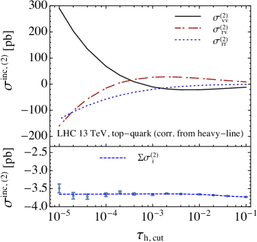
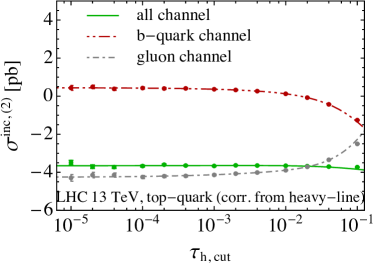
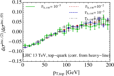
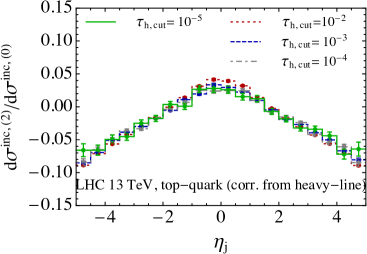
In the phase-space slicing method, we check the stability of various analytical expressions as well as the numerical implementations under variation of the small cut-off parameter. We should expect the results to converge smoothly to the true NNLO corrections after large cancellations of individual pieces. We demonstrate the cancellations for the heavy-quark line in Fig. 7 for the case of NNLO corrections to the total inclusive cross sections. In the upper panel we show three contributions to the NNLO corrections: the below-cut-off unresolved contribution $\sigma_{VV}^{(2)}$, the real-virtual part of the resolved contribution $\sigma_{RV}^{(2)}$, and double-real parts of the resolved contribution $\sigma_{RR}^{(2)}$. The individual contributions vary considerably with $\tau_{h,\rm cut}$, but the total contribution, shown in the lower panel, is stable and converges to a stable NNLO correction when $\tau_{h,\rm cut}$ is small. The cancellation of the three pieces is about one part out of a hundred. One may notice that the power corrections are rather small even for $\tau_{h,\rm cut}$ as large as $10^{-1}$. This small overall power correction results from an accidental cancellation of the power corrections from different partonic channels at large $\tau_{h,\rm cut}$, as shown in Fig. 8. Results for the $b$-quark and the gluon channel show considerable dependence on the cutoff when $\tau_{h,\rm cut}\sim 10^{-1}$. However these power corrections have a different sign and cancel largely in the sum. In Fig. 9 we examine the dependence on the cut-off in the differential distributions without decay. We show the transverse momentum of the stable top quark and the pseudorapidity of the leading jet. The corrections are normalized to the LO distributions. The error bars represent the estimated statistical uncertainties from the numerical integration. There is good agreement of the results when the cut-off is small. In practice we find optimal values of $\tau_{h,\rm cut}$ at about $10^{-4}\sim 10^{-3}$ where the power corrections are negligible and numerical integration stability is preserved.

Figure 7: Various components of the NNLO corrections from the heavy-quark line for the total inclusive cross section as a function of the cut-off, for single top-quark production at 13 TeV.

Figure 8: Cut-off dependence of different partonic channel contributions at NNLO from the heavy-quark line for the total inclusive cross section for top-quark production at 13 TeV.

Figure 9: NNLO corrections from the heavy-quark line for the transverse momentum distribution of the top quark (left), and the pseudorapidity distribution of the leading jet (right), for top-quark production at 13 TeV, with different choices of the cut-off.

For the resolved parts of all three NNLO calculations, we have cross checked our implementations with Gosam 1404.7096 and Sherpa 0811.4622 and found full agreement. The code for the calculation involving top-quark decay is based on our previous one used for calculation of the differential width 1210.2808 . An independent calculation based on a different infrared subtraction method was performed in Ref. 1301.7133 , and it confirms our results. We also checked explicitly that if we do not apply any selection cut, the NNLO corrections from decay do not change the total event rate in our numerical calculation, as expected from Eq. (2.1). For implementation of the structure functions needed for the calculation of light-quark line, we have compared our results with APFEL 1310.1394 and found good agreement. To compare our results with those in Ref. 1404.7116 for the case of a stable top (anti-)quark, we calculated the NNLO total inclusive cross sections at 8 TeV using the same choices of parameters. We found a difference of $\sim 1\%$ on the NNLO cross sections. With a refined comparison through private communications, we traced the source of this discrepancy to NNLO contributions associated with the heavy-quark line, with the $b$-quark initial state. All other parts in the NNLO corrections and all parts of the NLO contributions agree between the two results within numerical uncertainties. It has not been possible to further pin down the differences. We leave this issue for possible future investigation.

In calculations of the fiducial cross sections we also need a theoretically well-defined flavor-jet algorithm for the $b$-quark jet. At the parton level, the definition of a $b$-quark jet has some level of ambiguity. Naively, the $b$-jet can be defined as a conventional jet whose total $b$-flavor number is non-zero (counting the $b$ quark with $b$-flavor number $1$, and $b$ anti-quark with $b$-flavor number $-1$). However, the resulting jet cross section is not infrared safe in the zero-mass case. In a partonic configuration in which a soft gluon splits into a $b\bar{b}$ pair with large separation angle, the a $b$ quark may be clustered with other hard radiation and identified as a $b$-quark jet. A modification of the $k_{T}$ algorithm to address the IR safety problem of a $b$-quark jet is proposed in 0704.2999 . However, current experimental measurements of single top-quark production at the LHC use the anti-$k_{T}$ algorithm 0802.1189 . We do not adopt the flavor-jet algorithm in 0704.2999 . In our NNLO corrections, the specific configurations which can lead to infrared safety issues appear in the diagrams shown in Fig. 10.

Figure 10: Feynman diagrams with a soft gluon splitting into a $b\bar{b}$ pair, for NNLO corrections at the light-quark line, the heavy-quark line, and the top quark decay, respectively. The green fermion line represents a $b$ quark or anti-quark.

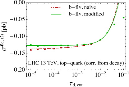
In the first two diagrams, the splitting does not involve the primary $b$ quark from decay of the top quark. We simply assign a zero $b$-flavor number for the bottom (anti-)quark in this splitting while keeping a non-zero $b$-flavor number for the primary $b$ quark. For the case of top quark decay there can be two $b$ quarks and one $b$ anti-quark in the final state, as shown by the third diagram. In this case we first find a pair of $b$ quarks and an anti-quark, computing the invariant masses of the two $b{\bar{b}}$ pairs. Then we assign a zero $b$-flavor number for each $b/{\bar{b}}$ quark in the pair with the smaller invariant mass and a non-zero $b$-flavor number for the other $b$ quark. After combining this modified flavor assignment with the anti-$k_{T}$ jet algorithm, one can verify the infrared safety of our NNLO cross sections. An interesting test of infrared safety is made by checking the dependence of the cross sections on the cut-off parameter. In Fig. 11 we show the NNLO corrections from top-quark decay on the fiducial cross section, as a function of the cut-off $\tau_{d,\rm cut}$. We can see the incomplete cancellation of cut-off dependence with the naive flavor assignment, an indication of infrared problems of the algorithm. In the modified case we observe convergence similar to that in Fig. 8.

Figure 11: NNLO correction from top-quark decay on the fiducial cross section as a function of the cut-off, for top-quark production at 13 TeV. Error bars represent a scan over different cut-off values. The curves show fits to the points in the small cut-off region for two different flavor assignments.

3 Cross sections and distributions for a stable top quark

In this section we present predictions for the total inclusive cross sections and differential cross sections for a top quark treated as an observable stable object. The parameters used in our numerical calculations are listed here. We use a top quark mass of 172.5 GeV and a $W$ boson mass of 80.385 GeV. We choose $|V_{tb}|=1$, $G_{F}=1.166379\times 10^{-5}{\rm GeV}^{-2}$ and the CT14 parton distribution functions (PDFs) Dulat:2015mca with $\alpha_{s}(M_{Z})=0.118$. We specify below which perturbative order we use for the PDFs (LO, NLO, NNLO). The nominal perturbative hard-scale choice is $\mu_{R}=\mu_{F}=m_{t}$ with scale uncertainty evaluated by varying the two together over the range $0.5<\mu/\mu_{o}<2$.

3.1 Total inclusive cross section

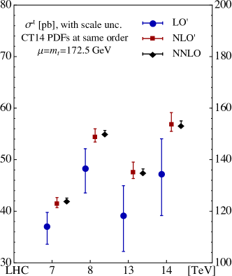
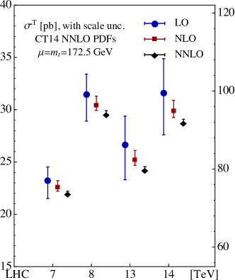
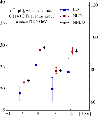
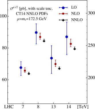
In Fig. 12 we plot the total inclusive cross sections for single top-quark production at the LHC with different energies. For 7 and 8 TeV, the scale of cross sections is shown on the left-vertical axis; for 13 and 14 TeV the scale on the right-vertical axis is appropriate. The predictions in the left side of Fig. 12 are obtained with CT14 NNLO PDFs throughout even though the hard matrix elements are computed at LO, NLO, and NNLO respectively. The QCD corrections are negative when the same PDFs are used. The NNLO corrections are about $2\sim 3$% in general compared to $3\sim 5$% at NLO. The error bars represent perturbative scale variations at different orders. Scale variations are reduced by a factor of about 3 after the NNLO corrections are included. The remaining uncertainties are generally at a level of one percent at NNLO, e.g., +1.0% and -0.6% for top quark production at 13 TeV and +1.1% and -0.5% for top anti-quark production. The predictions shown in the plot on the right side of Fig. 12 are obtained with CT14 PDFs at the associated orders, meaning with LO PDFs for LO predictions and so on. In this case the LO predictions drop significantly owing to the relatively smaller bottom-quark PDFs from one-loop QCD evolution. The NNLO corrections are small possibly because the process studied consists of similar components as for the deep inelastic scattering (DIS) process used for determination of PDFs. Thus it is expected that at least part of the QCD effects have been absorbed into the fitting of PDFs. Figure 13 shows results for top anti-quark production at the LHC. Conclusions concerning the size of QCD corrections and scale variations are similar to those for the top quark.

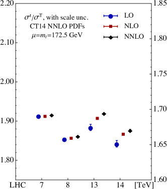
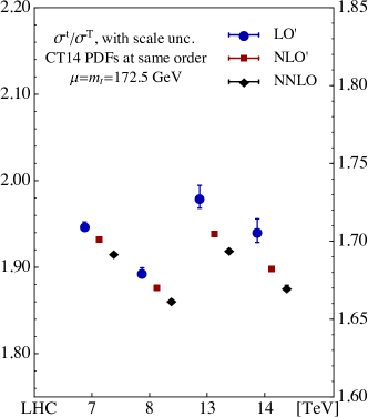
We display the sum and ratio of the top quark and anti-quark production cross sections in Fig. 14 and Fig. 15, for 7 and 8 TeV with the scale on left-vertical axis, and 13 and 14 TeV with the scale on right-vertical axis. In both figures the scale variations are calculated by setting scales in top quark and anti-quark production be the same and changing them simultaneously. The behavior can be understood inasmuch as the QCD corrections in top quark and anti-quark production are strongly correlated, as shown in Figs. 12 and 13. The cross section ratios in Fig. 15 are rather stable against QCD corrections. They change by at most 1% from LO to NNLO if the same PDFs are used. The differences induced by PDFs at different orders are larger than the QCD corrections in general. For completeness we provide numerical values of predictions with CT14 NNLO PDFs in Table 1.

Figure 12: Inclusive cross sections for $t$-channel single top quark production at LO, NLO and NNLO with CT14 NNLO PDFs (left) and CT14 PDFs at same order (right), at the LHC with different center of mass energies. Error bars represent scale uncertainties obtained by varying the renormalization and factorization scale from $\mu_{F}=\mu_{R}=m_{t}/2$ to $2m_{t}$.

Figure 13: Inclusive cross sections for $t$-channel single top anti-quark production, similar to Fig. 12.

Figure 14: Sum of inclusive cross sections for $t$-channel single top quark and anti-quark production, similar to Fig. 12.

Figure 15: Ratio of inclusive cross sections for $t$-channel single top quark and anti-quark production, similar to Fig. 12.

inclusive		LO	NLO	NNLO
7 TeV	$\sigma(t)\,{\rm[pb]}$	$44.55_{-7.5\%}^{+5.3\%}$	$43.14_{-1.6\%}^{+2.9\%}$	$42.05_{-0.6\%}^{+1.2\%}$
	$\sigma(\bar{t})\,{\rm[pb]}$	$23.29_{-7.6\%}^{+5.3\%}$	$22.57_{-1.5\%}^{+2.9\%}$	$21.95_{-0.7\%}^{+1.2\%}$
	$\sigma(t+\bar{t})\,{\rm[pb]}$	$67.84_{-7.6\%}^{+5.3\%}$	$65.71_{-1.6\%}^{+2.9\%}$	$64.00_{-0.6\%}^{+1.2\%}$
	$\sigma(t)/\sigma(\bar{t})$	$1.913_{-0.1\%}^{+0.1\%}$	$1.912_{-0.1\%}^{+0\%}$	$1.916_{-0\%}^{+0.1\%}$
8 TeV	$\sigma(t)\,{\rm[pb]}$	$58.41_{-8.1\%}^{+5.9\%}$	$56.46_{-1.6\%}^{+2.9\%}$	$55.01_{-0.6\%}^{+1.2\%}$
	$\sigma(\bar{t})\,{\rm[pb]}$	$31.52_{-8.3\%}^{+6.0\%}$	$30.41_{-1.6\%}^{+2.9\%}$	$29.55_{-0.6\%}^{+1.2\%}$
	$\sigma(t+\bar{t})\,{\rm[pb]}$	$89.93_{-8.2\%}^{+5.9\%}$	$86.87_{-1.6\%}^{+2.9\%}$	$84.57_{-0.6\%}^{+1.2\%}$
	$\sigma(t)/\sigma(\bar{t})$	$1.854_{-0.1\%}^{+0.1\%}$	$1.856_{-0.1\%}^{+0\%}$	$1.861_{-0\%}^{+0.1\%}$
13 TeV	$\sigma(t)\,{\rm[pb]}$	$144.5_{-10\%}^{+8.1\%}$	$138.8_{-1.7\%}^{+2.9\%}$	$135.1_{-0.6\%}^{+1.0\%}$
	$\sigma(\bar{t})\,{\rm[pb]}$	$86.34_{-10\%}^{+8.3\%}$	$82.28_{-1.6\%}^{+3.0\%}$	$79.73_{-0.5\%}^{+1.1\%}$
	$\sigma(t+\bar{t})\,{\rm[pb]}$	$230.9_{-10\%}^{+8.2\%}$	$221.1_{-1.7\%}^{+3.0\%}$	$214.8_{-0.6\%}^{+1.0\%}$
	$\sigma(t)/\sigma(\bar{t})$	$1.674_{-0.2\%}^{+0.3\%}$	$1.687_{-0.1\%}^{+0\%}$	$1.694_{-0.1\%}^{+0\%}$
14 TeV	$\sigma(t)\,{\rm[pb]}$	$164.4_{-10\%}^{+8.4\%}$	$157.8_{-1.7\%}^{+3.0\%}$	$153.3_{-0.5\%}^{+1.1\%}$
	$\sigma(\bar{t})\,{\rm[pb]}$	$99.60_{-11\%}^{+8.7\%}$	$94.77_{-1.6\%}^{+3.0\%}$	$91.81_{-0.5\%}^{+1.0\%}$
	$\sigma(t+\bar{t})\,{\rm[pb]}$	$264.0_{-11\%}^{+8.5\%}$	$252.5_{-1.7\%}^{+3.0\%}$	$245.1_{-0.5\%}^{+1.1\%}$
	$\sigma(t)/\sigma(\bar{t})$	$1.651_{-0.2\%}^{+0.3\%}$	$1.665_{-0.1\%}^{+0\%}$	$1.670_{-0\%}^{+0.1\%}$

Table 1: Inclusive cross sections and their ratio for $t$-channel single top (anti-)quark production at LO, NLO and NNLO with CT14 NNLO PDFs at the LHC with different center of mass energies. Scale uncertainties are obtained by varying the renormalization and factorization scale from $\mu_{F}=\mu_{R}=m_{t}/2$ to $2m_{t}$.

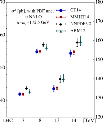
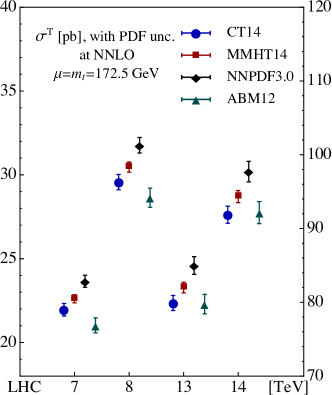
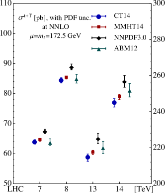
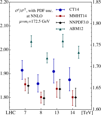
We show dependence of the total inclusive cross sections and their ratios on different choices of PDFs in Figs. 16 and 17, all calculated at NNLO and with NNLO PDFs. The PDFs sets include CT14 Dulat:2015mca , MMHT2014 Harland-Lang:2014zoa , and NNPDF3.0 Ball:2014uwa , all with $\alpha_{s}(M_{Z})=0.118$, and ABM12 Alekhin:2013nda with the default $\alpha_{s}(M_{Z})$ values. The error bars represent the $1\,\sigma$ PDF uncertainties of individual groups. The MMHT2014 results have the smallest PDF uncertainties among all groups. The spread of predictions from different PDFs are especially large for the top anti-quark production. The spread can reach more than 10%, as shown by differences of the ABM12 and NNPDF3.0 predictions, amounting to deviations of about $3\sigma$, even if both error estimates are taken into account. The discrepancies are even more pronounced in predictions of the cross section ratios as shown in Fig. 17. The ABM12 PDFs yield a much higher ratio compared to other three groups. Precise measurements of the cross section ratio from the LHC Run 2 can further differentiate among these PDFs.

Figure 16: Inclusive cross sections for $t$-channel single top quark (left) and anti-quark (right) production at NNLO with various NNLO PDFs, for the LHC with different center of mass energies. Error bars represent $1\,\sigma$ PDF uncertainties.

Figure 17: Sum (left) and ratio (right) of inclusive cross sections for $t$-channel single top quark and anti-quark production, similar to Fig. 16.

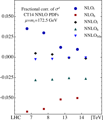
In Fig. 18 we show the fractional QCD corrections of different gauge invariant pieces, including contributions from the light-quark line, the heavy-quark line, and products of the two. The latter starts at NNLO. We observe cancellations of QCD corrections from the light and the heavy-line, driving the full corrections to moderate negative values. The contributions from the heavy-quark line dominate the NNLO corrections, while contributions from the light-quark vertex and the products are almost negligible.

Figure 18: Fractional corrections for the inclusive cross sections of $t$-channel single top quark and anti-quark production at NLO and NNLO at the LHC with different center of mass energies, computed with CT14 NNLO PDFs, and separated into component contributions.

3.2 Stable top quark differential cross sections

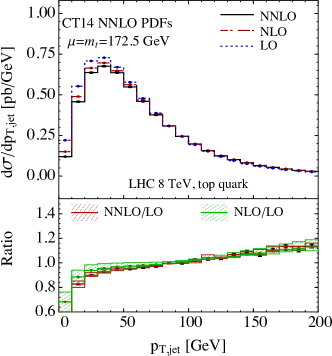
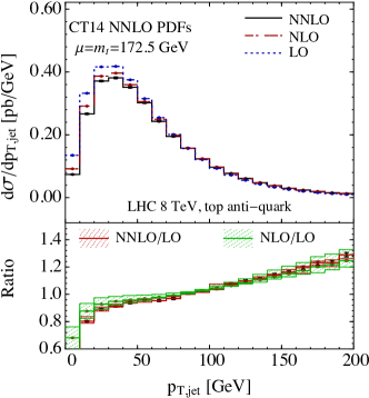
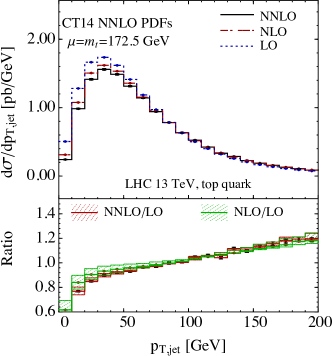
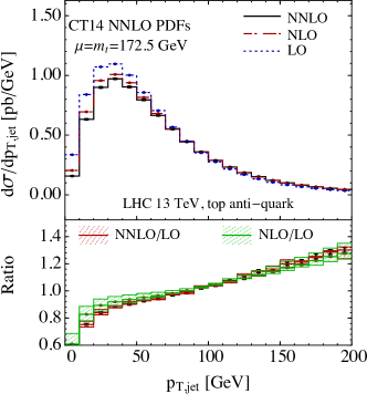
We present transverse momentum distributions of the top quark and anti-quark at 8 and 13 TeV in Fig. 19. We show the distributions at various orders in the upper panel, and the ratios of NLO and NNLO predictions to the LO ones in the lower panel, with scale variations. The QCD corrections can be negative or positive, depending on values of the transverse momentum, and are smallest near 70 GeV. The corrections are especially large in the regions of low and high $p_{\rm T,top}$. The NNLO corrections can be as large as 10%. The scale variations are greatly reduced over the entire range of $p_{\rm T,top}$. The error bands from NLO and NNLO overlap over most of the region, suggesting that the scale variations provide a reasonable estimation of the remaining perturbative uncertainties in this case. The QCD corrections are slightly larger for top anti-quark production at high $p_{\rm T,top}$ compared to top quark production. Dependence of the QCD corrections on the center of mass energies is weak. It may be argued that a $p_{\rm T,top}$ dependent dynamical scale such as $\sqrt{m^{2}_{t}+p^{2}_{\rm T,top}}$ is more appropriate for computations of the transverse momentum distribution, but we retain the central scale choice $m_{t}$ used elsewhere in this paper. Differences from Fig. 19 would be negligible at small $p_{\rm T,top}$ and more apparent in the region where $p_{\rm T,top}>m_{t}/2$.

Figure 19: Predicted transverse momentum distribution of the top (anti-)quark from $t$-channel single top-quark production at 8 and 13 TeV.

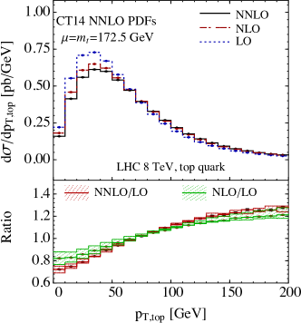
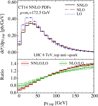
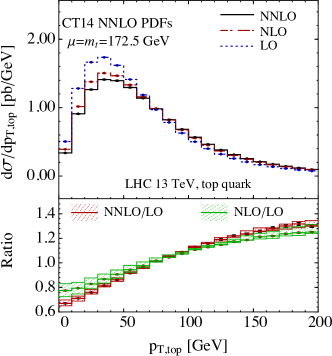
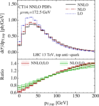
In Fig. 20 we show the transverse momentum distributions of the leading jet in top quark and anti-quark production. We adopt the anti-$k_{T}$ jet algorithm with a distance parameter of $D=0.5$. At LO these are the same as those in Fig. 19 since the top quark and jet are balanced in transverse momentum at LO. The QCD corrections show a similar strong shape dependence as the ones in Fig. 19 but are smaller in general.

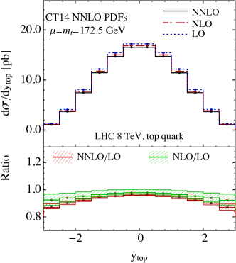
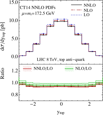
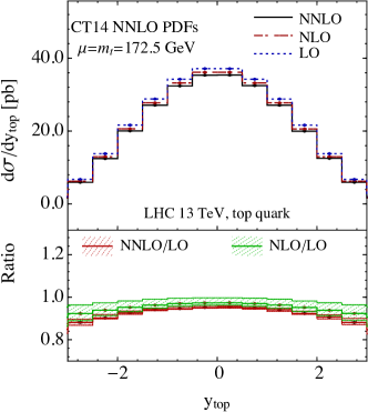
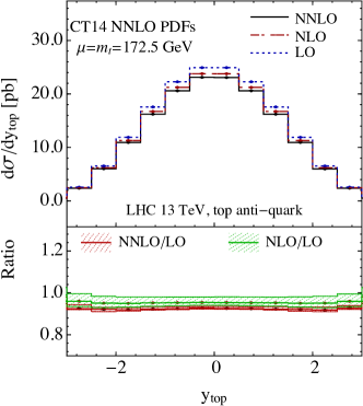
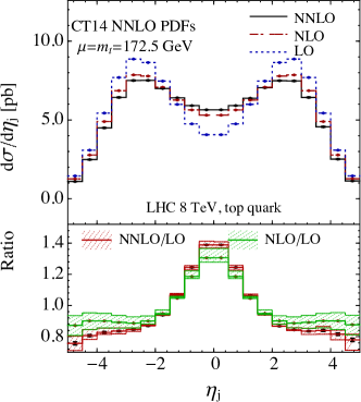
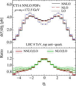
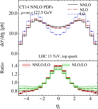
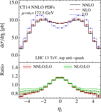
Figures 21 and 22 show the rapidity distributions of the top quark and anti-quark, and the pseudo-rapidity distributions of the leading jet in top quark and anti-quark production, respectively. The QCD corrections have only a mild effect on the rapidity distributions. The NNLO corrections are moderate and at most 6%. The scale variations at NNLO are almost contained within the NLO variation bands and are much smaller. On the hand, the QCD corrections distort the shapes of the pseudo-rapidity distributions of the leading jet with respect to LO. They fill in the cross sections in the central region and decrease them in the forward region. The NNLO corrections can be more than 10%. In the central region of pseudo-rapidity of the leading jet the QCD corrections are more pronounced for a top quark than for an anti-quark. The scale variations are greatly reduced in all cases.

Figure 20: Predicted transverse momentum distribution of the leading-jet from $t$-channel single top-quark production at 8 and 13 TeV.

Figure 21: Predicted rapidity distribution of the top (anti-)quark from $t$-channel single top-quark production at 8 and 13 TeV.

Figure 22: Predicted pseudorapidity distribution of the leading-jet from $t$-channel single top-quark production at the LHC 8 and 13 TeV.

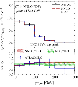
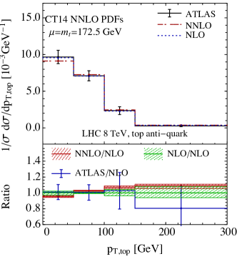
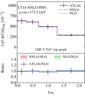
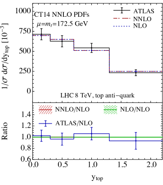
Measurements are available of parton-level differential distributions for $t$-channel single top-quark production at 8 TeV from the ATLAS collaboration with a total luminosity of 20.2 ${\rm fb^{-1}}$ 1702.02859 . We compare our theoretical predictions based on CT14 NNLO PDFs with the ATLAS measurements of the transverse momentum and rapidity distributions in Figs. 23 and 24. We choose to compare with the normalized experimental distributions for which the theoretical predictions are less sensitive to the PDFs. Ratios of predictions to the central values of the NLO prediction are shown in lower panels of all the plots. The error bars in these plots represent the total experimental uncertainties. The hatched bands show the scale variations. The transverse momentum distributions presented in Fig. 23 indicate better agreement of the NNLO predictions with the central values of the ATLAS data compared to the NLO predictions. The last bin is the only exception, but the experimental uncertainties are large. Scale variations at NNLO are negligible compared to the experimental uncertainties. As noted earlier the QCD corrections have rather small effects on the rapidity distributions of the top (anti-)quark. The lower panels of Fig, 24 show good agreement of both the NLO and NNLO predictions with the ATLAS data.

We should remark that the measured parton level distributions rely on an unfolding procedure, which depends on Monte Carlo (MC) event generators at NLO matched with parton showering 1207.5391 . A more consistent comparison of the NNLO predictions with the data should be made with unfolded measurements based on the NNLO acceptance, even if the current experimental uncertainties may already take into account part of the bias introduced by the NLO unfolding procedure.

Figure 23: Predicted transverse momentum distribution of the top (anti-)quark from $t$-channel single top-quark production at 8 TeV compared with the ATLAS data.

Figure 24: Predicted rapidity distribution of the top (anti-)quark from $t$-channel single top-quark production at 8 TeV compared with the ATLAS data.

4 Fiducial cross section

The fully differential nature of our calculation permits the computation of cross sections in a fiducial volume that matches closely the kinematic region of an experimental analysis. Such comparisons are potentially less subject to extrapolation uncertainties. Experimental measurements of fiducial cross sections show a much weaker dependence on MC event generators and thus suffer less from the related systematics. For calculations of the fiducial cross sections we assume the top quark decays 100% to $bW^{+}$ and set the $W$ boson leptonic decay branching ratio to 0.1086 for one lepton family. We use a slightly different top quark mass of 173.3 GeV here.

We define the following fiducial phase space for the LHC at 13 TeV. We use the anti-$k_{T}$ jet algorithm 0802.1189 with a distance parameter $D=0.5$. Jets are required to have transverse momentum $p_{T}>40$ GeV and pseudorapidity $|\eta|<5$. Following the CMS and ATLAS analyses, we require exactly two jets in the final state, meaning that events with additional jets are vetoed, and we require at least one of these to be a $b$-jet with $|\eta|<2.4$ CMS:2015jca . We demand the charged lepton to have a $p_{T}$ greater than 30 GeV and rapidity $|\eta|<2.4$. For the fiducial cross sections reported below we include top-quark decay to only one family of leptons. Some of the numerical results shown in this section are also reported in our earlier publication Berger:2016oht .

4.1 Total rate in the fiducial volume

fiducial [pb]		LO	NLO	NNLO
$t$ quark	total	$4.07_{-9.8\%}^{+7.6\%}$	$2.95_{-2.2\%}^{+4.1\%}$	$2.70_{-0.7\%}^{+1.2\%}$
	corr. in pro.		-0.79	-0.24
	corr. in dec.		-0.33	-0.13
$\bar{t}$ quark	total	$2.45_{-10\%}^{+7.8\%}$	$1.78_{-2.0\%}^{+3.9\%}$	$1.62_{-0.8\%}^{+1.2\%}$
	corr. in pro.		-0.46	-0.15
	corr. in dec.		-0.21	-0.08

Table 2: Fiducial cross sections for top (anti-)quark production with decay at 13 TeV at various orders in QCD with a central scale choice of $m_{t}$ in both production and decay. The scale uncertainties correspond to a quadratic sum of variations from scales in production and decay, and are shown in percentages. Corrections from purely production and purely decay are also shown.

Table 2 shows our predictions of the fiducial cross sections at different perturbative orders, with scale variations shown in percentages. We vary the renormalization and factorization scales $\mu_{R}=\mu_{F}$ in the top-quark production stage, and the renormalization scale in the decay stage, independently by a factor of two around the nominal scale choice. The resulting scale variations are added in quadrature to obtain the numbers shown in Table 2. We also show the QCD corrections from production and decay separately as defined in Eq. (2.1). All results shown in Table 2 pertain to the central scale choice $m_{t}$, as for the inclusive cross sections. The NNLO corrections from the product of $\mathcal{O}(\alpha_{\scriptscriptstyle S})$ production and $\mathcal{O}(\alpha_{\scriptscriptstyle S})$ decay can be derived by subtracting the above two contributions from the full NNLO corrections.

The NLO correction amounts to a decrease of the fiducial cross section by almost 30% for top quark production. A change this large requires investigation of the NNLO QCD corrections to examine convergence of the series. The numbers in the Table indicate that the full NNLO correction drops the fiducial cross section by another 8.5% relative to the NLO value. The corrections from decay are half of the corrections from production in general. The NNLO corrections from products of production and decay are similar in size to those from decay, but with different sign. The scale variations have been reduced by a factor of about 3 to $\sim 1\%$ at NNLO. However, for fiducial cross sections, the error bands from LO, NLO, and NNLO do not overlap each other suggesting that scale variations underestimate the true perturbative uncertainties in this case. The size of QCD corrections are similar for top anti-quark production. The ratio of fiducial cross sections for top quark and anti-quark production are 1.661, 1.657, and 1.667 at LO, NLO, and NNLO, respectively. Therefore these charge ratio observables are stable against QCD corrections even in the fiducial phase space.

In experimental analyses, the total inclusive cross sections are usually determined through extrapolation of the fiducial cross sections based on acceptance estimates obtained from MC simulations. We can use the numbers shown in Tables 1 and 2 to derive the parton-level acceptance at various orders. For top quark production, the acceptances are 0.0283, 0.0214, and 0.0201 at LO, NLO, and NNLO respectively. The NNLO corrections can change the acceptance by $6\%$ relative to the NLO value. This change also propagates into the measurement of the total inclusive cross section through extrapolation.

A comment here is appropriate on the size of QCD corrections and the choice of the QCD hard scale. With fiducial cuts applied, the jet veto introduces another hard scattering scale of $p_{T,veto}=40$ GeV in addition to $m_{t}$. A QCD scale choice $(p_{T,veto}m_{t})^{1/2}\sim m_{t}/2$ may therefore be appropriate, especially at lower perturbative orders where the gluon splitting contributions are absorbed into the bottom-quark PDF. Alternative results with a central scale choice of $m_{t}/2$ in production, with the central scale $m_{t}$ retained in decay, show better convergence of the series, although the NNLO predictions are almost unchanged. It would be worthwhile to resum the logarithmic contributions related to the scales $p_{T,veto}$ and $m_{t}$.

4.2 Distributions within the fiducial region

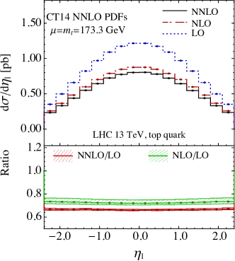
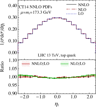
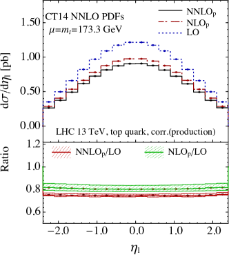
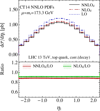
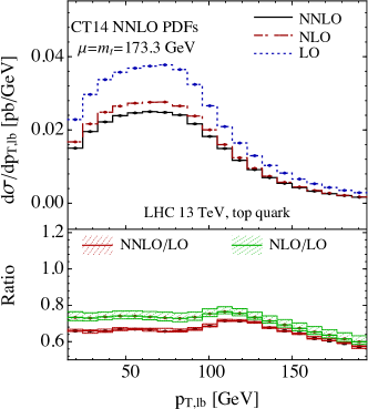
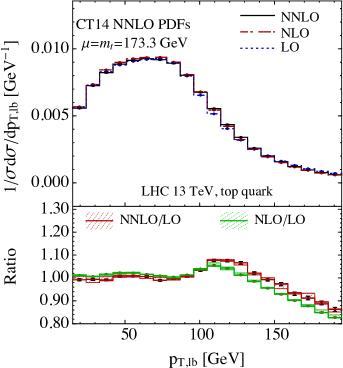
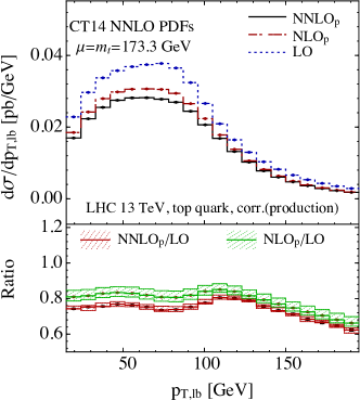
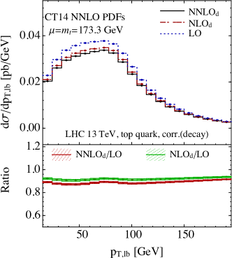
Predicted kinematic distributions within the fiducial volume can be used to compare directly with measurements without unfolding procedures. In Fig. 25 we plot the pseudo-rapidity distribution of the charged lepton, without and with normalization to the total rate for top quark production. The QCD corrections are almost constant over the full range for the unnormalized distribution. The NNLO corrections are about -6% and reduce the scale variations significantly. We observe the large gaps between the NLO and NNLO error bands. For the normalized distributions the QCD corrections are small and within 1% in general. In the lower panel of the plot on the normalized distribution, the NNLO results show MC integration fluctuations at the level of a few per mil, also shown by the error bars. In Fig. 26 we show results for the same unnormalized distribution but with QCD corrections only from the production or from the decay. Both corrections show little dependence on the pseudo-rapidity, just as for the full corrections. The size of the corrections from decay are about one-half those from production.

Figure 25: Predicted pseudo-rapidity distribution of the charged lepton from $t$-channel single top-quark production and decay at 13 TeV after fiducial cuts, including full corrections, with and without normalization respectively.

Figure 26: Predicted pseudo-rapidity distribution of the charged lepton from $t$-channel single top-quark production and decay at 13 TeV after fiducial cuts, including corrections from production and decay, respectively.

In Figs. 27 and 28 we show similar results for the transverse momentum distribution of the system composed of the charged lepton and $b$-jet. The QCD corrections from decay do not change the shape of the distribution. The size of the corrections from production tend to be enhanced in the tail region. The QCD corrections induce a nontrivial change in the shape of the normalized distribution, as can be seen from the plot of the right side of Fig. 27. The NNLO corrections can reach 5% in the tail region.

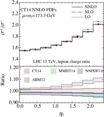
In the plot on the left of Fig. 29 we show the predicted lepton charge ratio as a function of the pseudo-rapidity. It is sensitive to the ratio $u/d$ of PDFs at different momentum fractions. Predictions at different orders in the upper panel are all based on the CT14 NNLO PDFs. The ratio increases with the pseudo-rapidity because the $u$-valence PDF is harder, extending into the region of higher $x$ than the $d$ valence PDF, where the sea-quark contributions are also smaller. The QCD corrections are small in general. The NNLO corrections are within 1% over the entire kinematic range. There are four hatched bands in the lower panel representing the spread of the LO predictions from CT14 Dulat:2015mca , MMHT2014 Harland-Lang:2014zoa , NNPDF3.0 Ball:2014uwa , and ABM12 Alekhin:2013nda PDFs with individual $1\,\sigma$ PDF uncertainties. Similar to the inclusive charge ratio shown previously, the dependence of the ratio on PDFs is much larger than the size of QCD corrections. These results indicate that sufficiently precise experimental measurements of the lepton charge ratio will further constrain the PDFs without much effect from perturbative uncertainties.

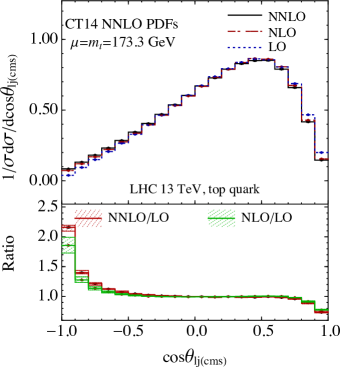
In the plot on the right side of Fig. 29 we show a normalized angular distribution in top quark production. The angle $\theta$ is defined in the reconstructed top quark rest frame between the charged lepton and the non-$b$ jet. This type of distribution is used typically for measurements of the top-quark polarization. At LO the top quark is produced highly polarized along direction of the spectator quark. Ideally one should see almost a straight line from 0 to 1 as $\cos\theta$ is varied from $-1$ to $+1$. Acceptance affects the distribution in the forward region since the charged lepton tends to be soft there. The QCD corrections can be large at both forward and backward angles, as can be seen in the lower panel. The conventional forward-backward asymmetry of the angular distribution is proportional to the top-quark polarization. The predictions are 0.383, 0.362, and 0.346 at LO, NLO, and NNLO, respectively. Thus the NNLO correction is about -4% on the forward-backward asymmetry.

Figure 27: Predicted transverse momentum distribution of the charged lepton and $b$-jet system from $t$-channel single top-quark production at 13 TeV after fiducial cuts, with full corrections included, with and without normalization respectively.

Figure 28: Predicted transverse momentum distribution of the charged lepton and $b$-jet system from $t$-channel single top-quark production at 13 TeV after fiducial cuts, including corrections from production and decay respectively.

Figure 29: Predicted lepton charge ratio as a function of the pseudo-rapidity (left plot), and normalized angular distribution between the charged lepton and the non-$b$ jet in the rest frame of the top quark (right plot), from $t$-channel single top-quark production at 13 TeV after fiducial cuts, including full corrections.

5 Summary

We presented a detailed phenomenological study of the next-to-next-to-leading order QCD corrections for $t$-channel single top (anti-)quark production including its semi-leptonic decay at the LHC. The calculations are carried out under the on-shell top-quark and the structure-function approximations, allowing the QCD corrections to be factored into three simpler pieces. The neglected corrections are suppressed either by the width of the top quark or by a color factor of $1/N_{c}^{2}$.

The NNLO corrections are generally about $-3\%$ for the total inclusive rates at LHC with different center of mass energies. The NNLO corrections can be much larger for differential distributions. They can reach a level of $10\%$ or more in certain regions of the transverse momentum distributions of the top (anti-)quark and the pseudo-rapidity distributions of the leading jet. In all cases the scale variations are greatly reduced by the NNLO corrections. We also show a comparison of the normalized parton-level distributions to the recent data from the ATLAS 8 TeV measurement. The NNLO corrections tend to move theoretical predictions closer to the measured transverse momentum distribution of the top (anti)-quark, though the reported 8 TeV data still have large uncertainties.

After top quark decay is included, we calculate and present cross sections in a restricted fiducial volume at 13 TeV, approximating experimental selections. The QCD corrections are more pronounced in this case. The NNLO corrections are about $-6\%$ for the total rate and similarly for the kinematic distributions in the fiducial volume. The corrections from pure decay are generally half the size of corrections from pure production. For normalized distributions the QCD corrections are small in general. Our predictions of the lepton charge ratio are stable against QCD corrections. Experimental measurements of this ratio can potentially provide further constraints on the ratio of the $u/d$ parton distributions in the proton. Lastly we point out that the NNLO QCD corrections can induce about $6\%$ shift on the acceptance defined as ratio of fiducial to inclusive cross sections. They may have effects of a similar level for the unfolded inclusive cross sections in experimental measurements, which are used for extraction of the electroweak coupling strength. Further studies are required to refine the exact effects of the NNLO QCD corrections on the acceptance used in experimental analyses. These can include a detailed comparison of the NNLO QCD predictions with the NLO predictions matched with parton showering, or even a possible match of the NNLO predictions with parton showering. Phenomenologcal studies such as these and detailed comparisons with data are left for future work.