Dynamical Tides in Highly Eccentric Binaries: Chaos, Dissipation and Quasi-Steady State

Abstract

Highly eccentric binary systems appear in many astrophysical contexts, ranging from tidal capture in dense star clusters, precursors of stellar disruption by massive black holes, to high-eccentricity migration of giant planets. In a highly eccentric binary, the tidal potential of one body can excite oscillatory modes in the other during a pericentre passage, resulting in energy exchange between the modes and the binary orbit. These modes exhibit one of three behaviours over multiple passages: low-amplitude oscillations, large amplitude oscillations corresponding to a resonance between the orbital frequency and the mode frequency, and chaotic growth, with the mode energy reaching a level comparable to the orbital binding energy. We study these phenomena with an iterative map that includes mode dissipation, fully exploring how the mode evolution depends on the orbital and mode properties of the system. The dissipation of mode energy drives the system toward a quasi-steady state, with gradual orbital decay punctuated by resonances. We quantify the quasi-steady state and the long-term evolution of the system. A newly captured star around a black hole can experience significant orbital decay and heating due to the chaotic growth of the mode amplitude and dissipation. A giant planet pushed into a high-eccentricity orbit may experience a similar effect and become a hot or warm Jupiter.

1 Introduction

Highly eccentric binaries appear in a variety of astrophysical contexts. In dense stellar clusters, two stars can be captured into a bound orbit with each other if a close encounter transfers enough energy into stellar oscillations (Fabian et al., 1975; Press & Teukolsky, 1977; Lee & Ostriker, 1986). Such tidally captured binaries are highly eccentric and often involve compact objects (black holes and neutron stars). Massive black holes in nuclear star clusters may tidally capture normal stars, and could build up significant masses through successive captures (Stone et al., 2017). Indeed, stars on highly eccentric orbits around massive black holes could be precursors of tidal disruption events (Rees, 1988), dozens of which have already been observed, e.g. Stone & Metzger (2016); Guillochon (2016). Heating from tidal dissipation may affect the structure of stars moving toward disruption and potentially alter the observational signal of these events (Vick et al., 2017; MacLeod et al., 2014). In exoplanetary systems, hot and warm Jupiters may be formed through high-eccentricity migration, in which a giant planet is pushed into a highly eccentric orbit by the gravitational perturbation from a distant companion (a star or planet); at periastron, tidal dissipation in the planet reduces the orbital energy, leading to inward migration and circularization of the planet’s orbit (Wu & Murray, 2003; Fabrycky & Tremaine, 2007; Nagasawa et al., 2008; Petrovich, 2015; Anderson et al., 2016; Muñoz et al., 2016). Finally, the Kepler spacecraft has revealed a class of high-eccentricity stellar binaries with short orbital periods, whose light curves are shaped by tidal distortion and reflection at periastron (Thompson et al., 2012; Beck et al., 2014; Kirk et al., 2016); many of these “heartbeat stars” also exhibit signatures of tidally induced stellar oscillations (Welsh et al., 2011; Fuller & Lai, 2012; Burkart et al., 2012; Fuller, 2017).

In a highly eccentric binary, dynamical tidal interaction occurs mainly near pericentre and manifests as repeated tidal excitations of stellar oscillation modes. Since tidal excitation depends on the oscillation phase, the magnitude and direction of the energy transfer between the orbit and the modes may vary from one pericentre passage to the next (Kochanek, 1992). Earlier works in the context of tidal-capture binaries have shown that for some combinations of orbital parameters, the energy in stellar modes may behave chaotically and grow to very large values. Mardling (1995a, b) first uncovered this phenomenon in numerical integrations of forced stellar oscillations and orbital evolution and explored the conditions for chaotic behaviour via Lyapunov analysis. In a later work, Mardling & Aarseth (2001) presented an empirical fitting formula for the location of a “chaos boundary," beyond which tighter and more eccentric binaries exhibit chaotic orbital evolution. The possibility of chaotic growth of mode energy was also explored analytically in Ivanov & Papaloizou (2004, 2007, 2011) in the context of giant planets on eccentric orbits. On the other hand, it is also expected that the long-term evolution of the binary depends on how effectively the binary components can dissipate energy (Kumar & Goodman, 1996). Indeed, in the presence of dissipation, the system may reach a quasi-steady state in which the orbit-averaged mode energy remains constant (Lai, 1996, 1997; Fuller & Lai, 2012). Numerical results from Mardling (1995b) have shown that chaotically evolving systems will eventually settle into a quiescent state of orbital evolution when modes are allowed to dissipate. The properties of this quasi-steady state that emerges from a chaotic dynamical system are unclear.

Given the important role played by dynamical tides in various eccentric stellar/planetary binary systems, a clear understanding of the dynamics of repeated tidal excitations of oscillation modes and the related tidal dissipation is desirable. In this paper, we develop an iterative map (Section 2) that accurately captures the dynamics and dissipation of the coupled “eccentric orbit + oscillation modes” system. Using this map, we aim to (i) characterize the classes of behaviours exhibited by eccentric binaries due to dynamical tides, (ii) explore the orbital parameters that lead to these behaviours, and (iii) study how the inclusion of mode damping affects the evolution of the system. As we shall see, the coupled “eccentric orbit + oscillation modes" system exhibits a richer sets of behaviours (see Section 3) than recognized in the previous works by Mardling (1995a, b) and Ivanov & Papaloizou (2004). In particular, the regime of chaotic mode growth (assuming a single mode) is determined by two dimensionless parameters (see Fig. 1 below), not one. Resonances between the oscillation mode and orbital motion can significantly influence the chaotic boundary for mode growth. In the presence of mode dissipation, we show that even a chaotic system eventually reaches a quasi-steady state (Section 4); we quantify the properties of the quasi-steady state and the long-term evolution of the system. In Section 5, we generalize our analysis to multi-mode systems.

The results of this study are applicable to a variety of systems mentioned at the beginning of this section. Some of these applications are briefly discussed in Section 6. Of particular interest is the possibility that, in the high-eccentricity migration scenario of hot Jupiter formation, chaotic mode growth, combined with non-linear damping, may lead to efficient formation of warm Jupiters and hot Jupiters.

2 Iterative Map for Mode Amplitudes

Consider a binary system consisting of a primary body $M$ (a star or planet) on an eccentric orbit with a companion $M^{\prime}$ (treated as a point mass). Near pericentre, the tidal force from $M^{\prime}$ excites oscillations in $M$. When the oscillation amplitudes are sufficiently small, we can follow the evolution of the modes and the orbit using linear hydrodynamics. For highly eccentric orbits ($1-e\ll 1$), the orbital trajectory around the pericentre remains almost unchanged even for large changes in the binary semi-major axis. Under these conditions, the full hydrodynamical solution of the system can be reduced to an iterative map (see Appendix A). We present the following map for a single-mode system and will discuss later the effects of multiple modes.

We define the dimensionless mode energy and binary orbital energy in units of $|E_{B,0}|$ (the initial binary orbital energy), i.e., ${\tilde{E}}=E/|E_{B,0}|$. Consider a single mode of the star with frequency $\omega$ and (linear) damping rate $\gamma$. Let $a_{k-1}$ be the mode amplitude just before the $k$-th pericentre passage. Immediately after the $k$-th passage, the mode amplitude becomes

$$a_{k-}=a_{k-1}+\Delta a,$$ (1)

where $\Delta a$ (real) is the mode amplitude change in the “first” passage (i.e., when there is no pre-existing oscillation). We normalize $a_{k}$ such that the (dimensionless) mode energy just after $k$-th passage is ${\tilde{E}}_{k-}=|a_{k-}|^{2}$. Thus the energy transfer to the mode in the $k$-th passage is

$$\Delta{\tilde{E}}_{k} =|a_{k-}|^{2}-|a_{k-1}|^{2}=|a_{k-1}+\Delta a|^{2}-|a_{k-1}|^{2}.$$ (2)

In physical units, the energy transfer in the “first" passage is given by $\Delta E_{1}=(\Delta a)^{2}|E_{B,0}|$. The binary orbital energy (${\tilde{E}}_{B,k}$) immediately after the $k$-th passage is given by

$${\tilde{E}}_{B,k}={\tilde{E}}_{B,k-1}-\Delta{\tilde{E}}_{k}={\tilde{E}}_{B,0}-\sum_{j=1}^{k}\Delta{\tilde{E}}_{j},$$ (3)

and the corresponding orbital period is

$${P_{k}\over P_{0}}=\left({{\tilde{E}}_{B,0}\over{\tilde{E}}_{B,k}}\right)^{3/2},$$ (4)

where ${\tilde{E}}_{B,0}=-1$. The mode amplitude just before the $(k+1)$-th passage is

$$a_{k}=a_{k-}\,\text{e}^{-(\text{i}\omega+\gamma)P_{k}}=\left(a_{k-1}+\Delta a\right)\,\text{e}^{-(\text{i}+\hat{\gamma}){\hat{P}}_{k}},$$ (5)

where we have defined the dimensionless damping rate and orbital period

$${\hat{\gamma}}={\gamma\over\omega},\quad{\hat{P}}_{k}=\omega P_{k}.$$ (6)

Equations (1)-(5) complete the map from one orbit to the next, starting from the initial condition $a_{0}=0$, ${\tilde{E}}_{0}=0$, ${\tilde{E}}_{B,0}=-1$. In the absence of dissipation, this map reduces to that of Ivanov & Papaloizou (2004). The map depends on three parameters:

$${\hat{P}}_{0} \equiv\omega P_{0},$$ (7)

$$|\Delta{\hat{P}}_{1}| \equiv\omega|\Delta P_{1}|\simeq{3\over 2}{\hat{P}}_{0}(\Delta a)^{2}=\frac{3}{2}{\hat{P}}_{0}\left(\frac{\Delta E_{1}}{|E_{B,0}|}\right),$$ (8)

$${\hat{\gamma}} ={\gamma\over\omega}={\gamma P_{0}\over{\hat{P}}_{0}}={1\over{\hat{P}}_{0}}\left({P_{0}\over t_{\rm damp}}\right).$$ (9)

To relate ${\hat{P}}_{0}$ and $|\Delta{\hat{P}}_{1}|$ to the physical parameters of the system, we scale the mode frequency $\omega$ to $\Omega_{\rm{peri}}\equiv(GM_{t}/r_{\rm{peri}}^{3})^{1/2}$ (where $M_{t}=M+M^{\prime}$, and $r_{\rm{peri}}$ is the pericentre distance), and find

$${\hat{P}}_{0}=\frac{2\pi(\omega/\Omega_{\rm{peri}})}{(1-e)^{3/2}}.$$ (10)

The parameter $|\Delta{\hat{P}}_{1}|$ is related to the energy transfer in the “first” pericentre passage via $|\Delta{\hat{P}}_{1}|/{\hat{P}}_{0}=(3/2)|\Delta E_{1}/E_{B,0}|$. If we scale $r_{\rm{peri}}$ by the tidal radius $r_{\rm tide}=R(M_{t}/M)^{1/3}$ (where $R$ is the stellar radius), i.e., $\eta=r_{\rm{peri}}/r_{\rm tide}$, we have, for $l=2$,

$$\Delta E_{1}=-{G{M^{\prime}}^{2}R^{5}\over r_{\rm{peri}}^{6}}\,T(\eta,\omega/\Omega_{\rm{peri}},e),$$ (11)

where $T$ is a dimensionless function of $\eta,$ $\omega/\Omega_{\rm{peri}},$ and $e$ (though $T$ becomes independent of $e$ as $e$ approaches unity). The exact form of $T(\eta,\omega/\Omega_{\rm{peri}},e)$ is provided in Appendix A. Then,

$$|\Delta{\hat{P}}_{1}|={6\pi(\omega/\Omega_{\rm{peri}})\over(1-e)^{5/2}}\left({M^{\prime}\over M}\right)\left({M\over M_{t}}\right)^{\!5/3}\eta^{-5}T(\eta,\omega/\Omega_{\rm{peri}},e).$$ (12)

In general, $|\Delta{\hat{P}}_{1}|$ falls off steeply with $\eta$. However, even when $\eta$ is large (weak tidal encounter), $|\Delta{\hat{P}}_{1}|$ can be significant for highly eccentric systems (with $1-e\ll 1$).

The map (1)-(5) assumes that (i) energy transfer occurs instantaneously at pericentre; (ii) at each pericentre passage, the change in mode amplitude, $a_{k-}-a_{k-1}$, is the same; and (iii) the mode energy is always much less than the binding energy of the star. The first condition is satisfied when $1-e\ll 1$. Eccentric systems that exhibit oscillatory behaviour (see Section 3) easily satisfy this condition over many orbits. Chaotic systems (see Section 3) can evolve through a larger range of mode energies and orbital eccentricities. For this condition to hold throughout evolution, they must begin with very large eccentricities. The second condition requires that the pericentre distance remains constant, which in turn requires that the fractional change in orbital angular momentum, $\Delta L/L$, remain small throughout orbital evolution. Using $\Delta L\sim\Delta E_{B}/\Omega_{\rm{peri}}$ as an estimate, we find that the condition $\Delta L/L\ll 1$ becomes

$$\frac{\Delta L}{L}\sim{1\over 2\sqrt{2}}\Delta{\tilde{E}}_{B}(1-e)\ll 1.$$ (13)

Thus, for sufficiently eccentric orbits, $r_{\rm{peri}}$ is roughly constant even when the orbital energy changes by $\Delta{\tilde{E}}_{B}\sim 10$. The third condition, $E_{k}\ll GM^{2}/R$, yields the expression

$$\frac{{\tilde{E}}_{k}(1-e)}{2\eta}\left({M^{\prime}\over M}\right)\left(\frac{M_{t}}{M}\right)^{\!-1/3}\ll 1.$$ (14)

Again, this is easiest to satisfy for very eccentric orbits.

Figure 1: The maximum mode energy reached in $10^{4}$ orbits as a function of $|\Delta\hat{P}_{1}|/2\pi$ and $\hat{P}_{0}/2\pi$. The energy is normalized to the initial orbital energy of the binary. In the dark blue regions, the mode exhibits low-energy oscillations. In the light green regions, the mode exhibits high-amplitude oscillations corresponding to a resonance. The red regions indicate chaotic mode evolution.

3 Mode Energy Evolution without Dissipation

We first study the dynamics of the “eccentric orbit + mode" system without dissipation (${\hat{\gamma}}=0$). The iterative map described in equations (1)-(5) displays a variety of behaviours depending on $\hat{P}_{0}$ and $|\Delta\hat{P}_{1}|$. We can gain insight into the evolution of the system by recording $\tilde{E}_{\rm{max}}$, the maximum mode energy reached over many orbits; this quantity reveals whether energy transfer to stellar modes is relatively small or whether the orbit can change substantially by transferring large amounts of energy. Figure 1 shows $\tilde{E}_{\rm{max}}$ after $10^{4}$ orbits for systems with a range of $\hat{P}_{0}$ and $|\Delta\hat{P}_{1}|$. Similarly, Fig. 2 displays $\tilde{E}_{\rm{max}}$ as a function of $r_{\rm peri}$ and $e$ for an $n=1.5$ polytrope stellar model in a binary with mass ratio $M^{\prime}/M=1$. The relationship between the physical parameters $r_{\rm peri}$ and $e$ and the mapping parameters ${\hat{P}}_{0}$ and $|\Delta{\hat{P}}_{1}|$ is given by equations (10) and (12) (see Appendix A for more detail).

Figure 2: The maximum mode energy reached in $10^{4}$ orbits as a function of the pericentre distance, $r_{\rm peri}$, and $e$ for the $l=2$ f-mode of an $n=1.5$ polytrope in a binary with mass ratio $M^{\prime}/M=1$. The energy is normalized to the energy transferred in the first pericentre passage, $\Delta{\tilde{E}}_{1}$. In the dark blue region, the mode exhibits low-amplitude oscillations. The light blue “fingerprint" ridges correspond to resonances. The yellow/orange region displays chaotic mode evolution. The black line indicates $|\Delta{\hat{P}}_{1}|=1$. Note that, in this figure, the mode energy of the chaotic systems may not have attained the true “theoretical" maximum [see equation (26)] in $10^{4}$ orbits; the energy may continue to climb to a large value if the system is allowed to continue evolving.

The system evolution has a complex dependence on $\hat{P}_{0}$ and $|\Delta\hat{P}_{1}|$. In general, the mode energy exhibits oscillatory behaviour for small $|\Delta\hat{P}_{1}|$ and chaotic growth for large $|\Delta\hat{P}_{1}|$. However, Fig. 1 shows exceptions to this trend. The figure also suggests that the response to $\hat{P}_{0}$ is periodic and the mode amplitude is larger in magnitude near resonances where the orbital frequency is commensurate with the mode frequency. The map displays three primary types of behaviours — low-amplitude oscillation, resonant oscillation, and chaotic evolution. Transitions between the three regimes are complicated. However, within each regime, $\tilde{E}_{\rm{max}}$ exhibits simple dependence on $\hat{P}_{0}$ and $|\Delta\hat{P}_{1}|$. We now discuss the three types of behaviour in detail.

3.1 Oscillatory Behaviour

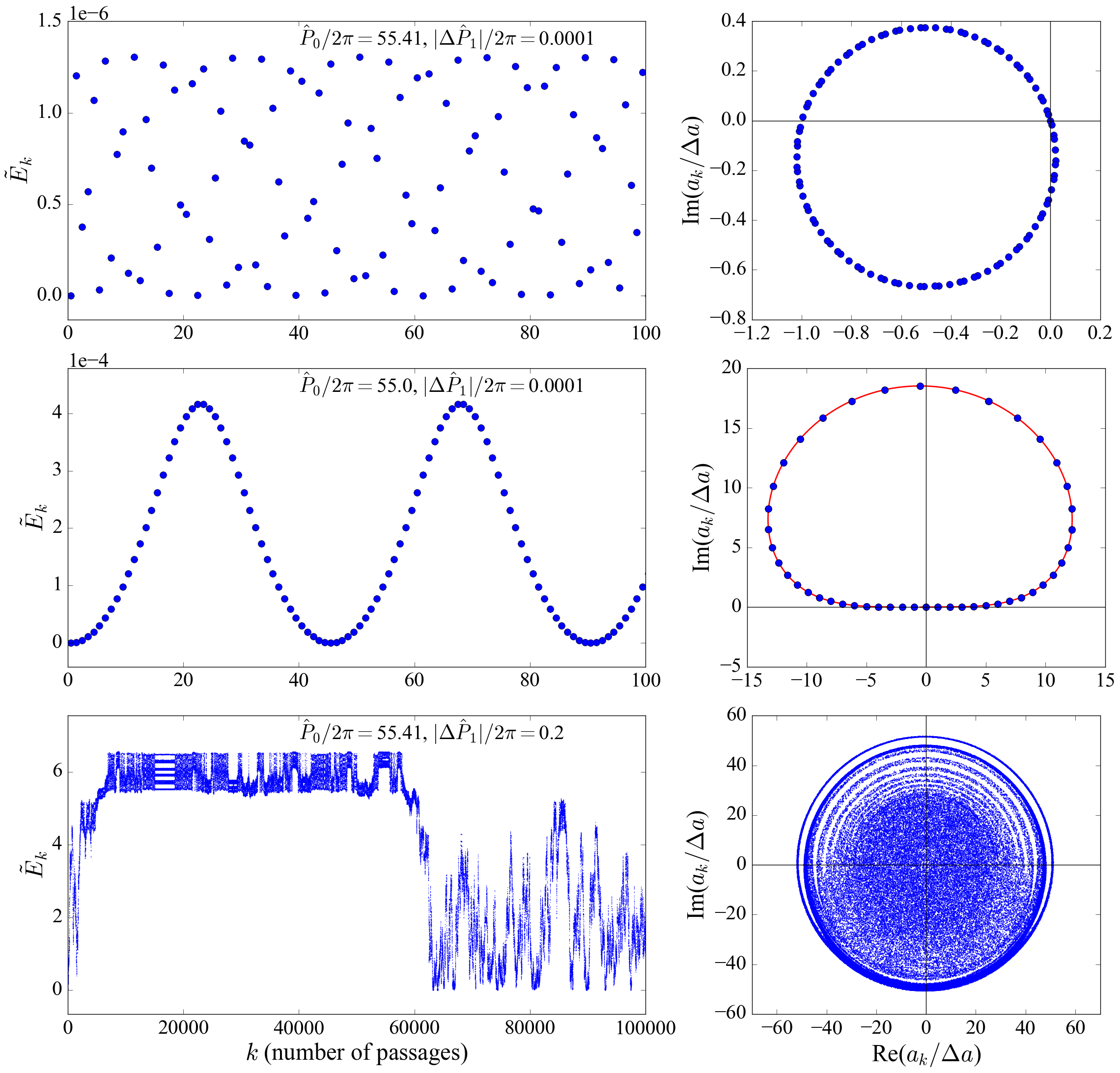
Figure 3: Left Column: The evolution of the mode energy over multiple pericentre passages. Right Column: The complex mode amplitude $a_{k}$ (normalized to $\Delta a$, the change in mode amplitude during the first pericentre passage). From top to bottom, the three rows correspond to different types of behaviours — low-amplitude oscillations, resonant behaviour, and chaotic evolution. The red line is from equation (65) in Appendix B.1.

When $|\Delta{\hat{P}}_{1}|/(2\pi)\lesssim 0.05$ and $\hat{P}_{0}/(2\pi)$ is not close to an integer, the mode exhibits low-amplitude oscillations, shown in the top panels of Fig. 3. In this regime, the orbital period is nearly constant (${\hat{P}}_{k}\simeq{\hat{P}}_{0}$), and the map from equations (1)-(5) can be written simply as

$$a_{k}\simeq(a_{k-1}+\Delta a)\,e^{-i{\hat{P}}_{0}}.$$ (15)

This can be solved with the initial condition $a_{0}=0$, yielding

$$a_{k}\simeq\frac{\Delta a}{e^{i{\hat{P}}_{0}}-1}\left(1-e^{-i{\hat{P}}_{0}k}\right).$$ (16)

Note that, in the complex plane, this solution has the form of a circle of radius $|1/(e^{i{\hat{P}}_{0}}-1)|$ centred on $1/(e^{i{\hat{P}}_{0}}-1)$, as shown in Fig. 3 [a result previously seen in Ivanov & Papaloizou (2004)]. From equation (16), the maximum mode energy in this regime is

$$\tilde{E}_{\rm{max}}\simeq\frac{2(\Delta a)^{2}}{1-\cos{{\hat{P}}_{0}}}.$$ (17)

This result demonstrates that our assumption of ${\hat{P}}_{k}\simeq{\hat{P}}_{0}$ performs well when $(\Delta a)^{2}\ll 1$ and ${\hat{P}}_{0}$ is not too close to an integer multiple of $2\pi$. Under these conditions, the mode energy remains of order $(\Delta a)^{2}=\Delta{\tilde{E}}_{1}$, the energy transfer in the “first” pericentre passage.

3.2 Resonance

Figure 1 indicates that the stellar mode exhibits large-amplitude oscillations for ${\hat{P}}_{0}\simeq 2\pi N$ (with $N=$integer), i.e., when the orbital period $P_{0}$ is nearly an integer multiple of the mode period $2\pi/\omega$. To understand this behaviour, we assume ${\tilde{E}}_{k}=|a_{k}|^{2}\ll 1$, which holds true in the non-chaotic regime. With no dissipation, equation (4) is replaced by

$${\hat{P}}_{k}\simeq{\hat{P}}_{0}\left(1-\frac{3}{2}|a_{k-}|^{2}\right)={\hat{P}}_{0}-|\Delta{\hat{P}}_{1}||z_{k}|^{2},$$ (18)

where we have defined $z_{k}\equiv a_{k-}/\Delta a$ and used equation (8). The map can then be written as

$$z_{k+1}=1+z_{k}\,e^{-i{\hat{P}}_{k}}\simeq 1+z_{k}\,e^{-i{\hat{P}}_{0}+i|\Delta{\hat{P}}_{1}||z_{k}|^{2}}.$$ (19)

Near a resonance, with $|\delta{\hat{P}}_{0}|=|{\hat{P}}_{0}-2\pi N|\ll 1$, the above map can be further simplified to $z_{k+1}-z_{k}\simeq 1+z_{k}(-i\delta{\hat{P}}_{0}+i|\Delta P_{1}||z_{k}|^{2})$. The maximum mode amplitude near resonance is determined by setting the non-linear term $|\Delta{\hat{P}}_{1}||z_{k}|^{3}\sim 1$, giving $|z_{\rm{res}}|\sim|\Delta{\hat{P}}_{1}|^{-1/3}$. The corresponding mode energy is

$${\tilde{E}}_{\text{res}}\sim{(\Delta a)^{2}\over|\Delta{\hat{P}}_{1}|^{2/3}}\sim{|\Delta{\hat{P}}_{1}|^{1/3}\over{\hat{P}}_{0}}.$$ (20)

Equation (20) is valid for $|\delta{\hat{P}}_{0}|\lesssim|\Delta{\hat{P}}_{1}|^{1/3}$, and agrees with our numerical result (see Appendix B.1 for more details).

3.3 Chaotic Growth

Chaotic growth of mode energy typically occurs when $|\Delta\hat{P}_{1}|\gtrsim 1$, i.e., when enough energy is transferred in a pericentre passage to change the orbital period and cause appreciable phase shift of the mode. In this regime, the mode amplitude fills a circle in the complex plane after the binary evolves for many orbits, as shown in the bottom panels of Fig. 3.

We can verify that the dynamical behaviour of systems with a large $|\Delta{\hat{P}}_{1}|$ is chaotic by examining the difference between a trajectory and its shadow to estimate the Lyapunov exponent. The shadow trajectory is calculated with a slightly different initial value $a_{0,{\rm shadow}}$, such that $\delta a_{0}\equiv|a_{0,\text{shadow}}|-|a_{0}|\ll 1$. We follow the evolution of $\delta a_{k}\equiv||a_{k,\text{shadow}}|-|a_{k}||$. For chaotic behaviour, we expect

$$\delta a_{k}\approx\delta a_{0}\,\text{e}^{\lambda k},$$ (21)

where $\lambda$ is the Lyapunov exponent.

Figure 4 suggests that systems with $|\Delta{\hat{P}}_{1}|\sim 1$ indeed undergo chaotic evolution, with $\delta a_{k}$ growing exponentially (but eventually saturating when $\delta a_{k}\sim 0.1$). For the system depicted in Fig. 4, $\lambda\approx 1.77$. The exact value of $\lambda$ can change slightly with the parameters ${\hat{P}}_{0}$ and $|\Delta{\hat{P}}_{1}|$. Similar Lyapunov calculations were preformed in Mardling (1995a, b) to determine numerically the boundary for chaotic behaviour in the $r_{\rm peri}-e$ plane [e.g. Fig. 13 in Mardling (1995a), which qualitatively agrees with our Fig. 2]. The condition $|\Delta{\hat{P}}_{1}|\gtrsim 1$ for chaotic behaviour was first identified by Ivanov & Papaloizou (2004).

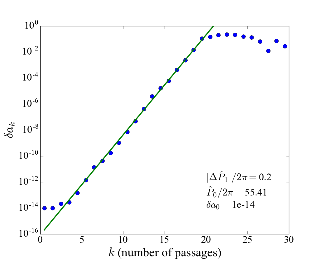
Figure 4: The blue dots show the difference between the mode amplitude of a trajectory and its shadow, $\delta a_{k}$, as a function of orbits. The green line shows a fit to the exponential rise with $\lambda\approx 1.77$, where $\lambda$ is defined in equation (21). For $k\gtrsim 20$, $\delta a_{k}$ saturates around 0.1.

While the Lyapunov saturation of $\delta a_{k}$ occurs after 10’s of orbits, the mode energy can continue to climb over much longer timescales (as in the bottom panel of Fig. 3). In the absence of dissipation, the mode amplitude map is simply

$$a_{k}=(a_{k-1}+\Delta a)\,e^{-i{\hat{P}}_{k}},\quad{\rm with}~{}~{}{\hat{P}}_{k}={\hat{P}}_{0}\left(1+|a_{k}|^{2}\right)^{-3/2}.$$ (22)

When the change in orbital period between pericentre passages, $\Delta{\hat{P}}_{k}={\hat{P}}_{k}-{\hat{P}}_{k-1}$, is much larger than unity, ${\hat{P}}_{k}$ approximately takes on random phases. This random-phase model, previously studied in Mardling (1995a); Ivanov & Papaloizou (2004), captures the key features of mode growth in the chaotic regime (see Fig. 5). The mode energy after the $k$-th passages can be written as

$$\tilde{E}_{k}=\sum_{j=1}^{k}\Delta\tilde{E}_{j}=\sum_{j=1}^{k}\left[(\Delta a)^{2}+2(\Delta a){\rm Re}(a_{j-1})\right].$$ (23)

If we assume that $a_{j-1}$ exhibits random phases, then

$$\langle\tilde{E}_{k}\rangle\sim(\Delta a)^{2}k,$$ (24)

a result previously obtained by Mardling (1995a) and Ivanov & Papaloizou (2004). This provides a crude description of the chaotic mode growth, shown in Fig. 5.

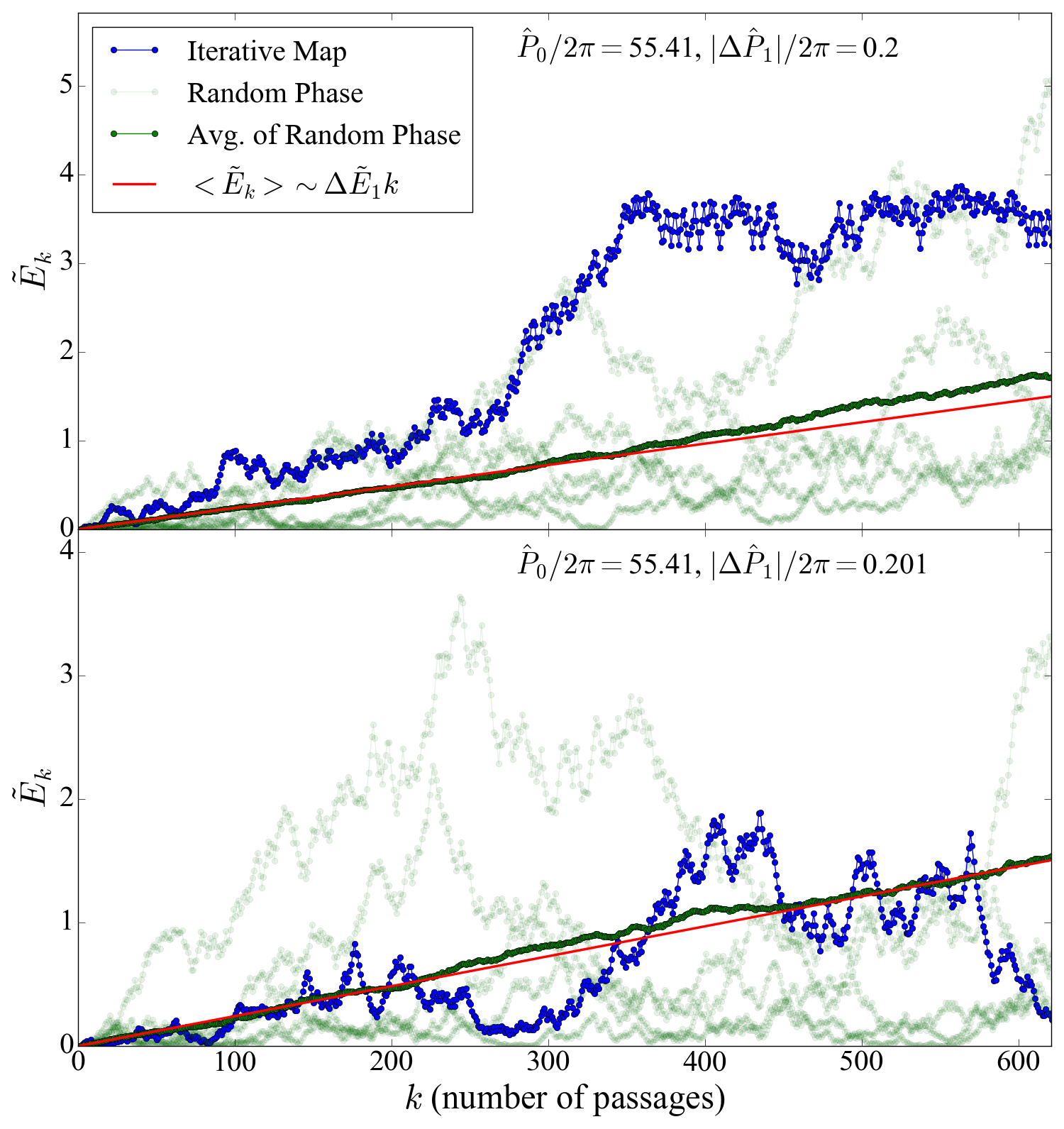
Figure 5: The mode energy evolution for two slightly different values of $|\Delta{\hat{P}}_{1}|$. The blue lines are the results from the iterative map; the light green lines show examples of the random phase model [where ${\hat{P}}_{k}$ in equation (22) takes on random values between 0 and $2\pi$]; the dark green is an average of 100 iterations of the random phase model; and the red lines show the expected average growth of the mode energy in the diffusion model.

Although $\tilde{E}_{\text{max}}$ can become very large, Fig. 3 suggests that the mode energy cannot exceed a maximum value, a feature not captured by the random-phase model, but previously seen in some examples of numerical integrations of chaotic mode evolution (Mardling, 1995b). This can be understood from the fact that as the mode energy increases, the the range of possible $\Delta{\hat{P}}_{k}$ decreases. Indeed, from equation (22) we find

$$\Delta{\hat{P}}_{k}\equiv{\hat{P}}_{k}-{\hat{P}}_{k-1}\simeq-3\Delta a{\hat{P}}_{0}\frac{{\>\rm{Re}}(a_{k-1})}{(1+|a_{k-1}|^{2})^{5/2}}.$$ (25)

Setting $\Delta{\hat{P}}_{k}\sim 1$ leads to a maximum mode energy

$$\tilde{E}_{\text{max}}=\bigl{(}|a_{k}|^{2}\bigr{)}_{\rm max}\sim({\hat{P}}_{0}\Delta a)^{1/2}\sim\left(|\Delta{\hat{P}}_{1}|{\hat{P}}_{0}\right)^{1/4}.$$ (26)

More discussion on the maximum mode energy in the chaotic regime can be found in Appendix B.3. Note that ${\tilde{E}}_{\text{max}}$ of order a few can be easily reached for a large range of ${\hat{P}}_{0}$ and $|\Delta{\hat{P}}_{1}|$ (see Fig. 3). Such a large mode energy implies order unity change in the semi-major axis of the orbit, but for $1-e\ll 1$ it does not necessarily violate the requirements needed for the validity of the iterative map [see equations (13)-(14)].

4 Mode Energy Evolution with Dissipation

We now consider the effect of dissipation on the evolution of the system. In the presence of mode damping ($\gamma\neq 0$), energy is preferentially transferred from the orbit to the stellar mode which then dissipates, causing long-term orbital decay. In the extreme case when the mode damping time $t_{\rm damp}=\gamma^{-1}$ is shorter than the orbital period $P$, the energy transfer in each pericentre passage $\Delta E_{1}$ is dissipated, and the orbital energy $E_{B}$ simply decays according to

$${dE_{B}\over dt}\simeq-{\Delta E_{1}\over P},\quad({\rm for}~{}t_{\rm damp}\lesssim P).$$ (27)

Below, we will consider the more realistic situation of $t_{\rm damp}\gg P$.

4.1 Quasi-Steady State

Consider a system with $|\Delta{\hat{P}}_{1}|\ll 1$ and an orbital period that is far from resonance. The mode energy will stay around $\Delta E_{1}$, and can attain a quasi-steady state after a few damping times (see Fig. 6). Indeed, since the orbital period $P$ remains roughly constant over multiple damping times, the map simplifies to

$$a_{k}\simeq(a_{k-1}+\Delta a)\,e^{-(i+\hat{\gamma}){\hat{P}}}.$$ (28)

Assuming $a_{0}=0$, we find

$$a_{k}\simeq\frac{\Delta a}{\text{e}^{(\text{i}+\hat{\gamma})\hat{P}}-1}\left[1-\text{e}^{-(\text{i}+\hat{\gamma})\hat{P}k}\right].$$ (29)

Clearly, the mode amplitude approaches a constant value after a few damping times ($kP\gg\gamma^{-1}$), and the mode energy reaches the steady-state value (Lai, 1997):

$$\tilde{E}_{\rm{ss}}\simeq\frac{\Delta{\tilde{E}}_{1}\,e^{-\hat{\gamma}\tilde{P}}}{2(\cosh\hat{\gamma}\hat{P}-\cos\hat{P})}\simeq\frac{\Delta{\tilde{E}}_{1}}{4\sin^{2}({\hat{P}}/2)+({\hat{\gamma}}{\hat{P}})^{2}},$$ (30)

where the second equality assumes $\hat{\gamma}{\hat{P}}=\gamma P\ll 1$, or $t_{\rm{damp}}\gg P$. The steady-state energy is of order $\Delta{\tilde{E}}_{1}$, provided that the system is not near a resonance. In the steady state, the star dissipates all the “additional” energy gained at each pericentre passage, and thus the orbital energy decays according to

$${d{\tilde{E}}_{B}\over dt}\simeq-2\gamma\tilde{E}_{\text{ss}}~{}~{}~{}{\rm or}~{}~{}~{}{dE_{B}\over dt}\simeq-{2{E}_{\text{ss}}\over t_{\rm damp}}, \quad({\rm for}~{}t_{\rm damp}\gg P).$$ (31)

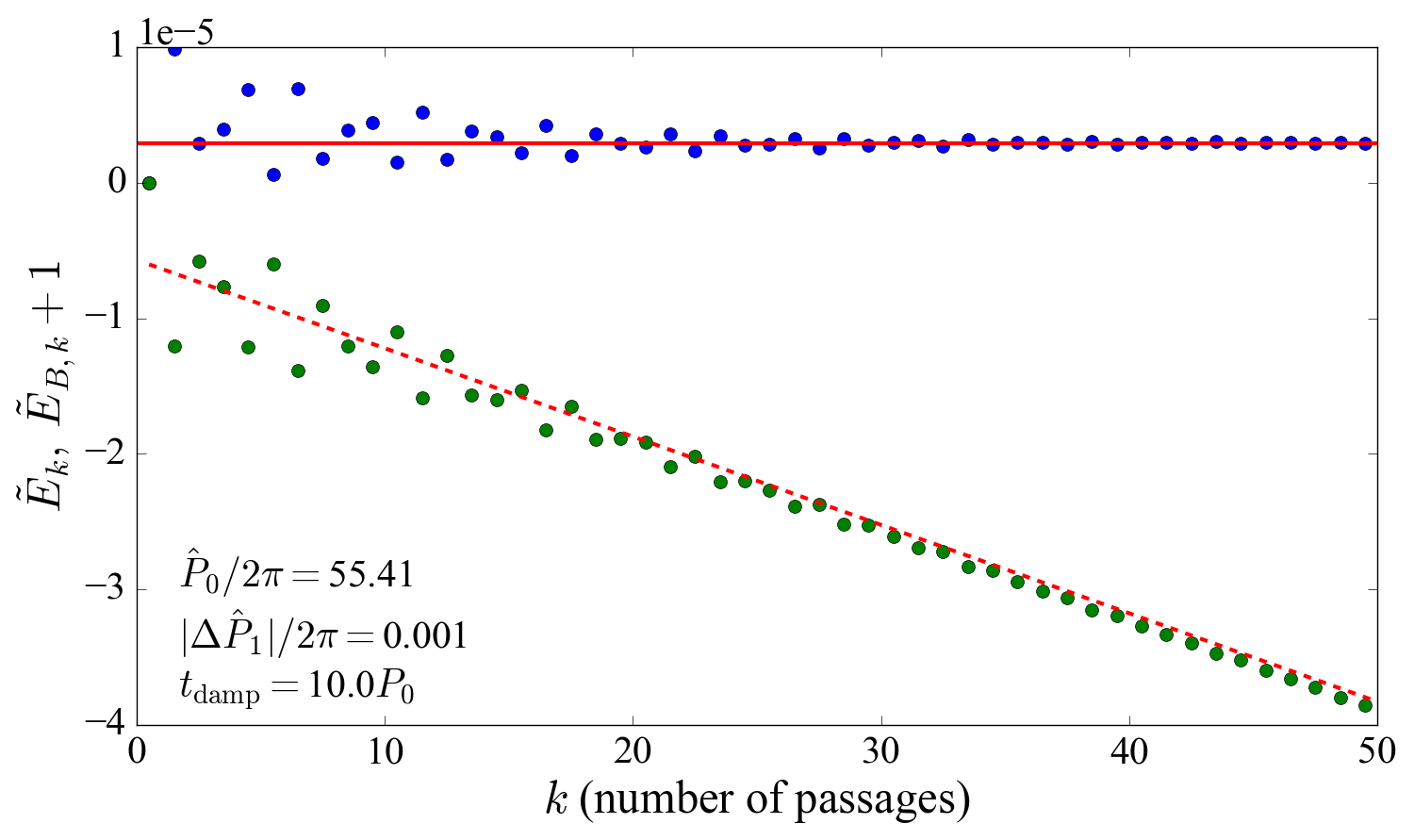
Figure 6: The stellar mode energy (blue dots) and the orbital energy (green dots; shifted for comparison) over $50$ pericentre passages. Energy is normalized to the initial orbital energy of the binary. The solid red line shows the steady-state mode energy given by equation (30), and the dashed red line shows the orbital decay rate from equation (31).

4.2 Passing Through Resonances

As the binary orbit experiences quasi-steady decay, it will encounter resonances with the stellar mode (${\hat{P}}/2\pi=$integer), during which rapid orbital decay occurs (see Fig. 7).

Figure 7: The mode energy (in blue) and the orbital energy (in green) over many pericentre passages. Energy is normalized to the initial orbital energy of the binary. The analytic orbital decay rate for the quasi-steady state is plotted in dashed red. The red lines are spaced by $5.46{\tilde{E}}_{\rm res}$ with ${\tilde{E}}_{\rm{res}}$ given by equation (20).

The change in orbital energy when a system moves through a resonance depends on how the resonance time $t_{\rm res}$ (the timescale for the mode energy of a system near resonance to reach ${\tilde{E}}_{\text{res}}$) compares with $t_{\text{damp}}$. In most likely situations, the resonance time $t_{\rm res}\sim P/|\Delta{\hat{P}}_{1}|^{1/3}$ (see Appendix B.2) is much shorter than $t_{\rm damp}$, so the orbital energy is quickly transferred to the stellar mode as the system approaches the resonance, and the mode energy reaches the maximum resonance value given by equation (20). All of this energy is dissipated within a few $t_{\rm damp}$, resulting in a net change in the orbital energy during the resonance $\Delta{\tilde{E}}_{B,{\rm res}}\simeq{\tilde{E}}_{\rm res}\sim|\Delta{\hat{P}}_{1}|^{1/3}/{\hat{P}}$. By comparison, the quasi-steady orbital energy change between adjacent resonances [from ${\hat{P}}=2\pi N$ to ${\hat{P}}=2\pi(N-1)$] is (assuming $N\gg 1$)

$$\Delta{\tilde{E}}_{B,\text{ss}}\simeq\frac{4\pi}{3{\hat{P}}}.$$ (32)

Thus $\Delta{\tilde{E}}_{B,{\rm res}}/\Delta{\tilde{E}}_{B,\text{ss}}\sim 0.2|\Delta{\hat{P}}_{1}|^{1/3}$. In practice, systems that evolve into resonance rather than starting in resonance will reach a maximum mode energy of a few times equation (20), so $\Delta{\tilde{E}}_{B,{\rm res}}$ can be comparable to $\Delta{\tilde{E}}_{B,\text{ss}}$.

4.3 Tamed Chaos

In the presence of dissipation, even systems that experience chaotic mode growth eventually settle into a quasi-steady state. Figure 8 depicts an example. We see that initially the mode energy increases rapidly, accompanied by a large decrease in the orbital energy. This behaviour has been seen in numerical integrations of forced stellar oscillations and orbital evolution by Mardling (1995b), where the orbital eccentricity quickly decreases to a value dictated by the “chaos boundary" before settling into a state of gradual decay. With our exact “dissipative" map, we can predict the steady-state mode energy and orbital decay rate that emerge after a period of chaotic evolution. For systems with relatively large damping rates, the mode energy may not reach the full “chaotic maximum” given by equation (26). However, for systems with relatively small damping rates, the full maximum energy is attainable. In either case, the mode energy ultimately decays to a quasi-steady value of order $\Delta E_{1}$ after a timescale of $\sim t_{\rm damp}\ln(E_{\rm max}/\Delta E_{1})$. The evolution of the system in quasi-steady state is well described by equations (30)-(31).

We can understand how an initially chaotic system (with $|\Delta{\hat{P}}_{1}|\sim 1$) is brought into the “regular” regime by renormalizing various quantities to their “post-chaotic” values (see the lower panel of Fig. 8). Recall that the key parameter that determines the dynamical state of the system is $|\Delta{\hat{P}}|=\omega|\Delta P|$, with $\Delta P$ the change in the orbital period in a the first pericentre passage (i.e. when there is no prior oscillation). Since $|\Delta P|/P\simeq 3\Delta E/(2|E_{B}|)$ and $\Delta E$ is independent of the semi-major axis $a$ (it depends only $r_{\rm{peri}}$, which is almost unchanged), we find $|\Delta{\hat{P}}|\propto a^{5/2}\propto(1-e)^{-5/2}$ [for $r_{\rm{peri}}=$ constant; see equation (12)]. Thus, after significant orbital decay (with $a$ decreased by a factor of a few), $|\Delta{\hat{P}}|$ is reduced to a “non-chaotic” value, and the system settles into the regular quasi-steady state.

We can approximate the orbital parameters of a “tamed" chaotic system that has reached quasi-steady state from the evolution of the orbital energy, ${\tilde{E}}_{\rm B}$. Our map assumes that angular momentum is conserved as the orbit evolves. Given this constraint, the orbital eccentricity just before the $(k+1)$-th pericentre passage is

$$e_{k}=\left[1-|{\tilde{E}}_{B,k}|(1-e_{0}^{2})\right]^{1/2}.$$ (33)

As an example, a system with initial eccentricity $e_{0}=0.99$ that settles to a quasi-steady state orbital energy ${\tilde{E}}_{\rm B}\approx-5$ would retain an eccentricity of $e\approx 0.95$. Note that less eccentric binaries (even $e=0.9$) can circularize substantially over the course of chaotic evolution and strain the assumptions of our map (see Section 2).

Our model assumes linear mode damping. In reality, modes that are excited to high amplitudes may experience non-linear damping. This will likely make the system evolve to the quasi-steady state more quickly. Other than this change of timescale, we expect that the various dynamical features revealed in our model remain valid. We note that a rapidly heated star/planet may undergo significant structural change depending on where heat is deposited. This may alter the frequencies of stellar modes. Our current model does not account for such feedback.

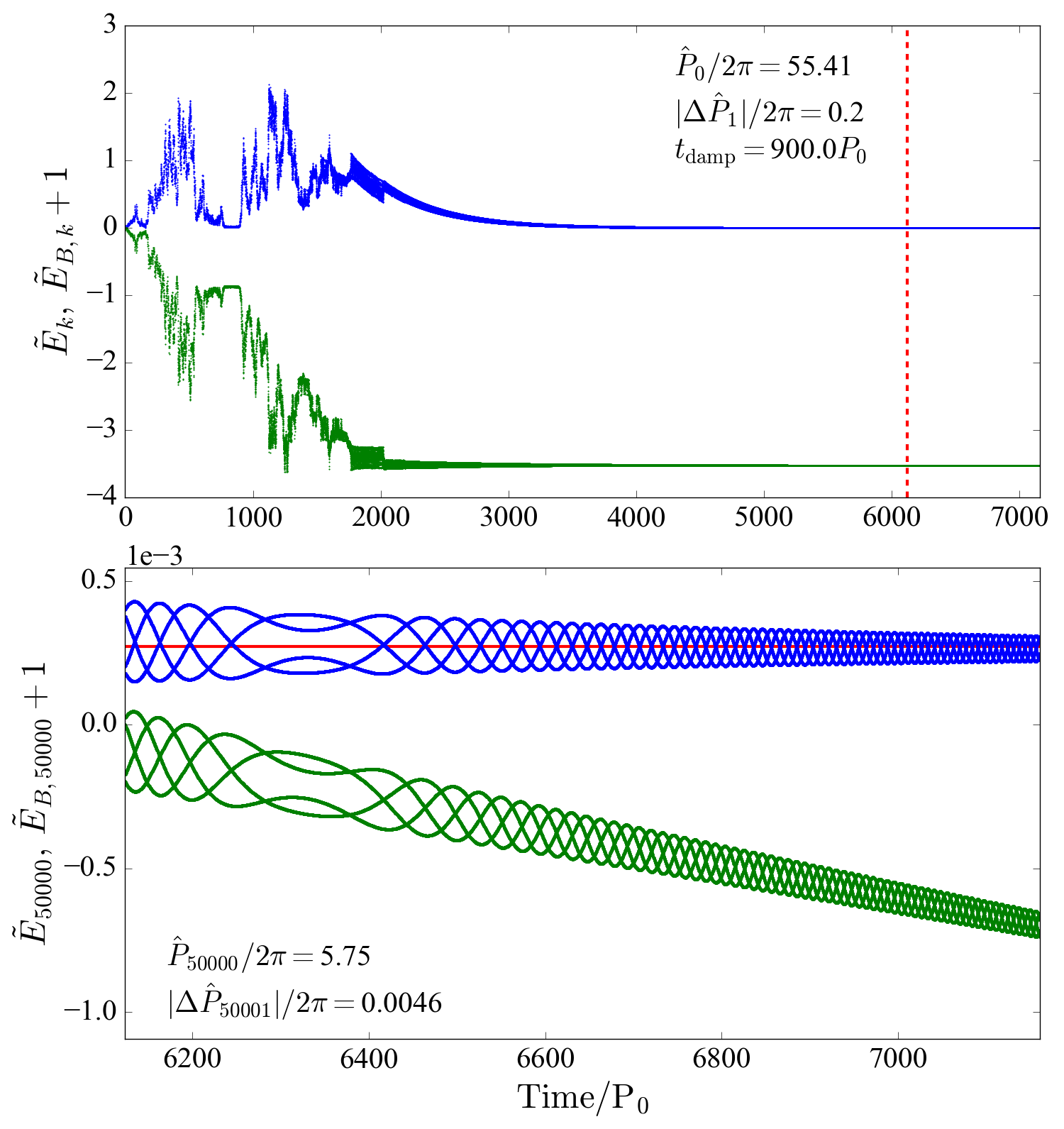
Figure 8: The mode energy (in blue) and the binary orbital energy (in green) over many pericentre passages. In the upper panel, the energy is normalized to the initial orbital energy of the binary. The mode energy undergoes chaotic evolution, and damps to a quasi-steady sate after a few $t_{\text{damp}}$. The lower panel shows the later phase of the evolution (to the right of the dashed red line in the upper panel), with the energy re-normalized to the energy of the binary after 50,000 orbits. The predicted quasi-steady state mode energy is shown as a solid red line. The values of ${\hat{P}}$ and $|\Delta{\hat{P}}|$ at 50,000 orbits are indicated. Note that because of the significant orbital decay during chaotic evolution, we use time (in units of $P_{0}$) rather than the number of orbits for the $x$-axis.

5 Systems with Multiple Modes

Our analysis can be easily generalized to systems with multiple modes (labelled by the index $\alpha$). The total energy in modes just before the $(k+1)$-th passage is ${\tilde{E}}_{k}=\sum_{\alpha}|a_{\alpha,k}|^{2}$. During a pericentre passage, the amplitude of each mode changes by $\Delta a_{\alpha}$. The total energy transferred to stellar modes in the $k$-th passage is

$$\Delta{\tilde{E}}_{k}=\sum_{\alpha}\left[|a_{\alpha,k-1}+\Delta a_{\alpha}|^{2}-|a_{\alpha,k-1}|^{2}\right].$$ (34)

As before, the orbital energy after the $k$-th passage is given by ${\tilde{E}}_{B,k}={\tilde{E}}_{B,0}-\sum_{j=1}^{k}\Delta{\tilde{E}}_{j}$. The relationship between the orbital energy and the period is given by equation (4). The mode amplitude of each mode just before the $(k+1)$-th passage is

$$a_{\alpha,k}=[a_{\alpha,k-1}+\Delta a_{\alpha}]\,\text{e}^{-(\text{i}+{\hat{\gamma}}_{\alpha}){\hat{P}}_{\alpha,k}}$$ (35)

where ${\hat{P}}_{\alpha,k}\equiv\omega_{\alpha}P_{k}$. Similarly, we define $|\Delta{\hat{P}}_{\alpha,1}|\equiv\omega_{\alpha}|\Delta P_{1}|$. The evolution of the system is completely determined by ${\hat{P}}_{\alpha,0}$, $|\Delta{\hat{P}}_{\alpha,1}|$ and ${\hat{\gamma}}_{\alpha}=\gamma_{\alpha}/\omega_{\alpha}$.

In general, systems with multiple modes exhibit the same types of behaviours seen in the single-mode system. Systems with small $|\Delta{\hat{P}}_{\alpha,1}|$ pass through multiple resonances over many orbits. For systems with many modes, resonances play a significant role in the orbital evolution, as shown in Fig. 9. Multi-mode systems also exhibit chaotic growth that damps into a quasi-steady state (see Fig. 10).

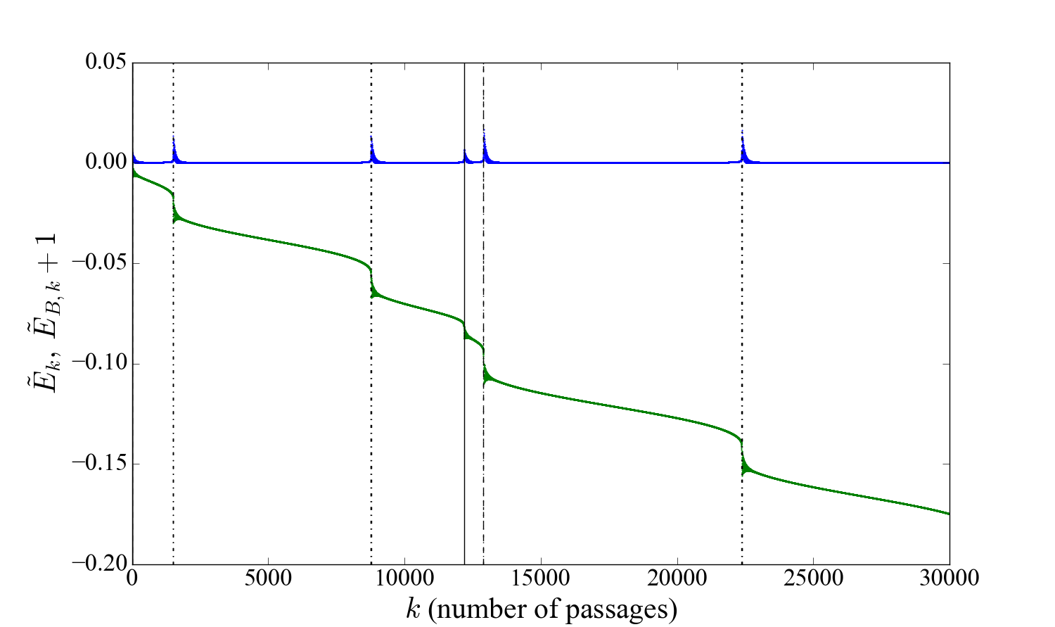
Figure 9: The total mode energy and orbital energy of a system with three modes that evolves through multiple resonances. The properties of the modes are discussed in detail in Appendix C. For this system, the parameters are ${\hat{P}}_{\alpha,0}/2\pi=123,56.6,50.4$ and $|\Delta{\hat{P}}_{\alpha,1}|/2\pi=0.1,0.05,0.04$. The mode damping times are all of order $t_{\rm{damp}}\sim 100P_{0}$. Resonances for different modes are shown with vertical solid, dashed, and dot-dashed lines.

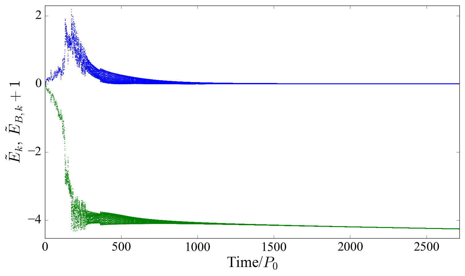
Figure 10: The total mode energy and orbital energy of a system with three modes that undergoes initial chaotic growth and eventually damps to a quasi-steady state. The properties of the modes are discussed in detail in Appendix C. For this system, the parameters are ${\hat{P}}_{\alpha,0}/2\pi=123,137,113$ and $|\Delta{\hat{P}}_{\alpha,1}|/2\pi=2.3,2.5,2.1$. The mode damping times are all of order $t_{\rm{damp}}\sim 100P_{0}$.

Figure 11 shows two examples similar to Fig. 1 that explore the parameter space of systems with three modes — one with a dominant mode, and another with $(\Delta a_{\alpha})$ roughly equal for all modes. For application to stellar binaries, the example with a dominant mode is characteristic of a binary with $M\sim(\text{a few})M_{\odot}$ and a small pericentre separation $(\eta\sim 3)$. For systems with larger $\eta$’s, the tidal potential tends to excite higher-order modes to similar amplitudes. Appendix C provides more detail on the choice of mode properties, which are determined using MESA stellar models and the non-adiabatic GYRE pulsation code (Paxton et al., 2011; Townsend & Teitler, 2013). In general, including multiple modes does not alter the classes of behaviours that the system exhibits. However, the multiple-mode model is more prone to chaotic evolution. Additionally, all modes, even those with relatively small $\Delta a_{\alpha}$ can guide the evolution of the system near resonance.

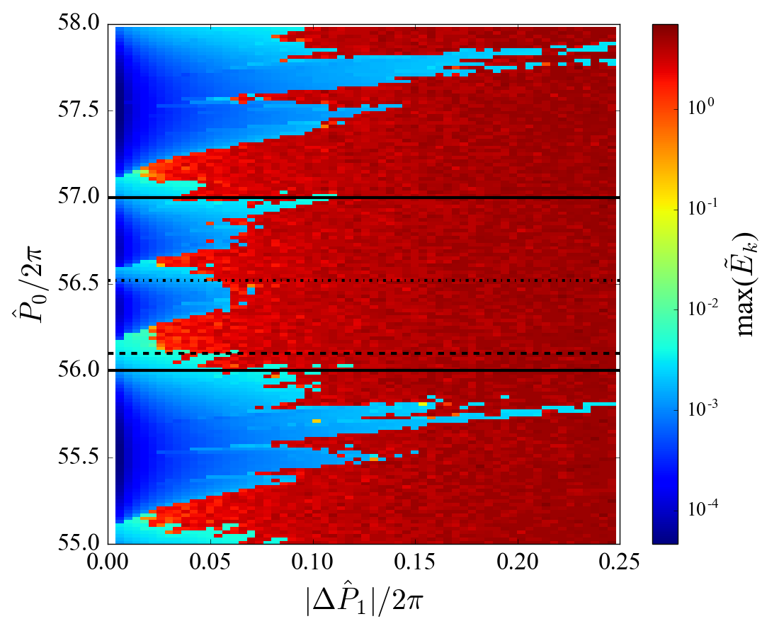
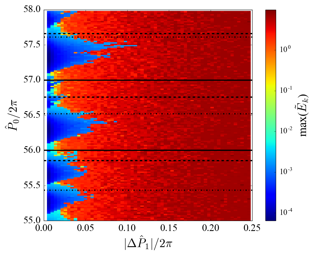
Figure 11: The maximum mode energy (summed over all modes) reached in 10,000 orbits as a function of $\omega_{1}|\Delta P_{1}|/2\pi$ and $\omega_{1}P_{0}/2\pi$. In the dark blue regions, the modes exhibit low-energy oscillations, while in the dark red regions the modes grow chaotically to large amplitudes. The left panel shows a system with one dominant mode. The frequency ratios are $\omega_{2}/\omega_{1}=0.41$ and $\omega_{3}/\omega_{1}=0.46$. The energy ratios are $\Delta{\tilde{E}}_{2,1}/\Delta{\tilde{E}}_{1,1}=0.04$ and $\Delta{\tilde{E}}_{3,1}/\Delta{\tilde{E}}_{1,1}=0.03.$ The dashed line corresponds to $\omega_{2}{\hat{P}}_{0}/2\pi=23$, the dot-dashed line to $\omega_{3}{\hat{P}}_{0}/2\pi=26$, and the solid lines to resonances for $\omega_{1}$. The right panel shows a system where all three modes are excited to similar energies. The frequency ratios are $\omega_{2}/\omega_{1}=1.11$ and $\omega_{3}/\omega_{1}=0.92$. The energy ratios are $\Delta{\tilde{E}}_{2,1}/\Delta{\tilde{E}}_{1,1}=0.94$ and $\Delta{\tilde{E}}_{3,1}/\Delta{\tilde{E}}_{1,1}=0.58$. The dashed lines corresponds to $\omega_{2}{\hat{P}}_{0}/2\pi=62,63,64$, the dot-dashed lines to $\omega_{3}{\hat{P}}_{0}/2\pi=51,52,53$, and the solid lines to resonances for $\omega_{1}$.

6 Summary and Discussion

We have developed a mathematically simple model that accurately captures the evolution of eccentric binary systems driven by dynamical tides. This model is exact for linear tidal oscillations in highly eccentric systems (see the last paragraph of Section 2 for the regime of validity of the model). The evolution of the “eccentric orbit + oscillation mode” system can be described by an iterative map, and depends on three parameters (for a single mode system): ${\hat{P}}_{0}$, $|\Delta{\hat{P}}_{1}|$ and ${\hat{\gamma}}$ [see equations (7)-(9)], corresponding to the initial orbital period, the change in orbital period during the first pericentre passage, and the damping rate of an oscillation mode. Multiple modes can be easily incorporated.

The iterative map reveals the following key findings:

• For non-dissipative systems, the mode evolution exhibits three types of behaviours, depending on the values of $|\Delta{\hat{P}}_{1}|$ and ${\hat{P}}_{0}$ (see Figs. 1 and 3):

  1. For small $|\Delta{\hat{P}}_{1}|$ and an orbital frequency far from resonance with the mode frequency (i.e. ${\hat{P}}_{0}/2\pi$ not close to an integer), the mode experiences low-amplitude oscillations with a maximum mode energy given by equation (17).
     

  2. For small $|\Delta{\hat{P}}_{1}|$ and near resonance (${\hat{P}}_{0}/2\pi$ close to an integer), the mode exhibits larger-amplitude oscillations with a maximum energy given by equation (20).
     

  3. For $|\Delta{\hat{P}}_{1}|\gtrsim 1$, the mode energy can grow chaotically (see Fig. 4), reaching a maximum of order the orbital binding energy [see equation (26)]. The chaotic mode growth can be approximately described by a diffusion model [equation (24)], although such a model would not contain the energy maximum.

• When mode dissipation is added, all systems, even those evolving chaotically, decay to a quasi-steady state (see Figs. 6-8), with the mode energy and orbital decay rate given by equations (30) and (31), respectively. Continued orbital decay is punctuated by resonances (see Section 4.2).

These results are applicable to a variety of astrophysical systems mentioned in the introduction. In particular, a tidally captured star around a compact object in dense clusters (Mardling & Aarseth, 2001) or a massive black hole, (e.g. Li & Loeb, 2013) at the centre of galaxies may experience chaotic growth of mode amplitude during multiple pericentre passages, accompanied by significant orbital decay and tidal heating. A similar evolution may occur when a giant planet (“cold Jupiter”) is excited into a high-eccentricity orbit by an external companion (a distant star or a nearby planet) via the Lidov-Kozai mechanism (Wu & Murray, 2003; Fabrycky & Tremaine, 2007; Nagasawa et al., 2008; Petrovich, 2015; Anderson et al., 2016; Muñoz et al., 2016). We have found that a $m_{p}\sim 1~{}M_{J}$ planet pushed into an orbit with pericentre distance $\lesssim 0.015$ AU and $e\gtrsim 0.95$ will enter the chaotic regime for the growth of f-modes. The planet can spend an appreciable time in the high-$e$ phase of the Lidov-Kozai cycle, allowing the mode energy to climb to a large value at which the mode becomes non-linear and suffers rapid decay. The consequence is that the planet’s orbit quickly shrinks (by a factor of a few), similar to the behaviour depicted in Fig. 8, and the system eventually enters a quasi-steady state with slow orbital decay. We suggest that this is a promising mechanism for forming eccentric warm Jupiters, whose origin remains poorly understood (Petrovich & Tremaine, 2016; Antonini et al., 2016; Huang et al., 2016; Anderson & Lai, 2017). This mechanism also speeds up the formation of hot Jupiters through high-eccentricity migration channels.

Our study has revealed a rich variety of dynamical behaviours for highly eccentric binaries undergoing tidal interactions. Nevertheless, our model is still idealized. One effect we did not include is stellar (or planetary) rotation. The qualitative behaviours of systems that undergo low-amplitude oscillations or chaotic evolution are unlikely to change with the inclusion of rotation. However, tidal spin-up of the star (and tidal heating) can directly affect the mode frequencies, giving rise to the possibility of resonance locking under some conditions, which may extend the time frame over which the orbital energy rapidly decreases (Witte & Savonije, 1999; Fuller & Lai, 2012; Burkart et al., 2012; Fuller, 2017). In addition, as noted above, our assumption of linear damping may fail in the chaotic regime; non-linear damping could lead to even more rapid orbital evolution and significant structural changes in the excited star or planet. All of these issues deserve further study.

As this paper was under review, an independent work on dynamical tides in eccentric giant planets was submitted by Wu (2017). She considers the effect of chaotic f-mode evolution (approximately diffusive evolution) on the orbits of gas giants undergoing high-eccentricity migration, assuming that the f-mode damps non-linearly when its amplitude becomes too large. Her conclusion that dynamical tides rapidly shrink the orbit, overtaking secular migration, agrees with our results and the discussion above.

Appendix A Physical Justification for the Iterative Map

We present a brief derivation of the iterative map based on the hydrodynamics of forced stellar oscillations in binaries. We consider the tidally-excited oscillations of the primary body (mass $M$ and radius $R$) by the companion of mass $M^{\prime}$. The gravitational potential produced by $M^{\prime}$ reads

$$U({\bf r},t)=-GM^{\prime}\sum_{lm}{W_{lm}r^{l}\over D^{l+1}}\,\,e^{-im\Phi(t)}Y_{lm}(\theta,\phi),$$ (36)

where ${\bf r}=(r,\theta,\phi)$ is the position vector (in spherical coordinates) relative to the centre of mass of $M$, $D(t)$ is the binary separation and $\Phi$ is the orbital true anomaly. The dominant quadrupole terms have $l=|m|=2$ and $m=0$, for which $W_{2\pm 2}=(3\pi/10)^{1/2}$ and $W_{20}=(\pi/5)^{1/2}$. For simplicity, we neglect stellar rotation [see Schenk et al. (2002); Lai & Wu (2006)]. To linear order, the response of star $M$ to the tidal forcing frequency is specified by the Lagrangian displacement ${\mbox{\boldmath$\xi$}}({\bf r},t)$. A free oscillation mode of frequency $\omega_{\alpha}$ has the form ${\mbox{\boldmath$\xi$}}_{\alpha}({\bf r},t)={\mbox{\boldmath$\xi$}}_{\alpha}({\bf r})\,e^{-i\omega_{\alpha}t}\propto e^{im\phi-i\omega_{\alpha}t}$. We carry out phase-space expansion of ${\mbox{\boldmath$\xi$}}({\bf r},t)$ in terms of the eigenmodes Schenk et al. (2002):

$$\left[\begin{array}[]{c}{\mbox{\boldmath$\xi$}}\\ {\partial{\mbox{\boldmath$\xi$}}/\partial t}\end{array}\right]=\sum_{\alpha}c_{\alpha}(t)\left[\begin{array}[]{c}{\mbox{\boldmath$\xi$}}_{\alpha}({\bf r})\\ -i\omega_{\alpha}{\mbox{\boldmath$\xi$}}_{\alpha}({\bf r})\end{array}\right].$$ (37)

The linear fluid dynamics equations for the forced stellar oscillations then reduce to the evolution equation for the mode amplitude $c_{\alpha}(t)$ (Lai & Wu, 2006):

$$\dot{c}_{\alpha}+(i\omega_{\alpha}+\gamma_{\alpha})c_{\alpha}=\frac{iGM^{\prime}W_{lm}Q_{\alpha}}{2\omega_{\alpha}D^{l+1}}\,\text{e}^{-im\Phi(t)},$$ (38)

where $\gamma_{\alpha}$ is the mode (amplitude) damping rate, and

$$Q_{\alpha}=\frac{1}{M^{1/2}R^{(l-1)}}\int d^{3}x\,\rho{\mbox{\boldmath$\xi$}}_{\alpha}^{\star}\cdot\nabla(r^{l}Y_{lm})$$ (39)

is the dimensionless tidal overlap integral. The eigenmode is normalized according to $\int d^{3}x\rho({\bf r})|{\mbox{\boldmath$\xi$}}_{\alpha}({\bf r})|^{2}=1$, which implies that $\xi$ has units of $M^{-1/2}$.

The general solution to equation (38) is

$$c_{\alpha}=\text{e}^{-(i\omega_{\alpha}+\gamma_{\alpha})t}\int_{t_{0}}^{t}\frac{iGM^{\prime}W_{lm}Q_{\alpha}}{2\omega_{\alpha}D^{l+1}}\,\text{e}^{(i\omega_{\alpha}+\gamma_{\alpha})t^{\prime}-im\Phi(t^{\prime})}\,dt^{\prime}.$$ (40)

For eccentric binaries, we can write this as a sum over multiple pericentre passages. To do so, let $t_{k}$ be the time of the $k$-th apocentre passage. [Note that, for the moment, this use of $k$ differs from the meaning used in equations (1)-(5), where it is used to describe the number of pericentre passages]. We can relate $t_{k}$ to $t_{k-1}$ via

$$t_{k}=t_{k-1}+\frac{1}{2}(P_{k-1}+P_{k}).$$ (41)

Now define

$$\Delta c_{\alpha}=\int_{-P_{k-1}/2}^{P_{k}/2}\frac{iGM^{\prime}W_{lm}Q_{\alpha}}{2\omega_{\alpha}D^{l+1}}\,\text{e}^{(i\omega_{\alpha}+\gamma_{\alpha})t^{\prime}-im\Phi(t^{\prime})}\;dt^{\prime}.$$ (42)

This is the change in mode amplitude during a pericentre passage, and it is approximately constant for any $k$ provided the orbit is very eccentric and the pericentre distance $r_{\rm{peri}}$ remains constant (see the main text for discussion). We can then write $c_{\alpha}$ at time $t_{k}$ simply as

$$c_{\alpha,k}=\text{e}^{-(i\omega_{\alpha}+\gamma_{\alpha})t_{k}}\Delta c_{\alpha}\sum_{j=1}^{k}\,e^{(i\omega_{\alpha}+\gamma_{\alpha})(t_{j-1}+P_{j-1}/2)}.$$ (43)

We can reorganize equation (43) into an iterative form

$$c_{\alpha,k}=c_{\alpha,k-1}\,e^{-(i\omega_{\alpha}+\gamma_{\alpha})(P_{k-1}+P_{k})/2}+e^{-(i\omega_{\alpha}+\gamma_{\alpha})P_{k}/2}\Delta c_{\alpha}.$$ (44)

We now shift the index $k$ to count pericentre passages rather than apocentre passages by defining

$$a_{\alpha,k}=\sqrt{2}\omega_{\alpha}c_{\alpha,k}\,\text{e}^{-i\omega P_{k}/2}/|E_{B,0}|,$$ (45)

where we have also re-normalized the mode amplitude so that the scaled mode energy (in units of $|E_{B,0}|$) is ${\tilde{E}}_{\alpha,k}=|a_{\alpha,k}|^{2}.$ (Note the mode energy is given by $E_{\alpha,k}=2\omega_{\alpha}^{2}|c_{\alpha,k}|^{2}$.) Equation (44) then reduces to

$$a_{\alpha,k}=(a_{\alpha,k-1}+\Delta a_{\alpha})\,e^{-(i\omega_{\alpha}+\gamma_{\alpha})P_{k}},$$ (46)

where $\Delta a_{\alpha}=\sqrt{2}\omega_{\alpha}\Delta c_{\alpha}/|E_{B,0}|$.

Using equation (42), we can write $\Delta E_{\alpha,1}$ explicitly in terms of orbital parameters and mode properties:

$$\Delta E_{\alpha,1}=|E_{B,0}|(\Delta a_{\alpha})^{2}=\frac{GM^{\prime 2}}{R}\left(\frac{R}{r_{\rm peri}}\right)^{2(l+1)}T(\eta,\omega_{\alpha}/\Omega_{\rm peri},e),$$ (47)

where the dimensionless function $T$ is given by

$$T=2\pi^{2}Q_{\alpha}^{2}K_{lm}^{2}.$$ (48)

Ignoring the negligible effect of mode damping at pericentre, we have

$$K_{lm}=\frac{W_{lm}}{2\pi}\left(\frac{GM}{R^{3}}\right)^{1/2}\int_{-P/2}^{P/2}dt^{\prime}\left(\frac{r_{\rm peri}}{D}\right)^{l+1}\text{e}^{\text{i}\omega_{\alpha}t^{\prime}-im\Phi(t^{\prime})}.$$ (49)

The energy transfer for a parabolic passage $(e\to 1)$ was first derived in Press & Teukolsky (1977). Equations (47)-(49), which apply to eccentric orbits as well, were presented in Lai (1997) [see equations (22)-(23)] and in Fuller & Lai (2012) [see equation (14)-(15); note that in equation (15), $R$ should be replaced by $D_{p}$.]

Note that the integral in equation (49) is difficult to calculate accurately and efficiently because the mode frequency is typically orders of magnitude larger than the orbital frequency. However, for parabolic orbits, $K_{lm}$ can be evaluated in the limit $\omega_{\alpha}/\Omega_{\rm peri}\gg 1$ (Lai, 1997). For example, for $l=2$, $m=2$,

$$K_{22}=\frac{2z^{3/2}\eta^{3/2}\text{e}^{-2z/3}}{\sqrt{15}}\left(1-\frac{\sqrt{\pi}}{4\sqrt{z}}+\cdots\right),$$ (50)

where

$$z\equiv\sqrt{2}\omega_{\alpha}/\Omega_{\rm peri}.$$ (51)

This expansion approximates $K_{lm}$ to within a few percent for $(1-e)<<1$ and $z\gtrsim 3$. For typical f-mode frequencies, the latter condition is satisfied for $\eta\gtrsim$ a few.

Appendix B Non-dissipative Systems

B.1 Maximum Mode Energy for Non-Chaotic Systems

In the oscillatory and resonant regimes, the mode energy $\tilde{E}_{k}\ll 1$, and the iterative map given by equation (19) can be rewritten:

$$z_{k+1}\simeq 1+z_{k}\,e^{-i{\hat{P}}_{0}+i|\Delta{\hat{P}}_{1}||z_{k}|^{2}},$$ (52)

where $z_{k}\equiv a_{k-}/\Delta a=a_{k-1}/\Delta a+1$.

Oscillatory Regime: When $|\delta{\hat{P}}_{0}|=|{\hat{P}}_{0}-2\pi N|\gg|\Delta{\hat{P}}_{1}||z_{k}|^{2}$, the map simplifies to

$$z_{k+1}\simeq 1+z_{k}\,e^{-i{\hat{P}}_{0}}.$$ (53)

This yields the solution (for $z_{1}=1$)

$$z_{k}\simeq{1-e^{-ik{\hat{P}}_{0}}\over 1-e^{-i{\hat{P}}_{0}}},$$ (54)

which is equivalent to equation (16). The validity of this oscillatory solution requires $|\delta{\hat{P}}_{0}|\gg|\Delta{\hat{P}}_{1}|/(1-\cos{\hat{P}}_{0})$ or $|\delta{\hat{P}}_{0}|^{3}\gg|\Delta{\hat{P}}_{1}|$.

Resonant Regime: When $|\delta{\hat{P}}_{0}|^{3}\ll|\Delta{\hat{P}}_{1}|$, the system is in the resonant regime, and the map becomes

$$z_{k+1}-z_{k}\simeq 1+i|\Delta{\hat{P}}_{1}||z_{k}|^{2}z_{k}.$$ (55)

For $k\gg 1$, we can approximate the mode amplitude as a continuous function of $k$, and the above equation reduces to

$$\frac{dz}{dk}\simeq 1+i|\Delta{\hat{P}}_{1}||z|^{2}z.$$ (56)

Now we express $z$ explicitly in terms of an amplitude $A$ and phase $\theta$:

$$z=A\,\text{e}^{\text{i}\theta}.$$ (57)

Equation (56) can be rewritten as two differential equations:

$$\frac{dA}{dk} \simeq\cos\theta,$$ (58)

$$\frac{d\theta}{dk} \simeq\frac{1}{A}\left(|\Delta{\hat{P}}_{1}|A^{3}-\sin\theta\right).$$ (59)

We combine these to examine how the amplitude varies with the phase:

$$\frac{dA}{d\theta}=\frac{A\cos\theta}{\left(|\Delta{\hat{P}}_{1}|A^{3}-\sin\theta\right)}.$$ (60)

To solve the above equation, we use the substitutions

$$u=|\Delta{\hat{P}}_{1}|A^{3},\quad v=\sin\theta.$$ (61)

Equation (60) then simplifies to

$$\frac{du}{dv}=\frac{3u}{u-v}.$$ (62)

For the initial condition $u=v=0$, which corresponds to $a_{0}=0$, the solution is simply $u=4v$, or

$$A=\left(\frac{4\sin\theta}{|\Delta{\hat{P}}_{1}|}\right)^{1/3},$$ (63)

which has the maximum value $(4/|\Delta{\hat{P}}_{1}|)^{1/3}$. The maximum mode energy for a system near resonance is therefore

$${\tilde{E}}_{\rm res}\equiv\tilde{E}_{k,\text{max}}=(\Delta a)^{2}\left(\frac{4}{|\Delta{\hat{P}}_{1}|}\right)^{2/3}\simeq\frac{2^{7/3}}{3}{|\Delta{\hat{P}}_{1}|^{1/3}\over{\hat{P}}_{0}}.$$ (64)

We can use the above result to approximate the shape that the mode amplitude traces in the complex plane over many orbits. Our numerical calculation (see Fig. 3) shows that the mode amplitude as a function of its phase can be described by

$$\left|\frac{a_{k}}{\Delta a}+0.5\right|\simeq\left(\frac{4\sin\theta}{|\Delta{\hat{P}}_{1}|}\right)^{1/3},$$ (65)

where $\theta$ is the phase of $a_{k}/\Delta a+0.5$. This is similar to equation (63) except for a shift along the real axis. For $|\Delta{\hat{P}}_{1}|\ll 1$, this approximation performs very well, as seen in Fig. 3.

B.2 Resonant Timescale

The mode of a non-dissipative system near resonance evolves periodically, repeatedly tracing out a closed shape in the complex amplitude plane. We define $t_{\text{res}}$ as the period of the resonant oscillations. To calculate this timescale, we use equations (58) and (63) to find

$$\frac{d\theta}{dk}\simeq\left(\frac{|\Delta{\hat{P}}_{1}|}{4}\right)^{\!1/3}3(\sin\theta)^{2/3}.$$ (66)

Integrating the above differential equation from $\theta=0$ to $\theta=\pi$ gives

$$t_{\text{res}}\simeq 3.85\;P|\Delta{\hat{P}}_{1}|^{-1/3},$$ (67)

where $P$ is the orbital period associated with the resonance. In order of magnitude, the number of orbits necessary to reach the maximum mode amplitude $|a_{\text{res}}|\sim|\Delta{\hat{P}}_{1}|^{-1/3}\Delta a$ is simply $|a_{\rm{res}}|/\Delta a$.

B.3 Maximum Mode Energy for Chaotic Systems

As discussed in the main text, the mode energy of a chaotic system initially grows stochastically with an expected value of $\langle{\tilde{E}}_{k}\rangle\sim\Delta{\tilde{E}}_{1}k$ [see equation (24) and Fig. 5], but cannot exceed a maximum value, ${\tilde{E}}_{\rm{max}}$. As the mode energy increases, the change in the orbital period between pericentre passages, $\Delta\hat{P}_{k}$, decreases [see equation (25)]. The maximum mode energy is approximately set by $|\Delta{\hat{P}}_{k}|\sim 1$, and is given by equation (26).

This condition is related to that found in Mardling (1995a, b), where the maximum mode energy is set by a “chaos boundary" that separates orbital parameters that produce chaotic behaviour from those that produce oscillatory behaviour. The location of the boundary depends on the current mode amplitude. The iterative map in this paper demonstrates that such boundaries are determined by the size of $|\Delta{\hat{P}}_{k}|$, which depends on $\Delta a$ and $a_{k-1}$ [see equation (25)]. Both the onset of chaotic behaviour and the maximum mode energy are set by conditions on $|\Delta{\hat{P}}_{k}|$ (where $k=1$ when considering the onset). It follows that both conditions are related to “chaos boundaries", as observed by Mardling (1995a, b).

In reality, the dependence of ${\tilde{E}}_{\rm{max}}$ on ${\hat{P}}_{0}$ and $|\Delta{\hat{P}}_{1}|$ is more complicated than the power law trend from equation (26). Figures 12 and 13 show “jumps" and “drops" in ${\tilde{E}}_{\rm{max}}$ at some values of ${\hat{P}}_{0}$ and $|\Delta{\hat{P}}_{1}|$. To understand this step-like behaviour, we note that the maximum mode energy for a non-dissipative system is associated with the minimum (dimensionless) orbital period by

$${\hat{P}}_{\rm{min}}={\hat{P}}_{0}\left(\frac{1}{1+{\tilde{E}}_{\rm{max}}}\right)^{3/2}.$$ (68)

We have found that for a chaotic system, as $|\Delta{\hat{P}}_{k}|$ decreases toward unity, the orbital period tends to evolve away from resonances with the stellar mode and to linger directly between them. This behaviour can be understood from the fact that, for a system near resonance, the shifts in mode amplitude during pericentre tend to add over successive passages, pushing the system away from the resonance. Imposing ${\hat{P}}_{\rm{min}}\simeq 2\pi(N+1/2)$ yields

$${\tilde{E}}_{\rm{max}}\simeq\left[\frac{{\hat{P}}_{0}}{2\pi(N+1/2)}\right]^{2/3}-1.$$ (69)

Equation (69) is in good agreement with results shown in Figs. 12 and 13. We see that the jumps in ${\tilde{E}}_{\rm{max}}$ correspond to changes in $N$. Combining equation (69) with the broader trend of equation (26) captures the main features of how ${\tilde{E}}_{\rm{max}}$ depends on ${\hat{P}}_{0}$ and $|\Delta{\hat{P}}_{1}|$ for chaotic systems.

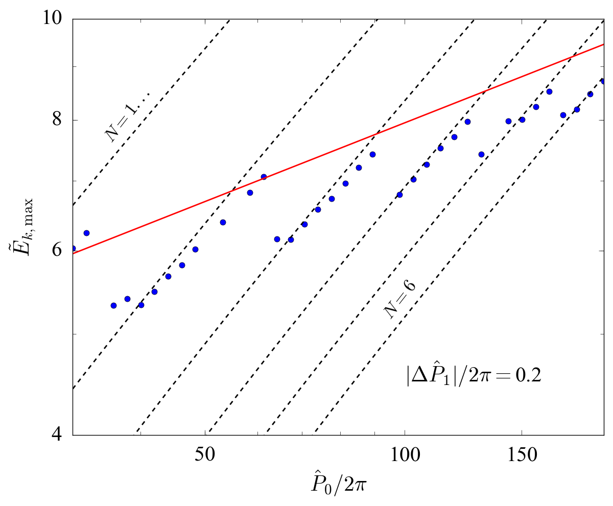
Figure 12: Numerical results for $\tilde{E}_{\rm{max}}$ (blue dots) after $3\times 10^{6}$ orbits for chaotic systems with $|\Delta\tilde{P}_{1}|/2\pi=0.2$. The red line is $1.5({\hat{P}}_{0}|\Delta{\hat{P}}_{1}|)^{1/4}$ [see equation (26)]. The dotted lines are from equation (69) with different values of $N$.

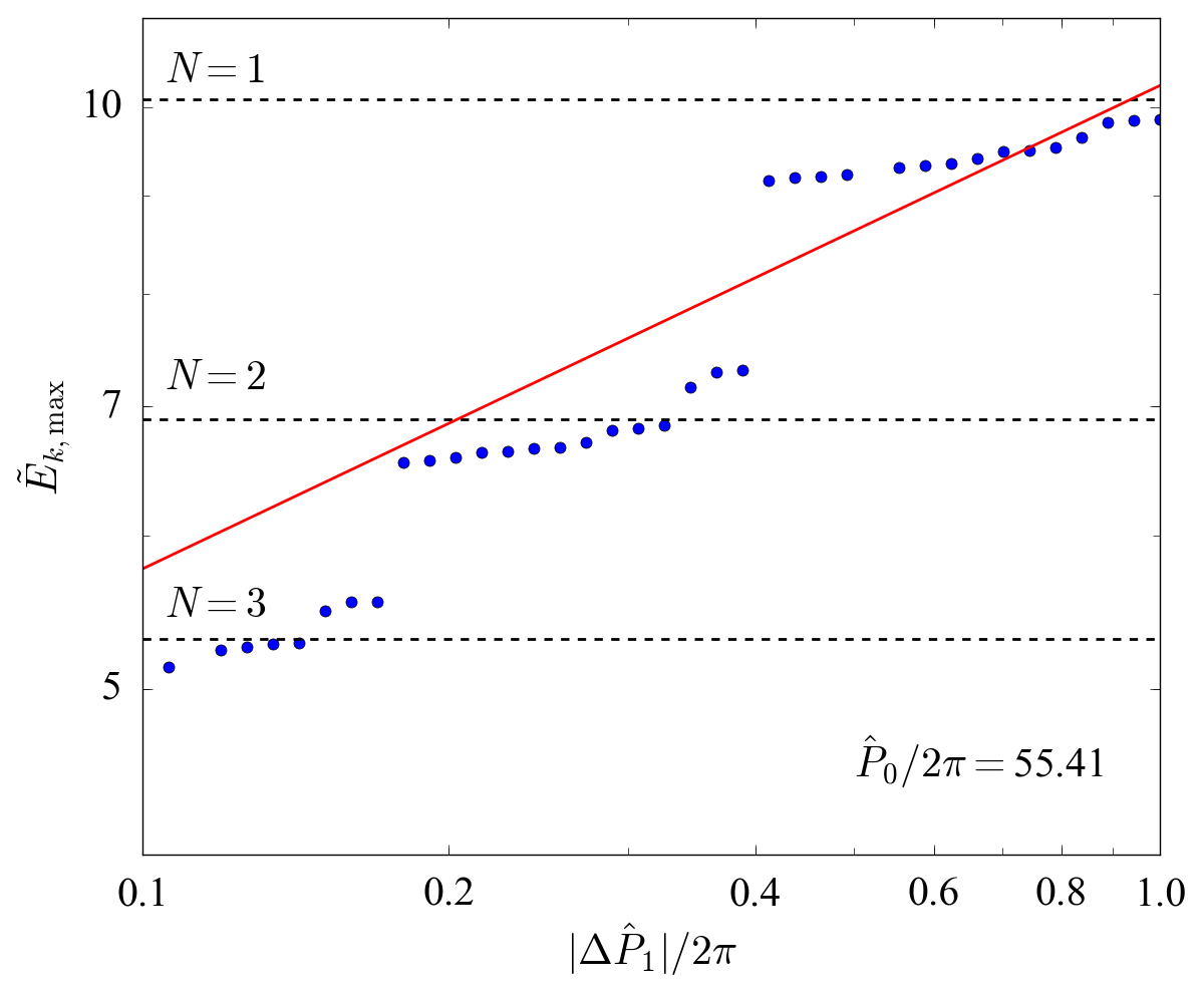
Figure 13: Numerical results for $\tilde{E}_{\rm{max}}$ (blue dots) after $3\times 10^{6}$ orbits for chaotic systems with ${\hat{P}}_{0}/2\pi=55.41$. The red line is $1.5({\hat{P}}_{0}|\Delta{\hat{P}}_{1}|)^{1/4}$ [see equation (26)]. The dotted lines are from equation (69 with different values of $N$).

Appendix C G-mode Properties of Stellar Models

One application of our model is the tidal capture of main-sequence stars by compact objects, including massive black holes. We use the stellar evolution code, MESA (Paxton et al., 2011), and the non-adiabatic pulsation code, GYRE (Townsend & Teitler, 2013), to determine the properties of g-modes in the radiative envelope of stars between $2$ and $10M_{\odot}$. The characteristic damping times of modes are found using the imaginative part of the mode frequency. These values are generally in good agreement with a quasi-adiabatic approximation that assumes radiative damping. Figure 14 shows the computed damping rates for three stellar models. For the $2M_{\odot}$ model, the damping rate only varies by a factor of a few for the relevant g-modes. For the $10M_{\odot}$ model (and other models with $10M_{\odot}\leq M\leq 20M_{\odot}$), the damping rates are much smaller for higher frequency modes.

The amount of energy transferred to a mode (labelled $\alpha$) in the “first” pericentre passage $\Delta E_{\alpha,1}$ (i.e., when the oscillation amplitude is zero before the passage) depends on the stellar structure and mode properties. We use the method of Press & Teukolsky (1977) to calculate $\Delta E_{\alpha,1}$. The quasi-steady-state mode dissipation rate from equation (30) is of order $\gamma_{\alpha}\Delta E_{\alpha,1}$. Figure 15 shows an example of the calculated $\Delta E_{\alpha,1}$ and the energy dissipation rates for systems with different stellar properties and $\eta=3$. We find that stars with $M\lesssim 5M_{\odot}$ tend to have a single low-order g-mode with large $\Delta{\tilde{E}}_{\alpha,1}$ that dominates the energy transfer rate. To represent a system with a dominant mode, we choose the $\omega$ and $\gamma$ ratios between modes from the $2M_{\odot}$ model and the ${\tilde{E}}_{\alpha,1}$ ratio for $\eta=3$. More massive stars ($M\gtrsim M_{\odot}$) have a number of g-modes that contribute roughly equally to the energy transfer rate. To represent a system where multiple modes are important for energy transfer, we choose the $\omega$ and $\gamma$ ratios between modes from the $10M_{\odot}$ model and the ${\tilde{E}}_{\alpha,1}$ ratio for $\eta=3$.

The orbital parameter $\eta=(r_{\rm{peri}}/R)(M/M_{t})^{1/3}$ (where $r_{\rm{peri}}$ is the pericentre distance) also strongly affects $\Delta E_{\alpha,1}$, though the dependence on $e$ is negligible for highly eccentric orbits. For larger $\eta$, the orbital frequency at pericentre is smaller, and higher-order g-modes contribute more to tidal energy transfer, as illustrated in Fig. 16.

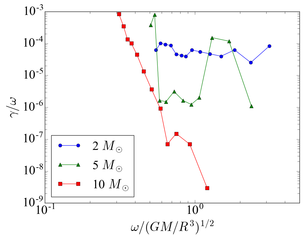
Figure 14: Numerical results for the g-mode frequencies ($\omega$) and damping rates ($\gamma$) of three MESA stellar models analysed with the non-adiabatic stellar pulsation code, GYRE. The dip in $\gamma/\omega$ for the $5M_{\odot}$ model is typical for models in the mass range $4-8M_{\odot}$.

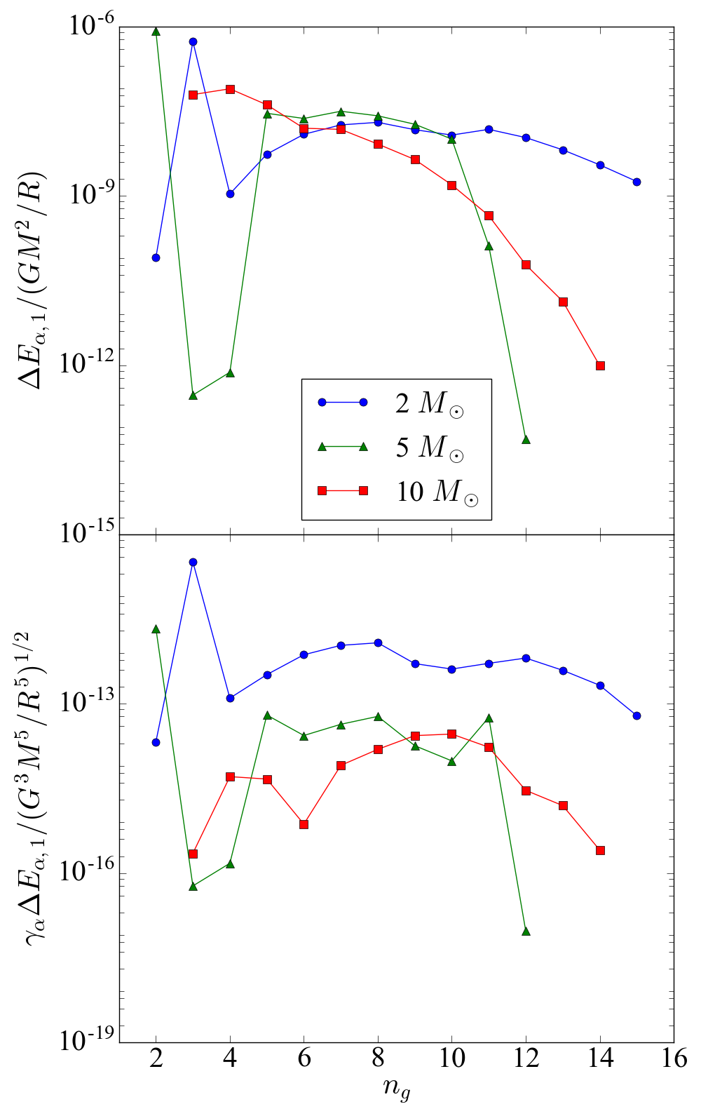
Figure 15: Numerical results for $\Delta E_{\alpha,1}$ and $\gamma_{\alpha}\Delta E_{\alpha,1}$ vs. $n_{g}$ (the radial mode number) for three MESA stellar models analysed with the non-adiabatic stellar pulsation code, GYRE. The energy transfer $\Delta E_{\alpha,1}$ is calculated assuming $\eta=3$ and $e=0.95$.

Figure 16: Numerical results for $\Delta E_{\alpha,1}$ for four g-modes of the $10M_{\odot}$ stellar model as a function of $\eta$. For larger $\eta$, higher order g-modes receive more energy at pericentre than lower-order g-modes.

References

- Anderson & Lai (2017) Anderson K. R., Lai D., 2017, preprint, (arXiv:1706.00084)
- Anderson et al. (2016) Anderson K. R., Storch N. I., Lai D., 2016, MNRAS, 456, 3671
- Antonini et al. (2016) Antonini F., Hamers A. S., Lithwick Y., 2016, AJ, 152, 174
- Beck et al. (2014) Beck P. G., et al., 2014, A&A, 564, A36
- Burkart et al. (2012) Burkart J., Quataert E., Arras P., Weinberg N. N., 2012, MNRAS, 421, 983
- Fabian et al. (1975) Fabian A. C., Pringle J. E., Rees M. J., 1975, MNRAS, 172, 15p
- Fabrycky & Tremaine (2007) Fabrycky D., Tremaine S., 2007, ApJ, 669, 1298
- Fuller (2017) Fuller J., 2017, MNRAS, 470, 1642
- Fuller & Lai (2012) Fuller J., Lai D., 2012, MNRAS, 420, 3126
- Guillochon (2016) Guillochon J., 2016, Catalog of Possible Tidal Disruption Events, https://astrocrash.net/resources/tde-catalogue/
- Huang et al. (2016) Huang C., Wu Y., Triaud A. H. M. J., 2016, ApJ, 825, 98
- Ivanov & Papaloizou (2004) Ivanov P. B., Papaloizou J. C. B., 2004, MNRAS, 347, 437
- Ivanov & Papaloizou (2007) Ivanov P. B., Papaloizou J. C. B., 2007, MNRAS, 376, 682
- Ivanov & Papaloizou (2011) Ivanov P. B., Papaloizou J. C. B., 2011, Celestial Mechanics and Dynamical Astronomy, 111, 51
- Kirk et al. (2016) Kirk B., et al., 2016, AJ, 151, 68
- Kochanek (1992) Kochanek C. S., 1992, ApJ, 385, 604
- Kumar & Goodman (1996) Kumar P., Goodman J., 1996, ApJ, 466, 946
- Lai (1996) Lai D., 1996, ApJ, 466, L35
- Lai (1997) Lai D., 1997, ApJ, 490, 847
- Lai & Wu (2006) Lai D., Wu Y., 2006, Phys. Rev. D, 74, 024007
- Lee & Ostriker (1986) Lee H. M., Ostriker J. P., 1986, ApJ, 310, 176
- Li & Loeb (2013) Li G., Loeb A., 2013, MNRAS, 429, 3040
- MacLeod et al. (2014) MacLeod M., Goldstein J., Ramirez-Ruiz E., Guillochon J., Samsing J., 2014, ApJ, 794, 9
- Mardling (1995a) Mardling R. A., 1995a, ApJ, 450, 722
- Mardling (1995b) Mardling R. A., 1995b, ApJ, 450, 732
- Mardling & Aarseth (2001) Mardling R. A., Aarseth S. J., 2001, MNRAS, 321, 398
- Muñoz et al. (2016) Muñoz D. J., Lai D., Liu B., 2016, MNRAS, 460, 1086
- Nagasawa et al. (2008) Nagasawa M., Ida S., Bessho T., 2008, ApJ, 678, 498
- Paxton et al. (2011) Paxton B., Bildsten L., Dotter A., Herwig F., Lesaffre P., Timmes F., 2011, ApJS, 192, 3
- Petrovich (2015) Petrovich C., 2015, ApJ, 799, 27
- Petrovich & Tremaine (2016) Petrovich C., Tremaine S., 2016, ApJ, 829, 132
- Press & Teukolsky (1977) Press W. H., Teukolsky S. A., 1977, ApJ, 213, 183
- Rees (1988) Rees M. J., 1988, Nature, 333, 523
- Schenk et al. (2002) Schenk A. K., Arras P., Flanagan É. É., Teukolsky S. A., Wasserman I., 2002, Phys. Rev. D, 65, 024001
- Stone & Metzger (2016) Stone N. C., Metzger B. D., 2016, MNRAS, 455, 859
- Stone et al. (2017) Stone N. C., Küpper A. H. W., Ostriker J. P., 2017, MNRAS, 467, 4180
- Thompson et al. (2012) Thompson S. E., et al., 2012, ApJ, 753, 86
- Townsend & Teitler (2013) Townsend R. H. D., Teitler S. A., 2013, MNRAS, 435, 3406
- Vick et al. (2017) Vick M., Lai D., Fuller J., 2017, MNRAS, 468, 2296
- Welsh et al. (2011) Welsh W. F., et al., 2011, ApJS, 197, 4
- Witte & Savonije (1999) Witte M. G., Savonije G. J., 1999, A&A, 350, 129
- Wu (2017) Wu Y., 2017, preprint, (arXiv:1710.02542)
- Wu & Murray (2003) Wu Y., Murray N., 2003, ApJ, 589, 605