Spontaneous symmetry breaking of fundamental states, vortices, and dipoles in two- and one-dimensional linearly coupled traps with cubic self-attraction

Abstract

We introduce two- and one-dimensional (2D and 1D) systems of two linearly-coupled Gross-Pitaevskii equations (GPEs) with the cubic self-attraction and harmonic-oscillator (HO) trapping potential in each GPE. The system models a Bose-Einstein condensate with a negative scattering length, loaded in a double-pancake trap, combined with the in-plane HO potential. In addition to that, the 1D version applies to the light transmission in a dual-core waveguide with the Kerr nonlinearity and in-core confinement represented by the HO potential. The subject of the analysis is spontaneous symmetry breaking in 2D and 1D ground-state (GS, alias fundamental) modes, as well as in 2D vortices and 1D dipole modes (the latter ones do not exist without the HO potential). By means of the variational approximation and numerical analysis, it is found that both the 2D and 1D systems give rise to a symmetry-breaking bifurcation (SBB) of the supercrtical type. Stability of symmetric states and asymmetric ones, produced by the SBB, is analyzed through the computation of eigenvalues for perturbation modes, and verified by direct simulations. The asymmetric GSs are always stable, while the stability region for vortices shrinks and eventually disappears with the increase of the linear-coupling constant, $\kappa$. The SBB in the 2D system does not occur if $\kappa$ is too large (at $\kappa>\kappa_{\max}$); in that case, the two-component system behaves, essentially, as its single-component counterpart. In the 1D system, both asymmetric and symmetric dipole modes feature an additional oscillatory instability, unrelated to the symmetry breaking. This instability occurs in several regions, which expand with the increase of $\kappa$.

I Introduction

A basic principle of the guided wave propagation in linear media is that the ground state (GS) in such systems exactly follows the symmetry of the guiding potential, while the first excited state features the opposite parity. In particular, the GS of a quantum particle trapped in a double-well potential is always symmetric, with respect to the potential structure, while the wave function of the first excited state is antisymmetric LL . Beyond the framework of the linear propagation, Bose-Einstein condensates (BECs) are modeled by the Gross-Pitaevskii equation (GPE), which contains the cubic term representing repulsive or attractive interactions between atoms BEC . Similar nonlinear Schrödinger equations (NLSEs), usually with the cubic self-focusing (Kerr) nonlinearity, are well known as models of the guided light transmission in optics NLS .

It is well known too that, if the GPE or NLSE contains a symmetric trapping potential, the GS wave function follows its symmetry only if the strength of the self-attractive nonlinearity does not exceed a certain critical level. Above it, effects of the spontaneous symmetry breaking kick in, destabilizing the symmetric state and replacing it, as the GS, by an asymmetric wave function. These effects were originally predicted in early works early , and have then drawn much attention, due to their obvious physical interest. In particular, they have been studied in detail in one-dimensional (1D) dual-core systems, which represent nonlinear twin-core optical waveguides bif1D , modeled by a pair of linearly coupled NLSEs. A similar system of 1D linearly coupled GPEs may be realized as the model of a pair of parallel cigar-shaped traps, filled by self-attractive BEC and linearly coupled by tunneling of atoms HS . The latter model is a natural extension of the single GPE with a double-well potential double-well-BEC . In these systems, a basic problem is the spontaneous symmetry breaking in two-component solitons (nonlinear confined modes), through the phase transitions of the first or second kind, alias sub- and supercritical bifurcations, respectively bif . Experimentally, spontaneous symmetry breaking has been demonstrated, in particular, in lasing realized in various nonlinear-optical settings lasers , in BEC loaded in a double-well potential trap Markus , and in optical metamaterials Kivshar .

Many theoretical and experimental results on the topic of the spontaneous symmetry breaking in various nonlinear systems, chiefly in the 1D geometry, have been collected in a recently published volume book (see also a review in Ref. review ). Fewer theoretical results have been reported about symmetry-breaking bifurcations (SBBs) in 2D systems. In the absence of trapping potentials, the SBB of 2D two-component solitons was studied in the model of the spatiotemporal light propagation in a dual-core waveguide with the intrinsic cubic-quintic nonlinearity Nir (see also Ref. Gena ), which was adopted to prevent destruction of the solitons by the collapse CQ . The analysis was performed for fundamental solitons, with zero vorticity ($S=0$), as well for the spatiotemporal vortex solitons, with $S=1$ (cf. Ref. X , as concerns the latter concept). The SBB for 2D fundamental and vortex solitons in a two-layer BEC, supported by the lattice potential acting in both layers, was studied in Ref. Arik .

In this work, we aim to propose a sufficiently fundamental setting for the study of the symmetry-breaking phenomenology in the 2D geometry: a system of two linearly-coupled GPEs with the cubic self-attraction and an isotropic harmonic-oscillator (HO) potential. It directly applies to the BEC with a negative scattering, loaded in a combination of a planar double-pancake trap and in-plane HO potential, the linear coupling being provided by tunneling of atoms between the parallel “pancakes”. We also consider a 1D version of this system, which additionally applies to the spatial-domain light propagation in dual-core planar optical waveguides. This setting was largely unexplored, except for Ref. sala-boris . However, the model considered in that work was essentially different, as it was based on 2D mean-field equations for dense condensates, which include the GPE nonlinearly coupled to an additional equation for the transverse width of the quasi-2D layer, i.e., the 2D version of the nonpolynomial Schrödinger equation (NPSE) Luca . As a result, the collapse area in the parameter space of the coupled NPSEs, found in Ref. Luca , is much larger than in the system of the coupled GPEs considered here. Another essential difference is that the instability of vortices against splitting was only mentioned, but not studied in Ref. Luca , while the present paper studies it in detail, see Fig. 13 below.

The model is introduced in Section II. It is followed by the consideration of the symmetry-breaking of 2D confined states, with $S=0$ and $S=1$, in Sections II and III, by means of the variational approximation (VA) and numerical methods, respectively. The respective SBB is identified as a supercritical one, and stability regions for symmetric and asymmetric 2D fundamental and vortex modes are found. In the 1D system, the SBB and stability are addressed for the GS solutions and dipole modes, i.e., the lowest excited states; unlike the GSs and vortices, the 1D dipoles do not exist in the absence of the HO potential. The paper is concluded by Section IV.

II The model

II.1 The two-dimensional setting

We consider the system of two linearly coupled 2D GPEs for complex wave functions $\phi\left(x,y,t\right)$ and $\psi\left(x,y,t\right)$ with the cubic self-attractive nonlinearity and HO trapping potential, written in the usual scaled form:

$$i\phi_{t} = -\frac{1}{2}\left(\phi_{xx}+\phi_{yy}\right)-|\phi|^{2}\phi+\frac{1}{2}\left(x^{2}+y^{2}\right)\phi-\kappa\psi,$$ (1)

$$i\psi_{t} = -\frac{1}{2}\left(\psi_{xx}+\psi_{yy}\right)-|\psi|^{2}\psi+\frac{1}{2}\left(x^{2}+y^{2}\right)\psi-\kappa\phi.$$ (2)

The coefficients in front of the Laplacian, cubic term, and HO potential are set equal to $1$ by means of rescaling, the single irreducible parameter being the linear-coupling coefficient, $\kappa>0$ (naturally, we assume that the scattering lengths, i.e., strengths of the nonlinear terms, are equal in both components). Equations (1) and (2) can be easily derived from the underlying 3D GPE by imposing a strong confinement along the third direction ($z$ axis), corresponding to the double-pancake configuration, and a factorized Gaussian wave function in the $z$ direction around each local maximum, with the width equal to the characteristic harmonic length sala-boris .

It is relevant to relate scaled units in which Eqs. (1) and (2) are written to their physical counterparts. Assuming the gas of ⁷Li atoms, with scattering length $\sim-0.1$ nm, which typically corresponds to the attractive interactions Hulet , the transverse confinement provided by the harmonic-oscillator potential with strength $\omega_{\perp}\sim 10$ KHz, and in-plane potential [in Eqs. (1) and (2)] with much smaller strength, $\Omega\sim 100$ Hz, the corresponding transverse and in-plane confining radii being, respectively, $r_{\perp}\sim 1$ $\mathrm{\mu}$m and $10$ $\mathrm{\mu}$m, the scaled length and time units in Eqs. (1) and (2) translate into $\sim 10$ $\mathrm{\mu}$m and $100$ ms, respectively. Thus, typical radii of the fundamental and vortex modes presented below, which are $\sim 3$ in the scaled units, correspond $\sim 30$ $\mathrm{\mu}$m in physical units. Further, the actual number of atoms in the condensate, $\mathcal{N}$, is related to the scaled norm of the wave function [see Eq. (9) below] by formula

$$\mathcal{N}\sim 10^{3}N,$$ (3)

hence the SBB, which is shown below to take place at $N\gtrsim 3$, implies that the condensate must contain, at least, $\sim 3000$ atoms. In the 1D case considered below, estimates for the physical time and length units are essentially the same, while the relation between the actual number of atoms in the quasi-1D condensate and its scaled norm is $\mathcal{N}\sim 10^{2}N$, instead of Eq. (3).

Stationary solutions to Eqs. (1) and (2) with real chemical potential $\mu$ are looked for as

$$\left\{\phi,\psi\right\}=e^{-i\mu t+iS\theta}\left\{\Phi_{S}(r),\Psi_{S}(r)\right\},$$ (4)

where $\left(r,\theta\right)$ are the polar coordinates, $S=0,1,2,...$ is the vorticity old , and real functions $\Phi_{S}$ and $\Psi_{S}$ are determined as solutions of coupled ordinary differential equations, with the prime standing for $d/dr$:

$$\mu\Phi_{S} = -\frac{1}{2}\left(\Phi_{S}^{\prime\prime}+\frac{1}{r}\Phi_{S}^{\prime}-\frac{S^{2}}{r^{2}}\Phi_{S}\right)-\Phi_{S}^{3}+\frac{1}{2}r^{2}\Phi_{S}-\kappa\Psi_{S},$$ (5)

$$\mu\Psi_{S} = -\frac{1}{2}\left(\Psi_{S}^{\prime\prime}+\frac{1}{r}\Psi_{S}^{\prime}-\frac{S^{2}}{r^{2}}\Psi_{S}\right)-\Psi_{S}^{3}+\frac{1}{2}r^{2}\Psi_{S}-\kappa\Phi_{S}.$$ (6)

Symmetric solutions, with $\phi=\psi$, are governed by the single equation,

$$i\phi_{t}=-\frac{1}{2}\left(\phi_{xx}+\phi_{yy}\right)-|\phi|^{2}\phi+\frac{1}{2}\left(x^{2}+y^{2}\right)\phi-\kappa\phi.$$ (7)

On the other hand, in the limit of $\mu\rightarrow-\infty$ the small component of an extremely asymmetric solution is given by the relation following from Eq. (6),

$$\Psi_{S}\approx-\left(\kappa/\mu\right)\Phi_{S},$$ (8)

with solution $\Phi_{S}$ given by Eq. (5) in which term $\kappa\Psi_{S}$ is omitted.

A crucially important issue is stability of solutions to Eqs. (1) and (2). In particular, antisymmetric states, with $\phi=-\psi$, are unstable, as $\kappa>0$ implies that they have a positive, rather than negative, coupling energy. Further, known facts are that all the solutions of the single equation (7) with $S=0$ are stable, and a part of vortices with $S=1$ are stable too, while all vortices with $S\geq 2$ are unstable Dum ; HSaito . Therefore, in what follows below we consider only two cases, $S=0$ (fundamental modes) and $S=1$ (unitary vortices).

The basic objective of the analysis is to find an SBB which destabilizes the symmetric states and replaces them by nontrivial stable asymmetric ones, if the total norm of the given state, $N$, exceeds a certain critical value:

$$N=N_{\phi}+N_{\psi}\equiv 2\pi\int_{0}^{\infty}\Phi_{S}^{2}(r)rdr+2\pi\int_{0}^{\infty}\Psi_{S}^{2}(r)rdr>N_{\mathrm{cr}}^{(S)}(\kappa).$$ (9)

In fact, it is necessary to find $N_{\mathrm{cr}}^{(S)}$ for $S=0$ and $1$ as functions of $\kappa$, and investigate the character of the SBB, which is determined by dependence of the respective asymmetry parameter,

$$\theta\equiv\frac{\left|N_{\psi}-N_{\phi}\right|}{N},$$ (10)

on $N$, for given $S$ and $\kappa$.

To analyze stability of the stationary states, we search for perturbed solutions to Eqs.(1) and (2) as

$$\phi = \left[\Phi_{S}(r)+u_{1}(r)e^{\lambda t+iL\theta}+u_{2}^{\ast}(r)e^{\lambda^{\ast}t-iL\theta}\right]e^{iS\theta-i\mu t},$$ (11)

$$\psi = \left[\Psi_{S}(r)+v_{1}(r)e^{\lambda t+iL\theta}+v_{2}^{\ast}(r)e^{\lambda^{\ast}t-iL\theta}\right]e^{iS\theta-i\mu t},$$ (12)

where $u_{1,2}(x,z)$ and $v_{1,2}(x,z)$ are perturbation eigenmodes with integer azimuthal index $L$, and $\lambda$ is the corresponding (generally, complex) instability growth rate. Linearization around the stationary solutions leads to the Bogoliubov - de Gennes (BdG) equations:

$$-\frac{1}{2}(u_{1}^{\prime\prime}+\frac{1}{r}u_{1}^{\prime}-\frac{(S+L)^{2}}{r^{2}}u_{1})-\Phi^{2}(2u_{1}+u_{2})+\frac{1}{2}r^{2}u_{1}-\kappa v_{1}-\mu u_{1} = i\lambda u_{1},$$

$$-\frac{1}{2}(u_{2}^{\prime\prime}+\frac{1}{r}u_{2}^{\prime}-\frac{(S-L)^{2}}{r^{2}}u_{2})-\Phi^{2}(2u_{2}+u_{1})+\frac{1}{2}r^{2}u_{2}-\kappa v_{2}-\mu u_{2} = -i\lambda u_{2},$$

$$-\frac{1}{2}(v_{1}^{\prime\prime}+\frac{1}{r}v_{1}^{\prime}-\frac{(S+L)^{2}}{r^{2}}v_{1})-\Psi^{2}(2v_{1}+v_{2})+\frac{1}{2}r^{2}v_{1}-\kappa u_{1}-\mu v_{1} = i\lambda v_{1},$$

$$-\frac{1}{2}(v_{2}^{\prime\prime}+\frac{1}{r}v_{2}^{\prime}-\frac{(S-L)^{2}}{r^{2}}v_{2})-\Psi^{2}(2v_{2}+v_{1})+\frac{1}{2}r^{2}v_{2}-\kappa u_{2}-\mu v_{2} = -i\lambda v_{2},$$ (13)

which were solved numerically, with boundary condition demanding $u(r)$ and $v(r)$ to decay as $r^{|S\pm L|}$ at $r\rightarrow 0$, and exponentially at $r\rightarrow\infty$. The instability is predicted by the existence of (pairs of) eigenvalues with $\mathrm{Re}(\lambda)\neq 0$. In particular, all unstable eigenvalues which account for the symmetry-breaking instability in the 2D and 1D systems considered below are (as usual) purely real, i.e., the corresponding instability is not oscillatory. Complex eigenvalues are found in the case of unstable 2D vortices (shown below in Figs. 11 and 12), and specific instability (which is unrelated to the symmetry breaking) of 1D dipole modes, see Figs. 15(d) and 17 below.

II.2 Reduction to one dimension

The 1D version of Eqs. (1)-(2) is mathematically obtained by dropping all terms containing $y$:

$$i\phi_{t} = -\frac{1}{2}\phi_{xx}-|\phi|^{2}\phi+\frac{1}{2}x^{2}\phi-\kappa\psi,$$ (14)

$$i\psi_{t} = -\frac{1}{2}\psi_{xx}-|\psi|^{2}\psi+\frac{1}{2}x^{2}\psi-\kappa\phi.$$ (15)

In terms of BEC, Eqs. (14) and (15) can be derived from Eqs. (1) and (2), assuming a strong confinement along the $y$ direction and the corresponding factorization of the wave function, with the Gaussian accounting for its structure in the $y$-direction. In addition to the BEC loaded in the double trap, this system applies, as mentioned above, to optics as well: with $t$ replaced by propagation distance $z$, it models the propagation of light in a dual-core planar waveguide with the intrinsic Kerr nonlinearity and trapping potential representing a guiding channel. In addition to the study of the symmetry breaking of fundamental (spatially even) modes, in the 1D case it is also relevant to address the same effect featured by dipole (spatially odd) modes, i.e., the lowest excited state, in terms of quantum mechanics. Note that, unlike the soliton-like fundamental states, which exist in the free 1D space, dipole modes do not exist in the absence of the trapping potential.

Stationary solutions to Eqs. (1) and (2) with real chemical potential $\mu$ are looked for as

$$\left\{\phi,\psi\right\}=e^{-i\mu t}\left\{\Phi(x),\Psi(x)\right\},$$ (16)

where real functions $\Phi$ and $\Psi$ are determined as solutions of coupled ordinary differential equations, with the prime standing for $d/dx$:

$$\mu\Phi = -\frac{1}{2}\Phi^{\prime\prime}-\Phi^{3}+\frac{1}{2}x^{2}\Phi-\kappa\Psi,$$ (17)

$$\mu\Psi = -\frac{1}{2}\Psi^{\prime\prime}-\Psi^{3}+\frac{1}{2}x^{2}\Psi-\kappa\Phi,$$ (18)

cf. Eqs. (4)-(6). Symmetric solutions, with $\phi=\psi$, obey the single equation, which is the 1D version of Eq. (7):

$$i\phi_{t}=-\frac{1}{2}\phi_{xx}-|\phi|^{2}\phi+\frac{1}{2}x^{2}\phi-\kappa\phi.$$ (19)

Different solutions are characterized by their norm (in the application to optics, it is the total power of the two-component optical beam), which is defined by the 1D counterpart of Eq. (9): $N=N_{\phi}+N_{\psi}\equiv\int_{-\infty}^{+\infty}\Phi^{2}(x)dx+\int_{-\infty}^{+\infty}\Psi^{2}(x)dx$. At $N$ exceeding the respective critical value, $N_{\mathrm{cr}}^{(\mathrm{1D})}(\kappa)$, the asymmetry is defined as per the above equation (10). The stability of 1D modes was investigated by means of the respectively simplified system of BdG equations (13).

III The analytical approach: the variational approximation

III.1 The two-dimensional system

A natural analytical approach to the solution of Eqs. (5) and (6) is based on the VA. Here, it is presented for $S=0$; for $S=1$ it can be elaborated too, in a more cumbersome form. The variational ansatz is adopted as the GS wave function of the 2D HO potential corresponding to Eqs. (5) and (6) [here, $\Phi_{S}(r)$ and $\Psi_{S}(r)$ are replaced by $\Phi(r)$ and $\Psi(r)$]:

$$\left\{\Phi(r),\Psi(r)\right\}=\left\{A,B\right\}\exp\left(-\frac{1}{2}r^{2}\right),$$ (20)

with unknown amplitudes (variational parameters) $A$ and $B$, the norm of this ansatz being

$$N^{\mathrm{(2D)}}\equiv N_{\phi}^{\mathrm{(2D)}}+N_{\psi}^{\mathrm{(2D)}}=\pi A^{2}+\pi B^{2}.$$ (21)

This ansatz implies that the nonlinearity is not too strong, as, otherwise, the nonlinear self-focusing essentially alters the shape of the 2D trapped state, switching it from the GS of the HO potential towards a Townes soliton Berge , for which the VA is built differently, using both the amplitude and width of the mode as variational parameters Anderson (actually, this version of the VA was developed only for the single-component GPE in the absence of the trapping potential). In particular, strong self-focusing makes the width of the localized modes smaller than the HO width, which is implied in ansatz (20); the same pertains to the 1D ansätze, which are adopted below in Eqs. (34) and (48). We do not aim to develop such an improved version of the VA in the present work, as the resulting algebra is rather cumbersome.

The VA is based on the Lagrangian corresponding to Eqs. (5) and (6):

$$L=\int_{0}^{\infty}rdr\left[\frac{1}{4}\left(\left(\Phi^{\prime}\right)^{2}+\left(\Psi^{\prime}\right)^{2}\right)-\frac{1}{4}\left(\Phi^{4}+\Psi^{4}\right)+\frac{1}{4}r^{2}\left(\Phi^{2}+\Psi^{2}\right)-\kappa\Phi\Psi-\frac{\mu}{2}\left(\Phi^{2}+\Psi^{2}\right)\right].$$ (22)

The substitution of ansatz (20) in Lagrangian (22) yields the following effective Lagrangian, as a function of $A$ and $B$:

$$L_{\mathrm{eff}}=\frac{1}{4}(1-\mu)(A^{2}+B^{2})-\frac{1}{16}\left(A^{4}+B^{4}\right)-\frac{\kappa}{2}AB.$$ (23)

The corresponding Euler-Lagrange equations, $\partial L_{\mathrm{eff}}/\partial A=\partial L_{\mathrm{eff}}/\partial B=0$, amount to a system of coupled cubic equations:

$$\left(1-\mu\right)A-\kappa B-\frac{1}{2}A^{3} = 0,$$ (24)

$$\left(1-\mu\right)B-\kappa A-\frac{1}{2}B^{3} = 0.$$ (25)

The symmetric solution of these equations is obvious:

$$A^{2}=B^{2}=2\left(1-\kappa-\mu\right),$$ (26)

the corresponding norm (21) being

$$N_{\mathrm{symm}}^{\mathrm{(2D)}}=4\pi\left(1-\kappa-\mu\right).$$ (27)

The solution exists at $N^{\mathrm{(2D)}}\geq 0$, i.e.,

$$\mu\leq\mu_{\max}\equiv 1-\kappa$$ (28)

(note that $1-$ $\kappa$ may be both positive and negative).

The asymmetric solution of Eqs. (24) and (25) can also be found in an exact form:

$$A^{2}=1-\mu+\sqrt{\left(1-\mu\right)^{2}-4\kappa^{2}},~{}B^{2}=1-\mu-\sqrt{\left(1-\mu\right)^{2}-4\kappa^{2}},$$ (29)

with the total norm

$$N_{\mathrm{asymm}}^{\mathrm{(2D)}}=2\pi\left(1-\mu\right)\text{.}$$ (30)

As it follows from Eqs. (28) and (29), only the symmetric solution exists in interval

$$1-2\kappa<\mu\leq 1-\kappa.$$ (31)

The asymmetric solution appears at

$$\mu=\mu_{\mathrm{cr}}^{(S=0)}\equiv 1-2\kappa,~{}N=N_{\mathrm{cr}}^{(S=0)}\equiv 4\pi\kappa,$$ (32)

and exists at $\mu<1-2\kappa$.

The asymmetric solution (29) can be rewritten in terms of the asymmetry parameter, defined by Eq. (10), and norm $N$ [see Eq. (21)]:

$$\theta_{\mathrm{VA}}=\sqrt{1-\left(\frac{4\pi\kappa}{N}\right)^{2}}$$ (33)

With the increase of $N$, the asymmetric solutions appears at $N=N_{\mathrm{cr}}^{(S=0)}$, and $\theta$ grows monotonously as a function of $N$ at $N>N_{\mathrm{cr}}^{(S=0)}$. Thus, VA predicts the SBB of the supercritical type.

III.2 The one-dimensional case

III.2.1 The ground state

The VA ansatz for the 1D GS is adopted as the GS wave function for the 1D HO potential corresponding to Eqs. (17) and (18):

$$\left\{\Phi(r),\Psi(r)\right\}=\left\{A,B\right\}\exp\left(-\frac{1}{2}x^{2}\right),$$ (34)

with variational parameters $A$ and $B$ and the respective norm,

$$N^{\mathrm{(1D)}}\equiv N_{\phi}^{\mathrm{(1D)}}+N_{\psi}^{\mathrm{(1D)}}=\sqrt{\pi}A^{2}+\sqrt{\pi}B^{2}.$$ (35)

The VA is based on the Lagrangian corresponding to Eqs. (17) and (18):

$$L=\int_{-\infty}^{+\infty}dx\left[\frac{1}{4}\left(\left(\Phi^{\prime}\right)^{2}+\left(\Psi^{\prime}\right)^{2}\right)-\frac{1}{4}\left(\Phi^{4}+\Psi^{4}\right)+\frac{1}{4}x^{2}\left(\Phi^{2}+\Psi^{2}\right)-\kappa\Phi\Psi-\frac{\mu}{2}\left(\Phi^{2}+\Psi^{2}\right)\right],$$ (36)

cf. Eq. (22). The substitution of ansatz (34) in Lagrangian (36) yields

$$\frac{1}{\sqrt{\pi}}L_{\mathrm{eff}}=\frac{1}{2}\left(\frac{1}{2}-\mu\right)(A^{2}+B^{2})-\frac{1}{4\sqrt{2}}\left(A^{4}+B^{4}\right)-\kappa AB.$$ (37)

The corresponding Euler-Lagrange equations, $\partial L_{\mathrm{eff}}/\partial A=\partial L_{\mathrm{eff}}/\partial B=0$, amount to a system of coupled cubic equations [cf. Eqs. (24) and (25) in the 2D system]:

$$\left(\frac{1}{2}-\mu\right)A-\kappa B-\frac{1}{\sqrt{2}}A^{3} = 0,$$ (38)

$$\left(\frac{1}{2}-\mu\right)B-\kappa A-\frac{1}{\sqrt{2}}B^{3} = 0.$$ (39)

The symmetric solution of these equations is

$$A^{2}=B^{2}=\sqrt{2}\left(\frac{1}{2}-\mu-\kappa\right),$$ (40)

the respective total norm (35) being

$$N_{\mathrm{symm}}^{\mathrm{(1D)}}=\sqrt{2\pi}\left(1-2\mu-2\kappa\right).$$ (41)

It exists at

$$\mu\leq\mu_{\max}^{\mathrm{(1D)}}\equiv\frac{1}{2}-\kappa.$$ (42)

The asymmetric solution of Eqs. (24) and (25) can be found in an exact form too, cf. Eq. (29):

$$A^{2}=\frac{1-2\mu}{2\sqrt{2}}+\sqrt{\frac{\left(1-2\mu\right)^{2}}{8}-2\kappa^{2}},~{}B^{2}=\frac{1-2\mu}{2\sqrt{2}}-\sqrt{\frac{\left(1-2\mu\right)^{2}}{8}-2\kappa^{2}},$$ (43)

with the total norm

$$N_{\mathrm{asymm}}^{\mathrm{(1D)}}=\frac{1}{2}\sqrt{2\pi}\left(1-2\mu\right).$$ (44)

As it follows from Eqs. (28) and (29), in interval

$$\frac{1}{2}-2\kappa<\mu\leq\frac{1}{2}-\kappa$$ (45)

only the symmetric solution exists. The asymmetric one appears at

$$\mu=\mu_{\mathrm{cr}}^{\mathrm{(1D)}}=\frac{1}{2}-2\kappa,~{}N=N_{\mathrm{cr}}^{\mathrm{(1D)}}=2\sqrt{2\pi}\kappa,$$ (46)

and exists at $\mu\leq\frac{1}{2}-2\kappa$.

Asymmetric solution (29) is characterized by the asymmetry parameter, defined by Eq. (10), as a function of the total norm, $N$ [see Eq. (35)]:

$$\theta_{\mathrm{VA}}^{\mathrm{(1D)}}=\sqrt{1-\frac{8\pi\kappa^{2}}{N^{2}}}.$$ (47)

Thus, with the increase of $N$, the asymmetric solution appears at $N=N_{\mathrm{cr}}^{\mathrm{(1D)}}$, and the corresponding SBB is of the supercritical type, as well as predicted above in the 2D system, on the contrary to the well-known weakly subcritical bifurcation for 1D solitons in the free space bif1D .

III.2.2 The dipole mode

The consideration of the SBB in the dipole mode, is especially interesting, as such a mode, unlike the even GS soliton, does not exist in the absence of the HO trapping potential. The corresponding VA ansatz is naturally adopted as [cf. Eq. (34)]

$$\left\{\Phi(r),\Psi(r)\right\}=\left\{A,B\right\}~{}x\exp\left(-\frac{1}{2}x^{2}\right),$$ (48)

its norms being [cf. Eq. (35)]

$$N_{\phi}=\frac{1}{2}\sqrt{\pi}A^{2},~{}N_{\psi}=\frac{1}{2}\sqrt{\pi}B^{2}.$$ (49)

The calculation of Lagrangian (36) with ansatz (48) yields

$$\frac{1}{\sqrt{\pi}}L_{\mathrm{eff}}^{\mathrm{(odd)}}=\frac{1}{4}\left(\frac{3}{2}-\mu\right)(A^{2}+B^{2})-\frac{3}{64\sqrt{2}}\left(A^{4}+B^{4}\right)-\frac{1}{2}\kappa AB,$$ (50)

cf. Eq. (37). Finally, the solution of the corresponding Euler-Lagrange equation for $A$ and $B$ yields the following results, cf. Eqs. (40) and (43) for the GS. The symmetric solution is

$$A_{\mathrm{odd}}^{2}=B_{\mathrm{odd}}^{2}=\frac{8\sqrt{2}}{3}\left(\frac{3}{2}-\mu-\kappa\right),$$ (51)

the respective total norm being

$$N_{\mathrm{odd}}^{\mathrm{(symm)}}\equiv N_{\phi}+N_{\psi}=\frac{8}{3}\sqrt{2\pi}\left(\frac{3}{2}-\mu-\kappa\right),$$ (52)

as per Eq. (49). Accordingly, this state exists at

$$\mu\leq\mu_{\max}^{\mathrm{(1D,odd)}}\equiv\frac{3}{2}-\kappa.$$ (53)

The asymmetric solution is

$$A_{\mathrm{odd}}^{2} = \frac{8}{3}\left[\frac{3-2\mu}{2\sqrt{2}}+\sqrt{\frac{\left(3-2\mu\right)^{2}}{8}-2\kappa^{2}}\right],$$

$$~{}B_{\mathrm{odd}}^{2} = \frac{8}{3}\left[\frac{3-2\mu}{2\sqrt{2}}-\sqrt{\frac{\left(3-2\mu\right)^{2}}{8}-2\kappa^{2}}\right],$$ (54)

with the total norm

$$N_{\mathrm{odd}}^{\mathrm{(asymm)}}=\frac{2}{3}\sqrt{2\pi}\left(3-2\mu\right),$$ (55)

cf. Eq. (52). As it follows from here, only the symmetric dipole mode exists in interval

$$\frac{3}{2}-2\kappa<\mu\leq\frac{3}{2}-\kappa,$$ (56)

cf. Eq. (45). Its asymmetric counterpart appears at $\mu=\frac{3}{2}-2\kappa,$ existing at $\mu\leq\frac{3}{2}-2\kappa$.

The asymmetric solution (54) can be rewritten in terms of the asymmetry parameter defined by Eq. (10), and norm $N$, see Eq. (49):

$$\theta_{\mathrm{VA}}^{\mathrm{(1D,odd)}}=\sqrt{1-\frac{128\pi\kappa^{2}}{9N^{2}}}.$$ (57)

Thus, with the increase of $N$, the asymmetric dipole mode appears at

$$N_{\mathrm{cr}}^{\mathrm{(1D,odd)}}=\frac{8\sqrt{2\pi}}{3}\kappa,$$ (58)

and $\theta$ grows monotonously as a function of $N$ at $N>N_{\mathrm{cr}}^{\mathrm{(1D,odd)}}$, the corresponding SBB again being of the supercritical type.

IV Numerical results

IV.1 The two-dimensional system

IV.1.1 Symmetric and asymmetric ground-state (GS) modes with zero vorticity

GS solutions to Eqs. (5) and (6) with $S=0$ were produced by means of the imaginary-time-integration method IT , applied to underlying equations (1) and (2). Then, the stability of these solutions was identified through the computation of their eigenvalue spectra as per Eq. (13), and further verified by direct simulations of the perturbed evolution. The eigenvalue spectra were explored for perturbations with $L=0$, $L=1$ and $L=2$. For the GSs, the perturbations with azimuthal index $L=0$ in Eqs. (11) and (12) are found, quite naturally, to be the most dangerous ones, while for the vortices with $S=1$, the stability boundaries are always determined by the eigenmodes with $L=1$ or $L=2$, which is natural too Dum . To test the stability in direct simulations, random noise at the $5\%$ amplitude level was locally added to initial conditions.

First, in Fig. 1 we display typical examples of the numerically found stable symmetric and asymmetric 2D fundamental states (being stable solutions, they represent the system’s GS), along with their counterparts predicted by the VA, which is based on Eqs. (20), (26), and (29), respectively. The comparison of the numerical and VA solutions is presented for identical values of the total norm. The numerical solutions for the symmetric states, with $\Phi=\Psi$, coincide with their counterparts previously produced by the single-component equation (7) with $\kappa=0$ Dum ; HSaito (of course, the stability of the symmetric states may be different in the single- and two-component systems).

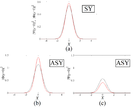
Figure 1: (Color online) (a) The cross section of the 2D profile of a stable symmetric ground state with $(\kappa,N)=(0.4,1)$. (b,c) The same for a stable asymmetric ground state with $(\kappa,N)=(0.4,4)$. Red solid and black dashed curves designate numerical and VA results, respectively.

In a systematic form, the numerical results for the symmetric states are presented, along with the respective VA prediction, in terms of the relation between the total norm, $N$ [see Eq. (21)], and chemical potential, $\mu$, in Fig. 2(a). The VA prediction stays close to the numerical result when the nonlinearity is relatively weak [in particular, the symmetric states displayed in Fig. 1(a) for $N=1$ correspond to a very small discrepancy in Fig. 2(a)]. The discrepancy increases as the nonlinearity grows stronger, causing, as said above, the switch of the departure of the 2D wave function from the GS of the HO towards the Townes soliton. In the limit of $\mu\rightarrow-\infty$, the total norm approaches value $N_{\max}^{(S=0)}\approx 11.70$, which is twice the well-known norm of the Townes soliton, $N_{\mathrm{Townes}}\approx 5.85$, at which the critical collapse sets in Berge (an approximate variational prediction for it is $N_{\mathrm{Townes}}=2\pi$ Anderson ).

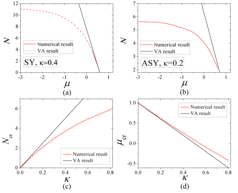
Figure 2: (Color online) Total norm $N$ versus chemical potential $\mu$ for (a) symmetric (“SY”) and (b) asymmetric (“ASY”) ground states (modes with $S=0$) in the 2D system, for indicated values of coupling constant $\kappa$. Red and black curves represent the numerical and variational results, respectively, see Eqs. (27) and (30). The dashed segment of the numerically generated $N(\mu)$ curve in (a) represents the branch destabilized by the SBB. (c) Critical values of total norm $N_{\mathrm{cr}}^{(S=0)}$ at the symmetry-breaking point of the GS in the 2D system, versus $\kappa$. (d) Critical values of the respective chemical potential, $\mu_{\mathrm{cr}}^{(S=0)}$, versus $\kappa$. Again, red and black curves represent, severally, numerical and VA results, see Eq. (32). The numerically found dependences displayed in (c) and (d) terminates at the point determined by Eq. (60).

A typical $N(\mu)$ dependence for the 2D asymmetric GS is displayed in Fig. 2(b), in which the numerically found and VA-predicted curves commence at the respective SBB points. In the limit of $\mu\rightarrow-\infty$, the total norm approaches the above-mentioned value $N_{\mathrm{Townes}}$, which asymptotically corresponds to the Townes soliton in component $\Phi_{S=0}$, while the contribution from $\Psi_{S=0}$ vanishes, as per Eq. (8). Note that, in both cases shown in Figs. 2(a) and (b), the $N(\mu)$ dependences satisfy the Vakhitov-Kolokolov criterion, $dN/d\mu<0$, which is the well-known necessary stability condition for modes supported by the self-focusing nonlinearity VK ; Berge .

Proceeding to detailed results for the stability of the symmetric and asymmetric 2D fundamental modes (alias GSs), we note that, as it might be expected, the asymmetric one is always stable when it exists (as the GS must be). The symmetric state loses its stability beyond the SBB point, i.e., at $N>N_{\mathrm{cr}}^{(S=0)}$, see Eq. (32). In direct simulations, it spontaneously transforms into an asymmetric state with residual oscillations, as shown in Fig. 3. Panels (c,d) in the figure demonstrate that an amplitude minimum in one oscillating component is attained simultaneously with the maximum in the other. This instability occurs in the region of $N_{\mathrm{cr}}^{(S=0)}<N<N_{\mathrm{Townes}}$. At $N>N_{\mathrm{Townes}}$, the 2D system suffers the onset of the collapse, as the spontaneous symmetry breaking makes the norm in one component much larger than in the other, allowing the larger norm to reach the collapse threshold for the single component, $N>N_{\mathrm{Townes}}$. As Fig. 4 demonstrates, the symmetry breaking accelerates in the course of the collapse development, driven by the growing nonlinearity strength in the collapsing component, while the mate component suffers depletion, rather than collapse.

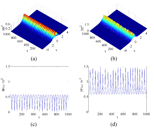
Figure 3: (Color online) (a,b) The numerically simulated evolution of an unstable 2D symmetric fundamental ($S=0$) state (shown is cross-section $y=0$) with $(\kappa,N)=(0.2,3)$, which demonstrates the onset of the spontaneous symmetry breaking with concomitant oscillations. (c,d) The respective evolution of densities of the two components at the center.

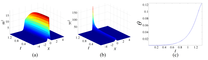
Figure 4: (Color online) (a,b) The evolution of an unstable symmetric fundamental soliton (shown is cross-section $y=0$) with $(\kappa,N)=(0.2,11.5)$, which demonstrates the acceleration of the symmetry breaking in the course of the development of the collapse. In panel (c), this is additionally illustrated by the dependence of asymmetry $\theta$ between the two components [see Eq. (10)] on time for the same solution.

The main objective of the analysis is the SBB in the two-component system. Basic results for the bifurcation acting on the 2D fundamental modes are presented in Fig. 5 in the form of relations between asymmetry $\theta$ [defined as per Eq. (10)] and total norm $N$. In agreement with the prediction of the VA, the corresponding SBB is of the supercritical type. The numerically found $\theta(N)$ curves terminate at the above-mentioned point of the onset of the critical collapse, $N=N_{\mathrm{Townes}}$.

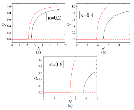
Figure 5: (Color online) Bifurcation diagrams, in the $(N,\theta)$ plane, for the fundamental modes (ground states) with $S=0$, at different values of the linear coupling constant: (a) $\kappa=0.2$, (b) $\kappa=0.4$, and (c) $\kappa=0.6$. Here, black and continuous/dashed red curves represent the variational results, and numerically found stable/unstable solutions, respectively.

With the increase of the coupling constant, $\kappa$, larger values of $N$ are required to for the onset of the symmetry breaking, therefore the accuracy of the VA prediction for the SBB deteriorates at large $\kappa$. It is relevant to stress that the SBB takes place in a finite interval of the values of the coupling constant, $0<\kappa\leq\kappa_{\max}$, with $\kappa_{\max}$ determined by the condition that the symmetry breaking occurs at $N=N_{\mathrm{Townes}}$, i.e., by equation

$$N_{\mathrm{cr}}^{(S=0)}\left(\kappa_{\max}\right)=N_{\mathrm{Townes}}$$ (59)

(at $\kappa>\kappa_{\max}$, the critical collapse occurs prior to the expected onset of the SBB). The respective numerical result is

$$\kappa_{\max}^{(S=0)}\approx 0.8.$$ (60)

It determines the termination points of the numerically found dependences $N_{{\rm cr}}(\kappa)$ and $\mu_{{\rm cr}}(\kappa)$ in Figs. 2(c,d).

IV.1.2 Symmetric and asymmetric vortices with $S=1$

Like GS, solutions of symmetric and asymmetric vortices are also produced by means of imaginary-time-integration method. Typical examples of shapes of stable symmetric vortices are shown in Figs. 6(a) and (b,c), respectively. Relations between total norm and chemical potential for families of vortices are displayed in Fig. 7, which shows that the stability regions of the symmetric and asymmetric vortices expand and shrink, respectively, with the increase of coupling constant $\kappa$. To explain these findings, we note, first, that in the decoupled limit, $\kappa=0$, the stability region for the vortices was known previously Dum :

$$0\leq N\leq N_{\mathrm{cr}}^{(S=1)}\left(\kappa=0\right)\approx 15.6,$$ (61)

which coincides with the stability boundary in Fig. 7(a) for $\kappa=0$ (it is multiplied by $2$ in comparison with Ref. Dum , where the boundary was given for the single component).

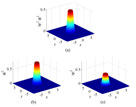
Figure 6: (Color online) (a) A stable symmetric vortex with $S=1$ and $(\kappa,N)=(0.4,8)$. (b,c) Two components of a stable asymmetric vortex with $(\kappa,N)=(0.4,8.8)$.

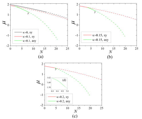
Figure 7: (Color online) Total norm $N$ versus chemical potential $\mu$ for symmetric and asymmetric vortices with $S=1$, at indicated values of the coupling constant, (a) $\kappa=0.1$, (b) $\kappa=0.15$, (c) $\kappa=0.2$. The decoupled system with $\kappa=0$ is included in (a) too, for the completeness’ sake. Inset (d) is a zoom of a small stability region which exists in (c). Solid and dashed lines designate stable and unstable branches, respectively. Arrows indicate points where the asymmetric vortices loose their stability. They are $N_{\max}^{(S=1)}$ for the asymmetric ones, see Eq. (64).

Next, the symmetric vortices in the coupled system feature the SBB at the respective critical value of the norm, $N_{\mathrm{cr}}^{(S=1)}(\kappa)$ [the $N(\mu)$ curves for the asymmetric vortices in Fig. 7(b) for each $\kappa$ originate precisely at $N=N_{\mathrm{cr}}^{(S=1)}(\kappa)$]. The numerically found dependence $N_{\mathrm{cr}}^{(S=1)}(\kappa)$ is displayed in Fig. 8, along with the respective dependence on $\kappa$ of the chemical potential at the SBB point. They can be empirically fitted by linear relations,

$$N_{\mathrm{cr}}^{(S=1)}(\kappa)=0.57+19.06\kappa,~{}\mu_{\mathrm{cr}}^{(S=1)}(\kappa)=2-1.86\kappa.$$ (62)

In fact, such linear dependences can be derived from the VA for the vortices [cf. similar relations (32) predicted by the VA for the modes with $S=0$]. We do not present this extension of the VA here in detail, as it is rather cumbersome.

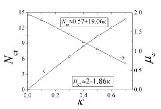
Figure 8: (Color online) The critical value of the total norm at the symmetry-breaking point, $N_{\mathrm{cr}}^{(S=1)}$, versus the coupling constant, $\kappa$, for vortices with $S=1$, corresponds to the black line with circles. The chemical potential at the bifurcation point, $\mu_{\mathrm{cr}}^{(S=1)}$, versus the coupling constant $\kappa$, is shown by the black line with triangles. As indicated in the figure, these dependences can be fitted by linear relations (62). They terminate at the point given by Eq. (63).

With the further increase of $\kappa$, the value $N_{\mathrm{cr}}^{(S=1)}(\kappa)$ attains the above-mentioned stability limit for the decoupled system, given by Eq. (61). As follows from Eq. (62), this happens at

$$\kappa=\kappa_{\max}^{(S=1)}\allowbreak\approx 0.81,$$ (63)

which is, interestingly, virtually the same as its counterpart for the modes with $S=0$, given by Eq. (60). Accordingly, dependences $N_{\mathrm{cr}}^{(S=1)}(\kappa)$ and $\mu_{\mathrm{cr}}^{(S=1)}(\kappa)$, displayed in Fig. 8, terminate close to $\kappa=\kappa_{\max}^{(S=1)}$. At $\kappa>\kappa_{\max}^{(S=1)}$, no stable asymmetric vortices exist, as the symmetric ones become unstable prior to the onset of the SBB. This fact explains the shrinkage of the stability region for the asymmetric vortices with the increase of $\kappa$, as observed in Fig. 7 and 13.

The SBB for vortices is illustrated by curves $\theta(N)$ which are displayed, for different values of $\kappa$, in Fig. 9, cf. similar diagrams for the models with $S=0$ in Fig. 5. These diagrams clearly demonstrate that the the SBB for the vortices is also of the supercritical type.

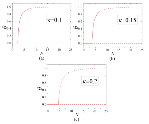
Figure 9: (Color online) Bifurcation diagrams, in the $(N,\theta)$ plane, for the vortices with $S=1$ at different values of the linear coupling constant: (a) $\kappa=0.1$, (b) $\kappa=0.15$, and (c) $\kappa=0.2$. Stable and unstable branches are shown by solid and dashed lines, respectively.

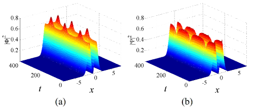
Figure 10: (Color online) The evolution of an unstable 2D symmetric ($S=1$) vortex (shown is cross-section $y=0$) with $(\kappa,N)=(0.4,8.8)$, which demonstrates the onset of the spontaneously symmetry breaking with residual oscillations.

Symmetric vortices destabilized by the SBB spontaneously transform into asymmetric ones with residual oscillations(see Fig. 10), similar to the spontaneous transition from unstable symmetric states with $S=0$ to oscillating asymmetric modes, as shown above in Fig. 3. Stable asymmetric vortices exist in the interval of $N_{\mathrm{cr}}^{(S=1)}<N<N_{\max}^{(S=1)}$, where $N_{\max}^{(S=1)}$ is the largest norm up to which asymmetric vortices remain stable, as shown in Fig. 7:

$$N_{\max}^{(S=1)}(\kappa=0.1)\approx 7.9,~{}N_{\max}^{(S=1)}(\kappa=0.15)\approx 6.9,~{}N_{\max}^{(S=1)}(\kappa=0.2)\approx 4.9.$$ (64)

At $N>N_{\max}^{(S=1)}$, two generic instability scenarios are possible, starting from the symmetric input. One (splitting)is shown in Fig. 11, which demonstrates that the evolution of symmetric vortices combines the spontaneous symmetry breaking between the $\phi$ and $\psi$ components and splitting of the vortex ring in two fragments, followed by the collapse of the fragments in the component carrying a larger amplitude (it is $\psi$, in Fig. 11; the asymmetric collapse may be compared to that displayed in Fig. 4 for the modes with $S=0$). The second scenario (crescent instability)is illustrated by Fig. 12: the asymmetric vortex rings spontaneously transforms into a crescent, which is followed by recovery of the ring. After several cycles of such transformations, the crescent’s component with a larger amplitude tends to evolve into an approximately fundamental state, while the component with a smaller norm develops a chaotic pattern. The former component will eventually suffer collapse, if the norm of the emergent fundamental state exceeds the value corresponding to the collapse onset. A similar scenario of the instability development of vortices in single-component self-attractive BEC was reported in Ref. HSaito .

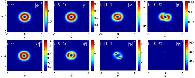
Figure 11: (Color online) Numerically simulated evolution of an unstable symmetric vortex with $S=1$ and $(\kappa,N)=(0.8,18)$, initiated by random noise (at the amplitude level of $5\%$) added to the input. This is a typical example of the splitting instability.

Figure 12: (Color online) Numerically simulated evolution of an unstable asymmetric vortex with $S=1$ and $(\kappa,N)=(0.2,6)$, initiated by random noise (at the amplitude level of $5\%$) added to the input. This figure presents a typical example of the crescent instability (see the main text).

In the single-component model, simulations of the evolution of the vortex with $S=1$ reveal a robust dynamical regime intermediate between the stability and the splitting followed by the collapse: in the interval of the norm which, in the present notation, is

$$15.56<N<20,$$ (65)

the vortex ring recurrently splits into two fragments that recombine back into the ring Dum ; HSaito . In the present system, systematic simulations demonstrate that such a stable regime does not occur at values of the coupling constant $0<\kappa\leq 0.81$, as the symmetry breaking destabilizes the fragments after the first splitting (approximately in the same fashion as shown in Fig. 11). At $\kappa\geq 4.35$, the linear coupling is so strong that the dynamics of the two-component system is identical to that of its single-component counterpart, hence stable splitting-recombination cycles, symmetric with respect to the $\phi$ and $\psi$ components, take place in interval (65). In the case of $0.81<\kappa<4.35$, the splitting-recombination regime is stable below the boundary in the $\left(\kappa,N\right)$ plane, which is shown by the dashed line in Fig. 13(a).

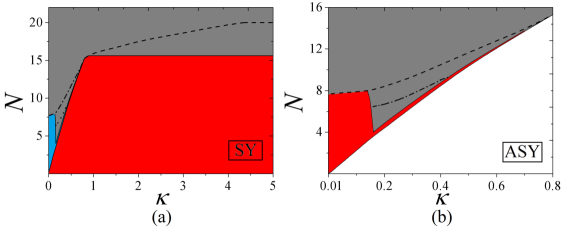
Figure 13: (Color online) The stability diagram for symmetric (a) and asymmetric (b) vortices with $S=1$ in the plane of $(\kappa,N)$. The red and gray colors designate, respectively, stability and instability areas. In panel (a), the small blue area represents instability with residual oscillations, while the gray area below the dashed-dotted curve designates the crescent instability similar to that shown in Fig. 12. Above the dotted line, this instability leads to the collapse of the component with the larger norm, but the collapse does not happen in the small gray sub-area below the dotted line. The gray area above the dashed-dotted and dashed lines represents the splitting instability scenario displayed in Fig. 11, while robust recurrent splitting-recombination cycles take place in the gray area below the dashed curve. In panel (b), the gray area under the dashed-dotted line represents the instability shown in Fig. 12, while in the area between the dashed and dashed-dotted lines instability similar to that in Fig. 12 occurs, finally leading to the collapse. Finally, the gray area above the dashed curve represents instability similar to that displayed in Fig. 11.

IV.2 The one-dimensional system

The VA for the 1D system, based on Eqs. (34) and (40), (43), predicts stable symmetric GS and dipole modes in a virtually exact form, see typical examples in Fig. 14(a,b). Above the SBB point, unstable symmetric GSs spontaneously transform into asymmetric counterparts with residual oscillations, as shown in Fig. 14(c,d), cf. the similar transition in the 2D system, displayed above in Fig. 3. The asymmetric GSs are completely stable in their existence region.

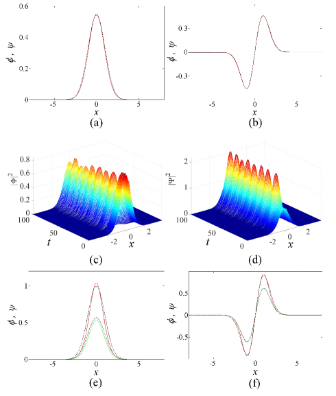
Figure 14: (Color online) (a,b) Typical examples of stable symmetric solutions for the 1D ground-state and dipole modes, with $(\kappa,N)=(0.4,1)$. Red solid and black dashed curves display the numerical and variational results, respectively. (c,d) The numerically simulated onset of the symmetry breaking in an unstable symmetric ground-state mode, with $(\kappa,N)=(0.4,2.5)$. Panels (e) and (f) display, severally, examples of stable asymmetric ground-state solutions, with $\left(\kappa,N\right)=(0.4,2)$, and dipole modes, with $\left(\kappa,N\right)=(0.4,2.7)$. Red and green solid curves represent two different components, as produced by the numerical solution, while black dashed lines depict their VA-predicted counterparts.

Systematic results for the 1D GS and dipole modes are reported by dint of $N(\mu)$ dependences in Fig. 15, and bifurcation diagrams in Figs. 16 and 17, respectively. In addition, critical values of the norm at which the symmetry-breaking transition takes place for both the GS and dipole modes are shown in Fig. 18. The figures also provide comparison of the VA predictions for these characteristics of the solution families with the numerical findings. In agreement with the VA result, the SBB in the 1D setting is of the supercritical type (on the contrary to the weakly subcritical SBB for free-space 1D solitons in the system of linearly coupled NLSEs bif1D ). Further, it is worthy to note that the accuracy of the VA, based on ansätze (34) and (48), is better for the dipole modes than for the GS. This is explained by the fact that the intrinsic structure of the dipoles makes them broader, hence their width is closer to that imposed by the trapping potential, as implied by the ansätze, than to the smaller soliton’s width determined by the self-trapping. Another noteworthy peculiarity revealed by Fig. 18 is that the critical norm is somewhat higher for the dipoles than for the GS. This fact too is explained by the effectively broader shape of the dipoles, which makes the nonlinearity somewhat weaker for them, in comparison with the GS mode.

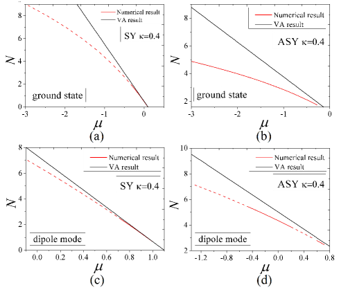
Figure 15: (Color online) Total norm $N$ versus chemical potential $\mu$ for symmetric (“SY”) (a) and asymmetric (“ASY”) (b) 1D ground state at $\kappa=0.4$. Red and black curves represent the numerical and variational results, the latter given by Eqs. (41)  and (44) for the symmetric and asymmetric states, respectively. (c,d) The same for the 1D dipole states, with the variational predictions given by Eqs. (52) and (55). Dashed are unstable segments of the numerically generated branches.

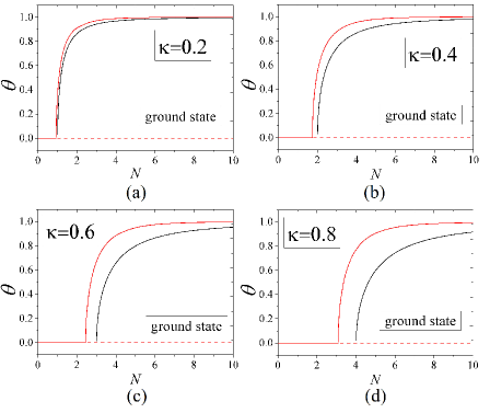
Figure 16: (Color online) Bifurcation diagrams, in the $(N,\theta)$ plane, for the 1D ground-state modes, at different values of the linear-coupling constant: (a) $\kappa=0.2$, (b) $\kappa=0.4$, (c) $\kappa=0.6$, and (d) $\kappa=0.8$. The red and black curves represent numerical findings and VA predictions, respectively.

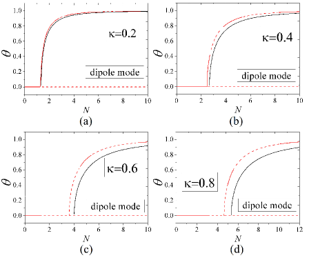
Figure 17: (Color online) The same as in Fig. 16, but for the 1D dipole modes.

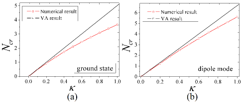
Figure 18: (Color online) (a) Critical values of total norm $N_{\mathrm{cr}}$, at which the 1D ground state undergoes the symmetry-breaking transition, versus coupling coefficient $\kappa$. (b) The same for the 1D dipole states. Again, red and black curves represent numerical and variational results, respectively [see Eqs. (46) and (58), as concerns the VA predictions].

When 1D symmetric dipole modes are destabilized by the SBB, at the respective critical points, $N=N_{\mathrm{cr}}^{\mathrm{(dip)}}$, they spontaneously transform into asymmetric counterparts, featuring residual oscillations (not shown here in detail), similar to the same transition for the GS, cf. Fig. 14(c,d). A more interesting finding, specific to the dipole mode, is that the branches of the asymmetric solutions, which are completely stable in the case of the 1D GSs, feature instability segments, with respective complex instability eigenvalues, corresponding to an oscillatory instability. As seen in Figs. 15(d) and 17, these segments are relatively narrow for small $\kappa$, essentially expanding at larger $\kappa$. In particular, at $\kappa=0.2$ and $0.4$, the asymmetric dipole states remain stable, respectively, in intervals $N_{\mathrm{cr}}^{\mathrm{(dip)}}(\kappa=0.2)=1.24<N<2.9$ and $N_{\mathrm{cr}}^{\mathrm{(dip)}}(\kappa=0.4)=2.48<N<2.7$ [see Figs. 17(a,b)]. Furthermore, Figs. 17 (c,d) demonstrate that, at $\kappa=0.6$ and $0.8$, this instability expands to a part of the originally stable branches of the symmetric dipole modes below the SBB point. Direct simulations show, in Fig. 19, that this specific type of the instability of the asymmetric and symmetric dipole modes transforms them into robust chaotically oscillating states. This instability is not essentially related to the two-component structure of the system, as the emerging chaotic states seem effectively symmetric, with respect to the two components.

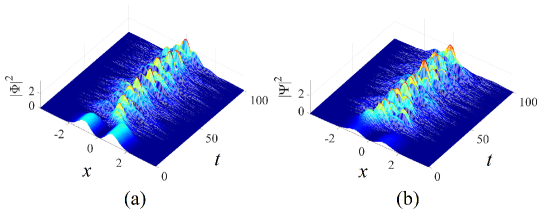
Figure 19: (Color online) The evolution of an unstable asymmetric dipole mode, with $(\kappa,N)=(0.6,4)$, which transforms into a spatially confined turbulent state.

V Conclusion

The objective of this work is to study manifestations of the spontaneously symmetry breaking of 2D fundamental modes and vortices, as well of 1D GS (ground state) and dipole mode (the first excited state), in the two-component model based on linearly coupled GPEs/NLSEs (Gross-Pitaevskii/nonlinear Schrödinger equations), with cubic self-attraction and the HO (harmonic-potential) trap. The system can be implemented in a two-layer BEC, and the 1D version also applies to dual-core optical waveguides. Although effects of the spontaneously symmetry breaking were studied, theoretically and experimentally, in many settings, these quite fundamental realizations were not considered before.

Families of 2D fundamental and vortical states, with vorticities $S=0$ and $S=1$, have been constructed by means of the variational and numerical methods, and their stability has been investigated by means of the computation of eigenvalues for small perturbations, and further verified in direct simulations. The respective SBB (symmetry-breaking bifurcation) is of the supercritical type (i.e., it represents a phase transition of the second kind) in all the cases. The asymmetric fundamental modes are completely stable, while asymmetric vortices keep their stability in rather narrow intervals of values of the norm, $N$, suffering the splitting into two fragments and subsequent collapse of the fragments at larger $N$, or featuring several cycles of transformations between the vortex ring and crescent, and eventually transforming into a fundamental state in one component, and a chaotic state in the other. The SBB occurs if the linear-coupling constant, $\kappa$, falls below a certain value $\kappa_{\max}\approx 0.81$, which is practically the same for the modes with $S=0$ and $S=1$. At $\kappa>\kappa_{\max}$, the strongly-coupled system behaves, essentially, as the single-component one; in particular, vortices demonstrate the regime of stable splitting-recombination cycles.

In 1D, families of GS and dipole solutions were found too in the variational and numerical forms. They also demonstrate the SBB of the supercritical type. The dipole modes are especially interesting, as, unlike the GSs and 2D vortices, they do not exist in the free space, and they are better approximated by the variational ansatz. A noteworthy feature of the asymmetric and symmetric dipoles is the appearance, with the increase of $\kappa$, of additional regions of oscillatory instability, unrelated to the spontaneous symmetry breaking. This instability transforms the dipoles into confined turbulent states.

A subject for continuation of the present analysis may be the study of Rabi oscillations between the two linearly components, in the 2D and 1D geometries alike, cf. Ref. double-well-BEC . It may also be interesting to consider a generalization for a system with a spinor (binary) wave function, which, in particular, may feature linear interconversion between spinor components inside each layer. In the latter context, the consideration of the spinor wave function subject to spin-orbit coupling SOC should be quite relevant. Lastly, it may be interesting too to introduce a $\mathcal{PT}$-symmetric version of the system PT , with equal amounts of linear gain and loss added to the two coupled equations, cf. Ref. Gena .

References

- (1) D. Landau and E. M. Lifshitz, Quantum Mechanics (Moscow: Nauka Publishers, 1974).
- (2) S. Giorgini, L. P. Pitaevskii, and S. Stringari, Rev. Mod. Phys. 80, 1215 (2008); H. T. C. Stoof, K. B. Gubbels, and D. B. M. Dickrsheid, Ultracold Quantum Fields (Springer: Dordrecht, 2009).
- (3) Y. S. Kivshar and G. P. Agrawal, Optical Solitons: From Fibers to Photonic Crystals (Academic Press: San Diego).
- (4) E. B. Davies, Symmetry breaking in a non-linear Schrödinger equation, Commun. Math. Phys. 64, 191-210 (1979); J. C. Eilbeck, P. S. Lomdahl, and A. C. Scott, The discrete self-trapping equation, Physica D 16, 318-338 (1985); A. W. Snyder, D. J. Mitchell, L. Poladian, D. R. Rowland, and Y. Chen, Physics of nonlinear fiber couplers, J. Opt. Soc. Am. B 8, 2101-2118 (1991).
- (5) E. M. Wright, G. I. Stegeman, and S. Wabnitz, Phys. Rev. A 40, Solitary-wave decay and symmetry-breaking instabilities in two-mode fibers, 4455-4466 (1989); C. Paré and M. Fłorjańczyk, Approximate model of soliton dynamics in all-optical couplers, ibid. 41, 6287-6295 (1990); A. I. Maimistov, Propagation of a light pulse in nonlinear tunnel-coupled optical waveguides, Kvant. Elektron. 18, 758-761 (1990) [Sov. J. Quantum Electron. 21, 687-690 (1991)]; P. L. Chu, B. A. Malomed, and G. D. Peng, Soliton switching and propagation in nonlinear fiber couplers: analytical results, J. Opt. Soc. Am. B 10, 1379-1385 (1993); N. Akhmediev and A. Ankiewicz, Novel soliton states and bifurcation phenomena in nonlinear fiber couplers, Phys. Rev. Lett. 70, 2395-2398 (1993); B. A. Malomed, I. M. Skinner, P. L. Chu, and G. D. Peng, Symmetric and asymmetric solitons in twin-core nonlinear optical fibers, Phys. Rev. E 53, 4084-4091 (1996); W. C. K. Mak, B. A. Malomed, and P. L. Chu, Solitary waves in coupled nonlinear waveguides with Bragg gratings, J. Opt. Soc. Am. B 15, 1685-1692 (1998); J. F. Jia, Y. P. Zhang, W. D. Li, and L. Li, Optical modes in a nonlinear double-channel waveguide, Opt. Commun. 283, 132-137 (2010); Y. Li, W. Pang, S. H. Fu, and B. A. Malomed, Two-component solitons with a spatially modulated linear coupling: Inverted photonic crystals and fused couplers, Phys. Rev. A 85, 053821 (2012); X. L. Shi, B. A. Malomed, F. W. Ye, X. F. Chen, Symmetric and asymmetric solitons in a nonlocal nonlinear coupler, ibid. 85, 053839 (2012); Y. Li, W. Pang, and B. A. Malomed, Nonlinear modes and symmetry breaking in rotating double-well potentials, Phys. Rev. A 86, 023832 (2012); D. A. Smirnova, A. V. Gorbach, I. V. Iorsh, I. V. Shadrivov, and Y. G. Kivshar, Nonlinear switching with a graphene coupler, Phys. Rev. B 88, 045443 (2013); M. J. Islam and J. Atai, Stability of gap solitons in dual-core Bragg gratings with cubic-quintic nonlinearity, Laser Phys. Lett. 12, 015401 (2015).
- (6) M. Matuszewski, B. A. Malomed, and M. Trippenbach, Spontaneous symmetry breaking of solitons trapped in a double-channel potential, Phys. Rev. A 75, 063621 (2007); H. Sakaguchi and B. A. Malomed, Symmetry breaking of solitons in two-component Gross-Pitaevskii equations, Phys. Rev. E 83, 036608 (2011).
- (7) G. J. Milburn, J. Corney, E. M. Wright, and D. F. Walls, Quantum dynamics of an atomic Bose-Einstein condensate in a double-well potential, Phys. Rev. A 55, 4318-4324 (1997); A. Smerzi, S. Fantoni, S. Giovanazzi, and S. R. Shenoy, Quantum coherent atomic tunneling between two trapped Bose-Einstein condensates, Phys. Rev. Lett. 79, 4950-4953 (1997); S. Raghavan, A. Smerzi, S. Fantoni, and S. R. Shenoy, Coherent oscillations between two weakly coupled Bose-Einstein condensates: Josephson effects, oscillations, and macroscopic quantum self-trapping, Phys. Rev. A 59, 620-633 (1999); L. Salasnich, A. Parola, and L. Reatto, Bose condensate in a double-well trap: ground state and elementary excitations, Phys. Rev. A 60, 4171-4174 (1999); M. Abad and A. Recati, A study of coherently coupled two-component Bose-Einstein condensates, Eur. Phys. J. D 67, 148 (2013).
- (8) G. Iooss and D. D. Joseph, Elementary Stability Bifurcation Theory (Springer-Verlag: New York, 1980).
- (9) T. Heil, I. Fischer, W. Elsässer, J. Mulet, and C. R. Mirasso, Chaos synchronization and spontaneous symmetry-breaking in symmetrically delay-coupled semiconductor lasers, Phys. Rev. Lett. 86, 795-798 (2001); C. Cambournac, T. Sylvestre, H. Maillotte, B. Vanderlinden, P. Kockaert, P. Emplit, and M. Haelterman, Symmetry-breaking instability of multimode vector solitons, Phys. Rev. Lett. 89, 083901 (2002); P. G. Kevrekidis, Z. Chen, B. A. Malomed, D. J. Frantzeskakis, and M. I. Weinstein, Spontaneous symmetry breaking in photonic lattices: Theory and experiment, Phys. Lett. A 340, 275-280 (2005); T. Kapitula, P. G. Kevrekidis, and Z. G. Chen, Three is a crowd: Solitary waves in photorefractive media with three potential wells, SIAM J. Appl. Dyn. Systems 5, 598-633 (2006); A. Guo, G. L. Salamo, D. Duchesne, R. Morandotti, M. Volatier-Ravat, V. Aimez, G. A. Siviloglou, and D. N. Christodoulides, Observation of -symmetry breaking in complex optical potentials, Phys. Rev. Lett. 103, 093902 (2009); Haddadi, A. M. Yacomotti, I. Sagnes, F. Raineri, G. Beaudoin, L. Le Gratiet, and J. A, Levenson, Photonic crystal coupled cavities with increased beaming and free space coupling efficiency, Appl. Phys. Lett. 102, 011107 (2013); F. Diebel, D. Leykam, M. Boguslawski, P. Rose, C. Denz, and A. Desyatnikov, All-optical switching in optically induced nonlinear waveguide couplers, Appl. Phys. Lett.. 104, 261111 (2014); P. Hamel, S. Haddadi, F. Raineri, P. Monnier, G. Beaudoin, I. Sagnes, A. Levenson, and A. M. Yacomotti, Spontaneous mirror-symmetry breaking in coupled photonic-crystal nanolasers, Nature Phot. 9, 311-315 (2015); A. Alberucci, A. Piccardi, N. Kravets, O. Buchnev, and G. Assanto, Soliton enhancement of spontaneous symmetry breaking, Optica 2, 783-789 (2015).
- (10) M. Albiez, R. Gati, J. Fölling, S. Hunsmann, M. Cristiani, and M. K. Oberthaler, Direct observation of tunneling and nonlinear self-trapping in a single bosonic Josephson junction, Phys. Rev. Lett. 95, 010402 (2005); A. Trenkwalder, G. Spagnolli, G. Semeghini, S. Coop, M. Landini, P. Castilho, L. Pezze, G. Modugno, M. Inguscio, A. Smerzi, and M. Fattori, Quantum phase transitions with parity-symmetry breaking and hysteresis, Nature Phys. 12, 826- 829 (2016).
- (11) M. Liu, D. A. Powell1, I. V. Shadrivov, M. Lapine, and Y. S. Kivshar, Spontaneous chiral symmetry breaking in metamaterials, Nature Comm. 5, 4441 (2014).
- (12) Spontaneous Symmetry Breaking, Self-Trapping, and Josephson Oscillations, ed. by B. A. Malomed (Springer-Verlag: Berlin and Heildelberg, 2013).
- (13) B. A. Malomed, Symmetry breaking in laser cavities, Nature Phot. 9, 287-289 (2015); B. A. Malomed, Spontaneous symmetry breaking in nonlinear systems: An overview and a simple model, in: Nonlinear Dynamics: Materials, Theory and Experiments (Springer Proceedings in Physics, vol. 173, 2016, ed. by M. Tlidi and M. Clerc), pp. 97-112.
- (14) N. Dror and B. A. Malomed, Symmetric and asymmetric solitons and vortices in linearly coupled two-dimensional waveguides with the cubic-quintic nonlinearity, Physica D 240, 526-541 (2011).
- (15) G. Burlak and B. A. Malomed, Stability boundary and collisions of two-dimensional solitons in -symmetric couplers with the cubic-quintic nonlinearity, Phys. Rev. E 88, 062904 (2013).
- (16) M. Quiroga-Teixeiro and H. Michinel, Stable azimuthal stationary state in quintic nonlinear optical media, J. Opt. Soc. Am. B 14, 2004-2009 (1997); M. L. Quiroga-Teixeiro, A. Berntson, and H. Michinel, Internal dynamics of nonlinear beams in their ground states: short- and long-lived excitation, J. Opt. Soc. Am. B 16, 1697-1704 (1997).
- (17) N. Jhajj, I. Larkin, E. W. Rosenthal, S. Zahedpour, J. K. Wahlstrand, and H. M. Milchberg, Spatiotemporal optical vortices, Phys. Rev. X 6, 031037 (2016).
- (18) A. Gubeskys and B. A. Malomed, Spontaneous soliton symmetry breaking in two-dimensional coupled Bose-Einstein condensates supported by optical lattices, Phys. Rev. A 76, 043623 (2007).
- (19) L. Salasnich and B. A. Malomed, Spontaneous symmetry breaking in linearly coupled disk-shaped Bose-Einstein condensates, Molecular Phys. 109, 2737-2745 (2011).
- (20) L. Salasnich, A. Parola, and L. Reatto, Effective wave equations for the dynamics of cigar-shaped and disk-shaped Bose condensates, Phys. Rev. A 65, 043614 (2002).
- (21) S. E. Pollack, D. Dries, M. Junker, Y. P. Chen, T. A. Corcovilos, and R. G. Hulet, Extreme Tunability of Interactions in a 7Li Bose-Einstein Condensate, Phys. Rev. Lett. 102, 090402 (2009).
- (22) F. Dalfovo and S. Stringari, Phys. Rev. A 53, 2477 (1996); R. J. Dodd, Approximate solutions of the nonlinear Schrödinger equation for ground and excited states of Bose-Einstein condensates, J. Res. Natl. Inst. Stand. Technol. 101, 545 (1996).
- (23) T. J. Alexander and L. Bergé, Phys. Rev. E 65, 026611 (2002); L. D. Carr and C. W. Clark, Phys. Rev. Lett. 97, 010403 (2006); D. Mihalache, D. Mazilu, B. A. Malomed, and F. Lederer, Vortex stability in nearly-two-dimensional Bose-Einstein condensates with attraction, Phys. Rev. A 73, 043615 (2006).
- (24) H. Saito and M. Ueda, Split instability of a vortex in an attractive Bose-Einstein condensate, Phys. Rev. Lett 89, 190402 (2002); H. Saito and M. Ueda, Split-merge cycle, fragmented collapse, and vortex disintegration in rotating Bose-Einstein condensates with attractive interactions, Phys. Rev. A 69, 013604 (2004).
- (25) L. Bergé, Phys. Rep. 303, 260 (1998); E. A. Kuznetsov and F. Dias, ibid. 507, 43 (2011); G. Fibich, The Nonlinear Schrödinger Equation: Singular Solutions and Optical Collapse (Springer: Heidelberg, 2015).
- (26) M. Desaix, D. Anderson, and M. Lisak, Variational approach to collapse of optical pulses, J. Opt. Soc. Am. B 8, 2082 (1991).
- (27) M. L. Chiofalo, S. Succi, and M. P. Tosi, Ground state of trapped interacting Bose-Einstein condensates by an explicit imaginary-time algorithm. Phys. Rev. E 62, 7438-7444 (2000).
- (28) N. G. Vakhitov and A. A. Kolokolov, Stationary solutions of the wave equations in a medium with nonlinearity saturation, Izv. Vyssh. Uchebn. Zaved. Radiofiz. 16, 1020-2028 (1973) [in Russian; English translation: Radiophys. Quantum Electron. 16,783-789 (1975)].
- (29) V. Galitski and I. B. Spielman, Spin-orbit coupling in quantum gases, Nature 494, 49-54 (2013); X. Zhou, Y. Li, Z. Cai, and C. Wu, Unconventional states of bosons with the synthetic spin-orbit coupling, J. Phys. B: At. Mol. Opt. Phys. 46, 134001 (2013); N. Goldman, G. Juzeliūnas, P. Öhberg, and I. B. Spielman, Light-induced gauge fields for ultracold atoms, Rep. Progr. Phys. 77, 126401 (2014); H. Zhai, Degenerate quantum gases with spin-orbit coupling: a review, Rep. Prog. Phys. 78, 026001 (2015). X. Jiang, Z. Fan, Z. Chen, W. Pang, Y. Li, and B. A. Malomed, Two-dimensional solitons in dipolar Bose-Einstein condensates with spin-orbit coupling, Phys. Rev. A 93, 023633 (2016); Y. Zhang, M. E. Mossman, T. Busch, P. Engels, C. Zhang, Properties of spin- orbit-coupled Bose-Einstein condensates, Front. Phys. 11, 118103 (2016).
- (30) R. El-Ganainy, K. G. Makris, D. N. Christodoulides, and Z. H. Musslimani, Theory of coupled optical -symmetric structures, Opt. Lett. 32, 2632-2634 (1007); Z. H. Musslimani, K. G. Makris, R. El-Ganainy, and D. N. Christodoulides, Optical solitons in periodic potentials, Phys. Rev. Lett. 100, 030402 (2008); S. V. Suchkov, A. A. Sukhorukov, J. Huang, S. V. Dmitriev, C. Lee, and Y. S. Kivshar, Nonlinear switching and solitons in -symmetric photonic systems, Laser Photonics Rev. 10, 177 (2016); V. V. Konotop, J. Yang, and D. A. Zezyulin, Nonlinear waves in -symmetric systems, Rev. Mod. Phys. 88, 035002 (2016).