Infinite mixing for one-dimensional maps with an indifferent fixed point

Abstract

We study the properties of ‘infinite-volume mixing’ for two classes of intermittent maps: expanding maps $[0,1]\longrightarrow[0,1]$ with an indifferent fixed point at 0 preserving an infinite, absolutely continuous measure, and expanding maps $\mathbb{R}^{+}\longrightarrow\mathbb{R}^{+}$ with an indifferent fixed point at $+\infty$ preserving the Lebesgue measure. All maps have full branches. While certain properties are easily adjudicated, the so-called global-local mixing, namely the decorrelation of a global and a local observable, is harder to prove. We do this for two subclasses of systems. The first subclass includes, among others, the Farey map. The second class includes the standard Pomeau-Manneville map $x\mapsto x+x^{2}$ mod 1. Morevoer, we use global-local mixing to prove certain limit theorems for our intermittent maps.

Mathematics Subject Classification (2010): 37A40, 37A25, 37E05, 37D25, 37C25.

1 Introduction

Expanding maps of the interval with indifferent, a.k.a. neutral, fixed points are among the most intensively studied classes of dynamical systems. They are considered the easiest examples of non-uniformly hyperbolic maps, where the mechanism that induces chaoticity is not as favorable—and somehow special—as in uniformly hyperbolic maps.

An indifferent fixed point can dramatically change the dynamical properties of an otherwise uniformly expanding map. Trajectories will spend long stretches of time in a neighborhood of the fixed point, nearly motionless, before returning to the strongly expanding region of the space, where they exhibit a seemingly random motion. In the physical literature, this behavior has been called intermittence, and maps with indifferent fixed points sometimes referred to as intermittent maps. They have been widely used as models for a variety of “anomalous” dynamical phenomena. A representative, far from exhaustive, list of references includes [GT, GNZ, BG, ZK, K].

If the fixed point is strongly neutral, which means that the second derivative is continuous there, these systems preserve a Lebesgue-absolutely continuous infinite measure under very general conditions [T1]. This and the fact that uniformly expanding interval maps are standard and somewhat elementary dynamical systems has led to intermittent maps of the interval being very popular in the field of infinite ergodic theory [T1, T2, A1, T3, Z, I1], considering also the many applications of its most notorious example, the Farey map [D, P, I2, KS, He, KMS].

Here we are interested in their mixing properties, especially in the sense of the recent definitions of infinite mixing given by Lenci [L1, L3]. The expression ‘infinite mixing’ refers to all the notions, or formal definitions, which are supposed to replace, or extend, the definition of mixing of finite ergodic theory.

The quest for an effective notion of infinite mixing has a long history (a short version of which may be found in the introduction of [L1]). Recent times have seen a significant surge of interest in this subject, both on its foundational aspects and on the application of new, sophisticated techniques to old problems [L1, DR, L2, MT1, Ko, A2, L3, Te, RT, LT, A3, MT2, L5, S, DN].

In [MT1, Te] Melbourne and Terhesiu studied a large class of interval maps with an indifferent fixed point, obtaining strong results related to the notion of mixing first envisaged by Hopf in 1937 [H] and later formalized, in slightly different ways, by Krickeberg [Kr], Papangelou [Pa] and Friedman [F]. This notion is sometimes referred to as Hopf-Krickeberg mixing or rational mixing. In the case of a map $T$ preserving an infinite measure $\mu$, it corresponds to the existence of a scaling rate $(\rho_{n})_{n\in\mathbb{N}}$ such that

$$\lim_{n\to\infty}\rho_{n}\,\mu((f\circ T^{n})g)=\mu(f)\mu(g),$$ (1.1)

for all $f,g$ in certain subspaces of $L^{1}(\mu)$. Here, as usual, $\mu(f)$ is short for $\int f\,d\mu$. (See also [A2] for the definition of rational weak mixing.)

From the point of view of the stochastic properties of dynamical systems, (1.1) corresponds to a local limit theorem. In the terminology used in the present paper, it represents a strong form of local-local mixing; cf. Section 2.2.

The definitions of infinite mixing introduced in [L1]—also referred to as infinite-volume mixing—hinge on the concept of a global observable. Informally speaking, a global observable is a bounded function that is supported more or less throughout the phase space, as opposed to a local observable, which is akin to a compactly supported function. In the present context, if $T:[0,1]\longrightarrow[0,1]$ has a neutral fixed point at 0 and preserves an infinite measure $\mu$ which assigns finite mass to all $[a,1]$, a global observable is any $F\in L^{\infty}(\mu)$ for which

$$\overline{\mu}(F):=\lim_{a\to 0^{+}}\frac{1}{\mu([a,1))}\int_{a}^{1}F\,d\mu$$ (1.2)

exists. In other words, a global observable is a bounded function $F$ whose averages over larger and larger portions of the space (in the sense of the measure) converge to an infinite-volume average $\overline{\mu}(F)$. A local observable is any $g\in L^{1}(\mu)$. (For the sake of readability, global and local observables are indicated, respectively, with uppercase and lowercase letters.)

We speak of global-global mixing when, for every pair of global observables $F,G$,

$$\lim_{n\to\infty}\overline{\mu}((F\circ T^{n})G)=\overline{\mu}(F)\overline{\mu}(G).$$ (1.3)

We call global-local mixing the case when, for all global observables $F$ and local observables $g$,

$$\lim_{n\to\infty}\mu((F\circ T^{n})g)=\overline{\mu}(F)\mu(g).$$ (1.4)

Both definitions have other versions as well, which are discussed in Section 2.2.

In [L1] global-global mixing and global-local mixing were proved, under suitable conditions, for dynamical systems representing random walks in $\mathbb{Z}^{d}$. In [L5] both types of mixing were verified for a certain class of uniformly expanding maps of the real line, the so-called quasi-lifts and their local modifications.

In this paper we show how maps with an indifferent fixed point of the type outlined earlier can never be global-global mixing, and present a general method to prove global-local mixing for such systems. The method covers a large class of examples, including the Farey map and many Pomeau-Manneville maps. It becomes particularly simple when, via conjugation, we represent our maps as dynamical systems on $\mathbb{R}^{+}$ preserving the Lebesgue measure.

To summarize, the various sections of the paper are organized as follows. Section 2 is the backbone: we describe in detail the classes of maps we study, review the notions of global and local observables, together with the various definitions of infinite mixing, and state our results. In Section 3 we present two examples of limit theorems that can be proved for intermittent maps that are global-local mixing. The rest of the paper is devoted to the proofs. In Section 4 we prove the simpler results. In Section 5 we give the scheme of the proof of global-local mixing. This is based on the existence of a local observable with certain monotonicity properties. Such existence will be established, for all cases considered, in Section 6. The proof of global-local mixing also uses the exactness of the map, which is a standard result. However, for the class of maps $\mathbb{R}^{+}\longrightarrow\mathbb{R}^{+}$ that we study, we found no proof in the literature, so we give our own proof in Appendix A. Finally, Appendix B contains the proofs of two technical results.

Acknowledgments. This research is part of the authors’ activity within the DinAmicI community, see www.dinamici.org. C. Bonanno and M. Lenci thank the Istituto Nazionale di Alta Matematica and its division Gruppo Nazionale di Fisica Matematica for various forms of support. P. Giulietti thanks the Universidade Federal do Rio Grande do Sul, Porto Alegre, Brazil, where part of this work was done. He also acknowledges the financial support of the Centro di Ricerca Matematica “Ennio de Giorgi” and of UniCredit Bank R&D Group, through the “Dynamics and Information Theory Institute” at the Scuola Normale Superiore.

2 Setup and results

In this section we give a detailed presentation of the maps we consider in the paper. We divide them in two classes: maps $[0,1]\longrightarrow[0,1]$ with a strongly neutral fixed point at 0, and maps $\mathbb{R}^{+}\longrightarrow\mathbb{R}^{+}$ with a neutral fixed point at $+\infty$ preserving the Lebesgue measure, cf. Figs. 1 and 2 later in the section. They are morally the same systems, because one can always pass from one type of map to the other via a suitable conjugation. But the conjugation will not map the first class exactly onto the second, hence the need to distinguish the two cases.

In order to emphasize the similar nature of the maps in the two classes, we choose to always use an open phase space. This means that for the rest the paper ‘unit interval’ will always indicate the open interval $(0,1)$. This choice has no consequence on our results.

2.1 Maps of the unit interval

In the case of a map $T:(0,1)\longrightarrow(0,1)$, we assume there to be a finite or infinite sequence of numbers $0=a_{0}<a_{1}<\ldots<a_{k}<\ldots\leq 1$. If the sequence is finite, its last element is $a_{N}:=1$; in this case we set $\mathcal{J}:=\{0,\ldots,N-1\}$. If the sequence is infinite, $\lim_{n}a_{n}=1$; in this case we set $\mathcal{J}=\mathbb{N}$ (in our notation $0\in\mathbb{N}$). For $j\in\mathcal{J}$, denote $I_{j}:=(a_{j},a_{j+1})$. Thus, $\mathscr{P}:=\{I_{j}\}_{j\in\mathcal{J}}$ is a partition of $(0,1)$ mod $m$, the Lebesgue measure on $\mathbb{R}$.

We assume that $T$ is a Markov map w.r.t. $\mathscr{P}$, with the following properties:

• $T|_{I_{j}}$ possesses an extension $\tau_{j}:[a_{j},a_{j+1}]\longrightarrow[0,1]$ which is bijective and $C^{2}$ up to the boundary.

• There exists $\Lambda>1$ such that $|\tau^{\prime}_{j}|\geq\Lambda$, for all $j\geq 1$.

• There exists $K>0$ such that $\displaystyle\frac{|\tau^{\prime\prime}_{j}|}{|\tau^{\prime}_{j}|^{2}}\leq K$, for all $j\geq 0$.

• $\tau_{0}$ is convex with $\tau_{0}(0)=0$, $\tau^{\prime}_{0}(0)=1$, and $\tau^{\prime}_{0}(x)>1$, for $x\in(0,a_{1}]$.

The following statements, which were proved, respectively, in [T1] and [T2], will be useful in the remainder.

Theorem 2.1

Under the assumptions (A1)-(A4),

• $T$ preserves an infinite invariant measure $\mu$ which is absolutely continuous w.r.t. the Lebesgue measure $m$ and, up to multiplicative constants, is the unique absolutely continuous invariant measure. Moreover, the infinite density $h:=d\mu/dm$ is positive and unbounded only near 0.

• $T$ is conservative and exact (w.r.t. $m$ or $\mu$, which is the same).

We recall that $T$ is said to be exact when, denoted by $\mathscr{A}$ the $\sigma$-algebra of its reference space, the tail $\sigma$-algebra $\bigcap_{n\in\mathbb{N}}T^{-n}\mathscr{A}$ is trivial, i.e., it contains only null sets or complements of null sets.

Exactness is a strong mixing property which has the distinct advantage of being defined in the same way both in finite and infinite ergodic theory. Within the scope of the present paper, it has the additional merit of being a key ingredient for the proof of the global-local mixing (1.4).

2.2 Infinite mixing for maps of the unit interval

For $F\in L^{\infty}((0,1),\mu)$ and $a\in(0,1)$, denote

$$\mu_{[a,1)}(F) :=\frac{1}{\mu([a,1))}\int_{a}^{1}F\,d\mu;$$ (2.1)

$$\overline{\mu}(F) :=\lim_{a\to 0^{+}}\mu_{[a,1)}(F).$$ (2.2)

The limit (2.2) might not exist. When it does, we say that $F$ is a global observable and call $\overline{\mu}(F)$ the infinite-volume average of $F$. The space of all global observables is denoted by $\mathcal{G}$. In addition, we call any $f\in\mathcal{L}:=L^{1}((0,1),\mu)$ a local observable.

Remark 2.2

In the framework of [L1] and [L3] the definitions (2.1)-(2.2) correspond to choosing the exhaustive family $\mathscr{V}:=\left\{[a,1)\>\left|\>0<a<1\right.\!\right\}$. An exhaustive family is a collection of finite-measure sets that play the role of “large boxes” in a reference space. The generic element of $\mathscr{V}$ will also be denoted $V$. The limit $a\to 0^{+}$ is called the infinite-volume limit. In more suggestive notation we will also indicate it by $V\nearrow(0,1)$.

To visualize an example of a global observable, one can think of a bounded function of $(0,1)$ which oscillates around 0 in such a way that the limit in (2.2) exists. A more intuitive visualization of a global observables will be given in the Section 2.3, where the reference space is $\mathbb{R}^{+}$. Notice that a bounded function which has a limit at 0 is also a global observable, but a very insignificant one, because it is arbitrarily close to a constant in all but a tiny fraction of the space (in the sense of the measure). Unquestionably, any reasonable definition of mixing must be trivially verified on constant observables.

We briefly recall the definitions of ‘infinite-volume mixing’ presented in [L1, L3]. The dynamical system $((0,1),\mu,T)$ is called global-local mixing of type

(GLM1)

if, $\forall F\in\mathcal{G}$, $\forall g\in\mathcal{L}$ with $\displaystyle\mu(g)=0$, $\displaystyle\lim_{n\to\infty}\,\mu((F\circ T^{n})g)=0$;

(GLM2)

if, $\forall F\in\mathcal{G}$, $\forall g\in\mathcal{L}$, $\displaystyle\lim_{n\to\infty}\,\mu((F\circ T^{n})g)=\overline{\mu}(F)\mu(g)$;

(GLM3)

if, $\forall F\in\mathcal{G}$, $\displaystyle\lim_{n\to\infty}\,\sup_{g\in\mathcal{L}\setminus 0}\frac{\left|\mu((F\circ T^{n})g)-\overline{\mu}(F)\mu(g)\right|}{\mu(|g|)}=0$.

It is called called global-global mixing of type

(GGM1)

if, $\forall F,G\in\mathcal{G}$, $\displaystyle\lim_{n\to\infty}\,\overline{\mu}((F\circ T^{n})G)=\overline{\mu}(F)\,\overline{\mu}(G)$;

(GGM2)

if, $\forall F,G\in\mathcal{G}$, $\displaystyle\lim_{{V\nearrow(0,1)}\atop{n\to\infty}}\mu_{V}((F\circ T^{n})G)=\overline{\mu}(F)\,\overline{\mu}(G)$.

The limit in (GGM2) means that, for all $\varepsilon>0$, there exists $M>0$ such that the l.h.s., defined as in (2.1), is $\varepsilon$-close to the limit for all $V=[a,1)$, with $\mu(V)\geq M$, and all $n\geq M$. It is called the ‘joint infinite-volume and time limit’; cf. [L3, Defn. 2.2].

Our first proposition states that if $T$ is such that (A1)-(A4) are satisfied, then $\overline{\mu}$ is an invariant functional for the dynamics. If this were not the case, the above definitions would not make sense. To keep the exposition fluid, we postpone the proof to Section 4.

Proposition 2.3

Let $T:(0,1)\longrightarrow(0,1)$ verify (A1)-(A4). For all $F\in\mathcal{G}$ and $n\in\mathbb{N}$, $\overline{\mu}(F\circ T^{n})$ exists and equals $\overline{\mu}(F)$.

Finally, the system is called local-local mixing

(LLM)

if, $\forall f\in\mathcal{L}\cap\mathcal{G}$, $g\in\mathcal{L}$, $\displaystyle\lim_{n\to\infty}\,\mu((f\circ T^{n})g)=0$.

Since, in the present case, $\mathcal{G}$ comprises all $F\in L^{\infty}$ which possess an infinite-volume average and $\mathcal{L}=L^{1}$, one verifies that (LLM) is equivalent to the definition of zero-type dynamical system: $\lim_{n\to\infty}\mu(T^{-n}A\cap A)=0$, for all $A$ with $\mu(A)<\infty$ [HK, DS].

The property with which we are most concerned in this article is (GLM2), which can be recast like this: For every $\mu$-absolutely continuous probability measure $\nu$ and every global observable $F$,

$$\lim_{n\to\infty}T^{n}_{*}\nu(F)=\overline{\mu}(F),$$ (2.3)

where $T^{n}_{*}\nu=\nu\circ T^{-n}$ denotes the push-forward of $\nu$ via the map $T^{n}$. In this sense, (GLM2) represents a very weak form of convergence of $T^{n}_{*}\nu$ to $\mu$, which cannot occur in any conventional sense, as the former are probability measures and the latter is an infinite measure.

For all the other properties we have the following.

Proposition 2.4

A map $T:(0,1)\longrightarrow(0,1)$ verifying (A1)-(A4) is (GLM1) and (LLM), but not (GLM3), (GGM1) or (GGM2).

Once again, we give the proof of Proposition 2.4 in Section 4. We will see that, in the present case, it is relatively easy to check all of the conditions except (GLM2). This does not mean, however, that these definitions are unimportant or give no information about the system; quite the contrary. For example, the fact that $T$ cannot be global-global mixing formalizes the idea that an expanding map with an indifferent fixed point has radically different chaotic properties than a uniformly expanding map. This is no surprise, given that the former is very close to the identity in the overwhelming majority of the space (in terms of the measure). By way of comparison, we observe that the uniformly expanding maps on $\mathbb{R}$ studied in [L5] are generally expected to be global-global mixing. (For further comparison with the results of [L5] see the last paragraph of Section 5.)

We now introduce a class of maps satisfying (A1)-(A4) which verify (GLM2). They are Markov maps with $N=2$ surjective branches. (The case $2<N<\infty$ can be treated as well, though the necessary hypotheses become more cumbersome, cf. Remark 2.8 below.)

In view of (A1), let us denote $\phi_{0}:=\tau_{0}^{-1}:[0,1]\longrightarrow[0,a_{1}]$ and $\phi_{1}:=\tau_{1}^{-1}:[0,1]\longrightarrow[a_{1},1]$. These functions, which extend the inverse branches of $T$, are bijective and $C^{2}$ up to the boundary. Moreover, $\phi_{0}^{\prime}(0)=1$, $\phi_{0}^{\prime}(x)\in(0,1)$ for $x\in(0,1]$, and $\phi_{0}$ is concave. Recalling that $h$ is the density of the infinite invariant measure $\mu$ given by Theorem 2.1(a), we make the following extra assumptions:

• $\phi_{1}$ is decreasing (equivalently, $\tau_{1}$ is decreasing).

• $\phi_{0}+\phi_{1}$ is increasing and concave.

• $\phi^{\prime}_{0}\,(h\circ\phi_{0})/h$ is differentiable, strictly decreasing and convex.

• $\phi_{0}^{\prime}\,(h\circ\phi_{0})+\phi_{1}^{\prime}\,(h\circ\phi_{1})\geq 0$.

Remark 2.5

If $h$ is decreasing, (A8) follows from (A6). In fact, $h>0$, $\phi^{\prime}_{0}>0$ and $\phi_{0}\leq\phi_{1}$ imply $\phi_{0}^{\prime}\,(h\circ\phi_{0})\geq\phi_{0}^{\prime}\,(h\circ\phi_{1})\geq-\phi_{1}^{\prime}\,(h\circ\phi_{1})$.

Theorem 2.6

Let $T:(0,1)\longrightarrow(0,1)$ satisfy assumptions (A1)-(A8) w.r.t. $\mathscr{P}=\{I_{0},I_{1}\}$. Then $T$ is (GLM2).

The proof of this theorem is given in Sections 5 and 6. An interesting family of maps which satisfy the hypotheses of the theorem is constructed starting from the Farey map:

$$T_{0}(x)=\left\{\begin{array}[]{ll}\displaystyle\frac{x}{1-x}\,,&x\in\left[0,\frac{1}{2}\right];\\[14.0pt] \displaystyle\frac{1-x}{x}\,,&x\in\left[\frac{1}{2},1\right].\end{array}\right.$$ (2.4)

It is well known that $T_{0}$ preserves the infinite measure on $(0,1)$ whose density is $h(x)=1/x$. The inverse branches of $T_{0}$ are easily computed to be $\phi_{0}(x)=x/(1+x)$ and $\phi_{1}(x)=1/(1+x)$.

For $\alpha\in(0,1)$, set $I_{0}:=(0,2^{\alpha-1})$ and $I_{1}:=(2^{\alpha-1},1)$, and consider the map $T_{\alpha}:(0,1)\longrightarrow(0,1)$ implicitly defined by the inverse branches

$$\phi_{0}(x):=\frac{x}{(1+x)^{1-\alpha}},\qquad\phi_{1}(x):=\frac{1}{(1+x)^{1-\alpha}},$$ (2.5)

where $\phi_{j}:I_{j}\longrightarrow[0,1]$, for $j\in\{0,1\}$. An example is shown in Fig. 1. We have

$$\phi^{\prime}_{0}(x)=\frac{1+\alpha x}{(1+x)^{2-\alpha}},\qquad\phi^{\prime}_{1}(x)=-\frac{1-\alpha}{(1+x)^{2-\alpha}}$$ (2.6)

and

$$\phi^{\prime\prime}_{0}(x)=-(1-\alpha)\,\frac{2+\alpha x}{(1+x)^{3-\alpha}},\qquad\phi^{\prime\prime}_{1}(x)=\frac{(2-\alpha)(1-\alpha)}{(1+x)^{3-\alpha}}.$$ (2.7)

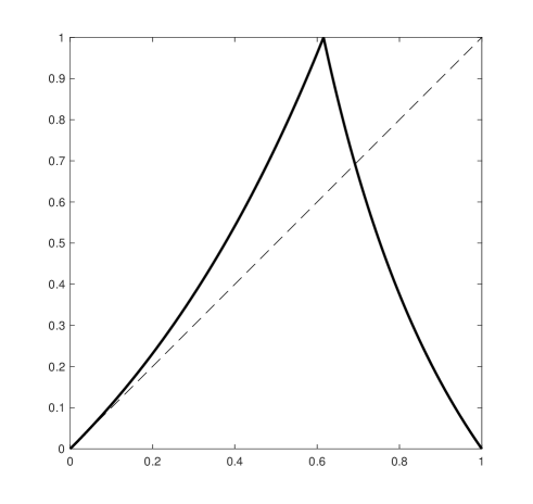
Figure 1: The map $T_{\alpha}$ defined in Section 2.2, for $\alpha=0.3$.

It is easy to check that $T_{\alpha}$ verifies (A1)-(A6). Moreover, $T_{\alpha}$ preserves the same measure preserved by the Farey map $T_{0}$. In fact, given $h(x)=1/x$, one has

$$|\phi^{\prime}_{0}|\,(h\circ\phi_{0})+|\phi^{\prime}_{1}|\,(h\circ\phi_{1})=h,$$ (2.8)

which implies that $\int(F\circ T_{\alpha})h\,dm=\int F\,h\,dm$, for all $F\in L^{\infty}$. (In other words, if $P$ denotes the transfer operator of $T_{\alpha}$ relative to $\mu$, cf. (6.1), the identity (2.8) is equivalent to $P1=1$, where $1$ is the (non-integrable) function which is identically equal to 1.) Finally, the equation

$$\phi^{\prime}_{0}(x)\,\frac{h(\phi_{0}(x))}{h(x)}=\frac{1+\alpha x}{(1+x)},$$ (2.9)

proves (A7), while (A8) follows from (A6) and the monotonicity of $h$, as pointed out in Remark 2.5.

Remark 2.7

Since the parameter $\alpha$ ranges in $(0,1)$, the above family does not include the Farey map (2.4). The problem is that $T_{0}^{\prime}(1)=-1$ and (A2) is not verified. But the conclusions of Theorem 2.6 hold for the Farey map too. As it will be clear later, cf.  Definition 5.1 and Theorem 5.2, it is sufficient to find a persistently monotonic local observable for $T_{0}$. This was done in [I2, Lem 8.13].

Remark 2.8

Theorem 2.6 can be extended to the case of $N$ branches, $2<N<\infty$, if, in addition to (A1)-(A4), the following assumptions are made:

• $\tau_{k}$ is increasing and convex for all $k\in\{0,\dots,N-2\}$; $\tau_{N-1}$ is decreasing.

• $\sum_{k=0}^{N-1}\phi_{k}$ is increasing and concave.

• $\phi^{\prime}_{k}\,(h\circ\phi_{k})/h$ is strictly decreasing and convex for all $k\in\{0,\dots,N-2\}$.

• $h$ is decreasing (or the analogue of (A8) holds with $\phi_{k}$ in place of $\phi_{0}$, for all $k\in\{0,\dots,N-2\}$).

The proof of this generalization adds computations but no new ideas to the one presented in the paper, so we omit it.

A very popular family of intermittent maps of the unit interval is the loosely defined class that goes by the names of Pomeau and Manneville. These maps have been introduced to study in full rigor certain intermittency phenomena initially described by Pomeau and Manneville in the 1980’s [PM, M]. Although no precise definition exists, most mathematicians would agree that a Pomeau-Manneville map is a map of $(0,1)$ with two increasing branches satisfying at least (A1) and (A4). It is natural to ask weather maps of this type are global-local mixing. Neither Theorem 2.6 nor Remark 2.8 address this case because they assume one branch to be decreasing. Nonetheless, many Pomeau-Manneville maps are (GLM2). For a given system, this can be shown via the results of Section 2.4 below, provided one has enough information about the invariant measure $\mu$. The problem, however, is that the general theorems that are available at this time [T1, T4] do not provide enough control on $\mu$. We refer the reader to Remarks 2.15 and 2.16 in Section 2.4.

2.3 Maps of the half-line

Given a map $T:\mathbb{R}^{+}\longrightarrow\mathbb{R}^{+}$, we assume that there exists a finite or infinite sequence $a_{1}>a_{2}>\ldots>a_{k}>\ldots\geq 0$. If the sequence is finite, its last element is $a_{N}:=0$; in this case $\mathcal{J}:=\{0,\ldots,N-1\}$. If the sequence is infinite, $\lim_{n}a_{n}=0$; in this case $\mathcal{J}=\mathbb{N}$. Denote $I_{0}:=(a_{1},+\infty)$ and, for $j\in\mathcal{J}\setminus\{0\}$, $I_{j}:=(a_{j+1},a_{j})$. Once again, $\mathscr{P}:=\{I_{j}\}_{j\in\mathcal{J}}$ is a partition of $\mathbb{R}^{+}$ mod $m$.

We also assume that:

• $T|_{I_{j}}$ is a bijective map onto $\mathbb{R}^{+}$, and possesses an extension $\tau_{j}$ which, for $j=0$, is defined on $[a_{1},+\infty)$ and, for $j\geq 1$, is defined on $[a_{j+1},a_{j})$ or $(a_{j+1},a_{j}]$. $\tau_{j}$ is $C^{2}$ up the boundary.

• There exists $\Lambda>1$ such that $|\tau^{\prime}_{j}|\geq\Lambda$, for all $j\geq 1$.

• There exists $K>0$ such that $\displaystyle\frac{|\tau^{\prime\prime}_{j}|}{|\tau^{\prime}_{j}|^{2}}\leq K$, for all $j\geq 0$.

• The function $u(x):=x-\tau_{0}(x)$ is positive, convex and vanishing (hence decreasing), as $x\to+\infty$. Furthermore, $u^{\prime\prime}$ is decreasing (hence vanishing).

• $T$ preserves the Lebesgue measure $m$.

The most restrictive assumption here, compared to Section 2.1, is (B5): we require $T$ to preserve not just an absolutely continuous measure, but exactly the Lebesgue measure. Some of the results we obtain (for example, Theorem 2.9 and Proposition 2.11) would also hold in the case where $T$ preserves an absolutely continuous, infinite, locally finite measure. With assumption (B5), however, the infinite-volume average of a global observable is defined in a very natural way, see (2.10).

Note that, given a $T_{o}:(0,1)\longrightarrow(0,1)$ satisfying (A1)-(A4), it is straightforward to find a conjugation $\Phi:(0,1)\longrightarrow\mathbb{R}^{+}$ such that $T:=\Phi\circ T_{o}\circ\Phi^{-1}$ verifies (B5). It suffices to take $\Phi(x):=\int_{x}^{1}h\,dm$, where $h$ is the Radon-Nikodym derivative mentioned in Theorem 2.1(a). But $T$ might not verify the other assumptions. For instance, it might not be expanding.

In analogy with Theorem 2.1(b), we have:

Theorem 2.9

Under assumptions (B1)-(B5), $T$ is conservative and exact.

The proof of Theorem 2.9—in fact, a generalization thereof—is given in Appendix A.

The observables that we associate with these types of maps are completely analogous to those defined in Section 2.2, with the difference that use $m$ instead of $\mu$. More precisely, the class of global observables is the space $\mathcal{G}$ of all $F\in L^{\infty}(\mathbb{R}^{+},m)$ such that

$$\exists\overline{m}(F):=\lim_{a\to+\infty}m_{(0,a]}(F):=\lim_{a\to+\infty}\frac{1}{a}\int_{0}^{a}F\,dm.$$ (2.10)

Correspondingly, the generic large box in reference space is $V=(0,a]$, and the infinite-volume limit, here denoted $V\nearrow\mathbb{R}^{+}$, is the limit $a\to+\infty$. Finally, the class of local observables is $\mathcal{L}:=L^{1}(\mathbb{R}^{+},m)$.

It is easy to see that any bounded periodic $F$ is a global observable, and $\overline{m}(F)$ is the average of $F$ over a period. Also, a large variety of “quasi-periodic” functions belong in $\mathcal{G}$, for instance $F(x):=e^{2\pi ix/\alpha}G(x)$, where $G$ is a bounded periodic function (in this case, if the ratio between $\alpha$ and the period of $G$ is irrational, $\overline{m}(F)=0$; otherwise $F$ is periodic). More “random” functions also belong in $\mathcal{G}$: for example, if $f:\mathbb{R}\longrightarrow\mathbb{C}$ is bounded and supported in $(0,b)$, and $(c_{k})_{k\in\mathbb{N}}$ is a bounded sequence which possesses a Cesaro average, then $F(x):=\sum_{k\in\mathbb{N}}c_{k}f(x-kb)$ is a global observable.

2.4 Infinite mixing for maps of the half line

For $T:\mathbb{R}^{+}\longrightarrow\mathbb{R}^{+}$ we consider the same definitions of infinite-volume mixing presented in Section 2.2, with the understanding that $\mathcal{G}$ and $\mathcal{L}$ are those defined earlier, $\mu$ is the Lebegue measure $m$, the exhaustive family is $\mathscr{V}:=\left\{(0,a]\>\left|\>a>0\right.\!\right\}$, and the infinite-volume limit is $V\nearrow\mathbb{R}^{+}$ or, in other words, $a\to+\infty$. The same results as in Section 2.2 hold here, and they are again proved in Section 4.

Proposition 2.10

Let $T:\mathbb{R}^{+}\longrightarrow\mathbb{R}^{+}$ verify (B1)-(B5). For all $F\in\mathcal{G}$ and $n\in\mathbb{N}$, $\overline{m}(F\circ T^{n})$ exists and equals $\overline{m}(F)$.

Proposition 2.11

A map $T:\mathbb{R}^{+}\longrightarrow\mathbb{R}^{+}$ verifying (B1)-(B5) is (GLM1) and (LLM), but not (GLM3), (GGM1) or (GGM2).

We now introduce a class of maps satisfying (B1)-(B5) which verify (GLM2). They will be determined by the extra assumption:

• $\tau_{j}$ is increasing and convex for all $j\geq 1$.

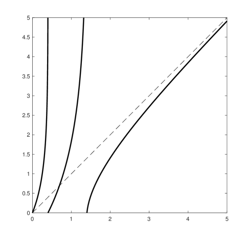
Figure 2: An example of a map $\mathbb{R}^{+}\longrightarrow\mathbb{R}^{+}$ verifying (B1)-(B6).

An example of such a map is shown in Fig. 2. Once again, let $\phi_{j}$ denote the inverse of $\tau_{j}$. By (B1) and (B4), the functions $\phi_{j}$ are bijective and $C^{2}$ up to the boundary, and $\phi_{0}$ is increasing and convex. By (B6), $\phi_{j}$ is increasing and concave for all $j\geq 1$.

Remark 2.12

If $T$ has only two branches, the convexity of $\tau_{1}$ is a consequence of the other hypotheses. In fact, cf. the proof of Theorem 6.3, the preservation of the Lebesgue measure reads $\phi_{0}^{\prime}+\phi_{1}^{\prime}=1$, whence $\phi_{0}^{\prime\prime}+\phi_{1}^{\prime\prime}=0$. Therefore $\phi_{0}$ and $\phi_{1}$ have opposite convexities. The same then holds for $\tau_{0}$ and $\tau_{1}$.

Theorem 2.13

Let $T:\mathbb{R}^{+}\longrightarrow\mathbb{R}^{+}$ satisfy assumptions (B1)-(B6). Then $T$ is (GLM2).

Remark 2.14

The above theorem can be improved to include maps $T:\mathbb{R}^{+}\longrightarrow\mathbb{R}^{+}$ which verify (B1)-(B5) and have two branches, with $\tau_{1}$ decreasing. In this case, however, we need to assume that the functions $\tau_{j}$ are $C^{3}$ up to the boundary, and add the following hypotheses:

• $\phi_{0}+\phi_{1}$ is increasing.

• $\phi^{\prime\prime}_{1}-(\phi^{\prime}_{1})^{2}>0$.

• For each $x\in\mathbb{R}^{+}$, one of the following two conditions holds: either

  $$\phi^{\prime\prime\prime}_{1}(x)+\phi^{\prime\prime}_{1}(x)>0\quad\text{and}\quad 3\phi^{\prime\prime}_{1}(x)-(\phi^{\prime}_{1}(x))^{2}+\phi^{\prime}_{1}(x)>0;$$

  or

  $$\phi^{\prime\prime\prime}_{1}(x)+\phi^{\prime\prime}_{1}(x)>(\phi^{\prime}_{1}(x))^{2}.$$

We omit the proof of this extension for the same reasons as in Remark 2.8. The interested reader can nevertheless find it in [BGL], where it is used to prove that the Boole map is (GLM2).

Remark 2.15

As discussed in Section 2.3, any map $T_{o}:(0,1)\longrightarrow(0,1)$ satisfying (A1)-(A4) can always be conjugated to a map $T:\mathbb{R}^{+}\longrightarrow\mathbb{R}^{+}$ that satisfies (B5), that is, preserves the Lebesgue measure. The conjugation is $T:=\Phi\circ T_{o}\circ\Phi^{-1}$, where $\Phi(x):=\int_{x}^{1}h\,dm$ and $h$ is an (infinite) invariant density for $T_{o}$. Therefore, with enough information about $h$, one will be able to check whether $T$ satisfies the hypotheses of Theorem 2.13, thus showing that $T$ and therefore $T_{o}$ are (GLM2). (Notice that all definitions of infinite-volume mixing are invariant w.r.t. the above conjugation.) For example, the Pomeau-Manneville map $T_{o}(x):=x+x^{2}$ mod 1 has an invariant density $h(x)=1/x+1/(1+x)$ [T4]. By construction, the corresponding $T$ has two increasing full branches, which are $C^{\infty}$ because $h$ is. It is a simple calculation to show that the branch $\tau_{0}$ is concave, implying (B6) via Remark 2.12. The hypotheses (B2)-(B4) are also satisfied. Actually, as it will be clear later on (cf. Theorems 5.2 and 6.3), (B2)-(B4) are not directly needed in the proof of global-local mixing: they are only used to show that $T$ is exact, which is another ingredient of the proof. But if one knows a priori that $T$ is exact, which in this case follows from the exactness of $T_{o}$ (Theorem 2.1(b)), one only need check condition (B6) for $T$. For a map $T_{o}$ with two increasing branches, by Remark 2.12, this amounts to checking that

$$T^{\prime}(x)=T_{o}^{\prime}(\Phi^{-1}(x))\,\frac{h(T_{o}(\Phi^{-1}(x)))}{h(\Phi^{-1}(x))}$$ (2.11)

is decreasing on the support of the branch $\tau_{0}$, i.e, for $x>a_{1}$. This is equivalent to

$$\log T^{\prime}(\Phi(x))=\log T_{o}^{\prime}(x)+\log h(T_{o}(x))-\log h(x)$$ (2.12)

being increasing for $0<x<a_{o1}$, where $a_{o1}:=\Phi^{-1}(a_{1})$ is the point of $(0,1)$ that separates the two Markov intervals of $T_{o}$.

Remark 2.16

The procedure that we have outlined in the previous remark can also be used in the opposite direction: starting from a map $T:\mathbb{R}^{+}\longrightarrow\mathbb{R}^{+}$ verifying (B1)-(B6), and therefore (GLM2), one can construct an endless number of global-local mixing maps $T_{o}:=\Phi^{-1}\circ T\circ\Phi:(0,1)\longrightarrow(0,1)$. This is in fact very easy, as assumptions (B1)-(B6) are rather general and one has ample freedom to choose $h$, and thus $\Phi$. For example, given a two-branched map $T$ satisfying (B1)-(B6), and chosen $h(x):=1/x^{p}$, with $p\geq 1$, simple computations show that $T_{o}$ has a strongly neutral fixed point at 0 and is expanding and convex in a neighborhood of 0. That $T_{o}$ has two full increasing branches and preserves $\mu$, with $h=d\mu/dm$, is obvious by construction. So $T_{o}$ is at least similar to a Pomeau-Manneville map. (In practice, most examples one will cook up lead to a fully convex branch at the origin.) This observation shows that one can construct many global-local mixing maps of the unit interval with any index $p\geq 1$; by this we mean here that the invariant density has a singularity of the type $x^{-p}$, as $x\to 0^{+}$. So it makes sense to study problems of linear response in this context as well—e.g., the response of $\overline{\mu}_{p}$ w.r.t. $p$ (see [BT, GG, BRS] and references therein for the corresponding problem in the finite-measure case, possibly with noise).

3 Applications

Before proving the results oulined in Section 2, we present two applications which show the usefulness of (GLM2) in deriving the statistical properties of intermittent maps preserving an infinite measure.

3.1 Equidistribution of hitting times in residue classes

Let $T:(0,1)\longrightarrow(0,1)$ be a map satisfying the assumptions of Theorem 2.6, or the Farey map, or any map of the same type for which (GLM2) holds; cf. Remarks 2.7 and 2.15.

In order to study the intermittent behavior of these maps in quantitative terms, one looks at how much time the typical orbit spends in a neighborhood of the fixed point. The choice of the neighborhood is not important, so one usually picks the Markov interval $I_{0}$. Thus, an observable of interest is the hitting time of a point $x\in(0,1)$ to $J:=(0,1)\setminus I_{0}=[a_{1},1)$:

$$H(x):=\min\left\{k\geq 0\>\left|\>T^{k}(x)\in J\right.\!\right\}.$$ (3.1)

It is clear that, with the exception of countably many points $x$, $H(T^{n}(x))$ is well-defined for all $n\in\mathbb{N}$. We denote by $\mathcal{M}$ the full-measure subset of $(0,1)$ where the $H\circ T^{n}$ is well-defined for all $n$.

Consider the level sets of $H$, i.e., $B_{k}:=\left\{x\in\mathcal{M}\>\left|\>H(x)=k\right.\!\right\}$, with $k\in\mathbb{N}$. They form a partition of $(0,1)$ (mod $m$) such that $B_{0}=J\cap\mathcal{M}$ and, for $k\geq 1$, $B_{k}\subset I_{0}$. Also for $k\geq 1$, $T|_{B_{k}}$ is a diffeomorphism $B_{k}\longrightarrow B_{k-1}$. Now, take $x\in\mathcal{M}$ and consider its itinerary $(\ell_{n})=(\ell_{n}(x))_{n\in\mathbb{N}}$ w.r.t. the partition $\{B_{k}\}_{k\in\mathbb{N}}$. This means that $T^{n}(x)\in B_{\ell_{n}}$, for all $n\in\mathbb{N}$. The expansivity of $T$ implies that the mapping $x\mapsto(\ell_{n})$ is injective, that is, equal itineraries correspond to equal points in $(0,1)$.

Remark 3.1

In the case of the Farey map, $\mathcal{M}=(0,1)\setminus\mathbb{Q}$ and

$$B_{k}=\left(\frac{1}{k+2},\frac{1}{k+1}\right)\setminus\mathbb{Q}.$$

The sets $C_{k}=B_{k-1}$ ($k\geq 1$) are sometimes called Farey cylinders. The itinerary $(\ell_{n})$ of a point $x\in(0,1)\setminus\mathbb{Q}$ is related to its continued fraction expansion $[a_{1},a_{2},a_{3},\ldots]$ as follows:

$$(\ell_{0},\ell_{1},\ell_{2},\ldots)=(a_{1}-1,a_{1}-2,\ldots,0,a_{2}-1,a_{2}-2,\ldots,0,a_{3}-1,\ldots).$$

Notice that, since $x$ is irrational, the expansion $[a_{1},a_{2},a_{3},\ldots]$ is infinite. (We ask the reader to forgive the abuse of notation whereby in the confines of this remark $a_{j}$ denotes a digit in the continued fraction expansion, while in the rest of the paper it denotes a point in $[0,1]$.)

Coming back to the general case, one can use the partition $\{B_{k}\}$ to construct global observables. Given $q\in\mathbb{Z}^{+}$ and $f_{j}\in\mathbb{C}$, for $0\leq j\leq q-1$, denote by $F:(0,1)\longrightarrow\mathbb{C}$ the step function defined ($m$-almost everywhere) by the relation:

$$F(x)=f_{j}\quad\Longleftrightarrow\quad x\in B_{k},\>\mbox{ with }k\equiv j\>(\mbox{mod }q).$$ (3.2)

Proposition 3.2

Any $F:(0,1)\longrightarrow\mathbb{C}$ defined as in (3.2) is a global observable with

$$\overline{\mu}(F)=\frac{1}{q}\sum_{j=0}^{q-1}f_{j}.$$

Proof. In Section B.1 of Appendix B.

An example of interest, given the discussion at the beginning of the section, is the global observable $H_{q}:(0,1)\longrightarrow\{0,1,\ldots,q-1\}$ given by $f_{j}=j$. The previous proposition shows that $\overline{\mu}(H_{q})=(q-1)/2$. Observe that, for all $x\in\mathcal{M}$ and $n\in\mathbb{N}$, $H_{q}(T^{n}(x))=\ell_{n}(x)\>(\mbox{mod }q)$.

We want to study the limiting distribution of $H_{q}\circ T^{n}$, seen as a random variable of $x\in\mathcal{M}$. For this we must specify a probability on $\mathcal{M}$. The invariant measure $\mu$ itself is not an option because it is infinite. However, since $\mu$ is the reference measure of the dynamical system, it is reasonable to use the probability measure $\mu_{g}$ defined by a certain density $g$ relative to $\mu$. In other words, given $g\in L^{1}((0,1),\mu)$, with $g\geq 0$ and $\mu(g)=1$, we consider the measure $\mu_{g}$ such that $d\mu_{g}/d\mu=g$. By Theorem 2.1(a), $\mu_{g}$ is absolutely continuous w.r.t. the Lebesgue measure on $(0,1)$, so it makes no difference to think of it as a measure on $(0,1)$ or $\mathcal{M}$.

It would be desirable for the limiting distribution not to depend on $g$. We adapt a definition found in [A1, §3.6].

Definition 3.3

Let $F_{n}$ be a sequence of measurable functions $(0,1)\longrightarrow\mathbb{R}$, and $X$ a random variable on some probability space $(\Omega,\mathbb{P})$. We say that $F_{n}$ converges to $X$ in strong distributional sense, as $n\to\infty$, if the distribution of $F_{n}$ w.r.t. $\mu_{g}$ converges to that of $X$, for all densities $g$. In other words, for all probability measures $\nu\ll\mu$ and all continuous bounded functions $\Psi:\mathbb{R}\longrightarrow\mathbb{R}$,

$$\lim_{n\to\infty}\int_{0}^{1}(\Psi\circ F_{n})\,d\nu=\int_{\Omega}(\Psi\circ X)\,d\mathbb{P}.$$

Proposition 3.4

As $n\to\infty$, $H_{q}\circ T^{n}$ converges in strong distributional sense to the uniform random variable on the set $\{0,1,\ldots,q-1\}$.

Proof. We achieve the result by showing the pointwise convergence of the corresponding characteristic functions.

The characteristic function of $H_{q}\circ T^{n}$, relative to $\mu_{g}$, is given by

$$\varphi_{n,g}(\theta):=\mu_{g}\!\left(e^{i\theta H_{q}\circ T^{n}}\right)=\mu\!\left(\left((e^{i\theta H_{q}})\circ T^{n}\right)g\right).$$ (3.3)

By Proposition 3.2, $e^{i\theta H_{q}}$ is a global observable with $\overline{\mu}(e^{i\theta H_{q}})=q^{-1}\sum_{j=0}^{q-1}e^{i\theta j}$. On the other hand, (GLM2) implies that, for all densities $g$,

$$\lim_{n\to\infty}\varphi_{n,g}(\theta)=\overline{\mu}(e^{i\theta H_{q}})\mu(g)=\frac{1}{q}\sum_{j=0}^{q-1}e^{i\theta j},$$ (3.4)

which is the characteristic function of the uniform random variable on the set $\{0,1,\ldots,q-1\}$. Q.E.D.

In view of the previous considerations, the above result gives a meaning, within the scope of infinite ergodic theory, to the phrase ‘losing memory of the initial conditions’. For all choices $\nu\ll\mu$ of the randomness of the initial conditions, the $n^{\mathrm{th}}$ hitting time $\ell_{n}$, when considered mod $q$, converges to the uniform random variable on $\{0,1,\ldots,q-1\}$, as $n\to\infty$. This is the “most random” behavior for an observable defined mod $q$.

3.2 Averaging does not tighten distributions

The next application is very general and applies to all maps for which we have established (GLM2) and to a wide class of global observables.

Definition 3.5

For $x,y\in(0,1)$, respectively $\mathbb{R}^{+}$, let $[x,y]$ denote the closed interval of endpoints $x$ and $y$, irrespective of their order. If $\mu$ is a Lebesgue-equivalent measure in $(0,1)$, respectively $\mathbb{R}^{+}$, the expression

$$d_{\mu}(x,y):=\mu([x,y])$$

defines a distance in $(0,1)$, respectively $\mathbb{R}^{+}$, which we call the $\mu$-distance.

Observe that $d_{m}$ is the standard Euclidean distance. In the rest of the paper we write that a function is $d_{\mu}$-uniformly continuous if it is uniformly continuous w.r.t. $d_{\mu}$.

Proposition 3.6

Let $T$ be a map $(0,1)\longrightarrow(0,1)$ satisfying (A1)-(A8) or a map $\mathbb{R}^{+}\longrightarrow\mathbb{R}^{+}$ satisfying (B1)-(B6), with $\mu$ denoting the invariant measure (in the latter case, $\mu=m$). Let $F$ be a $d_{\mu}$-uniformly continuous global observable, taking values in $\mathbb{R}$, such that the infinite-volume average $\overline{\mu}(e^{i\theta F})$ exists for all $\theta\in\mathbb{R}$. Then:

• As $n\to\infty$, $F\circ T^{n}$ converges in strong distributional sense to the random variable $X$ whose characteristic function is $\varphi_{X}(\theta):=\overline{\mu}(e^{i\theta F})$;

• For $k\in\mathbb{Z}^{+}$, denote by

  $$\mathcal{A}_{k}F:=\frac{1}{k}\sum_{j=0}^{k-1}F\circ T^{j}$$

  the $k^{th}$ partial Birkhoff average of $F$. For any fixed $k$, as $n\to\infty$, $\mathcal{A}_{k}F\circ T^{n}$ converges in strong distributional sense to the same random variable $X$ defined in part (a);

• There exists a diverging sequence $(k_{n})\subset\mathbb{Z}^{+}$ such that $\mathcal{A}_{k_{n}}F\circ T^{n}$ converges in strong distributional sense to the variable $X$.

Proof. Before starting the proof, we remark that here we have restricted to real-valued global observables for mere reasons of simplicity. The proposition can be easily extended to complex-valued observables with the suitable modifications.

Statement (a) is shown exactly as in the proof of Proposition 3.4 with $F$ in lieu of $H_{q}$, using that $\varphi_{X}(\theta)=\overline{\mu}(e^{i\theta F})$ exists by hypothesis.

Remark 3.7

Notice that (a) follows directly from (GLM2) with $e^{i\theta F}$ in place of $F$: the hypotheses that $F$ is itself a global observable and that it is $d_{\mu}$-uniformly continuous are not needed here. More importantly, the argument applies to all types of maps.

For part (b) we need the following lemma, whose proof we present at the end of Section 4.

Lemma 3.8

Let $F\in\mathcal{G}$ be $d_{\mu}$-uniformly continuous and $\Theta:\mathbb{C}^{k}\longrightarrow\mathbb{C}$ continuous, for some $k\in\mathbb{Z}^{+}$. If $\overline{\mu}(\Theta(F,\ldots,F))$ exists, then $\overline{\mu}(\Theta(F\circ T^{n_{1}},\ldots,F\circ T^{n_{k}}))$ exists for all $n_{1},\ldots,n_{k}\in\mathbb{N}$ and it equals $\overline{\mu}(\Theta(F,\ldots,F))$.

We apply the lemma with $\Theta(z_{1},\ldots,z_{k}):=e^{i\theta(z_{1}+\cdots+z_{k})/k}$ and $n_{j}=j-1$. This shows that $\overline{\mu}(e^{i\theta\mathcal{A}_{k}F})$ exists and equals $\overline{\mu}(e^{i\theta F})=\varphi_{X}(\theta)$. Then statement (b) follows directly from (a).

As for assertion (c), fix a density $g$ and a positive integer $k$. Part (b) guarantees that there exists a natural number $\bar{n}_{k}$ such that

$$\left|\mu_{g}\!\left(e^{i\theta\mathcal{A}_{k}F\circ T^{n}}\right)-\varphi_{X}(\theta)\right|\leq 2^{-k}$$ (3.5)

for all $n\geq\bar{n}_{k}$ and all $\theta\in E_{k}:=\{-k,-k+2^{-k},\ldots,k-2^{-k},k\}$. We can always assume that $\bar{n}_{k}\nearrow\infty$. Let $(k_{n})_{n\in\mathbb{N}}$ be the following generalized inverse of $(\bar{n}_{k})_{k\in\mathbb{Z}^{+}}$:

$$k_{n}:=\max\left\{1\leq k\leq n\>\left|\>\bar{n}_{k}\leq n\right.\!\right\}.$$ (3.6)

By construction, $n\geq\bar{n}_{k_{n}}$ for all $n\geq 0$. This fact and (3.5) imply that, for all $\theta\in\bigcup_{k}E_{k}$, i.e., for all dyadic rationals $\theta$,

$$\lim_{n\to\infty}\,\mu_{g}\!\left(e^{i\theta\mathcal{A}_{k_{n}}F\circ T^{n}}\right)=\varphi_{X}(\theta).$$ (3.7)

The limit is easily extended to all $\theta\in\mathbb{R}$, because $F\in L^{\infty}$ and the random variables $\mathcal{A}_{k_{n}}F\circ T^{n}$ are tight. A direct proof of this claim is easy, so we give it for the sake of completeness. For $\theta\in\mathbb{R}$ and $j\in\mathbb{Z}^{+}$, with $j$ sufficiently large, let $\bar{\theta}_{j}$ be an element of $E_{j}$ that achieves the minimum distance from $\theta$. Thus $|\theta-\bar{\theta}_{j}|\leq 2^{-j-1}$. It follows that

$$\left|\mu_{g}\!\left(e^{i\theta\mathcal{A}_{k_{n}}F\circ T^{n}}\right)-\mu_{g}\!\left(e^{i\bar{\theta}_{j}\mathcal{A}_{k_{n}}F\circ T^{n}}\right)\right| \leq\mu_{g}\!\left(\left|e^{i(\theta-\bar{\theta}_{j})\mathcal{A}_{k_{n}}F\circ T^{n}}-1\right|\right)$$

$$\leq\mu_{g}\!\left(\left|(\theta-\bar{\theta}_{j})\,\mathcal{A}_{k_{n}}F\circ T^{n}\right|\right)$$ (3.8)

$$\leq 2^{-j-1}\,\|F\|_{\infty}.$$

Given $\varepsilon>0$, choose $j$ so large that $2^{-j-1}\,\|F\|_{\infty}\leq\varepsilon/3$ and

$$\left|\varphi_{X}(\bar{\theta}_{j})-\varphi_{X}(\theta)\right|\leq\frac{\varepsilon}{3}.$$ (3.9)

The first condition implies that the rightmost term of (3.8) does not exceed $\varepsilon/3$ for all $n$. The second condition is possible because of the continuity of the characteristic function. Now apply (3.5) with $\theta:=\bar{\theta}_{j}$ and $k:=k_{n}$: its l.h.s. can be made smaller than or equal to $\varepsilon/3$ for all sufficiently large $n$.

Combining all these inequalities proves (3.7) for an arbitrary density $g$, ending the proof of part (c). Q.E.D.

Statements (b) and (c) of Proposition 3.6 are in sharp contrast to what happens in mixing systems preserving a probability measure $\mu$. In all such cases, consider a non-constant bounded function $f$ and denote by $X$ the random variable given by $f$ w.r.t. the probability $\mu$, in other words, the one determined by the characteristic function $\varphi_{X}(\theta):=\mu(e^{i\theta f})$. We have:

1. As $n\to\infty$, $\mathcal{A}_{k}f\circ T^{n}$ converges in strong distributional sense to a variable that, for large $k$, has a smaller variance than $X$.

2. For any diverging sequence $(k_{n})\subset\mathbb{Z}^{+}$, $\mathcal{A}_{k_{n}}f\circ T^{n}$ does not converge in strong distributional sense to $X$.

3. There exists a diverging sequence $(k_{n})\subset\mathbb{Z}^{+}$ such that $\mathcal{A}_{k_{n}}f\circ T^{n}$ converges in strong distributional sense to the constant $\mu(f)$.

These claims are easily proved. In fact, for any density $g$ and any $\theta\in\mathbb{R}$, using mixing, we have

$$\lim_{n\to\infty}\mu_{g}\!\left(e^{i\theta\mathcal{A}_{k}f\circ T^{n}}\right):=\lim_{n\to\infty}\mu\!\left(e^{i\theta\mathcal{A}_{k}f\circ T^{n}}g\right)=\mu\!\left(e^{i\theta\mathcal{A}_{k}f}\right),$$ (3.10)

so the limiting variable in statement 1 is given by the function $\mathcal{A}_{k}f$ w.r.t. the probability $\mu$. On the other hand, again by mixing,

$$\left|\mu\!\left([f\circ T^{j}-\mu(f)]\,[f-\mu(f)]\right)\right|<\mu\!\left([f-\mu(f)]^{2}\right),$$ (3.11)

for all sufficiently large $j$ (observe that the above r.h.s. is positive because $f$ is non-constant). This and the invariance of $\mu$ imply that, for $k$ large enough,

$$\mu\!\left([\mathcal{A}_{k}f-\mu(f)]^{2}\right)<\mu\!\left([f-\mu(f)]^{2}\right),$$ (3.12)

giving our first claim.

For the second claim let us chose the density 1; in other words, let us consider $\mathcal{A}_{k_{n}}f\circ T^{n}$ as a random variable w.r.t. $\mu$. Since $\mu$ is invariant, the distribution of $\mathcal{A}_{k_{n}}f\circ T^{n}$ is the same as that of $\mathcal{A}_{k_{n}}f$. By ergodicity, the latter variable converges almost everywhere, and thus in distribution, to the constant $\mu(f)$, which cannot be equal to the non-constant variable $X$.

For the third claim we proceed as in the proof of (c). Using (3.10) we find a suitable sequence $(k_{n})$ such that, for all dyadic rationals $\theta$,

$$\lim_{n\to\infty}\left|\mu_{g}\!\left(e^{i\theta\mathcal{A}_{k_{n}}f\circ T^{n}}\right)-\mu\!\left(e^{i\theta\mathcal{A}_{k_{n}}f}\right)\right|=0.$$ (3.13)

The limit is then extended to all $\theta\in\mathbb{R}$ by tightness, as shown earlier. On the other hand, by ergodicity, $\mathcal{A}_{k_{n}}f\to\mu(f)$ $\mu$-almost everywhere, as $n\to\infty$, implying that

$$\lim_{n\to\infty}\mu\!\left(e^{i\theta\mathcal{A}_{k_{n}}f}\right)=e^{i\theta\mu(f)}.$$ (3.14)

Statement 2 then follows from (3.13) and (3.14).

As a final comment, Proposition 3.6 is a consequence of the fact that any absolutely continuous finite measure is eventually pushed to a neighborhood of the fixed point. This only occurs when the fixed point is strongly neutral, giving rise to an infinite invariant measure.

4 First proofs

The rest of the paper is largely devoted to the proofs of the results presented in Section 2. In this section we deal with the simpler results, Propositions 2.3, 2.4, 2.10 and 2.11. In fact we will only write the proofs of the first two, as the other two are analogous—indeed easier, as they involve the Lebesgue measure instead of $\mu$. At the end of the section we also give the proof of Lemma 3.8, which was left behind.

Proof of Proposition 2.3. The proposition will be proved once we show that, for all $n\in\mathbb{N}$,

$$\lim_{V\nearrow(0,1)}\frac{\mu(T^{-n}V\triangle V)}{\mu(V)}=0,$$ (4.1)

where $\triangle$ denotes the symmetric difference of two sets. In fact, the invariance of $\mu$ and the boundedness of $F$ imply that

$$\frac{1}{\mu(V)}\int_{V}F\,d\mu=\frac{1}{\mu(V)}\int_{T^{-n}V}(F\circ T^{n})\,d\mu=\frac{1}{\mu(V)}\int_{V}(F\circ T^{n})\,d\mu+\epsilon(V),$$ (4.2)

where $\epsilon(V)$ is an error term that is bounded above by $\|F\|_{\infty}\,\mu(T^{-n}V\triangle V)/\mu(V)$.

So it remains to verify (4.1) in our specific case. Since $T^{n}$ is again a piecewise smooth Markov map with countably many surjective branches and an indifferent fixed point at 0, we can assume $n=1$.

Write $V:=[a,1)$. The infinite-volume limit is $a\to 0^{+}$. Using (A1) and (A4) we have

$$T^{-1}V=\bigcup_{j\in\mathcal{J}}\tau_{j}^{-1}V=[\tau_{0}^{-1}(a),a_{1})\cup\bigcup_{j\geq 1}\tau_{j}^{-1}V.$$ (4.3)

Observe that $[\tau_{0}^{-1}(a),a_{1})\supset[a,a_{1})$ and $\tau_{j}^{-1}V\subset I_{j}$. Thus,

$$T^{-1}V\triangle V=[\tau_{0}^{-1}(a),a)\cup\bigcup_{j\geq 1}(I_{j}\setminus\tau_{j}^{-1}V).$$ (4.4)

The relation $\mu(T^{-1}V)=\mu(V)$ implies that

$$\mu([\tau_{0}^{-1}(a),a))=\sum_{j\geq 1}\mu(I_{j}\setminus\tau_{j}^{-1}V).$$ (4.5)

Observe that $\mu$ is a finite measure, when restricted to $\bigcup_{j\geq 1}I_{i}$, and each $I_{j}\setminus\tau_{j}^{-1}V$ decreases to the empty set, as $a$ decreases to 0. Therefore (4.5) vanishes for $a\to 0^{+}$. Applied to (4.4), this shows that $\mu(T^{-1}V\triangle V)\to 0$, as $V\nearrow(0,1)$, implying (4.1). Q.E.D.

Proof of Proposition 2.4. (GLM1) and (LLM) come from the exactness of $T$ and [L3, Thm. 3.5].

In order to show that no form of global-global mixing holds, let us pick a real-valued, $d_{\mu}$-uniformly continuous global observable $F$ (cf. Definition 3.5) such that $\overline{\mu}(F^{2})$ exists and is different from $(\overline{\mu}(F))^{2}$. One example is $F(x):=\sin(\Phi(x))$, where $\Phi$ is the function defined in Section 2.3, mapping $((0,1),\mu)$ onto $(\mathbb{R}^{+},m)$: one can easily verify that $\overline{\mu}(F)=\overline{m}(\sin)=0$ and $\overline{\mu}(F^{2})=\overline{m}(\sin^{2})=1/2$.

To this observable we apply Lemma 3.8, which we stated in Section 3 and will prove momentarily. (The proof will not involve any of the results of Section 3, so there is no circular reasoning.) Specifically we apply the lemma with $k:=2$, $\Theta(z_{1},z_{2}):=z_{1}z_{2}$, $n_{1}:=n$ and $n_{2}:=0$. Thus, $\exists\,\overline{\mu}((F\circ T^{n})F)=\overline{\mu}(F^{2})\neq(\overline{\mu}(F))^{2}$. This contradicts both (GGM1) and (GGM2).

Finally, (GLM3) does not hold because otherwise Proposition 2.4 of [L3] (whose hypotheses hold here) would imply (GGM2). This concludes the proof of Proposition 2.4. Q.E.D.

Proof of Lemma 3.8. Once again, we only write the proof for the case of maps $T:(0,1)\longrightarrow(0,1)$ satisfying (A1)-(A4). The case $T:\mathbb{R}^{+}\longrightarrow\mathbb{R}^{+}$ satisfying (B1)-(B5) is completely analogous (using $m$ in place of $\mu$).

Since $\Theta$ is continuous, it is uniformly continuous on every compact set of $\mathbb{C}^{k}$. In particular, for all $\varepsilon>0$, there exists $\delta>0$ such that, every time $|z_{j}|,|w_{j}|\leq\|F\|_{\infty}$ and $|z_{j}-w_{j}|\leq\delta$ (for $1\leq j\leq k$), one has

$$\left|\Theta(z_{1},\ldots,z_{k})-\Theta(w_{1},\ldots,w_{k})\right|\leq\varepsilon.$$ (4.6)

By the uniform continuity of $F$, we can find $\gamma>0$ such that

$$d_{\mu}(x,y)\leq\gamma\quad\Longrightarrow\quad|F(x)-F(y)|\leq\delta.$$ (4.7)

Now we claim that, for any $n\in\mathbb{N}$ and $\gamma>0$, there exists $a^{\prime}\in(0,1)$ such that, for all $x\in(0,a^{\prime}]$, $d_{\mu}(x,T^{n}(x))\leq\gamma$. To establish this claim, note that we can suppose without loss of generality that $n=1$ and use arguments from the proof of Proposition 2.3. So, for $a\in(0,a_{1}]$, set $V^{\prime}:=[T(a),1)$ and proceed as in (4.3)-(4.5), with $T(a)$ in lieu of $a$. Since $a\in(0,a_{1}]$, we have that $\tau_{0}^{-1}(T(a))=a$, whence $d_{\mu}(a,T(a)):=\mu([a,T(a)])\searrow 0$, as $a\searrow 0$. Finally, let $a^{\prime}\in(0,a_{1}]$ be uniquely defined by $d_{\mu}(a^{\prime},T(a^{\prime}))=\gamma$. By the monotonicity of the limit in $a$, $d_{\mu}(x,T(x))\leq\gamma$, for all $x\in(0,a^{\prime}]$.

We make a repeated use of the above claim with $n=n_{j}$, for $j=1,2,\ldots,k$. In each case, we obtain some $a^{\prime}_{j}$ such that $d_{\mu}(x,T^{n_{j}}(x))\leq\gamma$, for all $x\in(0,a^{\prime}_{j}]$. Set $\bar{a}:=\min_{1\leq j\leq k}\{a^{\prime}_{j}\}$. In view of (4.6)-(4.7), we see that, for $x\in(0,\bar{a}]$,

$$\big{|}\Theta(F(x),\ldots,F(x))-\Theta(F(T^{n_{1}}(x)),\ldots,F(T^{n_{k}}(x)))\big{|}\leq\varepsilon.$$ (4.8)

Recall the notation (2.1)-(2.2). For $a<\bar{a}$,

$$\begin{split}&\mu_{[a,1)}(\Theta(F\circ T^{n_{1}},\ldots,F\circ T^{n_{k}}))\\[4.0pt] &\qquad=\frac{1}{\mu([a,1))}\int_{a}^{\bar{a}}\Theta(F\circ T^{n_{1}},\ldots,F\circ T^{n_{k}})\,d\mu\\ &\qquad\qquad+\frac{1}{\mu([a,1))}\int_{\bar{a}}^{1}\Theta(F\circ T^{n_{1}},\ldots,F\circ T^{n_{k}})\,d\mu.\end{split}$$ (4.9)

As $a\to 0^{+}$, the second term of the above r.h.s. vanishes. Furthermore, by (4.8),

$$\left|\frac{1}{\mu([a,1))}\int_{a}^{\bar{a}}\Theta(F\circ T^{n_{1}},\ldots,F\circ T^{n_{k}})\,d\mu-\frac{1}{\mu([a,1))}\int_{a}^{\bar{a}}\Theta(F,\ldots,F)\,d\mu\right|\leq\varepsilon.$$ (4.10)

In analogy with (4.9),

$$\begin{split}&\left|\mu_{[a,1)}(\Theta(F,\ldots,F))-\frac{1}{\mu([a,1))}\int_{a}^{\bar{a}}\Theta(F,\ldots,F)\,d\mu\right|\\ &\qquad\leq\frac{1}{\mu([a,1))}\int_{\bar{a}}^{1}|\Theta(F,\ldots,F)|\,d\mu,\end{split}$$ (4.11)

which vanishes as $a\to 0^{+}$. Putting everything together, we obtain

$$\limsup_{a\to 0^{+}}\left|\mu_{[a,1)}(\Theta(F\circ T^{n_{1}},\ldots,F\circ T^{n_{k}}))-\mu_{[a,1)}(\Theta(F,\ldots,F))\right|\leq\varepsilon.$$ (4.12)

Since $\varepsilon$ is arbitrary, the above limit proves the assertion of Lemma 3.8. Q.E.D.

5 Proof of (GLM2)

The proof of (GLM2) follows the same strategy for both maps on $(0,1)$ and $\mathbb{R}^{+}$. It hinges on the exactness of the maps and the existence of a local observable with a certain monotonicity property, see Definition 5.1 below. What changes in the two cases is the assumptions that are needed to guarantee the existence of this special observable. We will deal with this in Section 6.

For the rest of the paper we use the bracket notation to indicate the integral product of a global observable and a local observable, w.r.t. to the invariant measure. More precisely, for $F\in L^{\infty}$ and $g\in L^{1}$, we define

$$\langle F,g\rangle:=\int_{0}^{1}Fg\,d\mu,$$ (5.1)

if we are working with the space $(0,1)$, and

$$\langle F,g\rangle:=\int_{0}^{\infty}Fg\,dm,$$ (5.2)

if we are working in $\mathbb{R}^{+}$.

Denote by $P=P_{T}$ the transfer operator of $T$, relative to the above coupling. This is defined by the identity $\langle F\circ T,g\rangle=\langle F,Pg\rangle$. The functional forms of $P$ in the two cases are given, respectively, in (6.1) and (6.4).

Definition 5.1

We say that the local observable $g$ is persistently monotonic if, for all $n\in\mathbb{N}$, $P^{n}g(x)$ is a positive, monotonic function of $x$.

For maps $T:(0,1)\longrightarrow(0,1)$, the above condition reads: $P^{n}g$ is an increasing function of $(0,1)$. For maps $T:\mathbb{R}^{+}\longrightarrow\mathbb{R}^{+}$, it reads: $P^{n}g$ is a decreasing function of $\mathbb{R}^{+}$.

The following theorem contains the main idea of the paper.

Theorem 5.2

Let $T$ be a map $(0,1)\longrightarrow(0,1)$ verifying (A1)-(A4), or a map $\mathbb{R}^{+}\longrightarrow\mathbb{R}^{+}$ verifying (B1)-(B5). If $T$ admits a persistently monotonic local observable, then it is (GLM2).

Proof. Once again, we prove the result only for $T:(0,1)\longrightarrow(0,1)$, the other case being analogous and simpler. We use [L3, Lem. 3.6], which we restate here in a convenient form.

Lemma 5.3

Assume that $T$ is exact and $F\in\mathcal{G}$. If the limit

$$\lim_{n\to\infty}\mu((F\circ T^{n})g)=\overline{\mu}(F)\mu(g)$$

holds for some $g\in\mathcal{L}$, with $\mu(g)\neq 0$, then it holds for all $g\in\mathcal{L}$.

Thus, recalling that $T$ is exact by Theorem 2.1(b), it suffices to verify the above limit when $g$ is the persistently monotonic observable provided by the hypotheses of the theorem. Notice that $\mu(g)=\|g\|_{1}>0$. Without loss of generality, we can assume $\|g\|_{1}=1$, otherwise one considers $g_{1}:=g/\|g\|_{1}$.

It all reduces to prove that, for all $F\in\mathcal{G}$ with $\overline{\mu}(F)=0$,

$$\lim_{n\to\infty}\langle F,P^{n}g\rangle=0.$$ (5.3)

In fact, for $\overline{\mu}(F)\neq 0$, one applies (5.3) to $F_{1}:=F-\overline{\mu}(F)$, which satisfies $\overline{\mu}(F_{1})=0$. It follows that

$$\lim_{n\to\infty}\langle F\circ T^{n},g\rangle=\lim_{n\to\infty}\langle F,P^{n}g\rangle=\overline{\mu}(F)\mu(g).$$ (5.4)

Here one uses that, for $g>0$, $\langle 1,P^{n}g\rangle=\|P^{n}g\|_{1}=\|g\|_{1}=\mu(g)$.

So, fix $F\in\mathcal{G}$, with $\overline{\mu}(F)=0$, and $\varepsilon>0$. By definition, cf. (2.1)-(2.2), there exists $\delta>0$ such that

$$\forall a\leq\delta,\quad\frac{1}{\mu([a,1))}\left|\int_{a}^{1}F\,d\mu\right|<\frac{\varepsilon}{2}.$$ (5.5)

For $x\in(0,1)$ and $n\in\mathbb{N}$, set

$$\gamma_{n}(x)=\gamma_{n,\delta}(x):=\min\{P^{n}g(\delta),P^{n}g(x)\}.$$ (5.6)

Since $g$ is persistently monotonic, $\gamma_{n}$ is a positive, increasing function, with a plateau on $[\delta,1)$. It is a local observable because $\|\gamma_{n}\|_{1}\leq\|P^{n}g\|_{1}=\|g\|_{1}=1$. We have

$$\langle F,P^{n}g\rangle=\int_{0}^{1}F\gamma_{n}\,d\mu+\int_{\delta}^{1}F(P^{n}g-\gamma_{n})\,d\mu=:\mathcal{I}_{1}+\mathcal{I}_{2}.$$ (5.7)

To estimate $\mathcal{I}_{2}$, let us notice that

$$0\leq\int_{\delta}^{1}(P^{n}g-\gamma_{n})\,d\mu\leq\int_{\delta}^{1}P^{n}g\,d\mu=\langle 1_{[\delta,1)},P^{n}g\rangle.$$ (5.8)

Since the system is (LLM) (Proposition 2.4), the rightmost term above vanishes, as $n\to\infty$. Thus, for all sufficiently large $n$,

$$|\mathcal{I}_{2}|\leq\|F\|_{\infty}\int_{\delta}^{1}(P^{n}g-\gamma_{n})\,d\mu\leq\frac{\varepsilon}{2}.$$ (5.9)

Let us consider $\mathcal{I}_{1}$. For $0\leq r<\gamma_{n}(\delta)=P^{n}g(\delta)$, the expression

$$\gamma_{n}^{-1}(r):=\inf\left\{x\in(0,1)\>\left|\>\gamma_{n}(x)\geq r\right.\!\right\}$$ (5.10)

defines the generalized inverse of $\gamma_{n}$, which is an increasing function of $r$. Using a trick and Fubini’s Theorem, we can write

$$\mathcal{I}_{1}=\int_{0}^{1}F(x)\left(\int_{0}^{\gamma_{n}(x)}\!\!\ dr\right)\mu(dx)=\int_{0}^{\gamma_{n}(\delta)}\left(\int_{\gamma_{n}^{-1}(r)}^{1}F(x)\,\mu(dx)\right)dr.$$ (5.11)

Therefore, using (5.5) with $a:=\gamma_{n}^{-1}(r)$ and observing that $\gamma_{n}^{-1}(r)\leq\delta$ by construction, we get

$$\begin{split}|\mathcal{I}_{1}|&\leq\int_{0}^{\gamma_{n}(\delta)}\left|\int_{\gamma_{n}^{-1}(r)}^{1}F(x)\,\mu(dx)\right|dr\\ &\leq\frac{\varepsilon}{2}\int_{0}^{\gamma_{n}(\delta)}\int_{\gamma_{n}^{-1}(r)}^{1}\mu(dx)\ dr\\ &=\frac{\varepsilon}{2}\int_{0}^{1}\int_{0}^{\gamma_{n}(x)}\!\!\ dr\ \mu(dx)\\ &=\frac{\varepsilon}{2}\mu(\gamma_{n})\leq\frac{\varepsilon}{2}.\end{split}$$ (5.12)

The trick that we have used effectively consists in disintegrating the density $\gamma_{n}$ in infinitely many horizontal slices, one for each value of $r$. Each slice corresponds to an infinitesimal multiple of the probability distribution $\mu_{[\gamma_{n}^{-1}(r),1)}$, relative to which $F$ has an almost zero average.

The estimate (5.12) holds uniformly in $n$. Together with (5.9) and (5.7), it proves (5.3). Q.E.D.

One might wonder how the above arguments relate to the technique used to prove global-local mixing for the uniformly expanding maps of [L5]. In general they do not: the proof of (GLM2) for quasi-lifts on $\mathbb{R}$ uses a different idea based on the invariance of such maps for the action of $\mathbb{Z}$. However, for the special example of [L5, Sect. 4.3], the author employs an argument which is the discrete equivalent of the slicing of the density described earlier.

6 Persistently monotonic local observables

In this section we establish the existence of persistently monotonic local observables in the two cases considered. Together with Theorem 5.2, this will prove Theorems 2.6 and 2.13.

6.1 Case of the unit interval

For a map $T$ verifying (A1)-(A4), the transfer operator $P=P_{T}$ relative to the coupling (5.1) reads

$$(Pg)(x)=\frac{1}{h(x)}\,\sum_{j\in\mathcal{J}}\,|\phi^{\prime}_{j}(x)|\,h(\phi_{j}(x))\,g(\phi_{j}(x)),$$ (6.1)

where $h=d\mu/dm$. If, with a harmless abuse of notation, we let $P$ act on $L^{\infty}$ too, we see that $P1=1$, which is equivalent to the invariance of $\mu$.

Theorem 6.1

Let $T:(0,1)\longrightarrow(0,1)$ satisfy assumptions (A1)-(A8) of Sections 2.1 and 2.2. Then $T$ admits a persistently monotonic local observable.

Proof. We claim that if $g:(0,1)\longrightarrow\mathbb{R}$ is a differentiable, positive, increasing, concave local observable, then the same holds for $Pg$. So, by induction, any $g$ with these features is such that $P^{n}g$ is a positive and increasing local observable for all $n\in\mathbb{N}$, proving the theorem.

We prove the claim by means of the following technical lemma, whose proof is given in Section B.2 of Appendix B.

Lemma 6.2

Take a differentiable, increasing and concave function $g:(0,1)\longrightarrow\mathbb{R}$. Let $\phi_{0},\phi_{1}:(0,1)\longrightarrow(0,1)$ be twice differentiable and such that

• $\phi_{0}^{\prime}\geq 0$;

• $\max\phi_{0}\leq\min\phi_{1}$;

• $\phi_{0}^{\prime}+\phi_{1}^{\prime}\geq 0$;

• $\phi_{0}^{\prime\prime}\leq 0$ and $\phi_{0}^{\prime\prime}+\phi_{1}^{\prime\prime}\leq 0$.

Also, let $\chi,\psi:(0,1)\longrightarrow\mathbb{R}^{+}$ be differentiable and such that

• $\chi+\psi=1$;

• $\chi\geq\psi$;

• $\chi$ is decreasing and convex.

Then

$$g_{1}:=\chi\,(g\circ\phi_{0})+\psi\,(g\circ\phi_{1})$$ (6.2)

is differentiable, increasing and concave.

It is immediate to verify that (A1)-(A6) imply the hypotheses (H1)-(H4) of the lemma. Let us set

$$\chi:=\phi^{\prime}_{0}\,\frac{h\circ\phi_{0}}{h};\qquad\psi:=-\phi^{\prime}_{1}\,\frac{h\circ\phi_{1}}{h}.$$ (6.3)

With these definitions, in view of (6.1) and (6.2), and using (A4) and (A5), we have that $g_{1}=Pg$. The identity $P1=1$ gives (H5), while (A7) and (A8) imply, respectively, (H7) and (H6). Finally, $\chi$ is differentiable by (A7) and $\psi$ is differentiable by (H5). So Lemma 6.2 can be applied.

To finish the proof of the claim it remains to observe that if $g$ is a positive local observable, then $Pg$ is also a positive local observable, because $P$ is the transfer operator. Q.E.D.

6.2 Case of the half line

For a map $T$ verifying (B1)-(B5), the transfer operator $P=P_{T}$ relative to the coupling (5.2) reads

$$(Pg)(x)=\sum_{j\in\mathcal{J}}\,|\phi^{\prime}_{j}(x)|\,g(\phi_{j}(x))$$ (6.4)

Once again, $P1=1$. Comparing (6.4) with (6.1), it is clear why assumption (B5) simplifies our proof here.

Theorem 6.3

Let $T:\mathbb{R}^{+}\longrightarrow\mathbb{R}^{+}$ satisfy assumptions (B1)-(B6) of Sections 2.3 and 2.4.Then $T$ admits a persistently monotonic local observable.

Proof. As in the proof of Theorem 6.1, we use a recursive argument. Specifically, we show that if $g:\mathbb{R}^{+}\longrightarrow\mathbb{R}$ is a differentiable, positive, decreasing local observable, then so is $Pg$.

By (B6) we know that $\phi^{\prime}_{j}>0$, for all $j\in\mathcal{J}$, hence, in terms of functions $\mathbb{R}^{+}\longrightarrow\mathbb{R}$, (6.4) becomes

$$Pg=\sum_{j\in\mathcal{J}}\phi^{\prime}_{j}\,(g\circ\phi_{j}).$$ (6.5)

The function $Pg$ is a positive local observable by general properties of $P$, and is differentiable because $\phi_{j}$ is $C^{2}$ by (B1). It remains to show that $(Pg)^{\prime}\leq 0$.

The invariance of $m$, equivalently, the identity $P1=1$, gives $\sum_{j\in\mathcal{J}}\phi^{\prime}_{j}=1$, whence

$$\sum_{j\in\mathcal{J}}\,\phi^{\prime\prime}_{j}=0.$$ (6.6)

Differentiating (6.5) gives

$$(Pg)^{\prime}=\sum_{j\in\mathcal{J}}\phi^{\prime\prime}_{j}\,(g\circ\phi_{j})+\sum_{j\in\mathcal{J}}(\phi^{\prime}_{j})^{2}\,(g^{\prime}\circ\phi_{j}).$$ (6.7)

Since $g$ is decreasing,

$$\sum_{j\in\mathcal{J}}(\phi^{\prime}_{j})^{2}\,(g^{\prime}\circ\phi_{j})\leq 0.$$ (6.8)

By definition, $\phi_{j}<\phi_{0}$, for all $j\geq 1$, implying

$$g\circ\phi_{j}\geq g\circ\phi_{0}.$$ (6.9)

Finally, (B6) ensures that $\phi^{\prime\prime}_{j}\leq 0$, for all $j\geq 1$. This, (6.9) and (6.6) give

$$\sum_{j\in\mathcal{J}}\phi^{\prime\prime}_{j}\,(g\circ\phi_{j})\leq\left(\sum_{j\in\mathcal{J}}\phi^{\prime\prime}_{j}\right)(g\circ\phi_{0})=0.$$ (6.10)

The (in)equalities (6.7), (6.8) and (6.10) show that $(Pg)^{\prime}\leq 0$, ending the proof of Theorem 6.3. Q.E.D.

Appendix A Appendix: Exactness for maps of the half-line

In this section we prove a generalization of Theorem 2.9 to the case where $T$ preserves an absolutely continuous (not necessarily infinite) measure $\mu$ on $\mathbb{R}^{+}$. Specifically, we replace (B5) of Section 2.3 with the weaker assumption

• $T$ preserves an absolutely continuous measure $\mu$ such that $d\mu/dm$ is positive and locally integrable on $\mathbb{R}^{+}$.

Theorem A.1

Under the assumptions (B1)-(B4) and (B5’), $T$ is conservative and exact.

Proof. This proof is based on that of [L4, Thm. 2.1]. In the following we outline the flow of the proof, but do not reprove the statements from [L4] that apply verbatim here. We instead concentrate on the arguments that need modification.

Set $J:=\mathbb{R}^{+}\setminus I_{0}$. Assumption (B4) ensures that, for any $x\in I_{0}$, $T^{n}(x)$ decreases until it lands in $J$, for some $n$. Hence, $J$ is a global cross-section, in the sense that almost every orbit of the system intersects it. Then (B5’) implies that $\mu(J)<\infty$ and that the Poincaré Recurrence Theorem can be applied to the map induced by $T$ on $J$, w.r.t. invariant measure $\mu$. Therefore the system is conservative.

For the exactness we apply the Miernowski-Nogueira criterion [MN]:

Proposition A.2

The non-singular, ergodic dynamical system $(X,\mathscr{A},\nu,\mathcal{T})$ is exact if and only if, $\forall A\in\mathscr{A}$ with $\nu(A)>0$, $\exists n=n(A)$ such that $\nu(\mathcal{T}^{n+1}A\cap\mathcal{T}^{n}A)>0$.

(See [L4, Sect. A.2] for a generalization of the above criterion to the case of non-ergodic systems.)

We use Proposition A.2 with $\mathcal{T}=T$ and $\nu=m$; that is, from this point forth we use the Lebesgue measure $m$. We have already seen that $J=\bigcup_{j\in\mathcal{J}\setminus\{0\}}I_{j}$ is a global cross section. Given a positive-measure set $A$, we claim that the forward orbit of a typical $x_{0}\in A$ visits some interval $I_{\bar{\jmath}}$, with $\bar{\jmath}\in\mathcal{J}\setminus\{0\}$, an infinite number of times. In fact, in the opposite case, $(T^{n}(x_{0}))_{n\geq 0}$ must eventually leave every $I_{j}$ for good, implying that $T^{n}(x_{0})\to 0$. However, by conservativity, this can only happen for a null set of points.

The typical $x_{0}\in A$ is also a point of density 1 for $A$, relative to the Lebesgue measure $m$, namely,

$$\lim_{\varepsilon\to 0^{+}}m(A\,|\,[x_{0}-\varepsilon,x_{0}+\varepsilon]):=\lim_{\varepsilon\to 0^{+}}\frac{m(A\cap[x_{0}-\varepsilon,x_{0}+\varepsilon])}{m([x_{0}-\varepsilon,x_{0}+\varepsilon])}=1.$$ (A.1)

Moreover, $I_{\bar{\jmath}}$ is a Markov interval for $T$, which is uniformly expanding away from $+\infty$. Therefore, if $(n_{k})_{k\geq 1}$ is the sequence of the hitting times of $x_{0}$ to $I_{\bar{\jmath}}$, $T^{n_{k}}$ maps a smaller and smaller interval around $x_{0}$, where the density of $A$ is higher and higher, onto $I_{\bar{\jmath}}$. (The small interval in question is of the form (A.6), see later; cf. also (A.7).)

If the map has bounded distortion, the above implies that the density of $T^{n_{k}}A$ within $I_{\bar{\jmath}}$ also gets higher and higher, as $k$ grows. More precisely, in view of (A.1),

$$\lim_{k\to\infty}m(T^{n_{k}}A\,|\,I_{\bar{\jmath}})=1.$$ (A.2)

It follows that $\exists k\in\mathbb{Z}^{+}$ such that

$$m(T^{n_{k}+1}A\cap T^{n_{k}}A)>0.$$ (A.3)

Let us show this. Denote by $B:=\tau_{\bar{\jmath}}^{-1}I_{\bar{\jmath}}$ the preimage of $I_{\bar{\jmath}}$ via the $\bar{\jmath}^{\mathrm{th}}$ branch of $T$, which is surjective. Then $B$ is a positive-measure subset of $I_{\bar{\jmath}}$. By (A.2), for all sufficiently large $k$,

$$m(T^{n_{k}}A\,|\,I_{\bar{\jmath}}) >\frac{1}{2};$$ (A.4)

$$m(T^{n_{k}}A\,|\,B) >1-\frac{1}{2D},$$ (A.5)

where $D$ is the distortion coefficient of $T$ (cf. Lemma A.3 below). Applying $T$ to (A.5) gives $m(T^{n_{k}+1}A\,|\,I_{\bar{\jmath}})>1/2$, which, together with (A.4), yields (A.3).

We have thus verified the main hypothesis of Proposition A.2. The proposition also requires that $T$ be ergodic. But this is easy to verify: if $A$ is a positive-measure invariant set, (A.2) reads $m(A\,|\,I_{\bar{\jmath}})=1$, or $A=I_{\bar{\jmath}}$ mod $m$, whence $A=TA=TI_{\bar{\jmath}}=\mathbb{R}^{+}$ mod $m$.

Therefore, up to details which can be checked in the proof of [L4, Thm. 2.1], it remains to show that $T$ has bounded distortion. This part too follows the same line of reasoning as the aforementioned proof, although, understandably, some of the computations are different. In order to state the needed result we need some preparatory material.

Set $b_{0}:=a_{1}$. For $k\geq 1$, let $b_{k}$ be uniquely defined by $b_{k}>b_{k-1}$ and $T(b_{k})=b_{k-1}$. Set $I_{-k}:=(b_{k-1},b_{k})$; evidently, $\mathscr{P}_{-}:=\{I_{j}\}_{j\in\mathbb{Z}^{-}}$ is a partition of $I_{0}$ (mod $m$). So $\mathscr{P}_{o}:=\mathscr{P}_{-}\cup\mathscr{P}\setminus\{I_{0}\}$ is a partition of $\mathbb{R}^{+}$, with index set $\mathcal{J}_{o}:=\mathbb{Z}^{-}\cup\mathcal{J}\setminus\{0\}$. $\mathscr{P}_{o}$ is a refinement of $\mathscr{P}$, and still a Markov partition for $T$, because $T(I_{-1})=J=\bigcup_{j\in\mathcal{J}\setminus\{0\}}I_{j}$ and, for $k\geq 2$, $T(I_{-k})=I_{-k+1}$. Let $\mathscr{P}_{o}^{n}:=\bigvee_{k=0}^{n-1}T^{-k}\mathscr{P}_{o}$ denote the refinement of $\mathscr{P}_{o}$ induced by the dynamics up to time $n$. Its elements are given by

$$I_{\mathbfit{j}^{n}}:=I_{j_{0}}\cap T^{-1}I_{j_{1}}\cap\cdots\cap T^{-n+1}I_{j_{n-1}},$$ (A.6)

where $\mathbfit{j}^{n}:=(j_{0},\ldots,j_{n-1})\in(\mathcal{J}_{o})^{n}$. Since $T$ is uniformly expanding in any given compact subset of $\mathbb{R}^{+}$ and clearly no orbit converges to $+\infty$, the definition (A.6) implies that, for any infinite sequence $(j_{n})_{n\in\mathbb{N}}\subset\mathcal{J}_{o}$,

$$\lim_{n\to\infty}m(I_{(j_{0},\ldots,j_{n-1})})=0.$$ (A.7)

Therefore, any $x$ whose forward orbit never intersects $\{a_{j}\}_{j\in\mathcal{J}}$ (the “boundary” of $\mathscr{P}$) has a unique itinerary $(j_{n})$ w.r.t.  $\mathscr{P}_{o}$. This means that $T^{n}(x)\in I_{j_{n}}$, $\forall n\in\mathbb{N}$; equivalently, $x\in I_{(j_{0},\ldots,j_{n-1})}$, $\forall n\in\mathbb{N}$. Thus, a.e. $x$ has this property.

The distortion lemma that we need goes as follows:

Lemma A.3

There exists $D>1$ such that, for any $n\in\mathbb{N}$; any $\mathbfit{j}^{n+1}=(j_{0},\ldots,j_{n})\in(\mathcal{J}_{o})^{n+1}$ with $m(I_{\mathbfit{j}^{n+1}})>0$ and such that at least one of its components $j_{k}>0$; and any $B\subseteq I_{\mathbfit{j}^{n+1}}$, one has:

• $T^{n}B\subseteq I_{j_{n}}$;

• $m(T^{n}B\,|\,I_{j_{n}})\leq D\,m(B\,|\,I_{\mathbfit{j}^{n+1}})$.

Remark A.4

The hypothesis that $j_{k}>0$, for some $0\leq k\leq n$, means that the partial itinerary $\mathbfit{j}^{n+1}$ includes an interval $I_{j}$ with $j>0$. This is not an unduly restrictive condition, because $J=\bigcup_{j\geq 1}I_{j}$ is a global cross-section, so the itinerary of a.e. $x$ will verify the hypothesis, for a large enough $n$.

The statement of Lemma A.3 is the same as Lemma 2.3 in [L4], except that the latter has a third assertion which we do not need here, because we verified condition (A.3) by other means. The proof of Lemma A.3 is also practically identical to the proof of [L4, Lem. 2.3], save for two minor changes:

1. For the proof of (ii) it suffices to show that

   $$\left|\sum_{k=0}^{n-1}\log\frac{|T^{\prime}(x_{k})|}{|T^{\prime}(y_{k})|}\right|\leq C,$$ (A.8)

   which differs from [L4, eq. (3.4)] in that $n-1$ replaces $n$. Therefore, when parsing the orbits $(x_{k})_{k=0}^{n-1}$ and $(y_{k})_{k=0}^{n-1}$, one can posit $k_{\ell+1}:=n$. Then both $x_{k_{\ell+1}}=x_{n}$ and $y_{k_{\ell+1}}=y_{n}$ belong in $I_{j_{n}}$, whence $|x_{k_{\ell+1}}-y_{k_{\ell+1}}|\leq c$, with $c:=\max_{j\in\mathcal{J}_{o}}m(I_{j})$. This is needed in [L4, eq. (3.8)]. Observe that $c$ exists because, for $j>0$, $m(I_{j})\leq a_{1}$ and, for $j<0$, $m(I_{j})\leq m(I_{-1})$.

2. Lemma 3.2 of [L4] is replaced by

   Lemma A.5

   There exists $C^{\prime}>0$ such that, for all $j\geq 1$, $0\leq p\leq j$, and $x,y\in I_{-j}$,

   $$\left|\log\frac{(T^{p})^{\prime}(x)}{(T^{p})^{\prime}(y)}\right|\leq C^{\prime}\frac{|T^{p}(x)-T^{p}(y)|}{L_{p-j}}\leq C^{\prime},$$

   where, for $p\leq j-1$, $L_{p-j}:=m(I_{p-j})=b_{j-p}-b_{j-p-1}$ and, for $p=j$, $L_{0}:=m(J)=a_{1}$ (observe that $T^{p}(x),T^{p}(y)$ belong to $I_{p-j}$ or $J$, respectively).

   The meaning of this lemma is that the amount of distortion produced during an ‘excursion’ inside $I_{0}$ is bounded, no matter how long the excursion. We give a detailed proof of it.

Proof of Lemma A.5. This proof is inspired by [Y, §6, Lem. 5]. Its main estimate, however, requires some original preparatory material.

For $x\geq a_{1}$, set

$$w(x):=\int_{a_{1}}^{x}\frac{1}{u(y)}\,dy.$$ (A.9)

By virtue of (B4), the above defines a strictly increasing diverging function. Its inverse $v:=w^{-1}$ is an increasing, concave, asymptotically flat bijection $[0,+\infty)\longrightarrow[a_{1},+\infty)$. One verifies immediately that

$$v^{\prime} =u\circ v;$$ (A.10)

$$\displaystyle\frac{v^{\prime\prime}}{v^{\prime}} =u^{\prime}\circ v.$$ (A.11)

For $n\in\mathbb{Z}^{+}$, denote $E_{n}:=[v(n-1),v(n))$: these intervals partition $[a_{1},+\infty)$. For all $k\in\mathbb{N}$, let $n_{k}$ be the unique positive integer such that $b_{k}\in E_{n_{k}}$. We claim that the two partitions $\{I_{-k}\}$ and $\{E_{n}\}$ have similar densities. More precisely, there exists $C_{1}>1$ such that

$$C_{1}^{-1}\leq\frac{m(I_{-k})}{m(E_{n_{k}})}\leq C_{1}.$$ (A.12)

This entails that each interval of one partition intersects a bounded number of intervals of the other partition.

In fact, consider $k\geq 1$. The definitions of $b_{k}$ and $u$ give

$$m(I_{-k})=b_{k}-b_{k-1}=b_{k}-T(b_{k})=u(b_{k}).$$ (A.13)

On the other hand, by the Mean Value Theorem and (A.10), there exists $\xi_{k}\in(n_{k}-1,n_{k})$ such that

$$m(E_{n_{k}})=v(n_{k})-v(n_{k}-1)=v^{\prime}(\xi_{k})=u(v(\xi_{k})).$$ (A.14)

As $u$ is decreasing, both $u(b_{k})$ and $u(v(\xi_{k}))$ lie in the interval $(u(v(n_{k})),u(v(n_{k}-1)]=(v^{\prime}(n_{k})),v^{\prime}(n_{k}-1)]$. Therefore, in view of (A.13)-(A.14), the claim (A.12) will be proved if we show that

$$\log v^{\prime}(n_{k}-1)-\log v^{\prime}(n_{k})\leq C_{2},$$ (A.15)

for some $C_{2}>0$, independent of $k$. Using again the Mean Value Theorem, and (A.11), we can rewrite the above l.h.s. as $-u^{\prime}(v(\eta_{k}))$, for some $\eta_{k}\in(n_{k}-1,n_{k})$. But $u^{\prime}$ is bounded by the assumptions on $T$, so both (A.15) and (A.12) hold true.

Now for the core arguments. Take $j\geq 1$, $0\leq p\leq j$, and $x,y\in I_{-j}$, as in the statement of the lemma. For $0\leq i\leq p-1$, there exists $\zeta_{i}$ between $T^{i}(x)$ and $T^{i}(y)$ (hence $\zeta_{i}\in I_{i-j}$) such that

$$\log T^{\prime}(T^{i}(x))-\log T^{\prime}(T^{i}(y))=\frac{T^{\prime\prime}(\zeta_{i})}{T^{\prime}(\zeta_{i})}\left(T^{i}(x)-T^{i}(y)\right).$$ (A.16)

We will estimate each term in the above r.h.s. separately. To start with, $T^{\prime}(\zeta_{i})\geq 1$. Also, $\zeta_{i}\in I_{i-j}$ implies that $\zeta_{i}>b_{j-i-1}\geq v(n_{j-i-1}-1)$. The hypothesis on $u^{\prime\prime}$, cf. (B4), then gives $|T^{\prime\prime}(\zeta_{i})|\leq u^{\prime\prime}(v(n_{j-i-1}-1))$. Finally, using (A.12), (A.14), and the monotonicity of $u\circ v=v^{\prime}$, we obtain $|T^{i}(x)-T^{i}(y)|\leq m(I_{i-j})\leq C_{1}u(v(\xi_{j-i}))\leq C_{1}v^{\prime}(n_{j-i-1}-1)$.

All this implies that, for all $0\leq q\leq p$,

$$\begin{split}\left|\log\frac{(T^{q})^{\prime}(x)}{(T^{q})^{\prime}(y)}\right|&\leq\sum_{i=0}^{q-1}\frac{|T^{\prime\prime}(\zeta_{i})|}{T^{\prime}(\zeta_{i})}\left|T^{i}(x)-T^{i}(y)\right|\\ &\leq C_{1}\sum_{i=0}^{q-1}u^{\prime\prime}(v(n_{j-i-1}-1))\,v^{\prime}(n_{j-i-1}-1)\end{split}$$ (A.17)

Now, $(n_{k})$ is an increasing, but not necessarily strictly increasing, sequence. However, by (A.12) et seq., it has bounded multiplicity in the sense that $\#\left\{k\in\mathbb{N}\>\left|\>n_{k}=j\right.\!\right\}\leq C_{1}$. Therefore, continuing from (A.17),

$$\begin{split}\left|\log\frac{(T^{q})^{\prime}(x)}{(T^{q})^{\prime}(y)}\right|&<C_{1}^{2}\sum_{n=1}^{\infty}u^{\prime\prime}(v(n-1))\,v^{\prime}(n-1)\\ &\leq C_{1}^{2}\int_{0}^{\infty}u^{\prime\prime}(v(x))\,v^{\prime}(x)\,dx\\ &=C_{1}^{2}\,|u^{\prime}(0)|=:C_{3},\end{split}$$ (A.18)

having used the monotonicity of $u^{\prime\prime}\circ v$ and $v^{\prime}$.

The above holds for a generic pair $x,y\in I_{-j}$, not necessarily the one given in the statement of the lemma. Standard arguments imply that

$$e^{-C_{3}}\,\frac{|x-y|}{L_{-j}}\leq\frac{|T^{q}(x)-T^{q}(y)|}{L_{q-j}}\leq e^{C_{3}}\,\frac{|x-y|}{L_{-j}}.$$ (A.19)

Comparing the above expression for a generic $q=i\in\{0,\ldots,p-1\}$ with the same for $q=p$, we see that, for all $0\leq i\leq p-1$,

$$\frac{|T^{i}(x)-T^{i}(y)|}{L_{i-j}}\leq e^{2C_{3}}\frac{|T^{p}(x)-T^{p}(y)|}{L_{p-j}}.$$ (A.20)

Using (A.20) in the first line of (A.17), evaluated for $q=p$, yields

$$\begin{split}\left|\log\frac{(T^{p})^{\prime}(x)}{(T^{p})^{\prime}(y)}\right|&\leq e^{2C_{3}}\frac{|T^{p}(x)-T^{p}(y)|}{L_{p-j}}\sum_{i=0}^{p-1}\frac{|T^{\prime\prime}(\zeta_{i})|}{T^{\prime}(\zeta_{i})}L_{i-j}\\ &\leq C^{\prime}\,\frac{|T^{p}(x)-T^{p}(y)|}{L_{p-j}},\end{split}$$ (A.21)

where $C^{\prime}:=C_{3}\,e^{2C_{3}}$. This is so because the sum in the first line of (A.21) is estimated exactly in the same way as (A.17)-(A.18). Q.E.D.

Appendix B Appendix: Proofs of technical results

In this section we give the proofs of a couple of purely technical results.

B.1 Proof of Proposition 3.2

Any function $F:(0,1)\longrightarrow\mathbb{C}$ defined as in (3.2) is in $L^{\infty}((0,1),\mu)$. To show that it is a global observable it remains to show the existence and the value of its infinite-volume average

$$\overline{\mu}(F):=\lim_{a\to 0^{+}}\frac{1}{\mu([a,1))}\int_{a}^{1}F\,d\mu.$$ (B.1)

Recalling the definition of the partition $\{B_{k}\}_{k\in\mathbb{N}}$, denote by $(\beta_{k})_{k\in\mathbb{N}}$ the decreasing sequence in $(0,1]$ such that $B_{k}=(\beta_{k+1},\beta_{k})\cap\mathcal{M}$. Thus $\beta_{0}=1$.

We first take the limit (B.1) along the sequence $a=\beta_{k+1}$. Keeping in mind that $F$ is constant on the elements of $\{B_{k}\}$, we have

$$\int_{\beta_{k+1}}^{1}\!\!F\,d\mu=\sum_{p=0}^{k}\mu(B_{p})\,F|_{B_{p}}=\sum_{j=0}^{q-1}\sum_{{p=0}\atop{p\equiv j\,(\text{mod }q)}}^{k}\!\!\!f_{j}\>\mu(B_{p})$$ (B.2)

and

$$\mu([\beta_{k+1},1))=\sum_{p=0}^{k}\,\mu(B_{p}).$$ (B.3)

Let us introduce the notation $r_{k}:=\mu(B_{k})$ and $B_{1,k}:=T^{-1}B_{k}\cap J$. Since $T$ has full branches and $\mu$ is invariant, we see that $T^{-1}B_{k}=B_{k+1}\cup B_{1,k}$, with $B_{k+1}\cap B_{1,k}=\varnothing$, whence $\mu(B_{k})=\mu(B_{k+1})+\mu(B_{1,k})$. But $\mu(B_{1,k})>0$ and $\mu$ infinite, therefore the sequence $(r_{k})$ is decreasing and the series $\sum_{k}r_{k}$ is diverging. In light of (B.1)-(B.3), and using the notation (2.1), we write

$$\lim_{k\to\infty}\mu_{[\beta_{k+1},1)}(F)=\lim_{k\to\infty}\,\left(\sum_{p=0}^{k}r_{p}\right)^{\!\!-1}\>\sum_{j=0}^{q-1}\,f_{j}\!\!\!\sum_{{p=0}\atop{p\equiv j\,(\text{mod }q)}}^{k}\!\!\!\ r_{p}$$ (B.4)

We claim that the above limit exists and equals $q^{-1}\sum_{j=0}^{q-1}f_{j}$.

Fix $j\in\{0,\dots,q-1\}$ and set

$$S_{j,k}:=\left(\sum_{p=0}^{k}r_{p}\right)^{\!\!-1}\!\!\!\sum_{{p=0}\atop{p\equiv j\,(\text{mod }q)}}^{k}\!\!\!r_{p}\>=\>\left(\sum_{p=0}^{k}r_{p}\right)^{\!\!-1}\>\sum_{\ell=0}^{l_{j,k}}r_{j+\ell q}$$ (B.5)

with $l_{j,k}=\lfloor(k-j)/q\rfloor$. The claim made in the previous paragraph will be proved once we show that

$$\lim_{k\to\infty}S_{j,k}=\frac{1}{q}.$$ (B.6)

To achieve our goal, we fix $j^{\prime}\in\{0,\dots,q-1\}$, with $j^{\prime}\neq j$, and compare $S_{j,k}$ with $S_{j^{\prime},k}$, for $k$ large. More in detail, we subdivide the finite sequence $(r_{p})_{p=0}^{k}$ in blocks of size $q$, summing only the $j^{\mathrm{th}}$ element, respectively the $(j^{\prime})^{\mathrm{th}}$ element, from each block. Upon renormalization by the term $\sum_{p=0}^{k}r_{p}$, we verify that the two sums have the same asymptotics.

Let us implement the plan: Without loss of generality assume that $j<j^{\prime}$. Since $(r_{k})$ is decreasing,

$$\sum_{\ell=0}^{l_{j,k}}r_{j+\ell q} \geq\sum_{\ell=0}^{l_{j,k}}r_{j^{\prime}+\ell q}\,;$$ (B.7)

$$\sum_{\ell=1}^{l_{j,k}}r_{j+\ell q} \leq\sum_{\ell=1}^{l_{j,k}}r_{j^{\prime}+(\ell-1)q}=\sum_{\ell=0}^{l_{j,k}-1}r_{j^{\prime}+\ell q}\,.$$ (B.8)

Evidently, both the above r.h.sides differ by $\sum_{\ell=0}^{l_{j^{\prime},k}}r_{j^{\prime}+\ell q}$ by a bounded quantity. Also, the l.h.s. of (B.8) equals $\sum_{\ell=0}^{l_{j,k}}r_{j+\ell q}-r_{j}$. Dividing all terms by $\sum_{p=0}^{k}r_{p}$, which diverges as $k\to\infty$, we conclude that

$$\limsup_{k\to\infty}S_{j,k} =\limsup_{k\to\infty}S_{k,j^{\prime}};$$ (B.9)

$$\liminf_{k\to\infty}S_{j,k} =\liminf_{k\to\infty}S_{k,j^{\prime}}.$$ (B.10)

On the other hand, by the definition (B.5),

$$\limsup_{k\to\infty}\sum_{j=0}^{q-1}\,S_{j,k}=\liminf_{k\to\infty}\sum_{j=0}^{q-1}\,S_{j,k}=1,$$ (B.11)

which implies (B.6) and thus our claim. This shows that the limit (B.4) exists and amounts to $q^{-1}\sum_{j=0}^{q-1}f_{j}$.

It remains to prove that the full limit (B.1) is the same. For $a\in(\beta_{k+1},\beta_{k})$, write

$$\frac{1}{\mu([a,1))}\int_{a}^{1}\,F\,d\mu=\frac{1}{\mu([a,\beta_{k}))+\mu([\beta_{k},1))}\left(\int_{a}^{\beta_{k}}\!F\,d\mu+\int_{\beta_{k}}^{1}F\,d\mu\right)$$ (B.12)

and notice that $\mu([a,\beta_{k}))\leq\mu(B_{k})\leq\mu(B_{0})$, and $|\int_{a}^{\beta_{k}}F\,d\mu|\leq\|F\|_{L^{\infty}}\,\mu(B_{0})$. Since $\mu([\beta_{k},1))$ diverges, as $k\to\infty$, namely as $a\to 0^{+}$, we conclude that

$$\lim_{a\to 0^{+}}\mu_{[a,1)}(F)=\lim_{k\to\infty}\mu_{[\beta_{k+1},1)}(F)=\frac{1}{q}\sum_{j=0}^{q-1}f_{j}.$$ (B.13)

The proposition is proved. Q.E.D.

B.2 Proof of Lemma 6.2

Let us fix $x,y\in(0,1)$ with $x<y$. By the Mean Value Theorem there exist $\xi\in(\phi_{0}(x),\phi_{0}(y))$ and $\eta\in(\phi_{1}(y),\phi_{1}(x))$ such that

$$g(\phi_{0}(x))=g(\phi_{0}(y))+g^{\prime}(\xi)\,(\phi_{0}(x)-\phi_{0}(y));$$ (B.14)

$$g(\phi_{1}(x))=g(\phi_{1}(y))+g^{\prime}(\eta)\,(\phi_{1}(x)-\phi_{1}(y)).$$ (B.15)

Using (6.2), (H1), the identity $\psi=1-\chi$ and the inequality $g^{\prime}(\xi)\geq g^{\prime}(\eta)$, which follows from (H2) and the concavity of $g$, we can write:

$$g_{1}(y)-g_{1}(x) =\chi(y)g(\phi_{0}(y))+\psi(y)g(\phi_{1}(y))-\chi(x)g(\phi_{0}(y))-\psi(x)g(\phi_{1}(y))$$

$$\qquad-\chi(x)g^{\prime}(\xi)(\phi_{0}(x)-\phi_{0}(y))-\psi(x)g^{\prime}(\eta)(\phi_{1}(x)-\phi_{1}(y))$$

$$\geq\chi(y)\Big{(}g(\phi_{0}(y))-g(\phi_{1}(y))\Big{)}-\chi(x)\Big{(}g(\phi_{0}(y))-g(\phi_{1}(y))\Big{)}$$

$$\qquad-g^{\prime}(\eta)\Big{(}(\chi(x)-\psi(x))(\phi_{0}(x)-\phi_{0}(y))$$ (B.16)

$$\qquad+\psi(x)(\phi_{0}(x)+\phi_{1}(x)-\phi_{0}(y)-\phi_{1}(y))\Big{)}.$$

having also used that $\phi_{0}$ is increasing. We study the last term in the above inequality piece by piece. By (H2) and the monotonicity of $g$; the first assertion of (H7); (H6); (H1); (H3), we obtain, respectively:

$$g(\phi_{0}(y))-g(\phi_{1}(y)) \leq 0;$$ (B.17)

$$\chi(y)-\chi(x) \leq 0;$$ (B.18)

$$\chi(x)-\psi(x) \geq 0;$$ (B.19)

$$\phi_{0}(x)-\phi_{0}(y) \geq 0;$$ (B.20)

$$\phi_{0}(x)+\phi_{1}(x)-\phi_{0}(y)-\phi_{1}(y) \leq 0.$$ (B.21)

Hence $g_{1}(y)-g_{1}(x)\geq 0$, proving that $g_{1}$ is increasing.

We now show that $g_{1}$ is concave, namely, for any pair $x,y\in(0,1)$, $x<y$, and $z=tx+(1-t)y\in(x,y)$, with $0\leq t\leq 1$, we verify that

$$g_{1}(z)\geq t\,g_{1}(x)+(1-t)\,g_{1}(y).$$ (B.22)

Clearly $g_{1}(z)=t\,g_{1}(z)+(1-t)\,g_{1}(z)$. By means of (6.2) we have

$$g_{1}(z) -t\,g_{1}(x)-(1-t)\,g_{1}(y)$$

$$=t\Big{(}\chi(z)g(\phi_{0}(z))+\psi(z)g(\phi_{1}(z))-\chi(x)g(\phi_{0}(x))-\psi(x)g(\phi_{1}(x))\Big{)}$$ (B.23)

$$\qquad+(1-t)\Big{(}\chi(z)g(\phi_{0}(z))+\psi(z)g(\phi_{1}(z))-\chi(y)g(\phi_{0}(y))-\psi(y)g(\phi_{1}(y))\Big{)}.$$

We apply the Mean Value Theorem, as in (B.14)- (B.15) to write:

$$g(\phi_{0}(x))=g(\phi_{0}(z))+g^{\prime}(\xi_{1})\,(\phi_{0}(x)-\phi_{0}(z));$$ (B.24)

$$g(\phi_{1}(x))=g(\phi_{1}(z))+g^{\prime}(\eta_{1})\,(\phi_{1}(x)-\phi_{1}(z));$$ (B.25)

$$g(\phi_{0}(y))=g(\phi_{0}(z))+g^{\prime}(\xi_{2})\,(\phi_{0}(y)-\phi_{0}(z));$$ (B.26)

$$g(\phi_{1}(y))=g(\phi_{1}(z))+g^{\prime}(\eta_{2})\,(\phi_{1}(y)-\phi_{1}(z)),$$ (B.27)

for some $\xi_{1}\in(\phi_{0}(x),\phi_{0}(z))$, $\xi_{2}\in(\phi_{0}(z),\phi_{0}(y))$, $\eta_{1}\in(\phi_{1}(z),\phi_{1}(x))$ and $\eta_{2}\in(\phi_{1}(y),\phi_{1}(z))$. Making the substitutions (B.24)-B.27) yields

$$g_{1}(z) -t\,g_{1}(x)-(1-t)\,g_{1}(y)$$

$$=t\Big{[}\Big{(}\chi(z)g(\phi_{0}(z))+\psi(z)g(\phi_{1}(z))\Big{)}\!-\!\Big{(}\chi(x)g(\phi_{0}(z))+\psi(x)g(\phi_{1}(z))\Big{)}\Big{]}$$

$$\qquad+(1-t)\Big{[}\Big{(}\chi(z)g(\phi_{0}(z))+\psi(z)g(\phi_{1}(z))\Big{)}\!-\!\Big{(}\chi(y)g(\phi_{0}(z))+\psi(y)g(\phi_{1}(z))\Big{)}\Big{]}$$

$$\qquad-\Big{[}t\Big{(}\chi(x)g^{\prime}(\xi_{1})\,(\phi_{0}(x)-\phi_{0}(z))+\psi(x)g^{\prime}(\eta_{1})\,(\phi_{1}(x)-\phi_{1}(z))\Big{)}$$ (B.28)

$$\qquad+(1-t)\Big{(}\chi(y)g^{\prime}(\xi_{2})\,(\phi_{0}(y)-\phi_{0}(z))+\psi(y)g^{\prime}(\eta_{2})\,(\phi_{1}(y)-\phi_{1}(z))\Big{)}\Big{]}$$

$$=:\Theta_{1}-\Theta_{2},$$

where $\Theta_{1}$ corresponds the second and third lines above, and $\Theta_{2}$ to the opposite of the fourth and fifth lines, cf. (B.29) and (B.33) below.

Let us first consider $\Theta_{1}$. Since $\psi=1-\chi$, we can write

$$\Theta_{1} :=t\Big{[}\Big{(}\chi(z)g(\phi_{0}(z))+\psi(z)g(\phi_{1}(z))\Big{)}-\Big{(}\chi(x)g(\phi_{0}(z))+\psi(x)g(\phi_{1}(z))\Big{)}\Big{]}$$

$$\qquad+(1-t)\Big{[}\Big{(}\chi(z)g(\phi_{0}(z))+\psi(z)g(\phi_{1}(z))\Big{)}-\Big{(}\chi(y)g(\phi_{0}(z))+\psi(y)g(\phi_{1}(z))\Big{)}\Big{]}$$

$$=\chi(z)g(\phi_{0}(z))+\psi(z)g(\phi_{1}(z))$$ (B.29)

$$\qquad-\Big{[}\Big{(}t\chi(x)+(1-t)\chi(y)\Big{)}g(\phi_{0}(z))+\Big{(}t\psi(x)+(1-t)\psi(y)\Big{)}g(\phi_{1}(z))\Big{]}$$

$$=\chi(z)\Big{(}g(\phi_{0}(z))-g(\phi_{1}(z))\Big{)}-\Big{(}t\chi(x)+(1-t)\chi(y)\Big{)}\Big{(}g(\phi_{0}(z))-g(\phi_{1}(z))\Big{)}$$

$$=\Big{(}\chi(z)-t\chi(x)-(1-t)\chi(y)\Big{)}\,\Big{(}g(\phi_{0}(z))-g(\phi_{1}(z))\Big{)}.$$

On the other hand, using the convexity of $\chi$, cf. (H7), the monotonicity of $g$ and (H2) we obtain:

$$\chi(z)-t\chi(x)-(1-t)\chi(y) \leq 0;$$ (B.30)

$$g(\phi_{0}(z))-g(\phi_{1}(z)) \leq 0.$$ (B.31)

Hence $\Theta_{1}\geq 0$.

As for $\Theta_{2}$, we recall the definitions of $\xi_{i},\eta_{i}$, $i\in\{1,2\}$, given in (B.24)-(B.27). Since $\phi_{0}$ is increasing and $\phi_{1}$ is decreasing, we have the ordering $\eta_{1}>\eta_{2}>\xi_{2}>\xi_{1}$, whence

$$g^{\prime}(\xi_{1})\geq g^{\prime}(\xi_{2})\geq g^{\prime}(\eta_{2})\geq g^{\prime}(\eta_{1}),$$ (B.32)

because $g$ is concave. Now, by (H7) and (H5), $\chi$ is decreasing and $\psi$ is increasing. Therefore:

$$\begin{split}\Theta_{2}&:=t\Big{(}\chi(x)g^{\prime}(\xi_{1})\,(\phi_{0}(x)-\phi_{0}(z))+\psi(x)g^{\prime}(\eta_{1})\,(\phi_{1}(x)-\phi_{1}(z))\Big{)}\\ &\qquad+(1-t)\Big{(}\chi(y)g^{\prime}(\xi_{2})\,(\phi_{0}(y)-\phi_{0}(z))+\psi(y)g^{\prime}(\eta_{2})\,(\phi_{1}(y)-\phi_{1}(z))\Big{)}\\ &\leq t\Big{(}\chi(y)g^{\prime}(\xi_{2})\,(\phi_{0}(x)-\phi_{0}(z))+\psi(y)g^{\prime}(\eta_{2})\,(\phi_{1}(x)-\phi_{1}(z))\Big{)}\\ &\qquad+(1-t)\Big{(}\chi(y)g^{\prime}(\xi_{2})\,(\phi_{0}(y)-\phi_{0}(z))+\psi(y)g^{\prime}(\eta_{2})\,(\phi_{1}(y)-\phi_{1}(z))\Big{)}\\ &=g^{\prime}(\xi_{2})\chi(y)\Big{(}t\phi_{0}(x)+(1-t)\phi_{0}(y)-\phi_{0}(z)\Big{)}\\ &\qquad+g^{\prime}(\eta_{2})\psi(y)\Big{(}t\phi_{1}(x)+(1-t)\phi_{1}(y)-\phi_{1}(z)\Big{)}.\end{split}$$ (B.33)

Using the concavity of $\phi_{0}$, cf. (H4), and (B.32), we have:

$$\Theta_{2} \leq g^{\prime}(\eta_{2})\Big{[}\chi(y)\Big{(}t\phi_{0}(x)+(1-t)\phi_{0}(y)-\phi_{0}(z)\Big{)}$$

$$\qquad+\psi(y)\Big{(}t\phi_{1}(x)+(1-t)\phi_{1}(y)-\phi_{1}(z)\Big{)}\Big{]}$$ (B.34)

$$=g^{\prime}(\eta_{2})\Big{[}(\chi(y)-\psi(y))\Big{(}t\phi_{0}(x)+(1-t)\phi_{0}(y)-\phi_{0}(z)\Big{)}$$

$$\qquad+\psi(y)\Big{(}t(\phi_{0}(x)+\phi_{1}(x))+(1-t)(\phi_{0}(y)+\phi_{1}(y))-(\phi_{0}(z)+\phi_{1}(z))\Big{)}\Big{]}.$$

Now, by the hypotheses on $g$ and $\psi$, $g^{\prime}(\eta_{2})\geq 0$, $\psi(y)>0$. By (H6), $\chi(y)-\psi(y)\geq 0$. Moreover, (H4) gives:

$$t\phi_{0}(x)+(1-t)\phi_{0}(y)-\phi_{0}(z) \leq 0;$$ (B.35)

$$t(\phi_{0}(x)+\phi_{1}(x))+(1-t)(\phi_{0}(y)+\phi_{1}(y))-(\phi_{0}(z)+\phi_{1}(z)) \leq 0.$$ (B.36)

Applying all these inequalities to (B.34) shows that $\Theta_{2}\leq 0$.

Therefore $\Theta_{1}-\Theta_{2}\geq 0$, which, in view of (B.28), proves our claim (B.22). Q.E.D.

References

- [A1] J. Aaronson, An introduction to infinite ergodic theory, Mathematical Surveys and Monographs, 50. American Mathematical Society, Providence, RI, 1997.
- [A2] J. Aaronson, Rational weak mixing in infinite measure spaces, Ergodic Theory Dynam. Systems 33 (2013), no. 6, 1611–1643.
- [A3] J. Aaronson, Conditions for rational weak mixing, Stoch. Dyn. 16 (2016), no. 2, 1660004, 12 pp.
- [BRS] W. Bahsoun, M. Ruziboev and B. Saussol, Linear response for random dynamical systems, preprint (2018), arXiv:1710.03706.
- [BT] V. Baladi and M. Todd, Linear response for intermittent maps, Comm. Math. Phys. 347 (2016), no. 3, 857–874.
- [BGL] C. Bonanno, P. Giulietti and M. Lenci, Global-local mixing for the Boole map, Chaos Solitons Fractals 111 (2018), 55-61.
- [BG] J.-P. Bouchaud and A. Georges, Anomalous diffusion in disordered media: Statistical mechanisms, models and physical applications, Phys. Rep. 195 (1990), nos. 4-5, 127–293.
- [D] H. E. Daniels, Processes generating permutation expansions, Biometrika 49 (1962), 139–149.
- [DR] A. I. Danilenko and V. V. Ryzhikov, Mixing constructions with infinite invariant measure and spectral multiplicities, Ergodic Theory Dynam. Systems 31 (2011), no. 3, 853–873.
- [DS] A. I. Danilenko and C. E. Silva, Ergodic Theory: nonsingular transformation, in: R. E. Meyers (ed.), Encyclopedia of Complexity and Systems Science, pp. 3055–3083, Springer, 2009.
- [DN] D. Dolgopyat and P. Nándori, Infinite measure renewal theorem and related results, preprint (2017), arXiv:1709.04074.
- [F] N. A. Friedman, Mixing transformations in an infinite measure space, in: Studies in probability and ergodic theory, pp. 167–184, Adv. in Math. Suppl. Stud., 2. Academic Press, New York-London, 1978.
- [GG] S. Galatolo and P. Giulietti, Linear response for dynamical systems with additive noise, preprint (2018), arXiv:1711.04319.
- [GNZ] T. Geisel, J. Nierwetberg and A. Zacherl, Accelerated diffusion in Josephson junctions and related chaotic systems, Phys. Rev. Lett. 54 (1985), no. 7, 616–619.
- [GT] T. Geisel and S. Thomae, Anomalous diffusion in intermittent chaotic systems, Phys. Rev. Lett. 52 (1984), no. 22, 1936–1939.
- [HK] A. B. Hajian and S. Kakutani, Weakly wandering sets and invariant measures, Trans. Amer. Math. Soc. 110 (1964), 136–151.
- [He] B. Heersink, An effective estimate for the Lebesgue measure of preimages of iterates of the Farey map, Adv. Math. 291 (2016), 621–634.
- [H] E. Hopf, Ergodentheorie, Springer-Verlag, Berlin, 1937.
- [I1] S. Isola, On systems with finite ergodic degree, Far East J. Dyn. Syst. 5 (2003), no. 1, 1–62.
- [I2] S. Isola, From infinite ergodic theory to number theory (and possibly back), Chaos Solitons Fractals 44 (2011), no. 7, 467–479.
- [KS] M. Kesseböhmer and B. Stratmann, On the asymptotic behaviour of the Lebesgue measure of sum-level sets for continued fractions, Discrete Contin. Dyn. Syst. 32 (2012), no. 7, 2437–2451.
- [KMS] M. Kesseböhmer, S. Munday and B. O. Stratmann, Infinite Ergodic Theory of Numbers, de Gruyter, Berlin/Boston, 2016.
- [K] R. Klages, From deterministic chaos to anomalous diffusion, in: Reviews of Nonlinear Dynamics and Complexity, Vol. 3, edited by H. G. Schuster, pp. 169–227, Wiley, 2010.
- [Ko] Z. Kosloff, The zero-type property and mixing of Bernoulli shifts, Ergodic Theory Dynam. Systems 33 (2013), no. 2, 549–559.
- [Kr] K. Krickeberg, Strong mixing properties of Markov chains with infinite invariant measure, in: 1967 Proc. Fifth Berkeley Sympos. Math. Statist. and Probability (Berkeley, CA, 1965/66), Vol. II, Part 2, pp. 431–446. Univ. California Press, Berkeley, CA, 1967.
- [L1] M. Lenci, On infinite-volume mixing, Comm. Math. Phys. 298 (2010), no. 2, 485–514.
- [L2] M. Lenci, Infinite-volume mixing for dynamical systems preserving an infinite measure, Procedia IUTAM 5 (2012), 204–219.
- [L3] M. Lenci, Exactness, K-property and infinite mixing, Publ. Mat. Urug. 14 (2013), 159–170.
- [L4] M. Lenci, A simple proof of the exactness of expanding maps of the interval with an indifferent fixed point, Chaos Solitons Fractals 82 (2016), 148–154.
- [L5] M. Lenci, Uniformly expanding Markov maps of the real line: exactness and infinite mixing, Discrete Contin. Dyn. Syst. 37 (2017), no. 7, 3867–3903.
- [LT] C. Liverani and D. Terhesiu, Mixing for some non-uniformly hyperbolic systems, Ann. Henri Poincaré 17 (2016), no. 1, 179–226.
- [M] P. Manneville, Intermittency, self-similarity and 1/f spectrum in dissipative dynamical systems, J. Physique 41 (1980), no. 11, 1235–1243.
- [MT1] I. Melbourne and D. Terhesiu, Operator renewal theory and mixing rates for dynamical systems with infinite measure, Invent. Math. 189 (2012), no. 1, 61–110. Erratum in Invent. Math. 202 (2015), no. 3, 1269–1272.
- [MT2] I. Melbourne and D. Terhesiu, Operator renewal theory for continuous time dynamical systems with finite and infinite measure, Monatsh. Math. 182 (2017), no. 2, 377–431.
- [MN] T. Miernowski and A. Nogueira, Exactness of the Euclidean algorithm and of the Rauzy induction on the space of interval exchange transformations, Ergodic Theory Dynam. Systems 33 (2013), no. 1, 221–246.
- [Pa] F. Papangelou, Strong ratio limits, -recurrence and mixing properties of discrete parameter Markov processes, Z. Wahrscheinlichkeitstheorie und Verw. Gebiete 8 (1967), 259–297.
- [P] W. Parry, Ergodic properties of some permutation processes, Biometrika 49 (1962), 151–154.
- [PM] Y. Pomeau and P. Manneville, Intermittent transition to turbulence in dissipative dynamical systems, Comm. Math. Phys. 74 (1980), no. 2, 189–197.
- [RT] V. V. Ryzhikov and J.-P. Thouvenot, On the centralizer of an infinite mixing rank-one transformation, Funct. Anal. Appl. 49 (2015), no. 3, 230–233.
- [S] C. E. Silva, On mixing-like notions in infinite measure, Amer. Math. Monthly 124 (2017), no. 9, 807–825.
- [Te] D. Terhesiu, Improved mixing rates for infinite measure-preserving systems, Ergodic Theory Dynam. Systems 35 (2015), no. 2, 585–614.
- [T1] M. Thaler, Estimates of the invariant densities of endomorphisms with indifferent fixed points, Israel J. Math. 37 (1980), 303–314.
- [T2] M. Thaler, Transformations on [0,1] with infinite invariant measures, Israel J. Math. 46 (1983), no. 1-2, 67–96.
- [T3] M. Thaler, The asymptotics of the Perron-Frobenius operator of a class of interval maps preserving infinite measures, Studia Math. 143 (2000), no. 2, 103–119.
- [T4] M. Thaler, Infinite ergodic theory. Examples: One-dimensional maps with indifferent fixed points, Course notes, Marseille, 2001.
- [Y] L.S. Young, Recurrence times and rates of mixing, Israel J. Math. 110 (1999), 153–188.
- [ZK] G. Zumofen and J. Klafter, Scale-invariant motion in intermittent chaotic systems, Phys. Rev. E 47 (1993), no. 2, 851–863.
- [Z] R. Zweimüller, Ergodic properties of infinite measure-preserving interval maps with indifferent fixed points, Ergodic Theory Dynam. Systems 20 (2000), no. 5, 1519–1549.