Computational Topology Techniques for Characterizing Time-Series Data

Abstract

Topological data analysis (TDA), while abstract, allows a characterization of time-series data obtained from nonlinear and complex dynamical systems. Though it is surprising that such an abstract measure of structure—counting pieces and holes—could be useful for real-world data, TDA lets us compare different systems, and even do membership testing or change-point detection. However, TDA is computationally expensive and involves a number of free parameters. This complexity can be obviated by coarse-graining, using a construct called the witness complex. The parametric dependence gives rise to the concept of persistent homology: how shape changes with scale. Its results allow us to distinguish time-series data from different systems—e.g., the same note played on different musical instruments.

Citation: N. Sanderson, E. Shugerman, S. Molnar, J. Meiss, and E. Bradley, “Computational Topology Techniques for Characterizing Time-Series Data”, IDA-17 (Proceedings of the 13th International Symposium on Intelligent Data Analysis), London, October 2017.

Acknowledgment: This material is based upon work sponsored by the National Science Foundation (award #1245947). Any opinions, findings, and conclusions or recommendations expressed in this material are those of the author(s) and do not necessarily reflect the views of the NSF.

1 Introduction

Topology gives perhaps the roughest characterization of shape, distinguishing sets that cannot be transformed into one another by continuous maps [16]. The Betti numbers $\beta_{k}$, for instance, count the number of $k$-dimensional “holes” in a set: $\beta_{0}$ is the number of components, $\beta_{1}$ the number of one-dimensional holes, $\beta_{2}$ the number of trapped volumes, etc. Of course, measures that are this abstract can miss much of what is meant by “structure,” but topology’s roughness can also be a virtue in that it eliminates distinctions due to unimportant distortions. This makes it potentially quite useful for the purposes of classification, change-point detection, and other data-analysis tasks.

Applying these ideas to real-world data is an interesting challenge: how should one compute the number of holes in a set if one only has samples of that set, for instance, let alone if those samples are noisy? The field of topological data analysis (TDA) [13, 24] addresses these challenges by building simplicial complexes from the data—filling in the gaps between the samples by adding line segments, triangular faces, etc.—and computing the ranks of the homology groups of those complexes. These kinds of techniques, which we describe in more depth in §2, have been used to characterize and describe many kinds of data, ranging from molecular structure [23] to sensor networks [5].

As one would imagine, the computational cost of working with a simplicial complex built from thousands or millions of data points can be prohibitive. In §2 we describe one way, the witness complex, to coarse-grain this procedure by downsampling the data. Surprisingly, one can obtain the correct topology of the underlying set from such an approximation if the samples satisfy some denseness constraints [1]. The success of this coarse-graining procedure requires not only careful mathematics, but also good choices for a number of free parameters—a challenge that can be addressed using persistence [7, 18], an approach that is based on the notion that any topological property of physical interest should be (relatively) independent of parameter choices in the associated algorithms. This, too, is described in §2.

In this paper, we focus on time-series measurements from dynamical systems, with the ultimate goal of detecting bifurcations in the dynamics—change-point detection, in the parlance of other fields. Pioneering work in this area was done by Muldoon et al. [15], who computed Euler characteristics and Betti numbers of embedded trajectories. The scalar nature of many time-series datasets poses another challenge here. Though it is all very well to think about computing the topology of a state-space trajectory from samples of that trajectory, in experimental practice it is rarely possible to measure every state variable of a dynamical system; often, only a single quantity is measured, which may or may not be a state variable—e.g., the trace in Fig. 1(a), a time series recorded from a piano.

Figure 1: A short segment (45 msec) of a recording of middle C ($\mathfrak{f}=261.62$ Hz) played on a Yamaha upright piano, recorded at 44100 Hz sample rate using a Sony ICD-PX312 digital voice recorder: (a) time series data (b) two-dimensional delay reconstruction using $\tau=\frac{1}{\mathfrak{f}\pi}$.

The state space of this system is vast: vibration modes of every string, the movement of the sounding board, etc. Though each quantity is critical to the dynamics, we cannot hope to measure all of them. Delay reconstruction [2] lets one reassemble the underlying dynamics—up to smooth coordinate change, ideally—from a single stream of data. The coordinates of each point in such a reconstruction are a set of time $\tau$ delayed measurements $x(t)$: from a discrete time series $\{x_{t}\}_{t=1}^{N}$, one constructs a sequence of vectors $\{\textbf{x}_{t}\}_{t=d_{E}\tau}^{N}$ where $\textbf{x}_{t}=(x_{t},x_{t-\tau},\ldots,x_{t-(d_{E}-1)\tau})$ that trace out a trajectory in a $d_{E}$-dimensional reconstruction space. An example is shown in Fig. 1(b). Because the reconstruction process preserves the topology—but not the geometry—of the dynamics, a delay reconstruction can look very different than the true dynamics. Even so, this result means that if we can compute the topology of the reconstruction, we can assert that the results hold for the underlying dynamics, whose state variables we do not know and have not measured. In other words, the topology of a delay reconstruction can be useful in identifying and distinguishing different systems, even if we only have incomplete measurements of their state variables, and even though the reconstructed dynamics do not have the same geometry as the originals.

Like the witness-complex methodology, delay reconstruction has free parameters. A reconstruction is only guaranteed to have the correct topology—that is, to be an “embedding”—if the delay $\tau$ and the dimension $d_{E}$ are chosen properly. Since we are using the topology as a distinguishing characteristic, that correctness is potentially critical here. There are theoretical guidelines and constraints regarding both parameters, but they are not useful in practice. For real data and finite-precision arithmetic, one must fall back on heuristics to estimate values for these parameters [9, 14], a procedure that is subjective and sometimes quite difficult. However, it is possible to compute the coarse-grained topology of 2D reconstructions like the one in Fig. 1(b) even though they are not true embeddings [11]. This is a major advantage not only because it sidesteps a difficult parameter estimation step, but also because it reduces the computational complexity of all analyses that one subsequently performs on the reconstruction.

This combination of ideas—a coarse-grained topological analysis of an incomplete delay reconstruction of scalar time-series data—allows us to identify, characterize, and compare dynamical systems efficiently and correctly, as well as to distinguish different ones. This advance can bring topology into the practice of data analysis, as we demonstrate using real-world data from a number of musical instruments.

2 Topological data analysis

There has been a great deal of work on change-point detection in data streams, including a number of good papers in past IDA symposia (e.g., [4]). Most of the associated techniques—queueing theory, decision trees, Bayesian techniques, information-theoretic methods, clustering, regression, and Markov models and classifiers (see, e.g., [6, 10, 17, 22])—are based on statistics, though frequency analysis can also play a useful role. Though these approaches have the advantages of speed and noise immunity, they also have some potential shortcomings. If the regimes are dynamically different but the operative distributions have the same shapes, for example, these methods may not distinguish between them. They implicitly assume that it is safe to aggregate information, which raises complex issues regarding the window size of the calculation. Most of these techniques also assume that the underlying system is linear. If the data come from a nonstationary but deterministic nonlinear dynamical system—a common situation—all of these techniques can fail. Our premise is that computational topology can be useful in such situations; the challenge is that it can be quite expensive.

The foundation of TDA is the construction of a simplicial complex to describe the underlying manifold of which the data are a (perhaps noisy) sample: that is, to reconstruct the solid object of which the points are samples. A simplicial complex is, loosely speaking, a triangulation. The data points are the vertices, edges—one-simplices—join those vertices, two-simplices cover the faces, and so on. Abstractly, a $k$ simplex is an ordered list $\sigma=\{x_{1},x_{2},\ldots,x_{k+1}\}$ of $k+1$ vertices. The mathematical challenge is to connect the data points in geometrically meaningful ways. Any such solution involves some choice of scale $\epsilon$: a discrete set of points is only an approximate representation of a continuous shape and is accurate only up to some spatial scale. This is both a problem and an advantage: one can glean useful information from investigations of how the shape changes with $\epsilon$ [19]. While topology has many notions of shape, the most amenable to computation is homology, which determines the Betti numbers mentioned in §1. Computing these as a function of $\epsilon$ is the fundamental idea of persistent homology, as discussed further below.

There are many ways to build a complex. In a Čech complex, there is an edge between two vertices if the two balls of radius $\frac{\epsilon}{2}$ centered at the vertices intersect; here the selection of $\epsilon$ fixes the scale. Similarly, three vertices in a Čech complex are linked by a two-simplex if the corresponding three $\frac{\epsilon}{2}$-balls have a common intersection, and so on. Fig. 2(a) shows a Čech complex constructed from the points in Fig. 1(b).

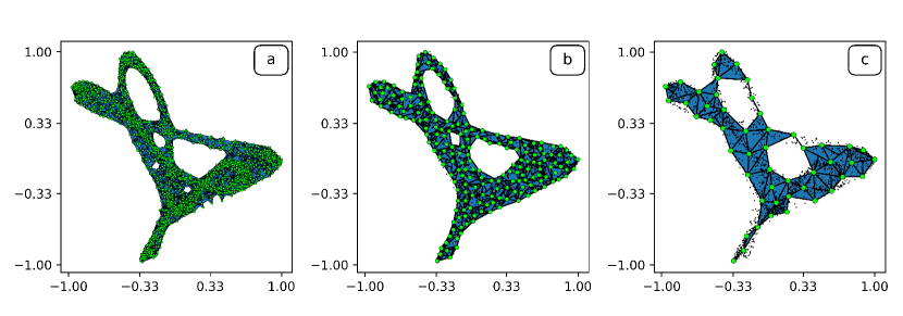
Figure 2: Different simplicial complexes built from the data set in Fig. 1(b) with $\epsilon=0.073$: (a) a Čech complex, with all $2000$ points used as vertices; (b) and (c) witness complexes with $\ell=200$ and $\ell=50$, respectively—i.e., with 1/10th and 1/40th of the points used as landmarks. Complexes (a) (b) and (c) contain $2770627$, $3938$, and $93$ triangles, respectively.

The distance checks involved in building such a complex—between all pairs of points, all triples, etc.—are computationally impractical for large data sets. There are many other ways to build simplicial complexes, including the $\alpha$-complex [8], the Vietoris-Rips complex [12], or even building a complex based on a cubical grid [13]. All of these approaches have major shortcomings for practical purposes: high computational cost, poor accuracy, and/or inapplicability in more than two dimensions.

An intriguing alternative is to coarse-grain the complex, employing a subset of the data points as vertices and using the rest to how to fill in the gaps. One way to do this is a witness complex [21], which is determined by the time-series data, $W$ (the witness set) and a smaller, associated set $L$—the landmarks, which form the vertices of the complex. Key elements of this process are the selection of appropriate landmarks, typically a subset of $W$, and a choice of a witness relation $R(W,L)\subset W\times L$, which determines how the simplices tile the landmarks: a point $w\in W$ is a witness to an abstract simplex $\sigma\in 2^{L}$ whenever $\{w\}\times\sigma\subset R(W,L)$. One connects two landmarks with an edge if they share at least one witness—this is a one-simplex. Similarly, if three landmarks have a common witness, they form a two-simplex, and so on. (This is similar to the Čech complex, except that not every point is a vertex.)

There are many ways to define what it means to share a witness. Informally, the rationale is that one wants to “fill in” the spaces between the vertices in the complex if there is at least one witness in the corresponding region. Following this reasoning, we could classify a witness $w_{i}\in W$ as shared by landmarks $l_{j},l_{k}\in L$ if $-\epsilon<|l_{j}-w_{i}|-|l_{k}-w_{i}|<\epsilon$—that is, if it is roughly equidistant to both of them—and add an edge to the complex if we find such a witness. If the set of witnesses included a point that were shared between three landmarks, we would add a face to the complex, and so on. That particular definition is problematic, however: it classifies an $\epsilon$-equidistant witness as shared even if it is on the opposite side of the data set from the two landmarks. To address this, we add a distance constraint to the witness relation, classifying a witness $w_{i}\in W$ as shared between two landmarks $l_{j},l_{k}\in L$ if both are within $\epsilon$ of being the closest landmark to $w_{i}$, i.e., if $\max(|l_{j}-w_{i}|,|l_{k}-w_{i}|)<\min_{m}|l_{m}-w_{i}|+\epsilon$:

Input: $\{x_{t}\}_{t=1}^{N}$, discrete $\mathbb{R}$-valued time series

delay coordinate reconstruction, $\{\textbf{x}_{t}\}_{t=d_{E}\tau}^{N}$

select landmarks $L=\{l_{i}\}_{i=1}^{\ell}\subseteq$ {x${}_{t}\}_{t=d_{E}\tau}^{N}$

compute pair-wise distances $D_{ij}=|l_{i}-\textbf{x}_{j}|$

for $\epsilon\in(\epsilon_{\text{min}},\epsilon_{\text{max}},\epsilon_{\text{step}}):$ (build witness complex, $\mathcal{W}^{\epsilon}$)

for $\textbf{x}_{t}\in X$:

$\text{d}=|L-\textbf{x}_{t}|+\epsilon$

for $(l_{i},l_{j})\in L:$    (check for edges)

if $|l_{i}-\textbf{x}_{t}|,|l_{j}-$x${}_{t}|<\text{d}:$

$\{l_{i},l_{j}\}\in\mathcal{W}^{\epsilon}$

for $(l_{i},l_{j},l_{k})\in L:$    (check for triangles)

if $|l_{i}-\textbf{x}_{t}|,|l_{j}-\textbf{x}_{t}|,|l_{k}-\textbf{x}_{t}|<\text{d}:$

$\{l_{i},l_{j},l_{k}\}\in\mathcal{W}^{\epsilon}$

⋮      (check for higher dimensional simplices)

Output: $\{\mathcal{W}^{\epsilon}\}_{\epsilon_{\text{min}}}^{\epsilon_{\text{max}}}$, series of witness complexes for specified $\epsilon$ range

Fig. 2(b) shows a witness complex constructed in this manner from the data of Fig. 2(a), with one-tenth of the points chosen as landmarks. The computation involved is much faster—an order of magnitude less than required for Fig. 2(a). The scale factor $\epsilon$ and the number $\ell$ of landmarks have critical implications for the correctness and complexity of this approach, as discussed further below.

Every simplicial complex has an associated set of homology groups, which depend upon the structure of the underlying manifold: whether or not it is connected, how many holes it has, etc. This is a potentially useful way to characterize and distinguish different regimes in data streams. An advantage of homology over homotopy or some other more complete topological theory is that it can be reduced to linear algebra [16]. Algorithms to compute homology depend on computing the null space and range of matrices that map simplices to their boundaries [13]. The computational complexity of these algorithms scales badly, though—both with the number of vertices in the complex and with the dimension of the underlying manifold. In view of this, the parsimonious nature of the witness complex is a major advantage. However, an overly parsimonious complex, or one that contains spurious simplices, may not capture the structure correctly.

The parsimony tradeoff plays out in the choices of both of the free parameters in this method. Fig. 2(b) and (c) demonstrate the effects of changing the number of vertices $\ell$ in the witness complex. With 200 vertices, the complex effectively captures the three largest holes in the delay reconstruction; if $\ell$ is lowered to 50, the complex is too coarse to capture the smallest of these holes. In general, increasing $\ell$ will improve the match of the complex to the data, but it will also increase the computational effort required to build and work with that structure. Reference [11] explores the accuracy end of this tradeoff; the computational complexity angle is covered in the later sections of this paper.

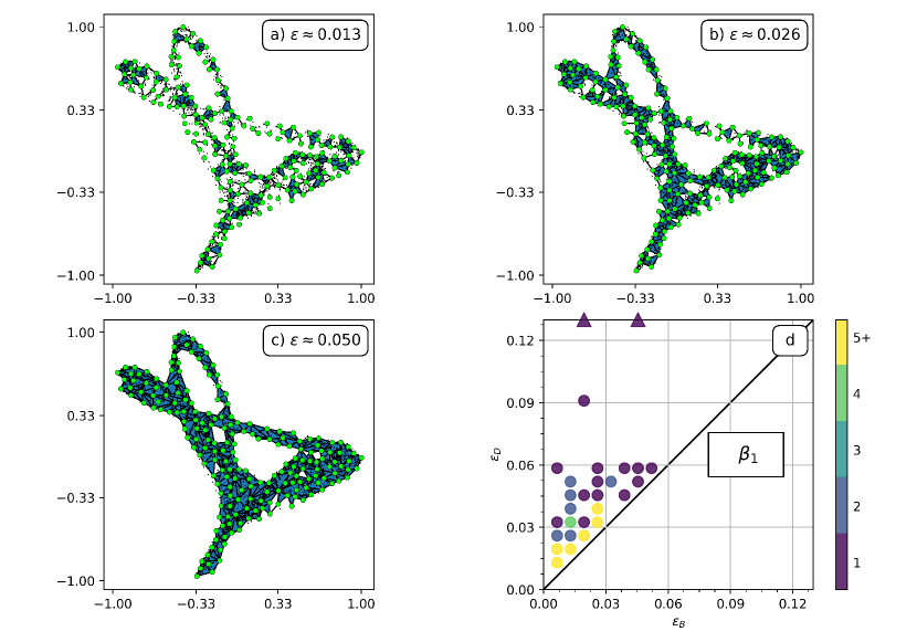
Figure 3: The effects of the scale parameter $\epsilon$: (a)-(c) show witness complexes with $\ell=200$ and different $\epsilon$ values. (d) shows a $\beta_{1}$ persistence diagram computed across a range of $\epsilon$ values. Each point in (d) represents a hole in the complex; its $x$ and $y$ coordinates show the $\epsilon$ values at which that hole appears and disappears, respectively. Holes that persist beyond the upper $\epsilon_{\text{max}}\approx 0.13$ are shown with triangles.

The other free parameter in the process, the scale factor $\epsilon$, plays a subtler and more interesting role. When $\epsilon$ is very small, as in Fig. 3(a), very few witnesses are shared and the complex is very sparse. As $\epsilon$ grows, more and more witnesses fall into the broadening regions that qualify them as shared, so more simplices appear in the complex, fleshing out the structure of the sampled manifold. There is a limit to this, however. When $\epsilon$ approaches the diameter of the point cloud, the witness complex will be fully connected, which obscures the native structure of the sampled set; well before that, simplices appear that do not reflect the true structure of the data. One effective way to track all of this is the $\beta_{1}$ persistence diagram of [7], which plots the $\epsilon$ value at which each hole appears in the complex, $\epsilon_{B}$, on the horizontal axis and the value $\epsilon_{D}$ at which it disappears from the complex on the vertical axis. A persistence diagram for the piano data, for example—part (d) of Fig. 3—shows a cluster of holes that are born and die before $\epsilon=0.06$. These represent small voids in the data. The three points near the top left of Fig. 3(d) represent holes that are highly persistent.

3 Persistent Homology and Membership Testing

Cycles are critical elements of the dynamical structure of many systems, and thus useful in distinguishing one system from another. A chaotic attractor, for example, is typically densely covered by unstable periodic orbits, and those orbits provide a formal “signature” of the corresponding system [3]. Topologically, a cycle is simply a hole, of any shape or size, in the state-space trajectory of the system. The persistent homology methods described above include some aspects of geometry, though, which makes the relationship between holes and cycles not completely simple. Musical instruments are an appealing testbed for exploring these issues. Of course, one can study the harmonic structure of a note from an instrument, or any other time series, using frequency analysis or wavelet transforms. Because delay reconstruction transforms time into space, it not only reveals which frequencies are present at which points in the signal, as well as their amplitudes. These reconstructions also bring out subtler features; any deviation from purely elliptical shape, for instance—or the kind of “winding” that appears on Fig. 1(b)—signals the presence of another signal and also gives some indication of its amplitude and relative frequency.

Topological data analysis brings out those kinds of features quite naturally. The structure of the persistence diagrams for the same note played on two different musical instruments, for instance, is radically different, as shown in Fig. 4. The witness complex of a clarinet playing the A above middle C contains seven holes for $\epsilon<0.05$. Six of these holes die before $\epsilon=0.06$; they are represented by the points in the lower left corner of the persistence diagram. The other hole in the complex triangulates the large loop in the center of the reconstruction of Fig. 4(a). This hole, which remains open until the end of the $\epsilon$ range of the calculation, is represented by the triangle in the top left corner of the persistence diagram in Fig. 4(c). The viol reconstruction in Fig. 4(b), on the other hand, contains over twelve holes that are born at low $\epsilon$ values, including many short-lived features depicted in the lower left of the persistence diagram. By $\epsilon=0.10$, only four holes remain open. The smallest of these four features, which closes up around $\epsilon=0.23$, is represented by the point in the top left of Fig. 4(d). The three other holes, which remain open to the end of the $\epsilon$ range of the calculation, are represented by the colored triangles at the top left of Fig. 4(d).

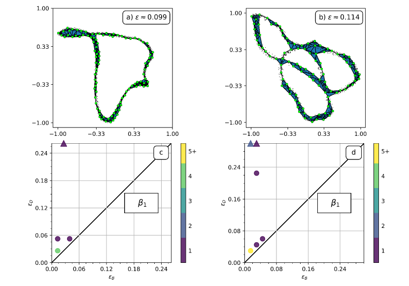
Figure 4: Witness complexes for A440 ($\mathfrak{f}=440$ Hz) played on a (a) clarinet and (b) viol constructed using $2000$ witnesses and $100$ landmarks for $\epsilon=0.099$, $0.114$ respectively. Beneath each are the corresponding $\beta_{1}$ persistence diagrams. The delay reconstructions are for approximately $0.05$ seconds each, with $\tau=\frac{1}{\mathfrak{f}\pi}$ seconds.

The patterns in these persistence diagrams—the number of highly persistent holes and short-lived features, and the $\epsilon$ values at which they appear and disappear—suggest that computational topology can be an effective way to distinguish between musical instruments. To test this more broadly, we built a pair of simple classifiers that work with persistent rank functions (PRFs), cumulative functions on $\mathbb{R}^{2+}$ that report the number and location of points in a persistence diagram [20]. We trained each classifier on 25 disjoint 0.05 sec windows from recordings of the corresponding instrument. This involved computing the persistent homology for each instance, then computing the mean, $\overline{\beta^{1}}$, and standard deviation, $\sigma$ of the set of corresponding PRFs. The test set comprised 50 0.05 sec windows, 25 from each instrument; for each of these samples, we computed the $L^{2}$ distance between the PRF of the sample and the mean $\overline{\beta^{1}}$ for each instrument. If that distance was below $k\sigma$ for some threshold parameter $k$, we assigned membership in the corresponding instrument class. The receiver operating characteristic (ROC) curves in the top row of Fig. 5 plot the true positive rates versus the false positive rates for the PRF classifiers. The clarinet classifier achieves a true positive rate 70% around $k=0.5$, and 100% when $k=1$. The false positive rate remains near 0% up through $k=5$, demonstrating a broad range of threshold values $k$ for which the PRF classifier will successfully assign membership in the clarinet class to most clarinet tones—and non-membership to most viol tones. The viol classifier achieves a true positive rate near 70% by $k=1$ and over 90% by $k=2$, maintaining a false positive rate below 50% for all $k$ up to $2.5$.

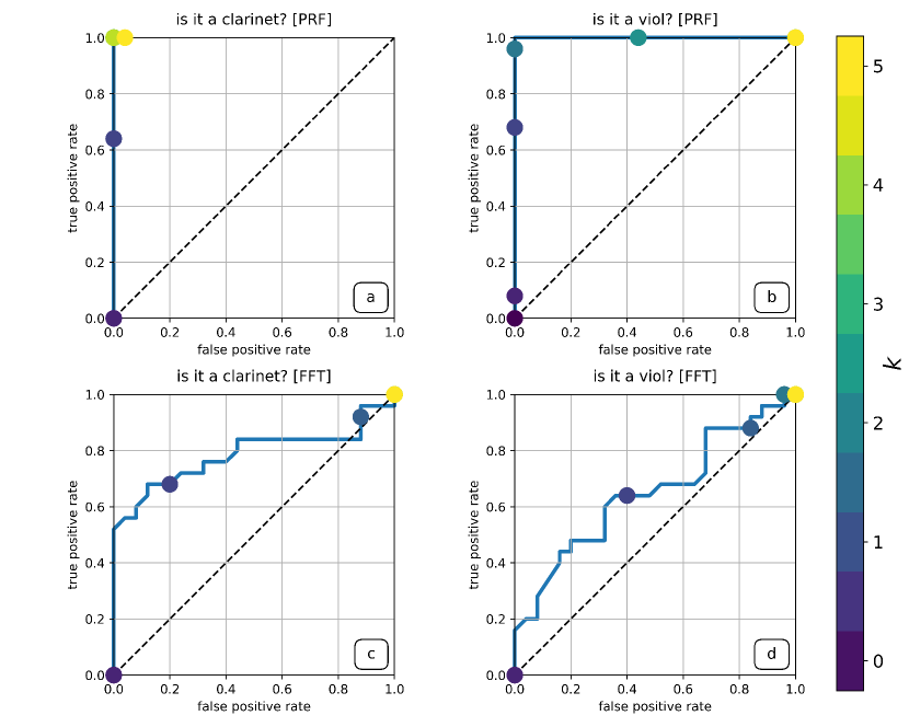
Figure 5: ROC curves for a persistent homology-based classifier (top) and an FFT-based classifier (bottom) for clarinet (left) and viol (right) membership testing. Color bar indicates the threshold parameter value $0<k<5$.

As a comparison, we built a pair of FFT-based classifiers, whose results are shown in the bottom row of Fig. 5, training and testing them on the same samples used for the PRF-based classifiers. The feature vector in this case was a set of 2000 logarithmically spaced values between 10 Hz and 10,000 Hz from the power spectrum of the signal. As in the PRF-based classifier, we computed the mean and standard deviation of this set of feature vectors, classifying a sample as a viol or clarinet if its $L^{2}$ distance to the corresponding mean feature vector was less than $k\sigma$. As is clear from the shapes of the ROC curves, the PRF-based classifiers outperformed the FFT-based classifiers. The FFT-based clarinet classifier achieves 70% and 20% true and false positive rates, respectively, around $k=0.5$. Above that threshold, the false positive rate rapidly catches up to the true positive rate, making the classifier equally likely to correctly classify a clarinet as a clarinet as it is to erroneously classify a viol as a clarinet. The ROC curve for the FFT-based viol membership classifier is even closer to the diagonal: it will correctly classify a viol as a viol only slightly more often than it will erroneously classify a clarinet as a viol, for any parameter value $0<k<5$.

Clarinets and viols produce very different sounds, of course, so distinguishing between them is not a hugely challenging task. A more interesting challenge is to compare two pianos. As shown in Fig. 6, persistence diagrams of the same note played on an upright piano and a grand piano are notably different: the former has a single long-lived hole—the fundamental tone of the note—while the latter has two, perhaps reflecting the greater sonic richness of the instrument. Persistence diagrams for both pianos contain many short-lived holes at low $\epsilon$ values, which also speaks to a notable variance in the volumes of the resonating frequencies.

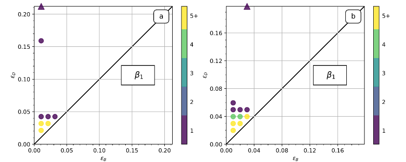
Figure 6: Persistence diagrams for A440 on two different pianos. (a): a Steinway grand piano; (b): a Baldwin upright piano.

Table 1 shows the runtime and memory costs involved in the construction of some of the complexes mentioned in this paper.

Number of landmarks	Runtime (sec)	Number of two-simplices	Memory usage
2000 (Čech)	59.1	2,770,627	9.3 MB
200	3.9	3,938	0.9 MB
50	0.8	93	$<$ 0.1 MB

Table 1: The computational and memory costs involved in constructing different simplicial complexes from the 2000-point reconstruction of Fig. 1(b) with $\epsilon=0.073$ on an Ubuntu Linux machine with an Intel Core i5 1.70GHz × 4 CPU and 12GB of memory.

These numbers make it quite clear why the parsimonious nature of the witness complex is so useful: using all of the points as landmarks is computationally prohibitive. And that parsimony, surprisingly, does not come at the expense of accuracy, as long as the samples satisfy some denseness constraints [1]. Nonetheless, this is still a lot of computational effort; the membership test process described here involves building the complex, computing the homology, repeating those calculations across a range of $\epsilon$ values, and perhaps computing a persistent rank function from the results. The associated runtime and memory costs will worsen with increasing $\epsilon$, and with the size of the data set, so computational topology is not the first choice technique for every IDA application. However, it can work when statistical- and frequency-based techniques do not.

4 Conclusion

We have shown that persistent homology can successfully distinguish musical instruments using witness complexes built from two-dimensional delay reconstructions for a single note. This approach does not rely on the linearity or data aggregation of many traditional membership-testing techniques; moreover, topological data analysis can outperform these traditional methods. Though the associated computations are not cheap, the reduction in model order and the parsimony of the witness complex greatly reduce the associated computational costs.

Persistent homology calculations—on any type of simplicial complex—work by blending geometry into topology via a scale parameter $\epsilon$. Their leverage derives from the patterns that one observes upon varying $\epsilon$, which are presented here in the form of persistence diagrams. The witness complex uses the scale parameter to obtain its natural parsimony. While the specific form of the witness relation used in this paper is a good start, it can still create holes where none “should” exist, and vice versa. Better witness relations—factoring in the temporal ordering and/or the forward images of the witnesses, or the curvature of those paths—will be needed to address those issues. This is particularly important in the context of the kinds of reduced-order models that we use here to further control the computational complexity. An incomplete delay reconstruction is a projection of a high-dimensional structure onto a lower-dimensional manifold: an action that can collapse holes, or create false ones. Changing $\tau$ also alters the geometry of a delay reconstruction. Understanding the interplay of geometry and topology in an incomplete embedding, and the way in which the witness relation exposes that structure, will be key to bringing topological data analysis into the practice of intelligent data analysis.

References

- [1] Alexander, Z., Bradley, E., Meiss, J., Sanderson, N.: Simplicial multivalued maps and the witness complex for dynamical analysis of time series. SIAM J. Appl. Dyn. Sys. 14, 1278–1307 (2015)
- [2] Bradley, E., Kantz, H.: Nonlinear time-series analysis revisited. Chaos 25(9), 097610 (2015)
- [3] Cvitanovic, P.: Invariant measurement of strange sets in terms of circles. Phys. Rev. Lett. 61, 2729–2732 (1988)
- [4] Dasu, T., Krishnan, S., Lin, D., Venkatasubramanian, S., Yi, K.: Change (detection) you can believe in: Finding distributional shifts in data streams. In: Advances in Intelligent Data Analysis, vol. 5572. Springer Lecture Notes in Computer Science (2009)
- [5] de Silva, V., Ghrist, R.: Coverage in sensor networks via persistent homology. Alg. Geom. Topology 7(1), 339–358 (2007)
- [6] Domingos, P.: A general framework for mining massive data streams. In: Proceedings Interface 2006 (2006)
- [7] Edelsbrunner, H., Letscher, D., Zomorodian, A.: Topological persistence and simplification. Disc. Comp. Geom. 28, 511–533 (2000)
- [8] Edelsbrunner, H., Mücke, E.: Three-dimensional alpha shapes. ACM Trans. Graphics 13, 43–72 (1994)
- [9] Fraser, A., Swinney, H.: Independent coordinates for strange attractors from mutual information. Phys. Rev. A 33(2), 1134–1140 (1986)
- [10] Gama, J.: Knowledge Discovery from Data Streams. Chapman and Hall/CRC (2010)
- [11] Garland, J., Bradley, E., Meiss, J.: Exploring the topology of dynamical reconstructions. Physica D 334, 49–59 (2014)
- [12] Ghrist, R.: Barcodes: The persistent topology of data. Bull. Amer. Math. Soc. 45(1), 61–75 (2008)
- [13] Kaczynski, T., Mischaikow, K., Mrozek, M.: Computational Homology, Appl. Math. Sci., vol. 157. Springer-Verlag, New York (2004)
- [14] Kennel, M.B., Brown, R., Abarbanel, H.D.I.: Determining minimum embedding dimension using a geometrical construction. Phys. Rev. A 45, 3403–3411 (1992)
- [15] Muldoon, M., MacKay, R., Huke, J., Broomhead, D.: Topology from a time series. Physica D 65, 1–16 (1993)
- [16] Munkres, J.: Elements of Algebraic Topology. Benjamin/Cummings, Menlo Park (1984)
- [17] Rakthanmanon, T., Keogh, E., Lonardi, S., Evans, S.: Time series epenthesis: Clustering time series streams requires ignoring some data. In: Proceedings ICDM, pp. 547–556. IEEE (Dec 2011)
- [18] Robins, V.: Computational topology for point data: Betti numbers of -shapes. In: Mecke, K., Stoyan, D. (eds.) Morphology of Condensed Matter, Lecture Notes in Physics, vol. 600, pp. 261–274. Springer Berlin Heidelberg (2002)
- [19] Robins, V., Abernethy, J., Rooney, N., Bradley, E.: Topology and intelligent data analysis. Intelligent Data Analysis 8, 505–515 (2004)
- [20] Robins, V., Turner, K.: Principal component analysis of persistent homology rank functions with case studies of spatial point patterns, sphere packing and colloids. Physica D 334, 99–117 (2015)
- [21] de Silva, V., Carlsson, E.: Topological estimation using witness complexes. In: Alexa, M., Rusinkiewicz, S. (eds.) Eurographics Symposium on Point-Based Graphics (2004), pp. 157–166. The Eurographics Association (2004)
- [22] Song, M., Wang, H.: Highly efficient incremental estimation of Gaussian mixture models for online data stream clustering. In: Priddy, K. (ed.) Proc. SPIE. vol. 5803, pp. 174–183. Intern. Soci. Optical Eng. (2005)
- [23] Xia, K., Feng, X., Tong, Y., Wei, G.: Persistent homology for the quantitative prediction of fullerene stability. J. Comput. Chem. 36(6), 408–422 (2015)
- [24] Zomorodian, A.: Topological Data Analysis, Advances in Applied and Computational Topology, vol. 70. Amer. Math. Soc. (2012)