On the quasi-Ablowitz-Segur and quasi-Hastings-McLeod solutions of the inhomogeneous Painlevé II equation

Abstract

We consider the quasi-Ablowitz-Segur and quasi-Hastings-McLeod solutions of the inhomogeneous Painlevé II equation

$$u^{\prime\prime}(x)=2u^{3}(x)+xu(x)-\alpha\qquad\textrm{for }\alpha\in\mathbb{R}\textrm{ and }|\alpha|>\frac{1}{2}.$$

These solutions are obtained from the classical Ablowitz-Segur and Hastings-McLeod solutions via the Bäcklund transformation, and satisfy the same asymptotic behaviors when $x\to\pm\infty$. For $|\alpha|>1/2$, we show that the quasi-Ablowitz-Segur and quasi-Hastings-McLeod solutions possess $[\,|\alpha|+\frac{1}{2}\,]$ simple poles on the real axis, which rigorously justifies the numerical results in Fornberg and Weideman (Found. Comput. Math., 14 (2014), no. 5, 985–1016).

2010 Mathematics Subject Classification. 33E17, 34M55.

Keywords and phrases: Painlevé II equation; Ablowitz-Segur solutions; Hastings-McLeod solutions; Bäcklund transformation.

 

$\ast$ Department of Mathematics, City University of Hong Kong, Hong Kong.
Email: dandai@cityu.edu.hk

${\dagger}$ Department of Mathematics, City University of Hong Kong, Hong Kong.
Email: weiyinghu2-c@my.cityu.edu.hk (corresponding author)

1 Introduction and statement of results

1.1 Ablowitz-Segur and Hastings-McLeod solutions

We consider the following inhomogeneous Painlevé II equation (PII)

$$u^{\prime\prime}(x)=2u^{3}+xu-\alpha,\qquad\alpha\in\mathbb{R}\setminus\{0\}.$$ (1.1)

When $\alpha=0$, the above equation is reduced to the homogeneous PII. It is well-known that, PII possesses two families of special solutions which are real and pole-free on the real axis: one family of these solutions is oscillatory and bounded, namely the Ablowitz-Segur (AS) solutions; the other family is smooth and nonoscillatory, namely the Hastings-McLeod (HM) solutions. Both families of solutions decay like $\alpha/x$ as $x\to+\infty$. More precisely, they have the following behaviors at $x\to\pm\infty$.

Ablowitz-Segur solutions: $\alpha\in(-1/2,1/2)$.

Let $k_{\alpha}$ be a real parameter and $k_{\alpha}\in(-\cos\pi\alpha,\cos\pi\alpha)$. The AS solution $u_{\textrm{AS}}(x;\alpha)$ is a one-parameter family of solutions of inhomogeneous PII (1.1), which is continuous on the real line and has the following asymptotic behaviors:

$$u_{\textrm{AS}}(x;\alpha) = B(x;\alpha)+k_{\alpha}\operatorname{{Ai}}(x)(1+O(x^{-3/4})),\qquad\textrm{as}\,\,x\to+\infty,$$ (1.2)

$$u_{\textrm{AS}}(x;\alpha) = \frac{d}{(-x)^{1/4}}\cos\{\frac{2}{3}(-x)^{3/2}-\frac{3}{4}d^{2}\ln(-x)+\phi\}+O(|x|^{-1}),$$

$$\hskip 184.9429pt\quad\textrm{as}\,\,x\to-\infty,$$

where $\operatorname{{Ai}}(x)$ is the Airy function,

$$B(x;\alpha)\sim\frac{\alpha}{x}\sum_{n=0}^{\infty}\frac{a_{n}}{x^{3n}},\qquad a_{0}=1$$ (1.4)

and $a_{n+1}=(3n+1)(3n+2)a_{n}-2\alpha^{2}\sum_{k,l,m=0}^{n}a_{k}a_{l}a_{m}.$ The constants $d$ and $\phi$ in (1.2) and (1.1) satisfy the following connection formulas

$$d(k_{\alpha}) = \frac{1}{\sqrt{\pi}}\sqrt{-\ln(\cos^{2}(\pi\alpha)-k_{\alpha}^{2})},$$ (1.5)

$$\phi(k_{\alpha}) = -\frac{3}{2}d^{2}\ln 2+\arg\Gamma{\biggr{(}\frac{1}{2}id^{2}}\biggr{)}-\frac{\pi}{4}-\arg(-\sin\pi\alpha-k_{\alpha}i).$$ (1.6)

Hastings-McLeod solutions: $\alpha\in\mathbb{R}$.

The HM solutions $u_{\textrm{HM}}(x;\alpha)$ of the inhomogeneous PII (1.1) are continuous on the real axis and have the following asymptotic behaviors

$$u_{\textrm{HM}}(x;\alpha) = B(x;\alpha)+\sigma\cos(\pi\alpha)\operatorname{{Ai}}(x)(1+O(x^{-3/4})),\qquad\textrm{as}\,\,x\to+\infty,$$ (1.7)

$$u_{\textrm{HM}}(x;\alpha) = \sigma\sqrt{\frac{-x}{2}}-\frac{\alpha}{2x}+O(-x)^{-3/2},\hskip 71.13188pt\qquad\textrm{as}\,\,x\to-\infty,$$ (1.8)

where $\sigma\in\{+1,-1\}$ and the series $B(x;\alpha)$ is given in (1.4). In (1.7) and (1.8), the coefficient $\sigma$ depends on $\alpha$ as follows:

$$\textrm{(i) if }\alpha>-1/2:\quad\sigma=+1;\qquad\textrm{(ii) if }\alpha<1/2:\quad\sigma=-1.$$ (1.9)

From the above formulas, one immediately sees that, when $\alpha\in(-\infty,-1/2]\cup[1/2,+\infty)$, there is a unique HM solution for each $\alpha$; while when $\alpha\in(-\frac{1}{2},\frac{1}{2})$, there exist two HM solutions. Depending on whether they are monotonic on the whole real axis, the solutions can be separated into two families, which are called the primary Hastings-McLeod solutions (pHM) and secondary Hastings-McLeod solutions (sHM) in Fornberg and Weideman [12]; see Figure 1 for a sketch of their properties. They satisfy the asymptotics in (1.7) and (1.8) with the parameter $\sigma$ given by

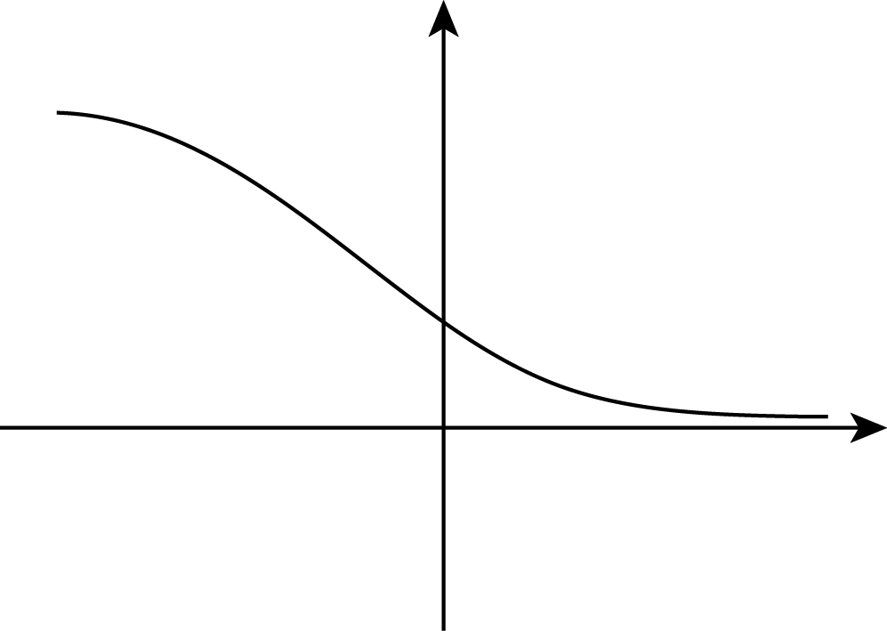
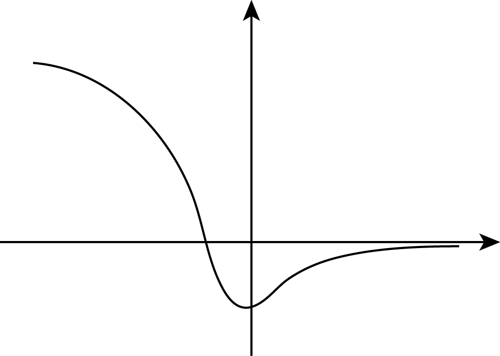
Figure 1: The pHM (left) $u_{\textrm{pHM}}(x;\alpha)$ and sHM (right) $-u_{\textrm{sHM}}(x;\alpha)$ solutions of PII with the same parameter $0<\alpha<1/2$.

pHM (monotonic): $$\sigma=\begin{cases}\textrm{sgn}(\alpha),&\textrm{if }\alpha\neq 0,\\ 1\textrm{ or }-1,&\textrm{if }\alpha=0,\end{cases}$$ (1.10)

sHM (not monotonic): $$\sigma=-\textrm{sgn}(\alpha),\qquad\textrm{if }\alpha\in(-1/2,0)\cup(0,1/2).$$ (1.11)

From (1.7)-(1.11), one can see that the pHM solutions have same signs in their asymptotic behaviors, i.e., $u_{\textrm{pHM}}(x;\alpha)\sim\alpha/x$ as $x\to+\infty$ and $u_{\textrm{pHM}}(x;\alpha)\sim\textrm{sgn}(\alpha)\sqrt{-x/2}$ as $x\to-\infty$ for $\alpha\neq 0$. This is similar to the classical HM solution $u_{\textrm{HM}}(x;0)$ of the homogeneous PII whose asymptotic behaviors are $u_{\textrm{HM}}(x;0)\sim\operatorname{{Ai}}(x)$ as $x\to+\infty$ and $u_{\textrm{HM}}(x;\alpha)\sim\sqrt{-x/2}$ as $x\to-\infty$. It is well-known that the HM solution $u_{\textrm{HM}}(x;0)$ is monotonic on the real axis and possesses a unique inflexion point $x_{0}$ where $u_{\textrm{HM}}^{\prime\prime}(x_{0};0)=0$; see Hastings and McLeod [15]. From the numerical evidence in Fornberg and Weideman [12, Fig. 10], the pHM solutions satisfy similar properties. For the sHM solutions, they have different signs in their asymptotics as $x\to\pm\infty$, and are no longer monotonic. Recently, these properties have been proved rigorously in Clerc et al. [6] and Troy [21].

The formulas (1.10) and (1.11) indicate that there exists a family of pHM solutions for any $\alpha\in\mathbb{R}$; and there is one additional family of sHM solutions for $\alpha\in(-1/2,0)\cup(0,1/2)$. This result is actually proved in Claeys, Kuijlaars and Vanlessen [3, Theorem 1.1]. In [3], the authors showed that, for $\alpha>-1/2$, there exist the HM solutions which are pole-free on the real line and uniquely determined by the following asymptotic behaviors

$$u(x;\alpha)\sim\alpha/x,\quad\textrm{as }x\to+\infty\quad\textrm{and}\quad u(x;\alpha)\sim\sqrt{-x/2},\quad\textrm{as }x\to-\infty.$$

With the classification in (1.10) and (1.11), one can see that the above solutions are indeed the pHM and sHM solutions when $\alpha>0$ and $-1/2<\alpha<0$, respectively. Using the following symmetry relation

$$u(x;\alpha)=-u(x;-\alpha),$$ (1.12)

one immediately gets the pHM and sHM solutions for $\alpha<0$ and $0<\alpha<1/2$.

The AS and HM solutions for the homogeneous PII were first discovered by Ablowitz and Segur in [1, 20] and Hastings and McLeod in [15], respectively. For the inhomogeneous PII, these solutions were obtained later by McCoy and Tang [19], Its and Kapaev [16] and Kapaev [18]. The rigorous justification of the asymptotic behaviors in (1.2)-(1.1) and (1.7)-(1.8), as well as the connection formulas (1.5)-(1.6), has attracted a lot of research interest in the literature; see for example [2, 5, 8, 17] and the monograph by Fokas et al. [10]. All the AS and HM solutions are pole-free on the real axis; see Claeys, Kuijlaars and Vanlessen [3] and Dai and Hu [7]. It is very interesting to note that these pHM and sHM solutions for the inhomogeneous PII play an important role in the study of nematic liquid crystals; see [6, 21]. Recently, some novel solutions similar to the AS and HM solutions are obtained by Fornberg and Weideman [12]. They are no longer pole-free but have finitely many poles on the real axis. We will discuss them in the coming section.

1.2 Quasi-Ablowitz-Segur and quasi-Hastings-McLeod solutions

It is a well-known fact that, PII transcendents for different parameters $\alpha$ are related to each other through the following Bäcklund transformation:

$$u(x;\alpha)=-u(x;\alpha-1)+\frac{2\alpha-1}{2u^{2}(x;\alpha-1)-2u^{\prime}(x;\alpha-1)+x};$$ (1.13)

see [4]. From the previous section, we know that the AS and sHM solutions exist only when $|\alpha|<1/2$. Applying the Bäcklund transformation to the AS and sHM solutions, we will get solutions for $|\alpha|>1/2$. It is very interesting to see that the asymptotic behaviors as $x\to\pm\infty$ are reserved under the Bäcklund transformation (1.13). The only difference is that, due to properties of the denominator

$$f(x;\alpha):=2u^{2}(x;\alpha)-2u^{\prime}(x;\alpha)+x,$$ (1.14)

the solutions after the Bäcklund transformation may not be pole-free on the real line. Fornberg and Weideman first observe such kind of solutions and name them the quasi-Ablowitz-Segur (qAS) and quasi-Hastings-McLeod (qHM) solutions; see [12, Sec. 4.3].

Let us define the qAS and qHM solutions with more details below. Due to the symmetry relation (1.12), we may assume $\alpha>0$.

qAS solutions: $\alpha\in(n-1/2,n+1/2),$ $n\in\mathbb{N}$.

Let $k_{\alpha}$ be a real parameter and $k_{\alpha}\in(-|\cos\pi\alpha|,|\cos\pi\alpha|)$. The qAS solution $u_{\textrm{qAS}}(x;\alpha)$ is a one-parameter family of solutions of inhomogeneous PII (1.1), which satisfies the asymptotic behaviors in (1.2) and (1.1), as well as the connection formulas (1.5) and (1.6).

qHM solutions: $\alpha\in(n-1/2,n+1/2),$ $n\in\mathbb{N}$.

The qHM solutions $u_{\textrm{qHM}}(x;\alpha)$ of the inhomogeneous PII (1.1) have the following asymptotic behaviors

$$u_{\textrm{qHM}}(x;\alpha) = B(x;\alpha)-\cos(\pi\alpha)\operatorname{{Ai}}(x)(1+O(x^{-3/4})),\qquad\textrm{as}\,\,x\to+\infty,$$ (1.15)

$$u_{\textrm{qHM}}(x;\alpha) = -\sqrt{\frac{-x}{2}}-\frac{\alpha}{2x}+O(-x)^{-3/2},\hskip 71.13188pt\quad\textrm{as}\,\,x\to-\infty,$$ (1.16)

where the series $B(x;\alpha)$ is given in (1.4).

Remark 1.

The qHM solutions distinguish themselves from the pHM solutions in (1.10) for $\alpha>1/2$ by having different signs in their asymptotics as $x\to\pm\infty$.

Remark 2.

If one applies the Bäcklund transformation to the HM solutions $u_{\textrm{HM}}(x;\alpha)$ (including all the pHM, sHM and qHM solutions) to get a solution $u(x;\alpha+1)$, it is straightforward to verify that the leading term of the asymptotics at $-\infty$ is still $\textrm{sgn}(\alpha)\sqrt{-x/2}$ for $\alpha\neq 0$; while the leading term of the asymptotics at $+\infty$ becomes $(\alpha+1)/x$. Therefore, because the asymptotics of $u(x;\alpha+1)$ as $x\to\pm\infty$ keep the same sign for $\alpha>0$, we have

$$\begin{array}[]{l}u_{\textrm{pHM}}(x;\alpha)\mapsto u_{\textrm{pHM}}(x;\alpha+1),\\ u_{\textrm{sHM}}(x;\alpha)\textrm{ and }u_{\textrm{qHM}}(x;\alpha)\mapsto u_{\textrm{qHM}}(x;\alpha+1),\end{array}\qquad\textrm{for }\alpha>0.$$ (1.17)

Since the term $\alpha/x\mapsto(\alpha+1)/x$ changes sign when $-1/2<\alpha<0$, we obtain

$$u_{\textrm{pHM}}(x;\alpha)\mapsto u_{\textrm{qHM}}(x;\alpha+1),\quad u_{\textrm{sHM}}(x;\alpha)\mapsto u_{\textrm{pHM}}(x;\alpha+1)\quad\textrm{for }-1/2<\alpha<0.$$ (1.18)

For the case $\alpha=0$, if we choose the following pHM solution with $\sigma=-1$ in (1.10)

$$u_{\textrm{pHM}}(x;0)\sim-\operatorname{{Ai}}(x),\quad\textrm{as }x\to+\infty\quad\textrm{and}\quad u_{\textrm{pHM}}(x;0)\sim-\sqrt{-x/2},\quad\textrm{as }x\to-\infty,$$ (1.19)

then the Bäcklund transformation (1.13) gives us

$$u(x;1)\sim 1/x,\quad\textrm{as }x\to+\infty\quad\textrm{and}\quad u(x;1)\sim-\sqrt{-x/2},\quad\textrm{as }x\to-\infty,$$ (1.20)

which is $u_{\textrm{qHM}}(x;1)$. Of course, if we put $\sigma=1$, we get $u_{\textrm{pHM}}(x;1)$.

Remark 3.

When applying the Bäcklund transformation to get the qAS solutions, we have

$$\alpha\mapsto\alpha+1\qquad\textrm{and}\qquad k_{\alpha}\mapsto k_{\alpha+1}\ \textrm{ with }k_{\alpha+1}=-k_{\alpha},$$ (1.21)

where $k_{\alpha}$ is given in (1.2). Similar sign change for the coefficient of the $\operatorname{{Ai}}(x)$ term also occurs while obtaining the qHM solutions, where $\cos(\pi\alpha)$ is mapped to $\cos(\pi(\alpha+1))$ in (1.7) and (1.15).

It is interesting to note that any qAS and qHM solutions defined above admit a Bäcklund transformation (1.13) with the Ablowitz-Segur or Hastings-McLeod solution as the seed solution. To see this, one can study the Bäcklund transformation (1.13) through Riemann-Hilbert (RH) problems; see Fokas et al. [10, Sec. 6.1]. The AS(qAS) solutions correspond to the following special Stokes multipliers

$$s_{1}=-\sin(\pi\alpha)-ik_{\alpha},\quad s_{2}=0,\quad s_{3}=-\sin(\pi\alpha)+ik_{\alpha},\quad k_{\alpha}\in(-|\cos\pi\alpha|,|\cos\pi\alpha|)$$ (1.22)

see [7, (2.20)]. When we change the parameters as in (1.21), the Stokes multipliers become $s_{k}\mapsto-s_{k}$, $k=1,3$. Studying the difference between the two associated RH problems, we get the Bäcklund transformation (1.13). Moreover, once the Stokes multipliers are fixed for the qAS solutions $u_{\textrm{qAS}}(x;\alpha)$, the asymptotics in (1.2) and (1.1) can be derived by using Deift-Zhou nonlinear steepest method uniquely; see for example [7, 8, 16, 18]. Similar arguments also work for the qHM solutions $u_{\textrm{qHM}}(x;\alpha)$. Since we focus on the pole properties of the qAS and qHM solutions, we will not go into the detailed RH analysis in this paper.

1.3 Our main results

We will prove the following results about the poles of qAS and qHM solutions.

Theorem 1.

For $\alpha\in(n-\frac{1}{2},n+\frac{1}{2})$ with $n\in\mathbb{N}$, let the qAS solutions $u_{\textrm{qAS}}(x;\alpha)$ and qHM solutions $u_{\textrm{qHM}}(x;\alpha)$ be the solution of PII (1.1) with asymptotic behaviors given in (1.2)-(1.1) and (1.15)-(1.16), respectively. Then, the qAS and qHM solutions have $n$ real poles.

Remark 4.

Pole numbers of the qAS and qHM solutions on the real line have been predicted by Fornberg and Weideman based on the numerical computations in [12]. In the past a few years, Fornberg and Weideman [11, 13] have successfully developed the pole field solver (PFS) to compute the Painlevé transcendents in the complex plane efficiently and accurately. Recently, they further extend the PFS to study multivalued Painlevé transcendents on their Riemann surfaces; see Fasondini, Fornberg and Weideman [9] .

Besides the pole numbers, our analysis gives more properties about the poles on the real axis. It is well-known that the PII transcendents are meromorphic functions whose poles are all simple with residue $\pm 1$; see Gromak et al. [14, Sec. 2]. Our second result shows the dynamics of these poles with respect to the parameter $\alpha$.

Theorem 2.

For $\alpha\in(n-\frac{1}{2},n+\frac{1}{2})$ with $n\in\mathbb{N}$, let $p_{i,\pm 1}(\alpha)$ be the $i$-th real pole of $u_{\textrm{qAS}}(x;\alpha)$ or $u_{\textrm{qHM}}(x;\alpha)$ counting from the negative real axis, where the subscript $\pm 1$ indicates the residue of the pole is 1 or $-1$. Then, the poles $p_{i,\pm 1}(\alpha)$ satisfy the following properties:

• The residue of the smallest pole must be 1. Moreover, it is strictly decreasing with respect to $\alpha$, i.e.,

  $$p_{1,+1}(\alpha)>p_{1,+1}(\alpha+1)>p_{1,+1}(\alpha+2)>\cdots.$$ (1.23)

• The poles with residue $\pm 1$ interlace on the real axis, that is,

  $$\begin{split}&p_{1,+1}(\alpha)<p_{2,-1}(\alpha)<\cdots<p_{n,+1}(\alpha),\quad\textrm{if $n$ is odd,}\\ &p_{1,+1}(\alpha)<p_{2,-1}(\alpha)<\cdots<p_{n,-1}(\alpha),\quad\textrm{if $n$ is even.}\end{split}$$ (1.24)

• All poles of $u(x;\alpha)$ with residue $+1$ become poles of $u(x;\alpha+1)$ with residue $-1$ via the Bäcklund transformation, i.e. $p_{i+1,-1}(\alpha+1)=p_{i,+1}(\alpha)$; while all poles of $u(x;\alpha)$ with residue $-1$ are regular points of $u(x;\alpha+1)$.

• The residue of the largest pole is $1$ and $-1$ when $n$ is odd and even, respectively. They are increasing with respect to $\alpha$

  $$\begin{split}&p_{n,+1}(\alpha)=p_{n+1,-1}(\alpha+1)<p_{n+2,+1}(\alpha+2)=p_{n+3,-1}(\alpha+3)<\cdots,\quad\textrm{if $n$ is odd},\\ &p_{n,-1}(\alpha)<p_{n+1,+1}(\alpha+1)=p_{n+1,-1}(\alpha+2)<\cdots,\hskip 88.2037pt\quad\textrm{if $n$ is even}.\end{split}$$ (1.25)

The properties in the above theorems can be summarized in the following figure.

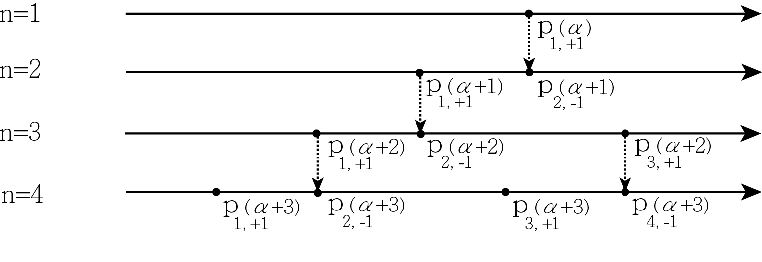
Figure 2: The poles locations of qAS and qHM solutions of PII on $\mathbb{R}$.

The rest of this paper is arranged as follows. In Section 2, some properties for the general PII transcendent $u(x;\alpha)$ and the function $f(x;\alpha)$ in (1.14) are provided. Then, in Section 3, we prove our main results by mathematical induction.

2 Properties of the general PII transcendents

First, let us derive some relations between a general solution $u(x;\alpha)$ and the denominator $f(x;\alpha)$ in the Bäcklund transformation (1.13).

Lemma 1.

The functions $u(x;\alpha)$ and $f(x;\alpha)$ satisfy the following relations:

• If $u(x;\alpha)$ is continuous and differentiable at $x_{0}$ such that $f(x_{0};\alpha)=0$, then $f^{\prime}(x_{0};\alpha)=2\alpha+1$.

• In any interval where $u(x;\alpha)$ is continuous, $f(x;\alpha)$ has at most one simple zero when $\alpha\neq-1/2$.

Proof.

From the definition of $f(x;\alpha)$ in (1.14), we have

$$f^{\prime}(x;\alpha)=4u^{\prime}(x;\alpha)u(x;\alpha)-2u^{\prime\prime}(x;\alpha)+1.$$

As $u(x;\alpha)$ satisfies the PII equation (1.1), it follows from the above formula

$$f^{\prime}(x;\alpha)=-2u(x;\alpha)f(x;\alpha)+2\alpha+1.$$ (2.1)

This immediately gives us part (i) of the lemma.

We will prove the second part by contradiction. Suppose that there are two adjacent zeros $x_{0}$ and $\tilde{x}_{0}$ of $f(x;\alpha)$ in the interval $I$ where $u(x;\alpha)$ is continuous. According to the definition of $f(x;\alpha)$ in (1.14), we know $f(x;\alpha)$ is continuous and differentiable in $I$. If $\alpha\neq-1/2$, then the zeros of $f(x;\alpha-1)$ must be simple, since

$$f^{\prime}(x;\alpha)=2\alpha+1\neq 0.$$ (2.2)

Thus, we have

$$f(x_{0};\alpha)=f(\tilde{x}_{0};\alpha)=0\quad\textrm{and}\quad f^{\prime}(x_{0};\alpha)f^{\prime}(\tilde{x}_{0};\alpha)<0.$$

However, part (i) of the lemma also tells us

$$f^{\prime}(x_{0};\alpha)=f^{\prime}(\tilde{x}_{0};\alpha)=2\alpha+1,$$ (2.3)

which yields a contradiction. Therefore, $f(x;\alpha)$ has at most one zero in $I$. ∎

Next, we study the pole properties under the Bäcklund transformation.

Lemma 2.

Let the solutions $u(x;\alpha-1)$ and $u(x;\alpha)$ be related via the Bäcklund transformation (1.13). Then, we have

• The poles of $u(x;\alpha-1)$ with residue $+1$ are poles of $u(x;\alpha)$ with residue $-1$.

• If $p_{-1}$ is a pole of $u(x;\alpha-1)$ with residue $-1$, then $p_{-1}$ is a regular point of $u(x;\alpha)$.

Proof.

To prove part (i), let us assume $p_{+1}$ is a pole of $u(x;\alpha-1)$ with residue $+1$. Then we have the following expansion near $p_{+1}$

$$u(x;\alpha-1)=\frac{1}{x-p_{+1}}-\frac{p_{+1}}{6}(x-p_{+1})+\frac{\alpha-2}{4}(x-p_{+1})^{2}+O((x-p_{+1})^{3}),\qquad\textrm{as }x\to p_{+1}.$$ (2.4)

Using the definition of $f(x;\alpha)$ in (1.14) and the above formula, we can see that $p_{+1}$ is a double pole of $f(x;\alpha-1)$:

$$f(x;\alpha-1)=\frac{4}{(x-p_{+1})^{2}}+O((x-p_{+1})^{-3}),\qquad\textrm{as }x\to p_{+1}.$$ (2.5)

From the Bäcklund transformation (1.13), it is easy to obtain

$$u(x;\alpha)=-\frac{1}{x-p_{+1}}+\frac{p_{+1}}{6}(x-p_{+1})+\frac{\alpha+1}{4}(x-p_{+1})^{2}+O((x-p_{+1})^{3}),\qquad\textrm{as }x\to p_{+1}.$$ (2.6)

Therefore, $p_{+1}$ is a pole of $u(x;\alpha)$ with residue $-1$.

Similarly, we can prove part (ii). If $p_{-1}$ is a pole of $u(x;\alpha-1)$ with residue $-1$, the following expansion near $p_{-1}$ holds:

$$u(x;\alpha-1)=\frac{-1}{x-p_{-1}}+\frac{p_{-1}}{6}(x-p_{-1})+\frac{\alpha}{4}(x-p_{-1})^{2}+O((x-p_{-1})^{3}),\qquad\textrm{as }x\to p_{-1}.$$ (2.7)

Then, $p_{-1}$ is a simple zero of $f(x;\alpha-1)$:

$$f(x;\alpha-1)=(-2\alpha+1)(x-p_{-1})+O((x-p_{-1})^{2}),\qquad\textrm{as }x\to p_{-1}.$$ (2.8)

As a consequence, the second term in the Bäcklund transformation (1.13) induces a simple pole with residue $-1$, which cancels the pole contribution from the first term. Thus, $p_{-1}$ is a regular point of $u(x;\alpha)$. ∎

3 Proof of Theorems 1 and 2

3.1 Properties of real poles of qAS solutions

For $\alpha\in(n-\frac{1}{2},n+\frac{1}{2})$, we will study the qAS solutions for $n=1,2,3$, which possess all properties listed in Theorems 1 and 2. Then, we will prove our results by mathematical induction for all $n\in\mathbb{N}$. First, we show that, for $\alpha\in(\frac{1}{2},\frac{3}{2})$, the qAS solutions have only one pole on the real line.

Proposition 1.

For $\alpha\in(\frac{1}{2},\frac{3}{2})$, the qAS solutions of (1.1) have only one pole on the real line with residue $+1$.

Proof.

For $\alpha\in(\frac{1}{2},\frac{3}{2})$, $u_{\textrm{AS}}(x;\alpha-1)$ is the pole-free AS solution on the real line. To get the unique pole of $u_{\textrm{qAS}}(x;\alpha)$, it is enough to show that $f(x;\alpha-1)$ in the Bäcklund transformation (1.13) has only one zero on the real line. Recalling the asymptotics of $u_{\textrm{AS}}(x;\alpha-1)$ in (1.2) and (1.1), we have from (1.14)

$$f(x;\alpha-1)\sim x,\qquad\textrm{as}\,\,x\to\pm\infty.$$ (3.1)

Moreover, since $u_{\textrm{AS}}(x;\alpha-1)$ is smooth on the real line, $f(x;\alpha-1)$ is also continuous on the real line. The above asymptotics imply that $f(x;\alpha-1)$ has zeros on the real line.

According Lemma 1, there is a unique point $x_{1}$ such that $f(x_{1};\alpha-1)=0$ and $f^{\prime}(x_{1},\alpha-1)=2\alpha-1$. Then, using the Bäcklund transformation (1.13), we conclude that $u_{\textrm{qAS}}(x;\alpha)$ has only one pole on the real line with residue $+1$. ∎

Proposition 2.

For $\alpha\in(\frac{3}{2},\frac{5}{2})$, the qAS solutions of (1.1) have two poles on the real line with residues $\pm 1$. Moreover, we have $p_{1,+1}(\alpha)<p_{2,-1}(\alpha)$.

Proof.

For $\alpha\in(\frac{3}{2},\frac{5}{2})$, let $x_{1,+1}$ be the unique pole of $u_{\textrm{qAS}}(x;\alpha-1)$ with residue $+1$. Then, from part (i) in Lemma 2, $x_{1,+1}$ is the pole of $u_{\textrm{qAS}}(x;\alpha)$ with residue $-1$. To find the other pole of $u_{\textrm{qAS}}(x;\alpha)$, we make use of the behavior of $u_{\textrm{qAS}}(x;\alpha-1)$ near $x_{1,+1}$ given in (2.4). Combining the formulas (1.2)-(1.1), we have from (1.14)

$$f(x;\alpha-1)\sim x,\qquad\textrm{as}\,\,x\to\pm\infty\quad\textrm{and}\quad f(x;\alpha-1)\to+\infty,\qquad\textrm{as}\,\,x\to x_{1,+1}.$$ (3.2)

Based on the similar analysis in Proposition 1, we get that $f(x;\alpha-1)$ has only one zero $x_{0}$ in $(-\infty,x_{1,+1})$ and $f^{\prime}(x_{0};\alpha-1)=2\alpha-1$. Therefore, $x_{0}$ is the unique pole of $u_{\textrm{qAS}}(x;\alpha)$ in $(-\infty,x_{1,+1})$ with residue $+1$.

Finally, to show that there is no other poles, we verify that $u_{\textrm{qAS}}(x;\alpha)$ has no pole in $(x_{1,+1},+\infty)$. Otherwise, $f(x;\alpha-1)$ must have zeros in $(x_{1,+1},+\infty)$. Due to the asymptotics in (3.2), $f(x;\alpha-1)$ tends to $+\infty$ at both endpoints of the interval $(x_{1,+1},+\infty)$. Then, $f(x;\alpha-1)$ has at least two zeros in $(x_{1,+1},+\infty)$, where we use the fact that all zeros of $f(x;\alpha-1)$ are simple. So, we arrive at a contradiction with part (ii) of Lemma 1.

This completes the proof of our proposition. ∎

Proposition 3.

For $\alpha\in(\frac{5}{2},\frac{7}{2})$, the qAS solutions of (1.1) have three poles on the real line with residues $\pm 1$. Moreover, we have $p_{1,+1}(\alpha)<p_{2,-1}(\alpha)<p_{3,+1}(\alpha)$.

Proof.

For $\alpha\in(\frac{5}{2},\frac{7}{2})$, let $x_{1,+1}<x_{2,-1}$ be the two poles of $u_{\textrm{qAS}}(x;\alpha-1)$ with residues $+1$ and $-1$, respectively. Then, from part (i) in Lemma 2, $x_{1,+1}$ is the pole of $u_{\textrm{qAS}}(x;\alpha)$ with residue $-1$. Using the similar analysis in Proposition 2, it is easy to show that there is a unique pole of $u_{\textrm{qAS}}(x;\alpha)$ in $(-\infty,x_{1,+1})$ with residue $+1$. To find the last pole of $u_{\textrm{qAS}}(x;\alpha)$, let us study the property of $f(x;\alpha-1)$ in $(x_{1,+1},+\infty)$. Using a similar computation in (3.2), we have

$$f(x;\alpha-1)\to+\infty,\quad\textrm{as }x\to x_{1,+1},\quad\textrm{and}\quad f(x;\alpha-1)\to+\infty,\quad\textrm{as }x\to+\infty.$$ (3.3)

Note that, although $x_{2,-1}\in(x_{1,+1},+\infty)$, it is a regular point of $u_{\textrm{qAS}}(x;\alpha)$; see part (ii) of Lemma 2. Moreover, we have from (2.8)

$$f(x_{2,-1};\alpha-1)=0\quad\textrm{and}\quad f^{\prime}(x_{2,-1};\alpha-1)=-2\alpha+1<0.$$ (3.4)

As $f(x;\alpha-1)$ is continuous and differentiable on $(x_{1,+1},+\infty)$, the above two formulas yield there must exist $x_{3}>x_{2,-1}$ such that $f(x_{3};\alpha-1)=0$ and $f^{\prime}(x_{3};\alpha-1)>0$. Note that $u_{\textrm{qAS}}(x;\alpha-1)$ is continuous on $(x_{2,-1},+\infty)$. According to Lemma 1, $x_{3}$ is the unique zero of $f(x;\alpha-1)$ in $(x_{2,-1},+\infty)$ and $f^{\prime}(x_{3};\alpha-1)=2\alpha-1$. Therefore, $x_{3}$ must be a pole of $u_{\textrm{qAS}}(x;\alpha)$ with residue $+1$. By Lemma 1 again, $u_{\textrm{qAS}}(x;\alpha)$ has no pole in $(x_{1,+1},x_{2,-1})$.

This completes the proof of our proposition. ∎

Finally, we prove the statements involving the qAS solutions in Theorems 1 and 2 by mathematical induction.

Proof of Theorem 1 and 2. The above three propositions indicate that Theorems 1 and 2 are true for $n=1,2,3$. Assume the results also hold for $n=m$, let us consider the case for $m+1$. We denote the poles of $u_{\textrm{qAS}}(x;\alpha)$ and $u_{\textrm{qAS}}(x;\alpha+1)$ by $p_{i,\pm 1}(\alpha)$ and $\widetilde{p}_{j,\pm 1}(\alpha+1)$, respectively.

As the residue of the smallest pole of $u_{\textrm{qAS}}(x;\alpha)$ is 1, following similar analysis in Proposition 2, there exists a unique pole $x_{0}$ of $u_{\textrm{qAS}}(x;\alpha+1)$ in $(-\infty,p_{1,+1}(\alpha))$ with residue $1$. This proves part (a) of Theorem 2.

Let $p_{k,+1}(\alpha)<p_{k+1,-1}(\alpha)<p_{k+2,+1}(\alpha)$ be three consecutive poles of $u_{\textrm{qAS}}(x;\alpha)$. According to Lemma 2, they are mapped to $\widetilde{p}_{j,-1}(\alpha+1)<\eta_{0}<\widetilde{p}_{j+2,-1}(\alpha+1)$, where $\eta_{0}$ is the zero of $f(x;\alpha)$ and a regular point of $u_{\textrm{qAS}}(x;\alpha+1)$. Since $p_{k,+1}(\alpha)$ and $p_{k+2,+1}(\alpha)$ are poles of $u_{\textrm{qAS}}(x;\alpha)$ with residue $+1$, we have from (2.5)

$$f(x;\alpha)\to+\infty,\quad\textrm{as }x\to p_{k,+1}(\alpha)\textrm{ and }x\to p_{k+2,+1}(\alpha).$$ (3.5)

Using the similar analysis in Proposition 3, there exists a unique point $x^{*}\in(p_{k+1,-1}(\alpha),p_{k+2,+1}(\alpha))$ such that $f(x^{*};\alpha)=0$ and $f^{\prime}(x^{*};\alpha)=2\alpha+1>0$. This shows that $x^{*}$ is the unique pole of $u_{\textrm{qAS}}(x;\alpha+1)$ with residue $+1$ in $(\eta_{0},\widetilde{p}_{j+2,-1}(\alpha+1))$. Therefore, we obtain three consecutive poles of $u_{\textrm{qAS}}(x;\alpha+1)$: $\widetilde{p}_{j,-1}(\alpha+1)<\widetilde{p}_{j+1,+1}(\alpha+1)<\widetilde{p}_{j+2,-1}(\alpha+1)$ with $\widetilde{p}_{j+1,+1}(\alpha+1)=x^{*}$. Thus, we prove the interlacing property of poles with residue $\pm 1$, i.e., part (b) of Theorem 2. The part (c) of Theorem 2 is indeed Lemma 2.

The proof of the pole numbers and the largest pole also follows from the arguments above. Lemma 2 and arguments in the previous paragraph imply that, for the interval $I=[p_{k_{1},+1}(\alpha),p_{k_{2},+1}(\alpha)]$ with any $k_{1}<k_{2}$, $u_{\textrm{qAS}}(x;\alpha+1)$ has the same number of poles as $u_{\textrm{qAS}}(x;\alpha)$ in $I$. When $m$ is odd, as the residues of both the smallest and largest pole of $u_{\textrm{qAS}}(x;\alpha)$ are 1, $u_{\textrm{qAS}}(x;\alpha+1)$ has $m$ poles in $[p_{1,+1}(\alpha),p_{m,+1}(\alpha)]$ with ${p}_{2,-1}(\alpha+1)=p_{1,+1}(\alpha)$ and ${p}_{m+1,-1}(\alpha+1)=p_{m,+1}(\alpha)$. Recalling that there is one more pole with residue 1 in $(-\infty,p_{1,+1}(\alpha))$, then $u_{\textrm{qAS}}(x;\alpha+1)$ has $m+1$ poles with the largest pole ${p}_{m+1,-1}(\alpha+1)=p_{m,+1}(\alpha)$. When $m$ is even, the situation is similar. Now, $u_{\textrm{qAS}}(x;\alpha+1)$ has $m$ poles in $(-\infty,p_{m-1,+1}(\alpha)]$. By the similar analysis in Proposition 3, there is one more pole with residue $+1$ in $(p_{m,-1}(\alpha),+\infty)$. Thus, $u_{\textrm{qAS}}(x;\alpha+1)$ has $m+1$ poles with the largest pole ${p}_{m+1,+1}(\alpha+1)>p_{m,-1}(\alpha)$. This proves Theorem 1 and part (d) of Theorem 2.

Then, we finish proof of the results involving the qAS solutions in Theorem 1 and 2. $\Box$

3.2 Properties of real poles of qHM solutions

Using the same idea in the previous section, we first show that, for $\alpha\in(\frac{1}{2},\frac{3}{2})$, the qHM solutions corresponding to the asymptotics in (1.15) and (1.16) have only one pole on the real line.

Proposition 4.

For $\alpha\in(\frac{1}{2},\frac{3}{2})$, the qHM solutions of (1.1) have only one pole on the real line with residue $+1$.

Proof.

For $\alpha\in(\frac{1}{2},\frac{3}{2})$, the qHM solutions $u_{\textrm{qHM}}(x;\alpha)$ are transform from the pHM and sHM solutions (cf. (1.17)-(1.20)), which are continuous on the real line. Using the asymptotics of these solutions in (1.7), (1.8) and (1.19), we obtain from (1.14)

$$f(x;\alpha-1)\sim x,\quad\textrm{as}\,\,x\to\infty\quad\textrm{and}\quad f(x;\alpha-1)\to\frac{1-2\alpha}{2}\left(\frac{-x}{2}\right)^{-1/2},\quad\textrm{as}\,\,x\to-\infty.$$ (3.6)

As $f(x;\alpha-1)$ is continuous on the real line, it has zeros on the real line. By the similar argument in Proposition 1, we know that $u_{\textrm{qHM}}(x;\alpha)$ has only one pole on the real line with residue $+1$. ∎

Following similar analysis in the previous section, it is easy to see that Propositions 2 and 3 also hold for the qHM solutions. Using mathematical induction again, we prove the statements involving the qHM solutions in Theorems 1 and 2.

References

- [1] M. J. Ablowitz and H. Segur, Asymptotic solutions of the Korteweg-deVries equation, Studies in Appl. Math., 57 (1976/77), no. 1, 13–44.
- [2] A. P. Bassom, P. A. Clarkson, C. K. Law and J. B. McLeod, Application of uniform asymptotics to the second Painlevé transcendent, Arch. Rational Mech. Anal., 143 (1998), no. 3, 241–271.
- [3] T. Claeys, A. B. J. Kuijlaars and M. Vanlessen, Multi-critical unitary random matrix ensembles and the general Painlevé II equation, Ann. of Math., 168 (2008), no. 2, 601–641.
- [4] P. A. Clarkson, Painlevé transcendents, NIST Handbook of Mathematical Functions, 723–740, U.S. Dept. Commerce, Washington, DC, 2010.
- [5] P. A. Clarkson and J. B. McLeod, A connection formula for the second Painlevé transcendent, Arch. Rational Mech. Anal., 103 (1988), no. 2, 97–138.
- [6] M. G. Clerc, J. D. Dávila, M. Kowalczyk, P. Smyrnelis and E. Vidal-Henriquez, Theory of light-matter interaction in nematic liquid crystals and the second Painlevé equation, Calc. Var. Partial Differential Equations, 56 (2017), no. 4, 56–93.
- [7] D. Dai and W. Y. Hu, Connection formulas for the Ablowitz-Segur solutions of the inhomogeneous Painlevé II equation, Nonlinearity, 30 (2017), 2982–3009.
- [8] P. A. Deift and X. Zhou, Asymptotics for the Painlevé II equation, Comm. Pure Appl. Math., 48 (1995), no. 3, 277–337.
- [9] M. Fasondini, B. Fornberg and J. A. C. Weideman, Methods for the computation of the multivalued Painlevé transcendents on their Riemann surfaces, J. Comput. Phys., 344 (2017), 36–50.
- [10] A. S. Fokas, A. R. Its, A. A. Kapaev and V. Y. Novokshenov, Painlevé transcendents: The Riemann-Hilbert approach, Math. Surv. Monog., vol. 128, Amer. Math. Soc., Providence, RI, 2006.
- [11] B. Fornberg, J. A. C. Weideman, A numerical methodology for the Painlevé equations, J. Comput. Phys., 230 (2011), 5957–5973.
- [12] B. Fornberg and J. A. C. Weideman, A computational exploration of the second Painlevé equation, Found. Comput. Math., 14 (2014), no. 5, 985–1016.
- [13] B. Fornberg and J. A. C. Weideman, A computational overview of the solution space of the imaginary Painlevé II equation, Phys. D, 309 (2015), 108–118.
- [14] V. I. Gromak, I. Laine and S. Shimomura, Painlevé Differential Equations in the Complex Plane, de Gruyter Studies in Mathematics, 28. Walter de Gruyter & Co., Berlin, 2002.
- [15] S. P. Hastings and J. B. McLeod, A boundary value problem associated with the second Painlevé transcendent and the Korteweg-de Vries equation, Arch. Rational Mech. Anal., 73 (1980), no. 1, 31–51.
- [16] A. R. Its and A. A. Kapaev, Quasi-linear Stokes phenomenon for the second Painlevé transcendent, Nonlinearity, 16 (2003), no. 1, 363–386.
- [17] A. Kapaev, Global asymptotics of the second Painlevé transcendent, Phys. Lett. A, 167 (1992), no. 4, 356–362.
- [18] A. A. Kapaev, Quasi-linear Stokes phenomenon for the Hastings-McLeod solution of the second Painlevé equation, arXiv:nlin.SI/0411009.
- [19] B. M. McCoy and S. Tang, Connection formulae for Painlevé functions, Phys. D, 18 (1986), no. 1-3, 190–196.
- [20] H. Segur and M. J. Ablowitz, Asymptotic solutions of nonlinear evolution equations and a Painlevé transcedent, Phys. D, 3 (1981), 165–184.
- [21] W. C. Troy, The role of Painlevé II in predicting new liquid crystal self-assembly mechanisms, Arch. Rational Mech. Anal., 227 (2018), no. 1, 367–385.