Numerical study of strongly-nonlinear regimes of steady premixed flame propagation.
The effect of thermal gas expansion and finite-front-thickness effects

Abstract

Steady propagation of premixed flames in straight channels is studied numerically using the on-shell approach. A first numerical algorithm for solving the system of nonlinear integro-differential on-shell equations is presented. It is based on fixed-point iterations and uses simple (Picard) iterations or the Anderson acceleration method that facilitates separation of different solutions. Using these techniques, we scan the parameter space of the problem so as to study various effects governing formation of curved flames. These include the thermal gas expansion and the finite-front-thickness effects, namely, the flame stretch, curvature, and compression. In particular, the flame compression is demonstrated to have a profound influence on the flame, strongly affecting the dependence of its propagation speed on the channel width $b$. Specifically, the solutions found exhibit a sharp increase of the flame speed with the channel width. Under a weak flame compression, this increase commences at $b/\lambda_{\text{c}}\approx 2\div 3$, where $\lambda_{\text{c}}$ is the cutoff wavelength, but this ratio becomes significantly larger as the flame compression grows. The results obtained are also used to identify limitations of the analytical approach based on the weak-nonlinearity assumption, and to revise the role of noise in the flame evolution.

I Introduction

Flame propagation in gaseous mixtures is a phenomenon that involves several processes of quite different nature, which are characterized by quite different time and length scales, and yet are so much interrelated by various strongly nonlinear interactions that altering one of them can entirely change the whole picture. The heat and mass transport inside the flame front govern the evolution of the short-wavelength flame perturbations that rapidly grow and coalesce to form larger patterns, whose structure depends on the global conditions (geometry of the combustion domain, gravity, incoming flow vorticity, etc.); formation of the latter, in turn, induces large-scale flows that affect the transport inside the flame front. An accurate account of all these processes is therefore necessary for a quantitative description of the flame dynamics. Because of an extremely large scale separation, direct numerical simulations (DNS) are not very helpful in this respect, as their computational demands for typical laboratory conditions largely exceed the computational resources that are presently available. A great deal of analytical work is thus needed to reduce the system of governing equations so that it could be efficiently solved numerically.

The first step in this direction is to consider the flame as a surface of discontinuity in the physicochemical properties of the gases. In fact, the flame front thickness is normally several orders of magnitude smaller than the global length scales. Also, since the process is essentially subsonic, with a great accuracy, the gas flows can be considered incompressible. Thus, the gas densities in the upstream and downstream regions of the discontinuity surface are assumed to be uniform quite up to this surface, and to coincide with the bulk density of fresh and burnt gases, respectively. The effects of transport processes inside the flame front manifest themselves in this picture in the form of jump conditions for the flow variables at the discontinuity surface (which for brevity is also called the front), and in the expression for its normal speed mikhelson1890 ; markstein1951 ; markstein1964 ; matalon1982 ; pelce1982 ; clavin1985 . Explicit calculation of these finite-front-thickness effects is rather laborious for real flames, but their general structure can be established without much effort by identifying possible geometrical invariants of an appropriate differential order. In particular, in the first order with respect to the flame front thickness (which is sufficient for most applications), these include the so-called flame stretch and flame curvature. The finite-front-thickness corrections appear in the expressions for the gas velocity and pressure jumps with three independent parameters termed collectively the Markstein lengths. Therefore, all interactions of the outer gas flows with the processes inside the flame front are properly taken into account once the values of these parameters in a given mixture are specified. They can be either measured experimentally, or inferred from DNS of simple configurations such as spherical flames.

The next step is a partial integration of the equations that govern the propagation of the front separating two constant-density fluids, with the aim of reducing them to equations for the flow variables restricted to the front. When successful, this reduction yields the flame front dynamics formulated in inner terms, that is, as a system of equations for functions defined on the front. Implementation of this programme is relatively easy under the assumption of weak flow nonlinearity. Namely, a single equation for the front position has been obtained that describes the linear evolution of perturbations of planar flames darrieus ; landau ; markstein1964 . However, a problem with the weak-nonlinearity assumption is that it is justified only within an initial time interval of the order $\lambda_{\text{c}}/U_{\text{f}}$, where $\lambda_{\text{c}}$ is the short wavelength cutoff of unstable perturbations and $U_{\text{f}}$ is the planar-front speed relative to the fresh gas. In practice, this time is typically measured in milliseconds. At later times, the flame can remain weakly curved only if the gas expansion coefficient $\theta$ (the fresh-to-burnt gas density ratio) is close to unity, that is, when the density contrast across the front is relatively small siv ; sivclav . At the same time, for most flames of interest, $\theta$ is much greater than unity (it is typically from 5 to 8 for flames in strongly diluted mixtures such as hydrocarbon-air, while for near-stoichiometric methane-oxygen mixtures, $\theta\approx 10$).

In the general nonlinear case (arbitrary $\theta$), reduction to a system of equations for the flow variables restricted to the front (briefly, for their on-shell values) has been accomplished for two-dimensional flames. This so-called on-shell description was first developed in the case of steady flame propagation in straight channels kazakov1 and then extended to unsteady flames jerk1 in channels of varying width jerk2 ; note1 . It enabled analytical study of extremely nonlinear propagation regimes characterized by strong flame elongation, such as that of flames anchored in high-velocity streams kazakov2 , gravity-driven flame propagation in horizontal tubes kazakov3 , and near-extinction phenomena in vertical tubes kazakov4 ; kazakov5 .

Yet, with the exception of the above limiting cases, complexity of the on-shell equations does not permit further analytical advancement, and in intermediate situations like the spontaneous cell formation or the flame evolution in a moderate gravity, these equations need to be solved numerically. The purpose of the present paper is to present a numerical method we have recently developed to study the on-shell equations, and to apply it to steady flame propagation in straight channels. Various steady regimes will be identified, and a comparison with the earlier results existing in the literature will be made. Finally, we will use our results to settle several open issues of premixed flame propagation.

The paper is organized as follows. In Sec. II, we display the system of integro-differential equations to be solved. The method for solving these equations via fixed-point iterations is described in Sec. III. Two approaches are presented – based on simple (Picard) iterations and on the Anderson acceleration method (see Ref. Anderson and, e.g., Refs. Olshansky_IterativeMethods ; Matveev_Anderson for modern applications, including determination of steady solutions of nonlinear integral equations). A large number of numerical solutions obtained are given in Sec. IV, where they are compared with the results already known and used to study in detail the effect of gas expansion and of the finite-front-thickness effects on the flame structure. Conclusions are drawn in Sec. V. The paper has an Appendix where an equation for the flame front position is derived in the first post-Sivashinsky approximation taking into account the flame compression effect.

II The flame model and the on-shell equations

Consider a 2D steady flame propagating in an initially quiescent gaseous mixture filling a straight channel of width $b$ with ideal walls. We choose Cartesian coordinates $(x,y)$ so that the $y$-axis coincides with one of the channel walls, $x\in(0,b)$ being the channel interior and $y\to-\infty$ being in the fresh gas (Fig. 1). The $x$- and $y$- components of the gas velocity field ${\boldsymbol{v}}(x,y)$ will be denoted $w(x,y)$ and $u(x,y)$, respectively. On neglecting the heat losses, the flow incompressibility means that the gas density is constant except in a narrow region near the reaction zone, which is characterized by large density gradients. The hydrodynamic flame model replaces this region (whose characteristic thickness is called the flame front thickness $l_{\text{f}}$) with a surface of discontinuity and assumes that the gas density upstream and downstream of this surface is uniform quite up to the surface, coinciding with the bulk density of fresh and burnt gases, respectively. This discontinuity surface is called the flame front and its exact location with respect to the original large density-gradient region it replaces is unambiguously fixed by the requirement that the positions of gas elements which are remote from the flame front at any given instant be unaffected by this replacement kazakov5 . In the rest frame of the flame, the front position can be written as $y=f(x),$ with the origin of the coordinate system chosen so that $f(0)=0.$ Natural units, in which $b=U_{\text{f}}=1$, will be used throughout. Here, $U_{\text{f}}$ is the planar flame speed relative to the fresh gas, which is also the normal fresh gas velocity at the steady front in the zero-order approximation with respect to $l_{\text{f}}$. The fresh gas density taken to be unity, that of the burnt gas is $1/\theta$.

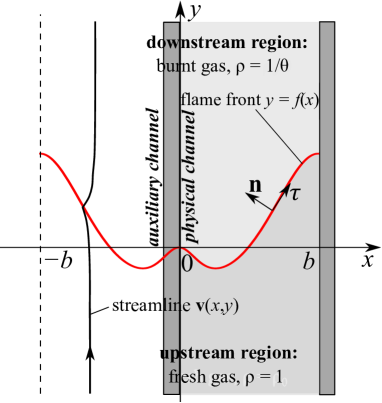
Figure 1: Geometry of steady flame propagation in a straight channel in the rest frame of the flame front

Next, we assume that the flame propagation produces no flow separation at the front endpoints (there is no stagnation in the burnt gas flow). Together with the wall impermeability, this implies the following boundary conditions

$$w(0,y)=w(1,y)=f^{\prime}(0)=f^{\prime}(1)=0,$$ (1)

where prime denotes a derivative with respect to $x$. The on-shell equations take their simplest form under these conditions, because the influence of the channel walls can be simply taken into account by considering the channel flow as a part of an unbounded flow filling the whole $xy$ plane, which is obtained by a periodic continuation of the given flame pattern along the $x$-axis. First, it is mirrored onto an auxiliary channel $x\in[-1,0]$ according to

$$f(x)=f(-x),\quad w(x,y)=-w(-x,y),\quad u(x,y)=u(-x,y).$$ (2)

After that, the flow in the extended channel $x\in[-1,1]$ is periodically continued along the whole $x$-axis. Then the on-shell fresh gas velocity satisfies the following complex integro-differential equation (the master equation) kazakov1 ; jerk2

$$2\omega_{-}^{\prime}+\left(1+\mathrm{i}\hat{\mathcal{H}}\right)\left\{[\omega]^{\prime}-\frac{Nv^{n}_{+}\sigma_{+}\omega_{+}}{v^{2}_{+}}+\frac{1+\mathrm{i}f^{\prime}}{2}\int_{-1}^{+1}\mathrm{d}\xi\;\frac{Nv^{n}_{+}\sigma_{+}\omega_{+}(\xi)}{v^{2}_{+}(\xi)}\right\}=0,$$ (3)

where $\omega=u+\mathrm{i}w$ is the complex velocity and $[\omega]=\omega_{+}-\omega_{-}$ is its jump across the front; the $-(+)$ subscript denotes restriction to the front of a function defined upstream (downstream) of the front, e.g., $w_{-}(x)=w(x,f(x)-0)$; $N=\sqrt{1+f^{\prime 2}}$; $v^{n}_{\pm}={\boldsymbol{v}}_{\pm}\cdot{\boldsymbol{n}}$ is the normal gas velocity (${\boldsymbol{n}}$ being the unit vector normal to the front pointing towards the burnt gas, see Fig. 1), $\sigma=\partial u/\partial x-\partial w/\partial y$ is the gas flow vorticity; finally, the operator $\hat{\mathcal{H}}$ is defined on $2$-periodic functions with zero mean across the channel as

$$\left(\hat{\mathcal{H}}a\right)(x)=\frac{1+\mathrm{i}f^{\prime}(x)}{2}~{}\fint_{-1}^{+1}\mathrm{d}\xi\cot\left\{\frac{\pi}{2}(\xi-x+\mathrm{i}[f(\xi)-f(x)])\right\}\;a(\xi),$$ (4)

with the slash denoting the principal value of the integral.

To complete the system of equations for the three unknown functions $u_{-}(x),w_{-}(x),f(x)$, one has to specify expressions for the normal gas velocity, velocity jumps, and $\sigma_{+}.$ The first one is the so-called evolution equation

$$v_{-}^{n}=1-S(f^{\prime},\omega_{-}),$$ (5)

where $S(f^{\prime},\omega_{-})$ is a quasilocal functional of its arguments that describes the finite-front-thickness effects (the complex velocity is used as an argument of the real $S$ only for brevity; $S$ depends separately on $u_{-}$ and $w_{-},$ as well as on their derivatives). Within the first order in the flame front thickness, it reads

$$S=\mathcal{L}_{\text{c}}\frac{f^{\prime\prime}}{N^{3}}+\mathcal{L}_{\text{s}}\frac{(v_{-}^{\tau})^{\prime}}{N},$$ (6)

where $\mathcal{L}_{\text{c},\text{s}}=O(l_{\text{f}})$ are the parameters (Markstein lengths) quantifying the effects of the flame curvature and its stretch on the local burning rate; $v_{-}^{\tau}\equiv{\boldsymbol{v}}_{-}\cdot{\boldsymbol{\tau}}=(w_{-}+f^{\prime}u_{-})/N$ is the tangential component of the on-shell fresh gas velocity.

Next, the gas velocity jumps follow from the equations (as proved in Ref. kazakov5 , these familiar zero-order relations hold true on inclusion of the first-order finite-front-thickness corrections)

$$v_{+}^{\tau}=v_{-}^{\tau},\quad v_{+}^{n}=\theta v_{-}^{n}$$ (7)

and can be summarized in the expression for the complex velocity jump

$$[\omega]=(\theta-1)\frac{1-\mathrm{i}f^{\prime}}{N}v^{n}_{-}.$$ (8)

Finally, the value of the burnt gas vorticity at the front can be found from the gas pressure jump hayes1957 ; kazakov5

$$\sigma_{+}=[\sigma]=-\frac{1}{Nv_{-}^{n}}\left\{\frac{\theta-1}{2\theta}(v^{\tau}_{-})^{2}+\frac{\theta-1}{2}(v^{n}_{-})^{2}+2\mathcal{L}_{\sigma}\frac{f^{\prime\prime}}{N^{3}}\right\}^{\prime},$$ (9)

wherein $\sigma_{-}=0$ by the Thomson theorem. The constant $\mathcal{L}_{\sigma}$ entering the above expression is the last of the three independent lengths parameterizing the first-order finite-front-thickness effects. The corresponding contribution to $\sigma_{+}$ (or to the pressure jump) describes the so-called flame compression effect (which has nothing to do with the gas compressibility). This term was coined in Ref. class2003 , where importance of the effect with regard to the unstable flame evolution was also alluded. As we show below, it strongly impacts the steady flame structure indeed. $\mathcal{L}_{\sigma}$ is always positive; it vanishes for $\theta\to 1,$ but rapidly grows with $\theta,$ and for flames of practical interest (large $\theta$ and realistic temperature dependence of the kinetic coefficients), $\mathcal{L}_{\sigma}\sim l_{\text{f}}\theta^{3/2}$.

III The numerical scheme

The system in question consists of one complex Eq. (3) [complemented by the jump conditions (8), (9)] and one real Eq. (5). The three unknowns are the $2$-periodic functions $w_{-}(x),u_{-}(x)$, and $f(x),$ obeying reflection conditions (2). It proves useful to combine the real number $u_{-}(0)\equiv u_{0},$ which in what follows will be refereed to as the edge velocity, and the front position into a single (real even) function

$$\varphi(x)=f(x)+u_{0}.$$ (10)

The choice $f(0)=0$ implies that $u_{0},f$ can be expressed via $\varphi$ as $u_{0}=\varphi(0)$, $f(x)=\varphi(x)-\varphi(0)$.

The iterative procedure we use for numerical solving of the system is as follows. Consider an approximation $\varphi^{(p)}(x)$ of $\varphi^{\star}(x),$ which is part of the solution $\bigl{(}w_{-}^{\star}(x),u_{-}^{\star}(x),\varphi^{\star}(x)\bigr{)}$ of the system. With a fixed $\varphi=\varphi^{(p)}$, the master equation (3) is a nonlinear integro-differential equation for the function $\omega_{-}(x)$. Its solutions can be found as fixed points of a recurrence relation

$$\omega_{-}^{(m+1)}(x)=u_{0}+\int_{0}^{x}\mathrm{d}\xi\;K[\omega_{-}^{(m)},\varphi](\xi),\qquad m=0,1,2,\ldots,$$ (11)

where $K$ is the nonlinear integro-differential operator determining $\omega_{-}^{\prime}$ according to Eq. (3). Actual simulations show that iterations (11) rapidly converge to a unique solution $\omega_{-}^{\star}[\varphi]$ for any reasonable function $\varphi(x)$ and iteration seed $\omega_{-}^{(0)}(x)$. After that, to construct a new approximation $\varphi^{(p+1)}(x)$ of $\varphi^{\star}(x)$ (that is, a new $f^{(p+1)}(x)$ and a new $u^{(p+1)}_{0}$), we use the evolution equation (5) written as

$$v_{-}^{n(p+1)}=1-S\bigl{(}f^{(p+1)}{}^{\prime},\;\omega_{-}^{\star}[\varphi^{(p)}]+u_{0}^{(p+1)}-u_{0}^{(p)}\bigr{)},$$ (12)

with the left-hand side understood as

$$v_{-}^{n(p+1)}=\frac{u_{-}^{\star}[\varphi^{(p)}]+u_{0}^{(p+1)}-u_{0}^{(p)}-f^{(p+1)}{}^{\prime}w_{-}^{\star}[\varphi^{(p)}]}{\sqrt{1+f^{(p+1)}{}^{\prime}\,{}^{2}}}.$$ (13)

Note that $\omega_{-}^{\star}[\varphi^{(p)}]$ enters the above equations in a ‘corrected’ form: it is shifted by $(u_{0}^{(p+1)}-u_{0}^{(p)})$ in order to match the edge velocity of the next (unknown) iteration. $f^{(p+1)}(x)$ is the solution of the ordinary differential equation (12). Together with the boundary conditions at the channel walls, this equation constitutes an overdetermined system, and therefore, implies a condition on the iterated edge velocity $u_{0}^{(p+1)}$. In fact, a first-order ordinary differential equation (12) in its unknown $f^{(p+1)}{}^{\prime}(x)$ is to be solved with two boundary conditions $f^{(p+1)}{}^{\prime}(0)=f^{(p+1)}{}^{\prime}(1)=0$. Such a system may have solutions only for special values of $u_{0}^{(p+1)}$. Indeed, if we integrate it with the initial condition $f^{(p+1)}{}^{\prime}(0)=0$, then the other condition yields an algebraic equation for $u_{0}^{(p+1)}$

$$f^{(p+1)}{}^{\prime}[\omega_{-}^{\star}[\varphi^{(p)}],u_{0}^{(p+1)}](1)=0.$$ (14)

Thus, in this computational scheme, $u_{0}$ plays the role of eigenvalue. Its approximation $u_{0}^{(p+1)}$ is found by scanning a vicinity of $u_{0}^{(p)},$ that is, by solving Eq. (12) with different $u_{0}^{(p+1)}$ until condition (14) is met (a technique for solving boundary-value problems usually referred to as the shooting method). Note also that for actual flames, shooting can be done efficiently using bisections, since the left-hand side of Eq. (14) turns out to be a monotonic function of $u_{0}^{(p+1)}$. After the latter is found, the corresponding $\varphi^{(p+1)}$ can be evaluated as

$$\varphi^{(p+1)}(x)=u_{0}^{(p+1)}+\int_{0}^{x}\mathrm{d}\xi\;f^{(p+1)}{}^{\prime}[\omega_{-}^{\star}[\varphi^{(p)}],u_{0}^{(p+1)}](\xi)\equiv\mathcal{I}[\varphi^{(p)}](x).$$ (15)

We conclude that if the described iterative procedure converges, the sought-after solution $\bigl{(}w_{-}^{\star},u_{-}^{\star},\varphi^{\star}\bigr{)}$ can be found as $\bigl{(}w_{-}^{\star}[\varphi^{\star}],u_{-}^{\star}[\varphi^{\star}],\varphi^{\star}\bigr{)}$, where $\varphi^{\star}$ is a fixed point of the map (15),

$$\mathcal{I}[\varphi^{\star}]=\varphi^{\star}.$$ (16)

The fixed point $\varphi^{\star}$ does not necessarily have to be reached using simple iterations (the Picard method), i.e., by repeated application of $\mathcal{I}$ to some seed $\varphi^{(0)}$. For instance, one can introduce a weight $\beta\in(0,1]$ to redefine the iteration as

$$\varphi_{p+1}=(1-\beta)\varphi_{p}+\beta\mathcal{I}[\varphi_{p}],$$ (17)

so that $\varphi^{\star}$ is also a fixed point of the modified recurrence relation. As is well known, both conventional and weighted iterations converge in a sufficiently small vicinity of the fixed point, provided that $\mathcal{I}$ is a contraction at this point, i.e., $\|\mathcal{I}[\varphi]-\varphi^{\star}\|<\lambda\|\varphi-\varphi^{\star}\|$ for some $\lambda\in(0,1)$ and $\varphi\to\varphi^{\star}$ Olshansky_IterativeMethods . In the present case, however, this condition turns out to be a too severe limitation, because not all of the fixed points happen to correspond to contracting operators $\mathcal{I}$.

There exist a number of techniques to overcome this difficulty. A notable one is the Anderson acceleration method Anderson , which is virtually a generalization of the Krylov subspace approaches to nonlinear equations Olshansky_IterativeMethods . In this method, the $(p+1)$th approximation is constructed as a weighted average of $d\geq 1$ preceding iterates

$$\varphi_{p+1}=\alpha_{p,1}\varphi_{p}+\alpha_{p,2}\varphi_{p-1}+\ldots+\alpha_{p,d}\varphi_{p-d+1},\qquad\alpha_{p,k}\in\mathds{R},\qquad\sum\limits_{k=1}^{d}\alpha_{p,k}=1,$$ (18)

the weights $\alpha_{p,1},\ldots,\alpha_{p,d}$ being chosen so as to minimize the Euclidean norm of the residual $\epsilon_{p+1}=\mathcal{I}[\varphi_{p+1}]-\varphi_{p+1}$. Under the assumption that the iterates are sufficiently close to the fixed point $\varphi^{\star}$ [and hence so is $\varphi_{p+1}$, by virtue of Eq. (18)], $\mathcal{I}$ can be linearized, and the residual norm squared can be written as a quadratic form

$$\epsilon_{p+1} \equiv \mathcal{I}[\varphi_{p+1}]-\varphi_{p+1}\approx\mathcal{I}[\varphi^{\star}]+\mathcal{I}^{\prime}[\varphi^{\star}](\varphi_{p+1}-\varphi^{\star})-\varphi_{p+1}\equiv\mathcal{J}\cdot(\varphi_{p+1}-\varphi^{\star}),\quad\mathcal{J}\equiv\mathcal{I}^{\prime}[\varphi^{\star}]-1,$$ (19)

$$\|\epsilon_{p+1}\|^{2} \approx \|\mathcal{J}(\varphi_{p+1}-\varphi^{\star})\|^{2}=\left\|\sum_{k=1}^{d}\alpha_{p,k}\mathcal{J}(\varphi_{p-k+1}-\varphi^{\star})\right\|^{2}=\sum_{k,l=1}^{d}g_{kl}^{(p)}\alpha_{p,k}\alpha_{p,l}.$$ (20)

The coefficients of this quadratic form can be evaluated by computing the scalar products of the residuals, $g_{kl}^{(p)}=(\epsilon_{p-k+1},\epsilon_{p-l+1})$. Minimization of the residual then reduces to the well-known linear least-squares (LLS) problem, i.e., to minimization of the quadratic form (20) with respect to its arguments $\alpha_{p,1},\ldots,\alpha_{p,d-1}$, the last argument $\alpha_{p,d}=1-\sum_{k=1}^{d-1}\alpha_{p,k}$ being a linear function of the others (see, e.g., LeastSquares ). Not only does the Anderson method permit searching for non-contracting fixed points, it is also more robust than simple iterations: if, for some reason, the $p$th iteration step has thrown $\varphi_{p+1}$ away of the fixed point, the residual minimization will suppress the weight of the ‘bad solution’ $\varphi_{p+1}$ in subsequent iterates, so that one ‘bad try’ will not spoil the whole iterative sequence. Moreover, linear constraints on $\varphi$ are readily incorporated into the Anderson method. For example, the edge velocity constraint $\xi_{-}\leq u_{0}\equiv\varphi(0)\leq\xi_{+}$ leads to a linear inequality-constrained least-squared (CLS) problem on the weights $\alpha_{p,k}$, which admits an explicit solution similar to the one for LLS LeastSquares . In our simulations, we use this constraint for separating different solution branches.

It is worth mentioning that the slowest part of the computation, namely, the integral transform (4) requiring $\mathit{O}(N^{2})$ operations for $N$ grid points across the channel, is readily parallelized, since the values of the transform at different points can be evaluated independently. To give an idea of the efficiency of the algorithm, we mention that most of the results presented below were obtained on a dual-core Intel Atom D525 1.7GHz machine, where it takes about one minute to find a solution for a grid with $N=1000$ and flame slope tolerance of $5\times 10^{-3}$; we resorted to single-node multiprocessor computation on a supercomputer only for large series of solutions (about 250) needed to build a three-dimensional plot. Further technical details of the numerical approach implemented in our solver, including evaluation of the singular-kernel integral transform (4), the use of non-uniform grids, regularization of the inverse matrices $g^{(p)\,{-1}}$ necessary for the CLS/LLS minimizations, etc., will be given elsewhere OKKK_FlameSolver .

IV The applications

The developed method will now be used to study various effects that control formation of steady flames. In contrast to DNS or real experiments where all the parameters $\theta,$ $\mathcal{L}_{\text{c},\text{s},\sigma}$ have fixed values specific to the given mixture, our approach allows separate investigation of the effects by varying one of the parameters while keeping the others fixed. We first set $\mathcal{L}_{\text{s}}=\mathcal{L}_{\sigma}=0$ to consider the most common mechanism of flame stabilization by the front curvature effect at several representative values of $\theta.$ This helps to illustrate critical importance of the gas expansion parameter which is often depreciated in the theoretical combustion. Nonzero $\mathcal{L}_{\text{s}},\mathcal{L}_{\sigma}$ are then included to investigate the flame stretch and compression, to infer an interesting interplay between different effects, and to establish an important universality of the dependence of the flame speed on the channel width. In general, there exist several solutions for each point $(\theta,\mathcal{L}_{\text{c}},\mathcal{L}_{\text{s}},\mathcal{L}_{\sigma})$ of the parameter space, but for the sake of brevity, we present only the one maximizing the flame propagation speed $U.$ Though proved only within the weakly-nonlinear theory vaynblat , it seems to be in the nature of free flame evolution that only such solutions can be stable against small perturbations.

IV.1 The effect of finite gas expansion. A practical limitation of the weak-nonlinearity analysis

Steady flame formation in a channel can be described as a nonlinear stabilization of a finite number of unstable modes, which grow and gradually coalesce into larger and more slowly evolving patterns. In the regime of saturated nonlinearity, the front slope is not small over most part of the flame unless $(\theta-1)\equiv\alpha$ is small. But since it drops down to zero near the channel walls (by virtue of the boundary conditions existing thereat), the walls appear to exert a stabilizing effect on the flame. This gives hope that the weakly-nonlinear theory could be applicable even to flames with non-small $\alpha$ in sufficiently narrow channels. However, the downside of this stabilization is a non-uniformity of the gas velocity distribution across the channel. Namely, to meet the conditions $w=0,$ $f^{\prime}=0,$ the flow variables have to rapidly vary near the wall (this happens normally at the trailing edge of the flame), which results in an enhanced vorticity production in this region. This is illustrated by Fig. 2 showing the front shapes and on-shell vorticities of the burnt gases for flames with $\theta=1.5,3$, and $5$ propagating in a channel of width $b=0.75\lambda_{\text{c}}.$ We observe that despite the seemingly smooth front shapes, vorticity is sharply peaked near the wall $x=b,$ significantly exceeding unity (in natural units) already for such a moderate gas expansion as $\theta=3.$ At the same time, the small-$(\theta-1)$ expansion implies smallness of the burnt gas vorticity: once the flame-induced gas velocity variations $\Delta u,\Delta w$ are assumed to be much less than unity, so must be their derivatives, because $\lambda_{\text{c}}$ and $b$ are the only characteristic lengths in this approach, and in the case $\lambda_{\text{c}}\simeq b=1$ one has, e.g., $u_{+}^{\prime}\simeq\Delta u/\lambda_{\text{c}}\simeq\Delta u\ll 1$ (in fact, the small-$(\theta-1)$ expansion assumes that differentiation of a flow variable raises its smallness order by one; the key points of this expansion are summarized in the Appendix). We thus see that the assumption of weak vorticity production is not valid for flames with $\alpha\gtrsim 1$ even in narrow channels. As is evident from the figure, an underlying reason is that for such flames $\lambda_{\text{c}}$ is not actually the smallest characteristic length: the burnt gas vorticity varies on a much smaller scale $\approx\mathcal{L}_{\text{c}}$.

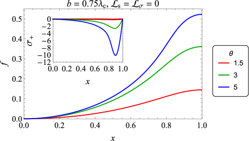
Figure 2: Front position and burnt gas vorticity distribution at the front (inset) for flames with $\theta=1.5,\mathcal{L}_{\text{c}}=0.036$ (red lines), $\theta=3,\mathcal{L}_{\text{c}}=0.072$ (green lines), and $\theta=5,\mathcal{L}_{\text{c}}=0.086$ (blue lines); channel width $b=0.75\lambda_{\text{c}}$ in all cases.

Still, one might think that this breakdown of the basic assumption is not very important because it is confined to a comparatively narrow layer near the wall. That this is not so is clearly seen from the plots of the flame propagation speed versus $\lambda_{\text{c}}$, Fig. 3. Comparison with the theoretical results (dashed lines) reveals significant deviations from the characteristic ‘arch’ structure, predicted by the weakly-nonlinear theory, which rapidly grow with $\theta.$ Being proportional to the total front length, the flame speed would deviate by an amount $\sim\mathcal{L}_{\text{c}}/b\ll 1$ if the vorticity peak affected the front shape only near the wall. Therefore, the greater deviations exposed by Fig. 3 mean that what is happening near the walls actually affects the whole flame. This conclusion is not unexpected in such an essentially nonlocal problem as the slow flame propagation. The interaction between distant regions of the front ceases only in the case of highly elongated flames, such as those formed by a strong gravity kazakov3 ; kazakov4 . It can be added that for still larger values of the gas expansion parameter, the burnt gas vorticity significantly exceeds unity also at distances $\sim b$ away from the walls, that is, virtually all over the flame front except near the vorticity nodes. In the case shown in Fig. 4, for instance, the vorticity magnitude averaged over the front is approximately $11$.

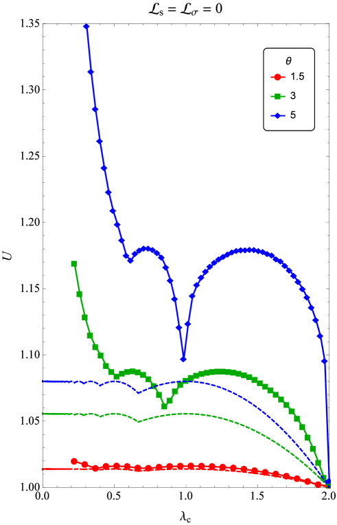
Figure 3: Flame speed versus the cutoff wavelength for flames with $\theta=1.5,3,\text{ and }5$ (solid red, green, and blue lines, respectively). $\mathcal{L}_{\text{s}}=\mathcal{L}_{\sigma}=0$ in all cases. The corresponding predictions of the weakly-nonlinear theory (solutions of the Sivashinsky-Clavin equation sivclav ) are shown by dashed lines.

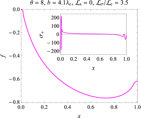
Figure 4: Front position and burnt gas vorticity distribution at the front (inset) for a flame with $\theta=8,$ $\mathcal{L}_{\text{c}}=0.031$ propagating in a channel of width $b=4.1\lambda_{\text{c}}$.

Curiously, the pole solutions to the Sivashinsky–Clavin equation, when applied to flames with $\theta-1\gtrsim 1,$ qualitatively correctly reproduce the singular behavior of vorticity near one of the walls, if it is calculated by substituting Eqs. (5), (26) into Eq. (9), see Fig. 5. Of course, the small-scale structure occurs in this case because the small length $\mathcal{L}_{\text{c}}$ is explicitly present in the expression for the vorticity. The fact that the weakly-nonlinear theory predicts this behavior of vorticity, but fails at the same time to take into account its effect on the flame structure is an indirect but quite a vivid demonstration of impossibility to apply this theory to flames with arbitrary $\theta$ (a more direct demonstration can be found in Ref. kazakov6 ).

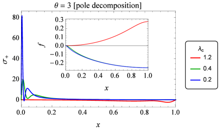
Figure 5: Burnt gas vorticity at the front as given by the pole solutions (29)–(31) of Eq. (27) for flames with $\theta=3$ and various cutoff wavelengths: $\lambda_{\text{c}}=1.2$ (red line), $\lambda_{\text{c}}=0.4$ (green line), and $\lambda_{\text{c}}=0.2$ (blue line). Inset: the corresponding front positions.

It should be noted that not only peculiarities in the vorticity production, but also major manifestations of the finite-front-thickness effects are confined to the near-wall layers. This is well illustrated by the normal flame speed plots in Fig. 6. The normal speed is seen to be remarkably constant across the channel except at distances $O(\mathcal{L}_{\text{c}})$ from the walls, and the more close it is to unity, the less is $\mathcal{L}_{\text{c}}$. Thus, nonlinear stabilization of flames with non-small $\alpha$ acts so as to reduce as much as possible the flame front curvature and flow strain in the bulk at the cost of their enhancement near the front ends (this conclusion holds true on inclusion of the flame stretch and compression terms).

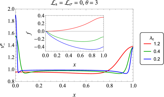
Figure 6: Normal speed of flames with $\lambda_{\text{c}}=1.2$ ($\mathcal{L}_{\text{c}}=0.064$, red line), $\lambda_{\text{c}}=0.4$ ($\mathcal{L}_{\text{c}}=0.021$, green line), and $\lambda_{\text{c}}=0.2$ ($\mathcal{L}_{\text{c}}=0.011$, blue line). Inset: the corresponding front positions. In all the plots, $\theta=3$ and $\mathcal{L}_{\text{s}}=\mathcal{L}_{\sigma}=0$.

For generic values of the Markstein parameters, enhanced vorticity production near the walls ceases only for sufficiently small $\alpha.$ As our results show, the position and height of the two rightmost arches of the flame speed curves (which correspond to $b\lesssim 2.5\lambda_{\text{c}}$) are described by the pole solutions reasonably well for $\alpha\lesssim 0.5$. Restriction $\theta\lesssim 1.5$ is thus a practical limitation of applicability of the weakly-nonlinear theory in narrow channels. Yet, even for such $\theta$’s, deviations from the predictions of this theory grow rapidly with the channel width starting from $b\approx 3\lambda_{\text{c}},$ as further discussed in Sec. IV.4.

IV.2 The flame stretch effect

It is common for theoretical as well as experimental flame studies not to distinguish the flame curvature and stretch contributions to the normal flame speed, despite the fact that in general the two effects are quite different. There are several reasons for that. One is that the two contributions take on the same functional form for nearly planar flames. In the weakly-nonlinear theory, the corresponding Markstein lengths enter the equation for the front position through a single parameter, the cutoff wavelength [cf. Eqs. (27), (28)]. It is thus often believed that specifying the value of this parameter is sufficient for a global flame description. Another reason is the well-known result matalon1982 of asymptotic analysis of the inner flame structure that in the simplest case of a one-step reaction with high activation energy, only the stretch contributes to the normal flame speed when the discontinuity surface replacing the front is identified with the reaction zone. Only recently was it understood kazakov5 that such an identification is not self-consistent, and theoretical investigation of more realistic models has begun clavin2011 . On the experimental side, accuracy of the standard flame speed measurements usually does not allow separation of the stretch and curvature contributions, so that one length parameter turns out to be sufficient to fit the experimental data.

Our results confirm that varying the ratio of the parameters $\mathcal{L}_{\text{c}},\mathcal{L}_{\text{s}}$ keeping $\lambda_{\text{c}}$ fixed does not significantly change the flame structure. Examples are given in Figs. 7(a)–7(c), 8 which contain plots of the flame front position, on-shell gas velocity and burnt gas vorticity for three different pairs $\mathcal{L}_{\text{c}},\mathcal{L}_{\text{s}}$, all having the same $\lambda_{\text{c}}.$ Still, there is an important trend produced by the flame stretch and revealed by the flame speed curves in Fig. 7(d), namely, that the flame propagation speed increases as $\mathcal{L}_{\text{s}}$ decreases, except near the dips on the curves (e.g., $\lambda_{\text{c}}\approx 0.9$). In this regard, things are the same as in gravity-driven flame propagation [according to the experimental evidence levy1965 and calculations kazakov5 , propane-air flames ($\mathcal{L}_{\text{s}}>0$) propagate somewhat slower in the lean limit than methane-air flames ($\mathcal{L}_{\text{s}}<0$)].

$\begin{array}[]{cc}\includegraphics[height=170.71652pt]{fig7a.eps}&\includegraphics[height=170.71652pt]{fig7b.eps}\\ \text{(a)}&\text{(b)}\\ \includegraphics[height=170.71652pt]{fig7c.eps}&\includegraphics[height=170.71652pt]{fig7d.eps}\\ \text{(c)}&\text{(d)}\end{array}$

Figure 7: Flame front position (a), gas velocities $u_{-}$ (solid lines), $w_{-}$ (dashed lines) (b), and burnt gas vorticity (c) for $\lambda_{\text{c}}=0.4,\theta=3$ and $\mathcal{L}_{\text{s}}=\mathcal{L}_{\text{c}}$ (red lines), $\mathcal{L}_{\text{s}}=0$ (green lines), $\mathcal{L}_{\text{s}}=-\mathcal{L}_{\text{c}}/4$ (blue lines); inset: the corresponding normal (solid lines) and tangential (dashed lines) fresh gas velocities. (d) Flame propagation speed versus $\lambda_{\text{c}}$ for the same $\mathcal{L}_{\text{s}}$’s.

$\begin{array}[]{cc}\includegraphics[height=170.71652pt]{fig8a.eps}&\includegraphics[height=170.71652pt]{fig8b.eps}\\ \text{(a)}&\text{(b)}\end{array}$ $\begin{array}[]{c}\includegraphics[height=170.71652pt]{fig8c.eps}\\ \text{(c)}\end{array}$

Figure 8: Same as in Figs. 7(a)–7(c), but for $\lambda_{\text{c}}=0.2$.

IV.3 The flame compression effect

Unlike the finite-front-thickness corrections to the normal flame speed, the effect of flame compression on the flame structure remains virtually unexplored. This is because the normal flame speed is directly measurable, and the result (6) of calculations can be readily compared with experiment. It is also important that similar verifications can be made in situations where the weakly-nonlinear theory applies, such as those found in studies of various instabilities of nearly planar flames markstein1951 ; barenblatt1962 ; searby1991 . In contrast, the flame compression manifests itself in the gas-pressure jump at the front, hence affects only vorticity production by the flame, but not the gas-velocity jumps themselves. In the weakly-nonlinear Sivashinsky theory siv , the burnt gas vorticity is neglected completely, while in the next approximation sivclav it is considered small. As a result, in theories based on the small $(\theta-1)$ expansion, all the three Markstein lengths $\mathcal{L}_{\text{c}},\mathcal{L}_{\text{s}}$, and $\mathcal{L}_{\sigma}$ combine into a single parameter – the cutoff wavelength of unstable flame perturbations, $\lambda_{\text{c}}$ [cf. Eq. (28) in Appendix]. Thus, although the flame compression does change $\lambda_{\text{c}}$, its effect is masked by those of the flame stretch and curvature. For this reason, any qualitatively new effect associated with the flame compression will be essentially non-perturbative. As the obtained numerical solutions show, this is the case indeed. The flame compression turns out to have a rather nontrivial impact on the structure of steady flames with finite $\theta,$ which is not captured by the small $(\theta-1)$ expansion and is closely related to the enhanced vorticity production near the channel walls, discussed in Sec. IV.1.

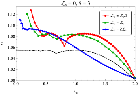
Figure 9: Flame speed versus the cutoff wavelength $\lambda_{\text{c}}$ for $\theta=3$ and various $\mathcal{L}_{\sigma}/\mathcal{L}_{\text{c}}$ ratios ($\mathcal{L}_{\text{s}}=0$ throughout). Red, green, and blue curves correspond to $\mathcal{L}_{\sigma}/\mathcal{L}_{\text{c}}=0.5,1,2$, respectively (the green curve realizes condition (21)). Dashed curve represents solutions of the Sivashinsky–Clavin equation.

According to Eq. (28), contribution of the flame compression to the cutoff wavelength is negative. This means that during the initial development of Darrieus–Landau instability, flame compression additionally destabilizes the flame, hence, strengthens the flow nonlinearity. It is therefore somewhat surprising that in a certain range of parameters, inclusion of this effect improves applicability of the weakly-nonlinear theory. Namely, a series of the flame velocity curves in Fig. 9 demonstrate that as $\mathcal{L}_{\sigma}$ increases from zero to values of the order of $\mathcal{L}_{\text{c}},$ solutions of the exact system first tend to follow more closely the pole solutions. In particular, locations of the dips on the flame speed curve shift towards the points $b/\lambda_{\text{c}}=n+1/2,$ $n=1,2,...,$ which correspond to the appearance of new poles in the pole decomposition [cf. Eq. (32)]. However, as $\mathcal{L}_{\sigma}$ increases further, deviations from the weakly-nonlinear theory begin to grow, and the flame speed versus $\lambda_{\text{c}}/b$ ultimately becomes entirely different from the arch-shaped curve obtained using the small-$(\theta-1)$ expansion. This behavior is readily understood once we observe that when the Markstein lengths $\mathcal{L}_{\text{c},\sigma}$ are related by

$$\mathcal{L}_{\sigma}=\frac{\alpha}{2}\mathcal{L}_{\text{c}},$$ (21)

the flame compression contribution to the vorticity jump (9) exactly cancels the curvature contribution coming from the term $(v^{n}_{-})^{\prime}.$ The higher-derivative terms, which are most sensitive to rapid variations of the front slope, thus disappear from $\sigma_{+}.$ As a consequence, the near-wall peaks in the vorticity production become smoothed, and the agreement with the weakly-nonlinear theory improves. This is illustrated by the vorticity plots in Fig. 10. It is seen that inclusion of the flame compression with $\mathcal{L}_{\sigma}=0.5\mathcal{L}_{\text{c}}$ reduces the vorticity peak near the wall $x=0$ from $\sigma_{+}\approx 15$ [Cf. Fig. 7(c)] to $\sigma_{+}\approx 6.$ It is further damped and split into two peaks of opposite signs with $|\sigma_{+}|\approx 1$ in the case $\mathcal{L}_{\sigma}=\mathcal{L}_{\text{c}}$ that fulfills condition (21). The integral effect of the vorticity production near the wall on the global flame structure is also reduced by the peak alternation. At last, a still larger $\mathcal{L}_{\sigma}$ leads to the appearance of a positive vorticity peak $\sigma_{+}\approx 22$ near the wall $x=1$ in place of the negative peak $\sigma_{+}\approx-9$ that existed for $\mathcal{L}_{\sigma}=0.$

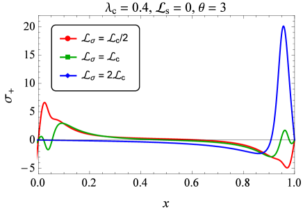
Figure 10: On-shell burnt gas vorticity in flames with $\theta=3,$ $\lambda_{\text{c}}=0.4,$ $\mathcal{L}_{\text{s}}=0$ and $\mathcal{L}_{\sigma}=0.5\mathcal{L}_{\text{c}}$ (red line), $\mathcal{L}_{\sigma}=\mathcal{L}_{\text{c}}$ (green line), $\mathcal{L}_{\sigma}=2\mathcal{L}_{\text{c}}$ (blue line).

IV.4 The flame speed rise and the role of noise

The theory based on the weak-nonlinearity assumption predicts that the steady flame propagation speed tends to a constant value as the channel width increases [cf. Eqs. (33), (34) and Fig. 14 of Appendix]. However, it is well known from the experiment that the flame speed strongly increases with $b.$ At the same time, any laboratory flame can be considered steady only with a certain degree of accuracy, because of various uncontrollable factors such as small mixture inhomogeneities or turbulent motions developing in the fast burnt gas outflow. Similarly, DNS show a strong rise of the flame speed starting from some critical $b,$ but it is difficult to obtain a truly steady flame in sufficiently wide computational domains: the errors caused by the numerical roundoff, finiteness of the domain lateral extent, etc.produce small perturbations of the flame which can grow large before they are carried away downstream, and thus lead to a noticeable increase in the flame speed or even trigger transitions between different propagation regimes. It was, therefore, suggested that these flow irregularities, or noise, are the reason for the discrepancy between the theory and observations procaccia1997 ; procaccia1998 ; almarcha2015 . Specifically, it was shown in Refs. procaccia1997 ; procaccia1998 that by introducing a noise term into the Sivashinsky equation and choosing appropriately the noise spectrum and intensity, one can obtain the flame speed scaling with the channel width as $U\sim b^{\mu},$ where $\mu$ can take on different values, e.g., $0.35,0.42$, and even $\mu>1.5$.

It is true that the noise is present in the real experiment as well as in simulations, and there is little doubt that the flame speed can be raised to the observed values by taking the noise magnitude sufficiently large. But before declaring the noise responsible for the found discrepancies, it is worth exploring the possibility that the flame speed rise is a steady-flame phenomenon which is essentially non-perturbative, in that it is not captured by the weak-nonlinearity treatment. The master equation (3) is a perfect means for this purpose: being time-independent by construction, it is free of the unsteady phenomena caused by the noise, and being an exact consequence of the fundamental gasdynamic equations, it takes full account of the flow nonlinearities generated by a steady flame.

In the flame speed plots presented above, the speed is seen to steeply rise to the left of the second dip, which in the pole-decomposition picture corresponds to $b=(2+1/2)\lambda_{\text{c}}.$ To see how this compares with the known behavior of unsteady flames, we use the DNS results of Ref. Liberman . To identify the region in the parameter space that corresponds to the conditions of Ref. Liberman we take into account that these DNS were carried out in the case of unit Lewis number, Prandtl number equal to 0.5, temperature-independent thermal conductivity, and the reduced activation energy of a one-step chemical reaction equal to 7. The latter comparatively large value suggests to adopt the thin reaction zone approximation, within which the Markstein lengths for the specified values of Lewis and Prandtl numbers read (explicit expressions given in Ref. class2003 are valid for the gas thermal conductivity scaling as the square root of temperature; in the case of interest, expressions (22) can be obtained from the general formulas (3.32)–(4.20) of Ref. class2003 )

$$\mathcal{L}_{\text{c}}=\frac{\theta\ln\theta}{\theta-1}l_{\text{f}},\quad\mathcal{L}_{\text{s}}=0,\quad\mathcal{L}_{\sigma}=\frac{\theta\ln\theta}{2}l_{\text{f}}.$$ (22)

It is easy to check a curious fact that these lengths fulfill condition (21). Our results for the flame speed versus cutoff wavelength are compared with the DNS data in Figs. 11, 12. Although the values (22) pertain to the limit of infinite activation energy, so that agreement with the DNS can be improved by varying Markstein parameters around these values, the comparison leaves no doubt that the two datasets describe the same flame-speed behavior, in particular, the same phenomenon of the flame speed rise at small $\lambda_{\text{c}}$. The piece of the DNS data describing this rise is shown in Fig. 11 as a dashed line because of a significant scatter in the data caused by numerical noise. Since there is no such problem with the steady on-shell solutions, we conclude that the speed rise at small $\lambda_{\text{c}}$ is not related to noise or some flame instability, but is an intrinsic property of steady flames.

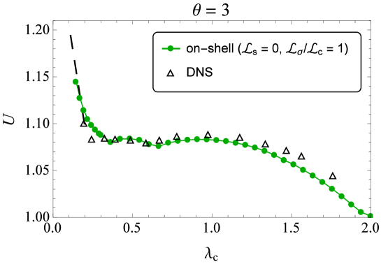
Figure 11: Propagation speed of flames with $\theta=3$ versus the cutoff wavelength as given by the on-shell solutions with Markstein lengths (22) (circles), and by DNS Liberman (triangles).

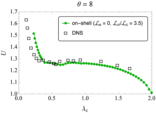
Figure 12: Same as in Fig. 11, but for $\theta=8$.

To demonstrate that the found flame speed rise is quite universal, not just specific to the particular choice (22) of Markstein lengths, we present in Fig. 13 a three-dimensional plot of the flame speed as a function of two independent parameters $\mathcal{L}_{\text{c}}$ and $\mathcal{L}_{\text{s}}.$ For sufficiently small values of $\mathcal{L}_{\sigma}$ [such as the one given by Eq. (21), or less], the threshold of the speed rise is $b\approx 2\lambda_{\text{c}}\div 3\lambda_{\text{c}},$ but it noticeably grows with $\mathcal{L}_{\sigma}$ [Cf. the case $\mathcal{L}_{\sigma}=2\mathcal{L}_{\text{c}}$ in Fig.9 where it is $\approx 12\lambda_{\text{c}}$]. On the other hand, the threshold value turns out to be much less sensitive to the flame compression when expressed in terms of the curvature and stretch Markstein lengths. For $\mathcal{L}_{\text{s}}=0,$ for instance, it is $b\approx 35\mathcal{L}_{\text{c}}$ almost regardless of $\mathcal{L}_{\sigma}$.

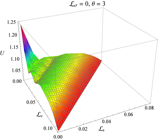
Figure 13: Propagation speed of flames with $\theta=3$ as a function of $\mathcal{L}_{\text{c}},\mathcal{L}_{\text{s}}$.

V Conclusions

The on-shell description of flame propagation makes it unnecessary to resolve the flow structure in the streamwise direction. This dimensional reduction of the problem gives a great advantage over conventional methods based on direct solution of the fundamental gasdynamic equations. We have shown that the system of the on-shell equations for a steady flame can be solved numerically in a comparatively simple way using two-level nested fixed-point iterations. Inner iterations give a solution of the master equation for a fixed, current flame front position, which is then used to construct a subsequent outer iteration of the flame front itself – namely, to solve the evolution equation for the obtained gas velocity distribution along it.

Another important advantage over experimental studies and DNS is that our approach permits separate investigation of various effects controlling the flame evolution. The results of such an investigation of the channel flame propagation, carried out in Sec. IV, lead us to the following main conclusions:

• As a result of nonlinear flame stabilization in a channel, layers near the channel walls develop, which are characterized by an enhanced vorticity production and large flame front curvature. Markstein length $\mathcal{L}_{\text{c}}$ is the characteristic length of the flow fields in these layers, wherein the magnitudes of the vorticity and front curvature strongly grow with the gas expansion coefficient $\theta$. The existence of these layers makes the weakly-nonlinear theory inapplicable to flames with $\theta-1\gtrsim 1$ even in narrow channels.

• Flame compression significantly affects the flame structure by modifying the vorticity production in the flame. This modification is especially pronounced in the same near-wall layers in which rapid variations of the flow variables take place. In particular, the flame compression violently alters the dependence of the flame propagation speed on the channel width, so that the usual ‘arch’-shaped profile predicted by the weakly-nonlinear theory turns out to be smoothed and nearly monotonic for sufficiently large $\mathcal{L}_{\sigma}$.

• A steep rise of the flame propagation speed observed in sufficiently wide channels is a steady flame phenomenon up to at least $b=200\mathcal{L}_{\text{c}}$. It has nothing to do with noise or any other possible flame unsteadiness that can be present in DNS or an actual experiment.

These observations in turn raise an important and quite nontrivial question of an ultimate structure of the near-wall layers in the limit $b/\lambda_{\text{c}}\to\infty$. Since the magnitude of the vorticity peaks grows (apparently, without bound) as $b$ increases, it is clear that either the inner flame structure or the structure of the gas flow in these layers must eventually change so as to keep the vorticity bounded. Our results show that as $b$ increases, the front slope becomes very large just before it drops down to zero at the channel wall, that is, the front turns out to be nearly parallel to the wall. This suggests that the required change in the inner flame structure might be its local quenching. Formulated as the vanishing normal velocity $v^{n}_{-}$ at the wall, this would also align the front with the wall, but eliminate the undesirable large front curvature. Another option – a change in the outer flow structure – can be realized through the formation of a stagnation zone in the burnt gas flow. This would lift condition $f^{\prime}=0$ at the wall, and hence relax the flow strain in the near-wall layers. Hopefully, resolution of this question will help to identify the boundary conditions relevant to the flame propagation in situations where the flame propagation speed largely exceeds its normal speed.

Appendix A Equation for the front position in the first post-Sivashinsky approximation

In this appendix, we derive an equation for the flame front position in the first post-Sivashinsky approximation (a steady version of the Sivashinsky–Clavin equation sivclav ) taking into account the flame compression effect. This is primarily to recapitulate the main assumptions underlying the weak-nonlinearity analysis, and to recall basic properties of the pole decomposition solutions thual1985 .

Soon after the onset of the planar flame instability, the cutoff wavelength of unstable flame perturbations, $\lambda_{\text{c}},$ becomes the smallest characteristic length of the weakly curved flame, because perturbations with wavelengths smaller than $\lambda_{\text{c}}$ rapidly die out during the linear stage of Darrieus–Landau instability. A starting point of the small-$(\theta-1)$ expansion is the fact of the linear stability analysis that $\lambda_{\text{c}}\sim l_{\text{f}}/(\theta-1).$ This suggests that for a given front thickness $l_{\text{f}}$, any flame pattern will be “stretched out” in the $x$-direction as $\theta\to 1$. In other words, assuming that $\lambda_{\text{c}}$ remains the smallest length during the subsequent flame evolution, the flame nonlinearity can be made weak by choosing $(\theta-1)$ sufficiently small. $(\theta-1)\equiv\alpha$ thus becomes a small parameter of the weak-nonlinearity expansion. Since $\lambda_{\text{c}}=O(1/\alpha)$, the $x$-differentiation of an on-shell quantity raises its smallness order within this expansion by one. For instance, the front slope is to be treated as a first-order quantity, $f^{\prime}=O(\alpha),$ whereas $f^{\prime\prime}=O(\alpha^{2}).$ Similarly, $w^{\prime}=O(\alpha w),$ $u^{\prime}=O(\alpha(u-1)).$

The first post-Sivashinsky approximation corresponds to retaining terms up to $O(\alpha^{4})$ in the master equation (3). As is known from the Sivashinsky’s theory, both $(u_{-}-1)$ and $w_{-}$ are $O(\alpha^{2})$. Therefore, the first two terms in the braces in Eq. (3) are expanded as

$$\frac{Nv^{n}_{+}\sigma_{+}\omega_{+}}{v^{2}_{+}} = -\frac{\alpha}{\theta}f^{\prime}f^{\prime\prime}+\alpha S^{\prime}-2\mathcal{L}_{\sigma}f^{\prime\prime\prime}+O(\alpha^{5}),$$ (23)

$${[}\omega{]}^{\prime} = -{\rm i}\alpha f^{\prime\prime}-\frac{\alpha}{2}\left(f^{\prime 2}\right)^{\prime}-\alpha S^{\prime}+O(\alpha^{5}),$$ (24)

while the third term in the braces does not contribute within this order, because the real part of the integral is zero identically [by virtue of the parity properties (2)], whereas its imaginary part is only $O(\alpha^{6})$. In the above formulas, $S$ can be replaced by its leading-order expression $S=(\mathcal{L}_{\text{c}}+\mathcal{L}_{\text{s}})f^{\prime\prime}$, since $v^{\tau}=f^{\prime}+O(\alpha^{2})$. Substituting this into the master equation, separating its real and imaginary parts (the latter is needed only up to the third order), and integrating over $x$ yields

$$2u_{-}-2\left[\alpha(\mathcal{L}_{\text{c}}+\mathcal{L}_{\text{s}})-\mathcal{L}_{\sigma}\right]f^{\prime\prime}+\alpha\hat{H}f^{\prime}=C,$$

$$2w_{-}-\alpha f^{\prime}=0,$$ (25)

where $C$ is an integration constant and $\hat{H}$ is the Hilbert operator (that is, $\hat{\mathcal{H}}$ with $f\equiv 0$). $u_{-}$ and $w_{-}$ found from these equations are to be substituted into Eq. (5) with $S$ expanded to the third order. For this purpose, we write

$$v^{\tau}=\frac{w_{-}+f^{\prime}u_{-}}{N}=\frac{w_{-}+f^{\prime}(f^{\prime}w_{-}+N-SN)}{N}=f^{\prime}+w_{-}N-f^{\prime}S=f^{\prime}+w_{-}+O(\alpha^{3})=\frac{\theta+1}{2}f^{\prime}+O(\alpha^{3}),$$ (26)

and then

$$S=\mathcal{L}_{\text{c}}f^{\prime\prime}+\mathcal{L}_{\text{s}}\frac{\theta+1}{2}f^{\prime\prime}+O(\alpha^{4}).$$

We thus find

$$-\theta(U-1)+\frac{\theta}{2}(f^{\prime})^{2}=\frac{\theta-1}{2}\left(-\hat{H}f^{\prime}+\frac{\lambda_{\text{c}}}{2\pi}f^{\prime\prime}\right),$$ (27)

where the cutoff wavelength

$$\lambda_{\text{c}}=\frac{4\pi}{\theta-1}\left[\theta\mathcal{L}_{\text{c}}+\frac{3\theta-1}{2}\mathcal{L}_{\text{s}}-\mathcal{L}_{\sigma}\right].$$ (28)

The constant $C$ has been expressed via the flame propagation speed $U$ with respect to the gas far upstream by averaging the equation over $x\in[-1,1],$ and taking into account the periodicity of $f(x)$ and formula

$$U=1+\int_{0}^{1}dx\frac{(f^{\prime})^{2}}{2}+O(\alpha^{4}).$$

To reiterate, the assumption of smallness of the front curvature, $f^{\prime\prime},$ is essential for the weak-nonlinearity analysis: since all other terms in Eq. (27) are $O(\alpha^{2}),$ so must be $f^{\prime\prime}.$

It is seen that apart from a modification of the cutoff wavelength, account of the flame compression effect does not change the functional structure of the equation for flames with weak gas expansion. This equation is therefore readily solved using the pole decomposition thual1985

$$f(x)=A\sum_{k=1}^{2P}\ln\sin\left[\frac{\pi}{2}(x-x_{k})\right].$$ (29)

The amplitude $A$ and the complex poles $x_{k},$ $k=1,...,2P$ are found by substituting this decomposition into Eq. (27) and using the formulas

$$\hat{H}f^{\prime}=-\frac{\pi A}{2}\sum_{k=1}^{2P}\left\{1+\mathrm{i}\operatorname{\mathrm{sign}}(\operatorname{\mathrm{Im}}x_{k})\cot\left[\frac{\pi}{2}(x-x_{k})\right]\right\},\quad\operatorname{\mathrm{sign}}(x)\equiv\frac{x}{|x|},$$

$$\cot x\cot y=-1+\cot(x-y)(\cot y-\cot x).$$

This gives

$$A = -\frac{\lambda_{\text{c}}}{2\pi}\frac{\theta-1}{\theta}\,,$$

$$U-1 = \frac{(\theta-1)^{2}}{2\theta^{2}}\frac{P\lambda_{\text{c}}}{2}\left(1-\frac{P\lambda_{\text{c}}}{2}\right),$$ (30)

and a set of equations for $x_{k}$

$$\mathrm{i}\operatorname{\mathrm{sign}}(\operatorname{\mathrm{Im}}x_{k})+\frac{\lambda_{\text{c}}}{2}\sum\limits_{\genfrac{}{}{0.0pt}{}{m=1}{m\neq k}}^{2P}\cot\left[\frac{\pi}{2}(x_{k}-x_{m})\right]=0,~{}k=1,...,2P\,.$$ (31)

For each value of $\lambda_{\text{c}}$ there is a number of solutions corresponding to different numbers $P$ of complex conjugate pole pairs. The solution with the maximal flame speed is that with the maximal number of poles, which are vertically aligned in the complex $x$-plane. The maximal $P$ can be inferred from Eq. (31) by setting $k=k_{0},$ where $x_{k_{0}}$ is the uppermost. Restoring the ordinary units for clarity, one finds

$$P_{\rm max}={\rm Int}\left(\frac{b}{\lambda_{\text{c}}}+\frac{1}{2}\right),$$ (32)

where ${\rm Int}(x)$ denotes the integer part of $x.$ Thus, the maximal flame speed is

$$U_{\rm max}=U_{\text{f}}+2W_{\rm max}P_{\rm max}\frac{\lambda_{\text{c}}}{b}\left(1-\frac{P_{\rm max}}{2}\frac{\lambda_{\text{c}}}{b}\right),$$ (33)

where

$$W_{\rm max}=\frac{(\theta-1)^{2}}{8\theta^{2}}U_{\text{f}}\,.$$ (34)

$U_{\rm max}$ versus $\lambda_{\text{c}}/b$ is plotted in Fig. 14. This plot illustrates a characteristic property of the steady solutions to the Sivashinsky equation and its modifications derived under the weak-nonlinearity assumption, namely, that the maximal flame speed tends to a constant value $(1+W_{\rm max})$ as the channel width increases.

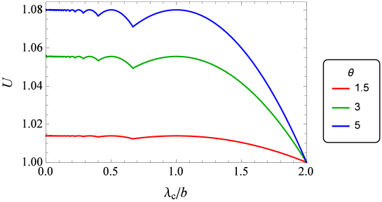
Figure 14: The flame speed versus $\lambda_{\text{c}}/b$ as given by the pole solutions of Eq. (27).

References

- (1) V. A. Mikhelson, On the normal burning speed of explosive gaseous mixtures, Ph.D. thesis, Moscow University (1890) [in Russian].
- (2) G. H. Markstein, Experimental and theoretical studies of flame front stability, J. Aeron. Sci. 18, 199 (1951).
- (3) G. H. Markstein, Nonsteady Flame Propagation (New York, Pergamon, 1964).
- (4) M. Matalon and B. J. Matkowsky, Flames as gasdynamic discontinuities, J. Fluid Mech. 124, 239 (1982).
- (5) P. Pelce and P. Clavin, Influences of hydrodynamics and diffusion upon the stability limits of laminar premixed flames, J. Fluid Mech. 124, 219 (1982).
- (6) P. Clavin, Dynamic behavior of premixed flame fronts in laminar and turbulent flows, Prog. Energy Combust. Sci. 11, 1 (1985).
- (7) G. Darrieus, unpublished work presented at La Technique Moderne and at Le Congrès de Mécanique Appliquée (1938 and 1945).
- (8) L. D. Landau, On the theory of slow combustion, Acta Physicochimica URSS 19, 77 (1944).
- (9) G. I. Sivashinsky, Nonlinear analysis of hydrodynamic instability in laminar flames, Acta Astronaut. 4, 1177 (1977).
- (10) G. I. Sivashinsky and P. Clavin, On the nonlinear theory of hydrodynamic instability in flames, J. Phys. (Paris) 48, 193 (1987).
- (11) K. A. Kazakov, Exact equation for curved stationary flames with arbitrary gas expansion, Phys. Rev. Lett. 94, 094501 (2005); On-shell description of stationary flames, Phys. Fluids 17, 032107 (2005).
- (12) H. El-Rabii, G. Joulin, and K. A. Kazakov, Nonperturbative approach to the nonlinear dynamics of two-dimensional premixed flames, Phys. Rev. Lett. 100, 174501 (2008); G. Joulin, H. El-Rabii, and K. A. Kazakov, On-shell description of unsteady flames, J. Fluid Mech. 608, 217 (2008).
- (13) H. El-Rabii, G. Joulin, and K. A. Kazakov, Premixed flame propagation in channels of varying width, SIAM J. Appl. Math. 70, 3287 (2010).
- (14) Though extension of the on-shell description to three dimensions is still unavailable, the reason to believe in its existence is the same as in two dimensions. The formally infinite speed of sound, implied by the flow incompressibility, means that any change in the flame structure is instantly “felt” by the entire flow, and vice versa. All information about the flow at any instant can thus be thought of as imprinted in the on-shell fields at the same instant. On the other hand, these fields define, together with the flow conditions at the tube walls, boundary conditions for the entire gas flow. Therefore, the space-time history of these fields up to a given instant determines their subsequent evolution, hence provides an on-shell description of the flame dynamics.
- (15) K. A. Kazakov, Analytical treatment of 2D steady flames anchored in high-velocity streams, Physica D 239, 600 (2010).
- (16) K. A. Kazakov, Analytical study in the mechanism of flame movement in horizontal tubes, Phys. Fluids 24, 022108 (2012); II. Flame acceleration in smooth open tubes, Phys. Fluids 25, 082107 (2013); Erratum: 26, 039902 (2014).
- (17) K. A. Kazakov, Mechanism of partial flame propagation and extinction in a strong gravitational field, Phys. Rev. Lett. 115, 264501 (2015).
- (18) K. A. Kazakov, Premixed flame propagation in vertical tubes, Phys. Fluids 28, 042103 (2016).
- (19) D. G. Anderson, Iterative procedures for nonlinear integral equations, JACM 12(4):547 (1965).
- (20) M. A. Olshanskii and E. E. Tyrtshnikov, Iterative methods for linear systems: theory and applications (SIAM, 2014).
- (21) S. A. Matveev et al., Anderson acceleration method of finding steady-state particle size distribution for a wide class of aggregation-fragmentation models, [in print] (2017).
- (22) W. D. Hayes, The vorticity jump across a gasdynamic discontinuity, J. Fluid Mech. 2, 595 (1957).
- (23) A. G. Class, B. J. Matkowsky, and A. Y. Klimenko, A unified model of flames as gasdynamic discontinuities, J. Fluid Mech. 491, 11 (2003).
- (24) T. Amemiya, Advanced econometrics, (Harvard University Press, USA, 1985).
- (25) K. A. Kazakov and O. G. Kharlanov, A numerical algorithm for nonlinear integro-differential equations modelling steady flames [in preparation].
- (26) D. Vaynblat and M. Matalon, Stability of pole solutions for planar propagating flames: I. Exact eigenvalues and eigenfunctions & II. Properties of eigenvalues and eigenfunctions with implication to flame stability, SIAM J. Applied Math. 60, 679, 703 (2000).
- (27) P. Clavin and J. C. Graña-Otero, Curved and stretched flames: the two Markstein numbers, J. Fluid Mech. 686, 187 (2011).
- (28) A. Levy, An optical study of flammability limits, Proc. Royal Soc. (London), Ser. A, Mathematical and Physical Sciences, 283, 134 (1965).
- (29) G. I. Barenblatt, Ya. B. Zeldovich, and A. G. Istratov, On diffusional thermal instability of laminar flame. Prikl. Mekh. Tekh. Fiz. 2, 21 (1962).
- (30) G. Searby and D. Rochwerger, A parametric acoustic instability in premixed flames, J. Fluid Mech. 231, 529 (1991).
- (31) Z. Olami, B. Galanti, O. Kupervasser, and I. Procaccia, Random noise and pole dynamics in unstable front propagation, Phys. Rev. E55, 2649 (1997).
- (32) B. Galanti, O. Kupervasser, Z. Olami, and I. Procaccia, Dynamics and wrinkling of radially propagating fronts inferred from scaling laws in channel geometries, Phys. Rev. Lett. 80, 2477 (1998).
- (33) C. Almarcha, B. Denet, and J. Quinard, Premixed flames propagating freely in tubes, Combust. Flame 162, 1225 (2015).
- (34) M. A. Liberman et al., Numerical studies of curved stationary flames in wide tubes, Combust. Theory Modelling 7, 653 (2003).
- (35) K. A. Kazakov and M. A. Liberman, Nonlinear equation for curved stationary flames, Phys. Fluids 14, 1166 (2002).
- (36) V. Sadovnichy, A. Tikhonravov, V. Voevodin, and V. Opanasenko, “Lomonosov”: Supercomputing at Moscow State University, in Contemporary High Performance Computing: From Petascale toward Exascale, Ed. by J. S. Vetter (CRC Press, USA, 2013), p. 283.
- (37) O. Thual, U. Frish, and M. Henon, Application of pole decomposition to an equation governing the dynamics of wrinkled flames, J. Phys. (France) 46, 1485 (1985).