Abstract

In this paper, we study large multi-server loss models under power-of-$d$ routing scheme when service time distributions are general with finite mean. Previous works have addressed the exponential service time case when the number of servers goes to infinity giving rise to a mean field model. The fixed point of limiting mean field equations (MFE) was shown to be insensitive to the service time distribution through simulation. Showing insensitivity to general service time distributions has remained an open problem. Obtaining the MFE in this case poses a challenge due to the resulting Markov description of the system being in positive orthant as opposed to a finite chain in the exponential case. In this paper, we first obtain the MFE and then show that the MFE has a unique fixed point that coincides with the fixed point in the exponential case thus establishing insensitivity. The approach is via a measure-valued Markov process representation and the martingale problem to establish the mean-field limit. The techniques can be applied to other queueing models.

Keywords: Erlang loss models, power-of-d, mean field, measure-valued processes, fixed-point, insensitivity.

AMS Classification Primary: 60K35Secondary 60F10;60J10;62F15

1 Introduction

We consider a multi-server loss system consisting of $N$ large number of parallel servers to which jobs arrive according to a Poisson process with rate $N\lambda$ and the service times are generally distributed with finite mean. Each server has the capacity to serve up to $C$ number of jobs simultaneously and there is no waiting room. A central job dispatcher routes an incoming job to one of the servers where the processing of the job begins immediately if the number of jobs that are already in progress is less than $C$ otherwise, the job gets blocked. These models appear in practice in cloud computing systems such as Microsoft’s Azure [22] and Amazon EC2 [2].

Due to a tremendous growth in Internet applications and the move to externalize storage and computing, cloud computing systems maintain a large number of parallel servers to provide service to incoming jobs. In these systems, jobs are virtual machines(VMs) that request resources such as processor power, I/O bandwidth, disk etc. from a server that is picked from a large set of servers. Whenever a job arrives, the central job dispatcher routes an incoming job request to one of the servers where the job will be processed immediately if the requested amount of resources are available otherwise it is blocked. The resources allocated to a job will be released once the service of a job ends. In order to provide good quality of service, the service provider in cloud computing systems uses the routing policy at the job dispatcher that balances loads on servers which results in minimum average blocking probability. In general, load balancing is an efficient method to optimally use the resources of a system which results in better system performance. In the large scale cloud computing systems that contain thousands of servers, the traditional optimal load balancing schemes such as the join-the-shortest-queue (JSQ) results in large computational cost and complexity due to the need to maintain the states of all servers. One way of overcoming this is by using randomized algorithms that are based on sampling a subset of servers and adopting a shortest-queue (SQ) policy amongst them. It has been shown that such algorithms are almost as good as JSQ.

The power-of-$d$ routing policy that routes incoming requests to the shortest of $d$ uniformly sampled servers was first introduced in [35] for multi-server server systems with FCFS service discipline for the case of $d=2$ and exponential service times. The analysis of a finite $N$ system under the power-of-$d$ routing policy is a difficult problem due to dependence amongst the servers introduced by the random sampling, however using mean-field techniques when $N\to\infty$ provide a tractable way of characterizing the stationary distributions that are accurate when the number $N$ is large. Indeed the analysis in [35] is based on this idea. The results were then extended for the case of $d>2$ in [23] where it was argued that the case $d=2$ provides most of the gains and whence the term ‘The power-of-2’ came to be used.

Loss models similar to the one considered in this paper were analyzed in [36, 26] under the assumption of exponential service times for the power-of-$d$ routing policy. They considered the more general heterogeneous case with different server capacities and jobs routed to servers with maximum vacancy among $d$ randomly chosen servers. It was shown that the power-of-$d$ routing scheme yields almost optimal blocking performance in that the average blocking is very close to the theoretical lower bound on the minimum average blocking achievable by any work conserving policy.

The complete analysis of queuing systems under the power-of-$d$ routing policy using mean-field techniques can be summarized as in the Figure 1. There are four steps in the complete analysis of the system. The first step is to establish the mean-field limit. In the exponential service time case, the system dynamics are first represented as a Markov process $\mathbf{x}^{N}(t)=(x^{N}_{l}(t),l\geq 0)$ where $x_{l}^{N}(t)$ denotes the fraction of servers with at least $l$ jobs, and then as $N\to\infty$, the process $(\mathbf{x}^{N}(t))_{t\geq 0}$ was shown to converge weakly to a system of ordinary differential equations that have unique solution called as the mean-field limit (MFE). The second step is to show the global stability of the mean-field limt $(\bm{x}(t,\mathbf{u}))_{t\geq 0}$ where $\mathbf{u}$ denotes the initial point of the mean-field i.e., $\bm{x}(0,\mathbf{u})=\bm{u}$. So far, in the literature, step two is shown only for the case when mean-field equations satisfy the quasi-monotonicity[35]. The quasi-monotonicity is described as follows. The quasi-monotonicity implies that if $\bm{u_{1}}\geq\bm{u_{2}}$ by element wise, then $\bm{x}(t,\bm{u_{1}})\geq\bm{x}(t,\bm{u_{2}})$ by element wise for every $t\geq 0$. Step two is very difficult to establish when mean-field equations do not satisfy the quasi-monotonicity property. The third step follows from ergodicity when system with finite $N$ servers is stable. The fourth step can be shown by combining step two, step three and Prohorov’s theorem [4]. The fourth step is crucial to use the fixed-point of the mean-field as an approximation to the steady-state distribution for server occupancies in a system with large $N$. Combining four steps, we have

$$\lim_{N\to\infty}\lim_{t\to\infty}\mathbf{x}^{N}(t)=\lim_{t\to\infty}\lim_{N\to\infty}\mathbf{x}^{N}(t).$$ (1.1)

Figure 1: Commutativity of limits

Further, for multi-server loss sytem with capacity $C$ for each server, if $\mathbf{P}^{(exp)}=(P_{n}^{(exp)},0\leq n\leq C)$ such that $P_{0}^{(exp)}=1$ and $P_{n}^{(exp)}\geq P_{n+1}^{(exp)}$, then for exponential service times case, it was shown in [36, 26] that the unique fixed-point of the mean-field is same as the unique fixed-point of the mapping $\mathbf{\theta}(\mathbf{P}^{exp})$ defined by

$$\mathbf{\theta}(\mathbf{P}^{(exp)})=\mathcal{S}(\Lambda(\mathbf{P}^{(exp)}),\mathbf{P}^{(exp)}),$$ (1.2)

where for $0\leq n\leq C$ with $P_{C+1}^{(exp)}=0$,

$$\Lambda(\mathbf{P}^{(exp)}):\,\,\,\lambda_{n}=\lambda\frac{((P_{n}^{exp})^{d}-(P_{n+1}^{(exp)})^{d})}{(P_{n}^{(exp)}-P_{n+1}^{(exp)})}$$ (1.3)

and

$$\mathcal{S}(\Lambda,\mathbf{P}^{(exp)}):\,\,\,\,\lambda_{n}(P_{n}^{(exp)}-P_{n+1}^{(exp)})=(n+1)(P_{n+1}^{(exp)}-P_{n+2}^{(exp)})\mu.$$ (1.4)

The exchange of limits as in equation (1.1), allows us to study the impact of the power-of-$d$ routing policy by characterizing the fixed-point of the mean-field. However, the exchange of limits in equation (1.1) was established under the assumption that the service times are exponential. In most realistic applications, the service time distributions are not exponential. For example, service times follow Log-normal distributions in call centers [7], and Gamma distributions in automatic teller machines (ATMs) [21] etc.

For general service times case, the Markovian modeling of the system requires us to track the age or residual service time of each job that is in progress in the system. Therefore the underlying space on which the Markov process is defined is uncountable. This makes establishing the mean-filed limit and then establishing the exchange of limits in equation (1.1) for general service times a challenging task.

It is well known that the stationary distributions of single loss systems even with prespecified state-dependent arrival rates are insensitive to the service time distribution, i.e., they only depend on the means of the service times [8]. Hence, it is important to investigate insensitivity of large multi-server loss systems with general service time distributions under the power-of-$d$ routing policy where the servers are coupled for finite $N$. Insensitivity was observed in the simulations in [36, 26] but there were no proofs provided. The first step is thus to establish the mean-field limit and analyze its equilibrium behavior.

1.1 Related Literature

Randomized routing schemes were first investigated in [3] using balls-and-bins models. The power-of-$d$ scheme was considered for FCFS queues with exponential service time distributions in [23, 35]. It was shown that in the limiting system, the probability that a queue has atleast $k$ jobs is equal to $\lambda^{\frac{d^{k}-1}{d-1}}$ for $d\geq 2$ while it is equal to $\lambda^{k}$ for the case of $d=1$. This shows that the steady-state tail probabilities decrease double-exponentially with queue lengths for $d\geq 2$ whereas it is exponential decay for $d=1$.

The significant improvement in system performance (in terms of buffer occupancy) for FCFS systems under the power-of-$d$ routing policy was also shown for processor sharing (PS) queues in [24, 25] when service times are exponentially distributed. In [5], randomized routing schemes for queueing systems with general service time distributions when service disciplines are FCFS, PS, and LIFO were studied. The steady-state results were characterized by assuming propagation of chaos (or asymptotic independence of servers) in the system. The propagation of chaos for FCFS systems is established in [6] for the case when service time distributions have decreasing hazard rate functions. In [5] the approach was to study the impact of the power-of-$d$ routing policy by characterizing the stationary distribution of the limiting system by considering step $3$ and step $4$ of Figure 1. The mean-filed limit and its fixed-point were not studied.

For general service times case [19] obtained the mean-field for symmetric closed queueing networks with FCFS service discipline that consist of $N$ queues and $M$ customers in which a customer that exits a queue joins a queue that is picked with probability $\frac{1}{N}$ from $N$ queues. The mean-field was established for the regime when $N\to\infty$, $M\to\infty$ such that $\frac{M}{N}\to\alpha$ using the convergence of infinitesimal generators of Markov processes that represent the system dynamics. However, the equilibrium behavior of the system is not studied. Recently, [1] considered a system of $N$ FCFS servers and jobs arrive according to a time-inhomogeneous Poisson process with rate $\lambda^{(N)}(\cdot)=a^{(N)}\lambda(\cdot)$ where $\lambda(\cdot)$ is a locally non-negative function with $\frac{a^{(N)}}{N}\to 1$ as $N\to\infty$. The mean-field limit is established for general service time distributions under the power-of-$d$ routing policy for all compact intervals of time. However, the steady-state results were not investigated.

Multi-server loss models under randomized routing schemes were first studied in [31, 32] when job lengths are exponentially distributed by using mean-field techniques. The mean-field equations were used to characterize the limiting system and the resulting tail distribution of server occupancies observed to decay rapidly even when there is a small number of routing choices for each arriving job. However, the existence and uniqueness of the fixed-point of the mean-field were not shown. In [36], the existence and uniqueness of the fixed-point of the mean-field for homogeneous loss model of [31] was addressed. The heterogeneous case was also treated in [36] under the asymptotic independence of servers ansatz. The propagation of chaos (or independence on path space) was studied earlier by [12, 13] in the context of alternate routing in circuit-switched networks.

The complete analysis for heterogeneous loss models under the power-of-$d$ routing scheme when service times are exponential is given in [26]. They showed the existence and uniqueness of the stationary point of the mean-field, as well as the global asymptotic stability of the mean-field. Further, the propagation of chaos was shown using intra-type exchangeability of random variables corresponding to server occupancies. The results were then extended to multi-class heterogeneous loss models in [27] where jobs belong to one of the several classes based on the amount of resources they use. All these works were based on the assumption that the job lengths are exponentially distributed. The study of large multi-server loss models with general service time distributions under power-of-$d$ routing and the proof of the insensitivity have not been addressed so far in the literature.

There is a close connection between the mean-field analysis and the fluid analysis of queues. The fluid limit analysis of complex queuing systems with general service time distributions was carried out by representing the system dynamics as a measure-valued process and then the fluid limit was established by showing the convergence of measure-valued processes using the theory developed by Dawson in [9]. In representing the system dynamics as a measure-valued process, either ages or residual service times of jobs can be used. Fluid limit analysis of different queuing systems using residual times can be found for heavily loaded processor sharing queues in [14], processor sharing queues with impatient customers in [15], M/GI/$\infty$ queue in [10], many-server queues with abandonment under FCFS service discipline in [37] etc. Fluid limit analysis using the ages of jobs to construct measure-valued processes can be found for many-server queues with FCFS service discipline in [20], many-server queues with reneging in [18] etc. In this paper, we use ages of jobs to construct the measure-valued Markov processes that represent the system dynamics and we establish the mean-field limit following the ideas in [10, 9].

1.2 Contributions and Organization of the paper

In this paper, we obtain and show that the mean-field for the power-of-d routing loss systems is well defined and we characterize the fixed-point or equilibrium of the mean field equation. In particular, we show that the fixed-point is unique and moreover coincides with the fixed point of the MFE in the exponential case. This establishes the insensitivity of the fixed point. In order to interpret the fixed point as the stationary distribution of the limiting model requires us to show that it is a globally asymptotically stable (GAS) equilibrium for the MFE. It appears very difficult to establish this and in the last section, we provide numerical evidence to show that it indeed seems to be true. We thus conjecture that this is true. In which case the results would then establish the insensitivity of the stationary distributions of the limiting loss system (system with $N\to\infty$) to service time distributions.

The rest of the paper is organized as follows: Section 2 describes the system model and the power-of-$d$ policy. In Section 3, we introduce the notation and construct various measure spaces required for the analysis. In Section 4, we provide a measure-valued representation for the state of the system. The mean-field equations are given in Section 5. The detailed proofs then follow in Sections 6 to 9. In Section 10, we then prove the main result on the uniqueness and characterization of the fixed point of the MFE thus showing that the fixed point is insensitive to the distribution and only depends on the mean service time. In Section 11, we state the generalization of the results we have obtained to systems with heterogeneous servers. The following Section 12 provides some evidence of the global asymptotic stability of the equilibrium of the MFE that indicates that Step 4 of the commutative diagram is indeed true. Finally, we close with some remarks and observations in Section 13.

2 System model and the routing policy

We consider a system consisting of $N$ large number of parallel servers that provide service to an incoming sequence of jobs arriving according to a Poisson process with rate $N\lambda$. The incoming jobs are routed to servers based on the predetermined routing policy implemented at the central job dispatcher. Further, each server is assumed to have capacity to serve up to $C$ number of jobs simultaneously and has no waiting room. At any time $t$, if a server is currently serving $i\leq C$ jobs, then we say that the server has occupancy $i$ and vacancy $C-i$ at time $t$. If an incoming job is routed to a server with occupancy $C$, then the job is blocked otherwise the processing of the job begins immediately.

Recently it was shown that the power-of-$d$ routing scheme achieves the performance (in terms of the average blocking) close to the optimal performance achievable by any work conserving strategy but with much less computational cost [36, 26]. We recall the power-of-$d$ routing policy which is the focus of this paper.

Definition 2.1

Power-of-d routing: An incoming job is routed to a server with minimum occupancy among $d$ randomly chosen servers. Ties among servers are broken by choosing a server uniformly at random. The randomly chosen $d$ servers are called as the potential destination servers and the server to which a job is routed is called as the destination server.

In this paper, we assume the service times are generally distributed with finite mean $\frac{1}{\mu}$ and the central job dispatcher routes an incoming job according to the power-of-$d$ policy. The service requirements of customers form an ${i.~{}i.~{}d.}$ sequence with distribution function $G(\cdot)$ on $[0,\infty)$ and the density function is $g(\cdot)$.

The hazard rate function of $G(\cdot)$ is denoted by $\beta(\cdot)$ satisfying $\beta(x)=\frac{g(x)}{\overline{G}(x)}=\frac{g(x)}{1-G(x)}$ for $x\in\mathcal{R}_{+}$. Note that the hazard rate function $\beta$ indicates the instantaneous rate at which the service of a job ends. More precisely, a job with age $y$ (where $y$ denotes the time since its arrival) at time $t$ exits the server in the interval $(t,t+dt]$ with probability $\beta(y)dt$.

Assumption 2.1

The hazard rate function $\beta$ satisfies

$$\beta\in\mathcal{C}_{b}(\mathcal{R}_{+}).$$ (2.5)

where $\mathcal{C}_{b}(\mathcal{R}_{+})$ denotes the space of continuous bounded functions on positive real line $\mathcal{R}_{+}$

3 Mathematical framework

3.1 Notation and terminology

We begin by introducing the notation which is used throughout the paper. Let $\mathcal{Z}$, $\mathcal{R}$ indicate the set of integers and real numbers, respectively. Further, let $\mathcal{Z}_{+}$, $\mathcal{R}_{+}$ indicate the set of nonnegative integers and nonnegative real numbers, respectively.

3.1.1 Function and measure spaces.

We next define the function spaces that are used in the analysis. For any given metric space $\mathcal{E}$, we define $\mathcal{K}_{b}(\mathcal{E}),\mathcal{C}_{b}(\mathcal{E}),\mathcal{C}_{s}(\mathcal{E})$ to denote the space of bounded measurable real valued functions, the space of bounded continuous real valued functions, and the space of continuous real valued functions with compact support, defined on $\mathcal{E}$, respectively. Further, let the space of once continuously differentiable real valued functions defined on $\mathcal{E}$ be denoted by $\mathcal{C}^{1}(\mathcal{E})$ and the subspace of functions in $\mathcal{C}^{1}(\mathcal{E})$ which have compact support is denoted by $\mathcal{C}^{1}_{s}(\mathcal{E})$. The space of bounded functions in $\mathcal{C}^{1}(\mathcal{E})$ whose first derivatives are also bounded is denoted by $\mathcal{C}^{1}_{b}(\mathcal{E})$. We then define, for any function $f\in\mathcal{K}_{b}(\mathcal{E})$, $h\in\mathcal{C}^{1}(\mathcal{E})$,

$$\|{f}\| =\sup_{x\in\mathcal{E}}\left|{f(x)}\right|$$ (3.6)

$$\|{h}\|_{1} =\|{h}\|+\|{h_{d}}\|$$ (3.7)

where $h_{d}$ is the first derivative of $h$. In particular, if $h:\mathcal{R}_{+}^{n}\mapsto\mathcal{R}$, then the $i^{\text{th}}$ directional derivative denoted by $h_{(d,i)}$ is defined as

$$h_{(d,i)}(x_{1},\ldots,x_{n})=\frac{\partial{h(x_{1},\ldots,x_{n})}}{\partial x_{i}}$$ (3.8)

and the first derivative $h_{d}=(h_{(d,i)},1\leq i\leq n)$ has the norm

$$\|{h_{d}}\| =\sup_{i}\sup_{(x_{1},\ldots,x_{n})\in\mathcal{R}_{+}^{n}}\left|{\frac{\partial{h(x_{1},\ldots,x_{n})}}{\partial x_{i}}}\right|$$ (3.9)

$$=\sup_{i}\|{h_{(d,i)}}\|.$$ (3.10)

The space $\mathcal{C}_{b}(\mathcal{E})$ is equipped with the uniform topology, ${i.e.}$, we say a sequence of functions $(f_{n}\in\mathcal{C}_{b}(\mathcal{E}),n\geq 1)$ converges to a function $f\in\mathcal{C}_{b}(\mathcal{E})$ if $\|{f_{n}-f}\|\to 0$ as $n\to\infty$. On the other hand, the space $\mathcal{C}^{1}(\mathcal{E})$ is equipped with the topology induced by the norm $\|{\cdot}\|_{1}$. For a function $f$ defined on $\mathcal{R}_{+}^{n}$, we define a function $f^{\prime}$ such that

$$f^{\prime}(x_{1},\ldots,x_{n})=\sum_{i=1}^{n}\frac{\partial f(x_{1},\ldots,x_{n})}{\partial x_{i}}.$$ (3.11)

For a given metric space $\mathcal{E}$, let the Borel $\sigma$-algebra be denoted by $\mathcal{B}(\mathcal{E})$. The space of finite non-negative measures on $\mathcal{E}$ is denoted by $\mathcal{M}_{F}(\mathcal{E})$. The measure value with respect to a measure $\nu\in\mathcal{M}_{F}(\mathcal{E})$ for a Borel set $B\in\mathcal{B}(\mathcal{E})$ is denoted by $\nu(B)$ and at a single element $y\in\mathcal{E}$ is denoted by $\nu(\{y\})$. The space of probability measures is denoted by $\mathcal{M}_{1}(\mathcal{E})$. Also, we define $\mathcal{M}_{1}^{N}(\mathcal{E})$ to denote the space of measures in $\mathcal{M}_{1}(\mathcal{E})$ that satisfy

$$\mathcal{M}_{1}^{N}(\mathcal{E})=\{\nu\in\mathcal{M}_{1}(\mathcal{E}):N\,\nu{(B)}\in\mathcal{Z}_{+},\,\forall B\in\mathcal{B}(\mathcal{E})\}.$$ (3.12)

Therefore $\mathcal{M}_{1}^{N}(\mathcal{E})$ is the set of all probability measures $\nu$ that have rational valued measure at every $B\in\mathcal{B}(\mathcal{E})$ with the denominator equal to $N$. The set of real valued continuous functions defined on $\mathcal{M}_{F}(\mathcal{E})$ is denoted by $\mathcal{C}(\mathcal{M}_{F}(\mathcal{E}))$. For any $\phi\in\mathcal{K}_{b}(\mathcal{E})$, $\nu\in\mathcal{M}_{F}(\mathcal{E})$, we define

$$\langle\nu,\phi\rangle=\int_{y\in\mathcal{E}}\phi(y)\nu(dy).$$ (3.13)

The space of measures $\mathcal{M}_{F}(\mathcal{E})$ is equipped with the weak topology according to which a sequence of measures $\nu_{n}\in\mathcal{M}_{F}(\mathcal{E})$ converge weakly to a measure $\nu\in\mathcal{M}_{F}(\mathcal{E})$ (denoted by $\nu_{n}\Rightarrow\nu$) if and only if

$$\langle\nu_{n},\phi\rangle\to\langle\nu,\phi\rangle$$ (3.14)

for every $\phi\in\mathcal{C}_{b}(\mathcal{E})$ as $n\to\infty$. Note that the space of measures $\mathcal{M}_{F}(\mathcal{E})$ endowed with the weak topology is a Polish space when $\mathcal{E}$ is a Polish space. The Dirac measure with unit mass at $x\in\mathcal{E}$ is denoted by $\delta_{x}$.

To model the dynamics of an Erlang loss system with capacity $C$ for each server as Markov process, we define the state of each server as $(n,a_{1},a_{2},\ldots,a_{n})$ where $n$ denotes the number of jobs that are in progress at the server and $a_{i}$ denotes the age of the $i^{\text{th}}$ job in progress. Recall the age of an active job is the time elapsed since its arrival. Therefore we define a metric space $\mathcal{U}$ such that it contains all the possible server states as elements, namely,

$$\mathcal{U}=\cup_{n=0}^{C}\mathcal{U}_{n}$$ (3.15)

where $\mathcal{U}_{0}=\{0\}$ and an element in $\mathcal{U}_{n}$ for $n\geq 1$ is of the form $(n,a_{1},\ldots,a_{n})$ where $1\leq n\leq C$ and $a_{i}\in\mathcal{R}_{+}$. We denote an element of the form $(n,u_{1},\ldots,u_{n})\in\mathcal{U}_{n}$ by $\underline{u}$. Without loss of generality, we also write $\underline{u}\in\mathcal{U}_{0}$ to mean that $\underline{u}=0$. Further, for all $B\in\mathcal{B}(\mathcal{U})$, $I_{\left\{{B}\right\}}$ denotes the indicator function of $B$, ${i.e.}$,

$$I_{\left\{{B}\right\}}(\underline{u})=\begin{cases}1&\text{if }\underline{u}\in B\\ 0&\text{otherwise}.\end{cases}$$ (3.16)

We define a function $\bm{1}$ that satisfies

$$\bm{1}(\underline{u})=1$$ (3.17)

for all $\underline{u}\in\mathcal{U}.$ The measure $\nu$ restricted to $\mathcal{U}_{0}$ is a Dirac measure at $\{0\}$. We say that the measure $\nu$ is continuous at $\underline{x}\in\mathcal{U}_{n}$ for $n\geq 1$ if and only if $\nu(\{\underline{x}\})=0$. For any Borel measurable function $f$ that is defined on $\mathcal{U}$ which is integrable with respect to $\nu\in\mathcal{M}_{F}(\mathcal{U})$, we define

$$\langle\nu,f\rangle =\int_{\underline{y}\in\mathcal{U}}f(\underline{y})\nu(d\underline{y})$$

$$=f(0)\nu(\{0\})+\sum_{n=1}^{C}\int_{\underline{z}\in\mathcal{U}_{n}}f(\underline{z})\nu(d\underline{z}).$$ (3.18)

For $\underline{y}=(n,y_{1},\ldots,y_{n}),\underline{z}=(m,z_{1},\ldots,z_{m})\in\mathcal{U}$, we define the metric $d_{\mathcal{U}}(\underline{y},\underline{z})$ as

$$d_{\mathcal{U}}(\underline{y},\underline{z})=\begin{cases}\sum_{i=1}^{n}\left|{y_{i}-z_{i}}\right|&\text{if }n=m\\ \infty&\text{otherwise}.\end{cases}$$ (3.19)

For any function $f:\mathcal{U}\to\mathcal{R}$, we define a function $f^{(i)}$ for $0\leq i\leq C$ referred to as the $i^{\text{th}}$ component of the function $f$ as follows:

$$f^{(0)}:\mathcal{U}_{0}\mapsto\mathcal{R}$$ (3.20)

such that

$$f^{(0)}(0)=f(0)$$ (3.21)

and

$$f^{(i)}:\mathcal{R}_{+}^{i}\mapsto\mathcal{R}$$ (3.22)

such that

$$f^{(i)}(x_{1},\ldots,x_{i})=f(i,x_{1},\ldots,x_{i}).$$ (3.23)

Similarly, for any measure $\nu\in\mathcal{M}_{F}(\mathcal{U})$, we define $i^{\text{th}}$ component of measure $\nu$ by $\nu^{(i)}$ such that

$$\nu^{(0)}=\nu{(\{0\})}\delta_{(0)}$$ (3.24)

and for $i\geq 1$,

$$\nu^{(i)}(\{(x_{1},\ldots,x_{i})\})=\nu{(\{(i,x_{1},\ldots,x_{i})\})}.$$ (3.25)

Therefore $\nu^{(n)}$ is a Borel measure defined on $(\mathcal{R}_{+}^{n},\mathcal{B}(\mathcal{R}_{+}^{n}))$. Therefore, for any Borel measurable function $f$ that is defined on $\mathcal{U}$ which is integrable with respect to $\nu\in\mathcal{M}_{F}(\mathcal{U})$, we can write

$$\langle\nu,f\rangle =\int_{\underline{y}\in\mathcal{U}}f(\underline{y})\nu(d\underline{y})$$

$$=f^{(0)}(0)\nu^{(0)}{(\{0\})}+\sum_{i=1}^{C}\int_{x_{1}\in\mathcal{R}_{+}}\cdots\int_{x_{i}\in\mathcal{R}_{+}}f^{(i)}(x_{1},\ldots,x_{i})\,d\nu^{(i)}(x_{1},\ldots,x_{i})$$ (3.26)

We say $f$ is differentiable if each component $f^{(i)}$, $i\geq 1$ is differentiable. For any $f:\mathcal{U}\mapsto\mathcal{R}$, we denote the first derivative by $f_{d}$ whose $i^{\text{th}}$ ($i\geq 1$) component is denoted by $f^{(i)}_{d}=(f_{(d,j)}^{(i)},1\leq j\leq i)$ where $f_{(d,j)}^{(i)},1\leq j\leq i)$ denotes the $j^{\text{th}}$ directional derivative of $f^{(i)}$ and we consider $f_{(d,0)}^{(0)}=0$ to be the first derivative of $f^{(0)}$. Note that from the definition of first derivative of a function, $f=I_{\left\{{\mathcal{U}_{n}}\right\}}$, $n\geq 0$ is differentiable as each $f^{(i)}$, $i\geq 1$ is differentiable.

We define a function $\mathcal{I}:\mathcal{U}\mapsto\mathcal{R}$ as follows

$$\mathcal{I}(n,x_{1},\ldots,x_{n})=(x_{1}+\ldots+x_{n})$$ (3.27)

for $n\geq 1$ and $\mathcal{I}(0)=0.$ Hence, we have

$$\langle\nu,\mathcal{I}\rangle=\sum_{n=1}^{C}\int_{x_{1}}\cdots\int_{x_{n}}(x_{1}+\cdots+x_{n})\,d\nu(n,x_{1},\ldots,x_{n}).$$ (3.28)

For any $\underline{u}\in\mathcal{U}_{n}$, $n\geq 1$ and for $y>0$, we define

$$\tau_{y}^{+}(n,u_{1},\ldots,u_{n})=(n,u_{1}+y,u_{2}+y,\ldots,u_{n}+y)$$ (3.29)

and

$$\tau_{y}^{+}(0)=(0).$$ (3.30)

For any $y>0,f\in\mathcal{K}_{b}(\mathcal{U})$, mapping $\tau_{y}:\mathcal{K}_{b}(\mathcal{U})\to\mathcal{K}_{b}(\mathcal{U})$ denotes,

$$\begin{split}\tau_{y}f(\underline{u})&=f(\tau_{y}^{+}\underline{u}).\end{split}$$ (3.31)

For $y>0$, we define a shifted measure $\tau_{y}\nu\in\mathcal{M}_{F}(\mathcal{U})$ such that for any Borel set $B\in\mathcal{B}(\mathcal{U})$,

$$\tau_{y}\nu{(B)}=\nu(\tau_{y}^{+}(B)).$$ (3.32)

For $\nu\in\mathcal{M}_{F}(\mathcal{U})$, the measure $\tau_{y}\nu\in\mathcal{M}_{F}(\mathcal{U})$ satisfies

$$\langle\tau_{y}\nu,f\rangle=\langle\nu,\tau_{y}f\rangle$$ (3.33)

for all $f\in\mathcal{K}_{b}(\mathcal{U})$. Existence of the unique measure $\tau_{y}\nu$ satisfying equation (3.33) follows from Riesz-Markov-Kakutani theorem [33, 29].

3.1.2 Measure valued stochastic processes.

For given Polish space $\mathcal{H}$, we denote the càdlàg functions that take values in $\mathcal{H}$ defined on $[0,T]$, $[0,\infty)$ by $\mathcal{D}_{\mathcal{H}}([0,T]),\mathcal{D}_{\mathcal{H}}([0,\infty))$, respectively. Similarly, we denote the continuous functions that take values in $\mathcal{H}$ defined on $[0,T]$, $[0,\infty)$ by $\mathcal{C}_{\mathcal{H}}([0,T]),\mathcal{C}_{\mathcal{H}}([0,\infty))$, respectively. The spaces $\mathcal{D}_{\mathcal{H}}([0,T])$,$\mathcal{D}_{\mathcal{H}}([0,\infty))$ are equipped with the Skorokhod $J_{1}$-topology and hence they are Polish spaces. The covariation between of two local martingales $(M^{1}_{t})_{t\geq 0}$ and $(M^{2}_{t})_{t\geq 0}$ in $\mathcal{D}_{\mathcal{R}}([0,T])$ is denoted by $(<M^{1},M^{2}>_{t})_{t\geq 0}$ and the (quadratic) variation by $(<M^{1}>_{t})_{t\geq 0}=(<M^{1},M^{1}>_{t})_{t\geq 0}$.

In our analysis, we study $\mathcal{H}-$valued stochastic process where $\mathcal{H}=\mathcal{M}_{F}(\mathcal{U})$. The considered stochastic processes are random elements defined on $(\Omega,\mathbb{F},\mathcal{P})$ with sample paths in $\mathcal{D}_{\mathcal{H}}([0,\infty))$ and are equipped with the Borel $\sigma-$algebra generated by the open sets under the Skorokhod $J_{1}-$ topology [4]. We say a sequence $\{X_{n}\}$ of $\mathcal{H}$-valued càdlàg processes defined on $(\Omega_{n},\mathbb{F}_{n},\mathcal{P}_{n})$ converge in distribution to a $\mathcal{H}$-valued càdlàg process $X$ defined on $(\Omega,\mathbb{F},\mathcal{P})$ if, for every bounded, continuous, real valued functional $F:\mathcal{D}_{\mathcal{H}}:[0,\infty)\to\mathcal{R}$, we have

$$\lim_{n\to\infty}\mathbb{E}_{n}(F(X_{n}))=\mathbb{E}(F(X))$$ (3.34)

where the expectation operators $\mathbb{E}_{n},\mathbb{E}$ are defined with respect to $\mathcal{P}_{n},\mathcal{P}$, respectively. We denote the convergence of $\{X_{n}\}$ in distribution to $X$ by $X_{n}\Rightarrow X$.

4 State descriptor and system dynamics

For finite $N$, the evolution of the system is obtained by considering the state of each server to be $(n,a_{1},\ldots,a_{n})\in\mathcal{U}$ where $n$ denotes the number of jobs that are in progress and $a_{i}$ denotes the age of the $i^{\text{th}}$ job. Each server with state say $(n,a_{1},\ldots,a_{n})$ can be viewed as an atom with the given state. Therefore the system evolution can be considered as the evolution of the system with $N$ atoms where the interactions between atoms takes place while implementing the power-of-$d$ policy when there is an arrival into the system. The age of a job that is in service at a server increases linearly with time until its service expires.

We next describe the possible state for a server at time $t+h$ ($h>0$) given that it has state $(n,a_{1},\ldots,a_{n})$ at time $t$ by assuming that atmost one event can occur in the interval $(t,t+h]$. In the interval $(t,t+h]$, if there is no arrival into the given server and there is no departure from the given server, then the server state will be equal to $\tau_{h}^{+}(n,a_{1},\ldots,a_{n})$ at time $t+h$. Further, if $i^{\text{th}}$ job expires in the interval $(t,t+h]$, then the server state will be equal to $(n-1,a_{1}+h,\ldots,a_{i-1}+h,a_{i+1}+h,\ldots,a_{n}+h)$ at time $t+h$. Considering arrivals, suppose there is an arrival into the server at time $t+h^{\prime}$($0<h^{\prime}\leq h$), then the arriving job chooses its position uniformly at random out of $n+1$ possible positions and suppose it chooses $j^{\text{th}}$ position, then the server state will be equal to $(n+1,a_{1}+h,\ldots,a_{j-1}+h,h-h^{\prime},a_{j}+h,\ldots,a_{n}+h)$ at time $t+h$.

Since servers are identical, to model the system evolution by a Markov process, we will show that it is enough to just keep track of the number of servers that lie in each state $\underline{u}\in\mathcal{U}$. Precisely, the state descriptor of the system is denoted by

$$\eta_{t}^{N}=\sum_{i=1}^{N}\delta_{s_{t}(i)},$$ (4.35)

where $s_{t}(i)\in\mathcal{U}$ denotes the state of server $i$ at time $t$. Note that the mass of $\eta_{t}^{N}$ at a state $\underline{u}\in\mathcal{U}$ is equal to the number of servers with state $\underline{u}$ at time $t$. Therefore, the mass at state $(n,y_{1},\ldots,y_{n})$ is given by

$$\eta_{t}^{N}(\{(n,y_{1},\ldots,y_{n})\})=\langle\eta_{t}^{N},I_{\left\{{(n,y_{1},\ldots,y_{n})}\right\}}\rangle.$$ (4.36)

Similarly, the number of servers having $n$ jobs in progress at time $t$ is given by

$$\eta_{t}^{N}(\mathcal{U}_{n})=\langle\eta_{t}^{N},I_{\left\{{\mathcal{U}_{n}}\right\}}\rangle.$$ (4.37)

We next describe the dynamics of $(\eta_{t}^{N})_{t\geq 0}$ over time $t$. Suppose at time $t$, the measure $\eta_{t}^{N}$ is given by

$$\eta_{t}^{N}=\sum_{i=1}^{N}\delta_{(n_{i},a_{i1},\ldots,a_{in_{i}})}.$$ (4.38)

If there is no arrival into the system or departure from the system in the interval $(t,t+h]$, then the mass with respect to ($w.r.t.$) the measure $\eta_{t}^{N}$ at any state $(m,y_{1},\ldots,y_{m})\in\mathcal{U}$ will be equal to the mass at $(m,y_{1}+h,\ldots,y_{m}+h)$ $w.r.t.$ the measure $\eta_{t+h}^{N}$. If there is a departure in the interval $(t,t+h]$ from a server with state $(m,y_{1},\ldots,y_{m})$ at time $t$ and the job at position $j$ departs, then we have

$$\eta_{t+h}^{N}(\{(m,y_{1}+h,\ldots,y_{m}+h)\})=\eta_{t}^{N}(\{(m,y_{1},\ldots,y_{m})\})-1,$$ (4.39)

$$\eta_{t+h}^{N}(\{(m-1,y_{1}+h,\ldots,y_{j-1}+h,y_{j+1}+h,\ldots,y_{m}+h)\})\\ =\eta_{t}^{N}(\{(m-1,y_{1},\ldots,y_{j-1},y_{j+1},\ldots,y_{m})\})+1$$ (4.40)

and for all other states of the form $\underline{u}=(r,l_{1},\ldots,l_{r})\in\mathcal{U}$ such that $\underline{u}\neq(m,y_{1},\ldots,y_{m})$ and $\underline{u}\neq(m-1,y_{1},\ldots,y_{j-1},y_{j+1},\ldots,y_{m})$, we have

$$\eta_{t+h}^{N}(\{(r,l_{1}+h,\ldots,l_{r}+h)\})=\eta_{t}^{N}(\{(r,l_{1},\ldots,l_{r})\}).$$ (4.41)

On the other hand, when there is an arrival into the system at time $t+h^{\prime}$ ($0<h^{\prime}\leq h$) and suppose the arriving job occupies position $j$ at a server that had state $(m,y_{1},\ldots,y_{m})$ at time $t$, then we have

$$\eta_{t+h}^{N}(\{(m,y_{1}+h,\ldots,y_{m}+h)\})=\eta_{t}^{N}(\{(m,y_{1},\ldots,y_{m})\})-1,$$ (4.42)

$$\eta_{t+h}^{N}(\{(m+1,y_{1}+h,\ldots,y_{j-1}+h,h-h^{\prime},y_{j}+h,y_{j+1}+h,\ldots,y_{m}+h)\})=1$$ (4.43)

and for all other states of the form $\underline{u}=(r,l_{1},\ldots,l_{r})\in\mathcal{U}$ such that $\underline{u}\neq(m,y_{1},\ldots,y_{m})$, we have,

$$\eta_{t+h}^{N}(\{(r,l_{1}+h,\ldots,l_{r}+h)\})=\eta_{t}^{N}(\{(r,l_{1},\ldots,l_{r})\}).$$ (4.44)

Further, it is easy to see that $\eta_{t}^{N}\in\mathcal{M}_{F}(\mathcal{U})$, $(\eta_{t}^{N})_{t\geq 0}\in D_{\mathcal{M}_{F}(\mathcal{U})}([0,\infty)$ and $\eta_{t}^{N}(\mathcal{U})=N$ for all $t\geq 0$.

5 Mean-field model

In this section we introduce the mean-field model for the system and state our main results. In this paper, we study a sequence of systems indexed by $N$ such that a system with index $N$ has $N$ servers in which jobs arrive according to a Poisson process with rate $N\lambda$ and all other system parameters are identical for all $N$. For given $N$, the process $(\eta_{t}^{N})_{t\geq 0}$ defined in equation (4.35) describes the system dynamics of a system with index $N$ such that $\eta_{t}^{N}(\{\underline{u}\})$ denotes the number of servers lying in state $\underline{u}$ at time $t$. Our aim is to characterize the limit of the normalized process $(\overline{\eta}_{t}^{N})_{t\geq 0}$ defined as follows

$$\overline{\eta}_{t}^{N}=\frac{\eta_{t}^{N}}{N}.$$ (5.45)

For given system parameters $\lambda,C,d$ and the probability density function $g(\cdot)$ of the service time distributions, for analysis purpose, we first define the mean-field model $(\overline{\eta}_{t},t\geq 0)$ for the system in Definition 5.1 and we then show that there exists unique mean-field model solution. The mean-field model that we define acts as a fluid limit of the measure-valued state descriptors $(\eta_{t}^{N},t\geq 0)$ under law of large numbers scaling. Precisely, we show that every limit point of the sequence of the processes $(\overline{\eta}_{t}^{N})_{t\geq 0}$ has almost surely continuous sample paths that coincide with the unique mean-field model solution.

Mean-field model:
The dynamics of the mean-field model $(\overline{\eta}_{t},t\geq 0)$ are described by using the set of evolution equations for the real valued process $\langle\overline{\eta}_{t},f\rangle_{t\geq 0}$, for all $f\in\mathcal{C}_{b}^{1}(\mathcal{U})$, referred to as the mean-field model equations.

Definition 5.1

Mean-field model solution: A mean-field model solution for the given system parameters $(\lambda,C,d,g(\cdot))$ is a function $\overline{\eta}:[0,\infty)\mapsto\mathcal{M}_{1}(\mathcal{U})$ that satisfy

1. The mapping $t\mapsto\overline{\eta}_{t}$ is a continuous mapping. This is equivalent to the continuity of the mapping $t\mapsto\langle\overline{\eta}_{t},\phi\rangle$ for all $\phi\in\mathcal{C}_{b}(\mathcal{U})$ since $\mathcal{C}_{b}(\mathcal{U})$ is a separating class[11, p. 111].

2. For $\phi\in\mathcal{C}_{b}^{1}(\mathcal{U})$, the process $(\overline{\eta}_{t},t\geq 0)$ satisfies

   $$\langle\overline{\eta}_{t},\phi\rangle=\langle\overline{\eta}_{0},\phi\rangle+\int_{s=0}^{t}\langle\overline{\eta}_{s},\phi^{\prime}\rangle\,ds\\ -\int_{s=0}^{t}\Bigg{(}\sum_{n=1}^{C}\sum_{j=1}^{n}\int_{x_{1}}\cdots\int_{x_{n}}\beta(x_{j})\\ \times\left(\phi(n-1,x_{1},\ldots,x_{j-1},x_{j+1},\ldots,x_{n})-\phi(n,x_{1},\ldots,x_{n})\right)\,d\overline{\eta}_{s}(n,x_{1},\ldots,x_{n})\\ +\lambda\bigg{[}\left(\overline{\eta}_{s}(\{0\})\frac{(\overline{R}_{0}(\overline{\eta}_{s})^{d}-\overline{R}_{1}(\overline{\eta}_{s})^{d})}{(\overline{R}_{0}(\overline{\eta}_{s})-\overline{R}_{1}(\overline{\eta}_{s}))}\left(\phi(1,0)-\phi(0)\right)\right)+\sum_{n=1}^{C-1}\sum_{j=1}^{n+1}\int_{x_{1}}\cdots\int_{x_{n}}\frac{1}{(n+1)}\\ \times\frac{(\overline{R}_{n}(\overline{\eta}_{s})^{d}-\overline{R}_{n+1}(\overline{\eta}_{s})^{d})}{(\overline{R}_{n}(\overline{\eta}_{s})-\overline{R}_{n+1}(\overline{\eta}_{s}))}(\phi(n+1,x_{1},\ldots,x_{j-1},0,x_{j},\ldots,x_{n})-\phi(n,x_{1},\ldots,x_{n}))\\ \times\,d\overline{\eta}_{s}(n,x_{1},\ldots,x_{n})\bigg{]}\Bigg{)}ds,$$ (5.46)

where $\overline{R}_{j}(\overline{\eta}_{s})=\sum_{n=j}^{C}\overline{\eta}_{s}(\mathcal{U}_{n})$.

The equation (5.46) defined for each $\phi\in\mathcal{C}_{b}^{1}(\mathcal{U})$ is referred to as the mean-field model equation.

The mean-field model equation (5.46) is defined for class of functions $\phi\in\mathcal{C}_{b}^{1}(\mathcal{U})$, however, since one would be more interested to understand the fluid limit approximation of the process $(\langle\overline{\eta}_{t}^{N},I_{\left\{{B}\right\}}\rangle,t\geq 0)$ for a Borel set $B\in\mathcal{B}(\mathcal{U})$, it would be more useful to obtain the evolution equations for the real valued process of type $(\langle\overline{\eta}_{t},I_{\left\{{B}\right\}}\rangle,t\geq 0)$. In this direction, we first obtain the evolution equations for the real valued process $(\langle\overline{\eta}_{t},\psi\rangle,t\geq 0)$ where $\psi\in\mathcal{C}_{b}(\mathcal{U})$. We later obtain the evolution equations for the process $(\langle\overline{\eta}_{t},\psi\rangle,t\geq 0)$ for class of functions $\psi$ that also include functions of type $I_{\left\{{B}\right\}}$ for some $B\in\mathcal{B}(\mathcal{U})$.

Lemma 5.1

A process $(\nu_{t}\in\mathcal{M}_{1}(\mathcal{U}),t\geq 0)$ which is a continuous function of $t$ satisfies the mean-field model equation (5.46) if and only if it satisfies the equation, for all $\phi\in\mathcal{C}_{b}(\mathcal{U})$,

$$\langle\nu_{t},\phi\rangle=\langle\nu_{0},\tau_{t}\phi\rangle+\int_{r=0}^{t}\Bigg{(}\sum_{n=1}^{C}\sum_{j=1}^{n}\int_{x_{1}}\cdots\int_{x_{n}}\beta(x_{j})\\ \times\left(\tau_{t-r}\phi(n-1,x_{1},\ldots,x_{j-1},x_{j+1},\ldots,x_{n})-\tau_{t-r}\phi(n,x_{1},\ldots,x_{n})\right)\,d\nu_{r}(n,x_{1},\ldots,x_{n})\\ +\lambda\bigg{[}\left(\nu_{r}(\{0\})\frac{(\overline{R}_{0}(\nu_{r})^{d}-\overline{R}_{1}(\nu_{r})^{d})}{(\overline{R}_{0}(\nu_{r})-\overline{R}_{1}(\nu_{r}))}\left(\tau_{t-r}\phi(1,0)-\tau_{t-r}\phi(0)\right)\right)+\sum_{n=1}^{C-1}\sum_{j=1}^{n+1}\int_{x_{1}}\cdots\int_{x_{n}}\frac{1}{(n+1)}\\ \times\frac{(\overline{R}_{n}(\nu_{r})^{d}-\overline{R}_{n+1}(\nu_{r})^{d})}{(\overline{R}_{n}(\nu_{r})-\overline{R}_{n+1}(\nu_{r}))}(\tau_{t-r}\phi(n+1,x_{1},\ldots,x_{j-1},0,x_{j},\ldots,x_{n})-\tau_{t-r}\phi(n,x_{1},\ldots,x_{n})),\\ \times\,d\nu_{r}(n,x_{1},\ldots,x_{n})\bigg{]}\Bigg{)}\,dr,$$ (5.47)

where $\overline{R}_{j}(\nu_{s})=\sum_{n=j}^{C}\nu_{s}(\mathcal{U}_{n})$.

Using equation (5.47), we next state a result that shows that starting with an initial measure $\nu_{0}$, for $t\geq 0$, there exists unique measure $\nu_{t}\in\mathcal{M}_{1}(\mathcal{U})$ satisfying equation (5.46).

Since for $\nu\in\mathcal{M}_{F}(\mathcal{U})$, $\langle\nu,\phi\rangle$ is a continuous linear operator on the space of functions $\phi\in\mathcal{C}_{b}(\mathcal{U})$, we define

$$\|{\nu}\|=\sup_{\phi\in\mathcal{C}_{b}(\mathcal{U})}\frac{\left|{\langle\nu,\phi\rangle}\right|}{\|{\phi}\|}.$$ (5.48)

Theorem 5.1

There exists unique solution in $\mathcal{C}_{\mathcal{M}_{1}(\mathcal{U})}([0,\infty))$ satisfying the mean-field model equations. In particular, if $(\nu_{t}^{1},t\geq 0)$ and $(\nu_{t}^{2},t\geq 0)$ are two mean-field model solutions starting at initial measures $\nu_{0}^{1}\in\mathcal{M}_{1}(\mathcal{U})$, $\nu_{0}^{2}\in\mathcal{M}_{1}{\mathcal{(U)}}$, respectively, then

$$\|{\nu_{t}^{1}-\nu_{t}^{2}}\|\leq\|{\nu_{0}^{1}-\nu_{0}^{2}}\|\,e^{(2C\|{\beta}\|+8d^{2}\lambda)t}.$$ (5.49)

Mean-field limit:
We next state the results on convergence of sequence of processes $(\overline{\eta}_{t}^{N},t\geq 0)$. For this, we first make the following assumption:

Assumption 5.1

The sequence of initial measures of the normalized measure-valued processes $(\overline{\eta}_{t}^{N},t\geq 0)$ satisfy

$$\overline{\eta}_{0}^{N}\Rightarrow\bm{\Theta}$$ (5.50)

where $\Theta$ is a random measure taking values in $\mathcal{M}_{1}(\mathcal{U})$.

Theorem 5.2

If the sequence of processes $(\overline{\eta}^{N}_{t},t\geq 0)$ satisfy the assumption 5.1, then we have $\overline{\eta}^{N}\Rightarrow\overline{\eta}$. The process $(\overline{\eta}_{t},t\geq 0)$ is referred to as the mean-field limit that has sample paths almost surely coinciding with the unique mean-field model solution.

Remark 5.1

For any closed or open subset $B\in\mathcal{U}$, once we have $\overline{\eta}^{N}\Rightarrow\overline{\eta}$, if $\overline{\eta}_{t}$ is absolutely continuous $w.r.t.$ Lebesgue measure for every $t\geq 0$, then continuous mapping theorem implies that $\langle\overline{\eta}^{N},I_{\left\{{B}\right\}}\rangle\Rightarrow\langle\overline{\eta},I_{\left\{{B}\right\}}\rangle$. This shows that for large $N$, the fluid limit approximation of $\langle\overline{\eta}^{N},I_{\left\{{B}\right\}}\rangle$ is given by $\langle\overline{\eta},I_{\left\{{B}\right\}}\rangle$.

Insensitivity:
Before stating the results on the insensitivity of the fixed-point of the mean-field, we first recall the dynamics of probabilities of server occupancies of a single server Erlang loss system where jobs arrive according to a Poisson process with pre-specified state-dependent arrival rates. We observe an analogy between the mean-field equations of the considered multi-server Erlang loss system under power-of-$d$ routing policy and the single server system dynamics. We use this in proving the uniqueness of the fixed-point of the mean-field.

Consider a single server system with capacity $C$ where jobs arrive according to a Poisson process at rate $\alpha_{n}$ when there are $n$ jobs in service in the system. The service times are generally distributed as considered in the system model. It can be verified that the Kolmogorov equations are given by, for $\phi\in\mathcal{C}_{b}^{1}(\mathcal{U})$, let $\nu_{t}^{(single)}$ denotes the probability measure for server occupancies at time $t$, then

$$\langle\nu_{t}^{(single)},\phi\rangle=\langle\nu_{0}^{(single)},\phi\rangle+\int_{s=0}^{t}\langle\nu^{(single)}_{s},\phi^{\prime}\rangle\,ds\\ -\int_{s=0}^{t}\Bigg{(}\sum_{n=1}^{C}\sum_{j=1}^{n}\int_{x_{1}}\cdots\int_{x_{n}}\beta(x_{j})\\ \times\left(\phi(n-1,x_{1},\ldots,x_{j-1},x_{j+1},\ldots,x_{n})-\phi(n,x_{1},\ldots,x_{n})\right)\,d\nu^{(single)}_{s}(n,x_{1},\ldots,x_{n})\\ +\bigg{[}\left(\alpha_{0}\nu^{(single)}_{s}(\{0\})\left(\phi(1,0)-\phi(0)\right)\right)+\sum_{n=1}^{C-1}\sum_{j=1}^{n+1}\int_{x_{1}}\cdots\int_{x_{n}}\frac{1}{(n+1)}\\ \times\alpha_{n}(\phi(n+1,x_{1},\ldots,x_{j-1},0,x_{j},\ldots,x_{n})-\phi(n,x_{1},\ldots,x_{n}))\\ \times\,d\nu^{(single)}_{s}(n,x_{1},\ldots,x_{n})\bigg{]}\Bigg{)}ds.$$ (5.51)

On comparing mean-field equation (5.46) with single server Kolomogorov equation (5.51), it is clear that both the dynamics are similar except that $\alpha_{i}$ in equation (5.51) is replaced by $\lambda\frac{(\overline{R}_{n}(\overline{\eta}_{s})^{d}-\overline{R}_{n+1}(\overline{\eta}_{s})^{d})}{(\overline{R}_{n}(\overline{\eta}_{s})-\overline{R}_{n+1}(\overline{\eta}_{s}))}$ when the probability measure for server occupancies is $\overline{\eta}_{s}$ at time $s$. This shows that equation (5.51) represents the evolution of a linear Markov process whereas equation (5.46) represents the evolution of a non-linear Markov process.

Furthermore, let the Radon-Nikodym derivative of the measure $\nu_{t}^{(single)}$ at $\underline{u}\in\mathcal{U}$ be denoted by $p_{t}^{(single)}(\underline{u})$. Then by using differential equations that represent the dynamics of the density function $p_{t}^{(single)}=(p^{(single)}_{t}(\underline{u}),\underline{u}\in\mathcal{U})$ that can be derived by following the analysis in [30], the differential equations for the process $P^{(single)}_{t}=(P^{(single)}_{t}(\underline{u}),\underline{u}\in\mathcal{U})$ where

$$P_{t}^{(single)}(n,y_{1},\ldots,y_{n})=\int_{x_{1}=0}^{y_{1}}\cdots\int_{x_{n}=0}^{y_{n}}p_{t}^{(single)}(n,x_{1},\ldots,x_{n})\,dx_{1}\cdots dx_{n},$$ (5.52)

are given by

$$\frac{dP_{t}^{(single)}(0)}{dt}=\int_{y=0}^{\infty}\beta(y)\left(\frac{\partial P_{t}^{(single)}(1,y)}{\partial y}\right)\,dy-\alpha_{0}P_{t}^{(single)}(0),$$ (5.53)

for $1\leq n\leq C-1$,

$$\frac{dP_{t}^{(single)}(n,y_{1},\ldots,y_{n})}{dt}=-\sum_{i=1}^{n}\frac{\partial P_{t}^{(single)}(n,y_{1},\ldots,y_{n})}{\partial y_{i}}\\ +\sum_{j=1}^{n+1}\int_{x_{j}=0}^{\infty}\beta(x_{j})\left(\frac{\partial P_{t}^{(single)}(n+1,y_{1},\ldots,y_{j-1},x_{j},y_{j},\ldots,y_{n})}{\partial x_{j}}\right)\,dx_{j}\\ -\sum_{j=1}^{n}\int_{x_{j}=0}^{y_{j}}\beta(x_{j})\left(\frac{\partial P_{t}^{(single)}(n,y_{1},\ldots,y_{j-1},x_{j},y_{j+1},\ldots,y_{n})}{\partial x_{j}}\right)\,dx_{j}\\ +\sum_{j=1}^{n}\left(\frac{\alpha_{n-1}}{n}\right)P_{t}^{(single)}(n-1,y_{1},\ldots,y_{j-1},y_{j+1},\ldots,y_{n})\\ -\alpha_{n}P_{t}^{(single)}(n,y_{1},\ldots,y_{n}),$$ (5.54)

and for $n=C$,

$$\frac{dP_{t}^{(single)}(n,y_{1},\ldots,y_{n})}{dt}=-\sum_{i=1}^{n}\frac{\partial P_{t}^{(single)}(n,y_{1},\ldots,y_{n})}{\partial y_{i}}\\ -\sum_{j=1}^{n}\int_{x_{j}=0}^{y_{j}}\beta(x_{j})\left(\frac{\partial P_{t}^{(single)}(n,y_{1},\ldots,y_{j-1},x_{j},y_{j+1},\ldots,y_{n})}{\partial x_{j}}\right)\,dx_{j}\\ +\sum_{j=1}^{n}\left(\frac{\alpha_{n-1}}{n}\right)P_{t}^{(single)}(n-1,y_{1},\ldots,y_{j-1},y_{j+1},\ldots,y_{n}).$$ (5.55)

It was shown in [8] that for an Erlang loss system with single server having pre-specified state-dependent arrival rate $\alpha_{i}$ when there are $i$ jobs in progress and job lengths are generally distributed with finite mean $\frac{1}{\mu}$, there exists unique stationary distribution $\bm{\pi}^{(single)}=(\pi^{(single)}(\underline{u}),\underline{u}\in\mathcal{U})$ given by,

$$\pi^{(single)}(n,y_{1},\ldots,y_{n})=\frac{\left(\prod_{i=1}^{n}\frac{\alpha_{i-1}}{i\mu}\right)}{1+\sum_{m=1}^{C}\left(\prod_{i=1}^{m}\frac{\alpha_{i-1}}{i\mu}\right)}\mu^{n}\prod_{i=1}^{n}\int_{x_{i}=0}^{y_{i}}\overline{G}(x_{i})\,dx_{i}$$ (5.56)

and

$$\pi^{(single)}(0)=\frac{1}{1+\sum_{m=1}^{C}\left(\prod_{i=1}^{m}\frac{\alpha_{i-1}}{i\mu}\right)}.$$ (5.57)

We are now ready to state the results on the fixed-point of the mean-field. Suppose in equation (5.47), if $\nu_{0}$ is absolutely continuous $w.r.t.$ Lebesgue measure at all $\underline{u}\in\mathcal{U}_{n}$ for $n\geq 1$, then at every $t\geq 0$, we have absolutely continuity of $\nu_{t}$ at all $\underline{u}\in\mathcal{U}_{n}$ for $n\geq 1$, $t\geq 0$ following the fact that $\nu_{0}$ is absolutely continuous and the mapping $t\mapsto\nu_{t}$ is continuous. Suppose $p_{t}(0)$ denotes $\nu_{t}(\{0\})$ and $p_{t}(n,x_{1},\ldots,x_{n})$ denotes the Radon-Nikodym derivative of $\nu_{t}$ $w.r.t.$ Lebesgue measure at $(n,x_{1},\ldots,x_{n})$. Now we obtain the differential equations satisfied by the process $P_{t}=(P_{t}(\underline{u}),\underline{u}\in\mathcal{U})$

$$P_{t}(n,y_{1},\ldots,y_{n})=\int_{x_{1}=0}^{y_{1}}\ldots\int_{x_{n}=0}^{y_{n}}p_{t}(n,x_{1},\ldots,x_{n})\,dx_{1}\cdots dx_{n}.$$ (5.58)

Lemma 5.2

The differential equations for the process $P_{t}=(P_{t}(\underline{u}),\underline{u}\in\mathcal{U})$ are given by

$$\frac{dP_{t}(0)}{dt}=\int_{y=0}^{\infty}\beta(y)\left(\frac{\partial P_{t}(1,y)}{\partial y}\right)\,dy-\lambda\frac{(R_{0}(P_{t})^{d}-R_{1}^{d}(P_{t}))}{(R_{0}(P_{t})-R_{1}(P_{t}))}P_{t}(0),$$ (5.59)

for $1\leq n\leq C-1$,

$$\frac{dP_{t}(n,y_{1},\ldots,y_{n})}{dt}=-\sum_{i=1}^{n}\frac{\partial P_{t}(n,y_{1},\ldots,y_{n})}{\partial y_{i}}\\ +\sum_{j=1}^{n+1}\int_{x_{j}=0}^{\infty}\beta(x_{j})\left(\frac{\partial P_{t}(n+1,y_{1},\ldots,y_{j-1},x_{j},y_{j},\ldots,y_{n})}{\partial x_{j}}\right)\,dx_{j}\\ -\sum_{j=1}^{n}\int_{x_{j}=0}^{y_{j}}\beta(x_{j})\left(\frac{\partial P_{t}(n,y_{1},\ldots,y_{j-1},x_{j},y_{j+1},\ldots,y_{n})}{\partial x_{j}}\right)\,dx_{j}\\ +\sum_{j=1}^{n}\frac{\lambda(R_{n-1}(P_{t})^{d}-R_{n}^{d}(P_{t}))}{n(R_{n-1}(P_{t})-R_{n}(P_{t}))}P_{t}(n-1,y_{1},\ldots,y_{j-1},y_{j+1},\ldots,y_{n})\\ -\lambda\frac{(R_{n}(P_{t})^{d}-R_{n+1}^{d}(P_{t}))}{(R_{n}(P_{t})-R_{n+1}(P_{t}))}P_{t}(n,y_{1},\ldots,y_{n}),$$ (5.60)

and for $n=C$,

$$\frac{dP_{t}(n,y_{1},\ldots,y_{n})}{dt}=-\sum_{i=1}^{n}\frac{\partial P_{t}(n,y_{1},\ldots,y_{n})}{\partial y_{i}}\\ -\sum_{j=1}^{n}\int_{x_{j}=0}^{y_{j}}\beta(x_{j})\left(\frac{\partial P_{t}(n,y_{1},\ldots,y_{j-1},x_{j},y_{j+1},\ldots,y_{n})}{\partial x_{j}}\right)\,dx_{j}\\ +\sum_{j=1}^{n}\frac{\lambda(R_{n-1}(P_{t})^{d}-R_{n}^{d}(P_{t}))}{n(R_{n-1}(P_{t})-R_{n}(P_{t}))}P_{t}(n-1,y_{1},\ldots,y_{j-1},y_{j+1},\ldots,y_{n}),$$ (5.61)

where $R_{n}(P_{t})=\sum_{j=n}^{C}P_{t}(j,\infty,\ldots,\infty)$.

The proof of Lemma 5.2 is given in section 10.

We next state the the principal result on the insensitivity of the fixed point of the MFE.

Theorem 5.3

There exists unique fixed-point for the process $P_{t}=(P_{t}(\underline{u}),\underline{u}\in\mathcal{U})$ denoted by $\bm{\pi}$ that satisfies

$$\pi(n,y_{1},\ldots,y_{n})=\pi^{(exp)}(n)\mu^{n}\prod_{i=1}^{n}\int_{x_{i}=0}^{y_{i}}\overline{G}(x_{i})\,dx_{i}.$$ (5.62)

where $\bm{\pi}^{(exp)}=(\pi^{(exp)}(n),0\leq n\leq C)$ denotes the unique fixed-point of the mean-field when service times are exponentially distributed with mean $\frac{1}{\mu}$ and $\pi^{(exp)}(n)$ is the stationary probability that there are $n$ jobs in the limiting system. Further, since $\int_{x=0}^{\infty}\overline{G}(x)\,dx=\frac{1}{\mu}$, the fixed-point of the mean-field is insensitive as

$$\pi(n,\infty,\ldots,\infty)=\pi^{(exp)}(n).$$ (5.63)

The proof of Theorem 5.3 is given in section 10.

6 Preliminary results

In this section, we derive the preliminary results that are needed to establish the convergence of scaled version of $(\eta_{t}^{N})_{t\geq 0}$ in $(D_{\mathcal{M}_{F}(\mathcal{U})}([0,\infty))$.

Lemma 6.1

If $\eta_{t}^{N}=\nu$, using the power-of-$d$ routing policy, the probability that a job arriving at time $t$ is routed to a server with state $(n,z_{1},\ldots,z_{n})$ is given by

$$p_{r}(n,z_{1},\ldots,z_{n};\nu)=\frac{\nu(\{(n,z_{1},\ldots,z_{n}\})}{N}\frac{(R_{n}(\nu)^{d}-R_{n+1}(\nu)^{d})}{(R_{n}(\nu)-R_{n+1}(\nu))}$$ (6.64)

where $R_{n}(\nu)=\frac{\sum_{j=n}^{C}\nu(\mathcal{U}_{n})}{N}$ represents the fraction of servers with at least $n$ jobs.

Proof: When a potential destination server is chosen uniformly at random from $N$ servers, it will have have state $(n,y_{1},\ldots,y_{n})$ with probability $\frac{\nu(\{(n,y_{1},\ldots,y_{n})\})}{N}$. Suppose out of $d$ potential destination servers, say $j$ servers have occupancy $n$ and the remaining $d-j$ servers have occupancy at least $n+1$. Further, out of $j$ potential destination servers with occupancy $n$, assume $r$ servers have the state $(n,z_{1},\ldots,z_{n})$. Then the probability that the destination server is a server with state $(n,z_{1},\ldots,z_{n})$ is given by

$${d\choose j}{j\choose r}\left({\frac{r}{j}}\right)\left(\frac{\nu(\{(n,z_{1},\ldots,z_{n})\})}{N}\right)^{r}\times\left(\frac{\nu(\{\mathcal{U}_{n}\})-\nu(\{(n,z_{1},\ldots,z_{n})\})}{N}\right)^{j-r}\times\left(\sum_{i=n+1}^{C}\nu(\mathcal{U}_{i})\right)^{d-j}.$$

Finally by summing over all the possible values of $j$ and $r$, we get the probability that the destination server lies in state $(n,z_{1},\ldots,z_{n})$ is as given in equation (6.64).

 

We next compute the semi-group operator of the Markov process $(\eta_{t}^{N})_{t\geq 0}$. We consider the filtration

$$\mathcal{F}_{t}^{N}=\sigma(\eta_{s}^{N}(B):s\leq t,B\in\mathcal{B}(\mathcal{U})).$$ (6.65)

We denote the number of arrivals in the interval $(0,h]$ by $A_{h}$ and the event $\{A_{h}=i\}$ denotes the event that there are $i$ arrivals in the interval $(0,h]$. Similarly, given the initial state $\eta_{0}^{N}$, we define $D_{h}$ to indicate the number of departures that occur in the interval $(0,h]$. Note that a job with age $x$ at time $t$ departs from the system in the interval $(t,t+h]$ with the probability $\frac{G(x+h)-G(x)}{\overline{G}(x)}$. Further, from the definition of the hazard rate, we have

$$\lim_{h\to 0}\frac{1}{h}\frac{G(x+h)-G(x)}{\overline{G}(x)}=\beta(x)$$ (6.66)

and hence

$$\frac{G(x+h)-G(x)}{\overline{G}(x)}=\beta(x)h+o(h).$$ (6.67)

We next define

$$T_{h}^{N}f(\nu)=\mathbb{E}\left[{f(\eta_{h}^{N})\arrowvert\eta_{0}^{N}=\nu}\right]$$ (6.68)

where $f$ is a continuous bounded function $f:\mathcal{M}_{F}(\mathcal{U})\to\mathcal{R}$ and the operator $T_{h}^{N}$ is a semigroup operator when $(\eta_{t}^{N})_{t\geq 0}$ is a Markov process. Before computing the expression for $T_{h}^{N}f(\nu)$, we first introduce the following notation. Suppose the measure $\eta_{0}^{N}=\nu$ has mass at $m$ points denoted by $\underline{u}^{(l)}=(n_{l},u_{1}^{(l)},\ldots,u_{n_{l}}^{(l)})$ for $1\leq l\leq m$ and the number of servers with state $\underline{u}^{(l)}$ is given by $\nu({\{\underline{u}^{(l)}\}})$. Let us denote the probability that a job departs from a server with state $\underline{b}=(n,b_{1},\ldots,b_{n})$ at time $t$ in the interval $(t,t+h]$ by $p_{D}(\underline{b};h)$. Then we have

$$p_{D}(\underline{b};h)=\sum_{i=1}^{n}\left(\frac{G(b_{i}+h)-G(b_{i})}{\overline{G}(b_{i})}\right)\prod_{j=1;j\neq i}^{n}\left(\frac{\overline{G}(b_{j}+h)}{\overline{G}(b_{j})}\right).$$ (6.69)

Note that using equation (6.67), we can write

$$p_{D}(\underline{b};h)=\sum_{i=1}^{n}\left(\beta(b_{i})h\right)\prod_{j=1;j\neq i}^{n}\left(1-\beta(b_{j})h\right)+o(h).$$ (6.70)

Further, let the probability that there is no departure at a server with state $\underline{b}=(n,b_{1},\ldots,b_{n})$ at time $t$ in the interval $(t,t+h]$ be denoted by $p_{ND}(\underline{b};h)$. Then we have

$$p_{ND}(\underline{b};h)=\prod_{i=1}^{n}\frac{\overline{G}(b_{i}+h)}{\overline{G}(b_{i})}.$$ (6.71)

Note that using equation (6.67), we can write

$$p_{ND}(\underline{b};h)=\prod_{j=1}^{n}\left(1-\beta(b_{j})h\right)+o(h).$$ (6.72)

Lemma 6.2

Let $f$ be a real valued continuous bounded function defined on $\mathcal{M}_{F}(\mathcal{U})$. Then the process $(\eta_{t}^{N})_{t\geq 0}$ is a weak-homogeneous $\mathcal{M}_{F}(\mathcal{U})$-valued Markov process with semigroup operator $T_{h}^{N}(\cdot)$ given by

$$T_{h}^{N}f(\nu)=(1-N\lambda h)\left(\prod_{j=1,n_{j}>0}^{m}(p_{ND}(\underline{u}^{(j)};h))^{\nu{(\{\underline{u}^{(j)}\}})}\right)f(\tau_{h}\nu)+(1-N\lambda h)\\ \times\sum_{j=1,n_{j}>0}^{m}\sum_{r=1}^{n_{j}}\nu{(\{\underline{u}^{(j)}\}})\left(\frac{G(u_{r}^{(j)}+h)-G(u_{r}^{(j)})}{\overline{G}(u_{r}^{(j)})}\right)\Bigg{(}\prod_{w=1;w\neq r}^{n_{j}}\left(\frac{\overline{G}(u_{w}^{(j)}+h)}{\overline{G}(u_{w}^{(j)})}\right)\Bigg{)}\\ \times(p_{ND}(\underline{u}^{(j)};h))^{(\nu{(\{\underline{u}^{(j)}\}})-1)}\left(\prod_{i=1,n_{i}>0,i\neq j}^{m}(p_{ND}(\underline{u}^{(i)};h))^{\nu{(\{\underline{u}^{(i)}\}})}\right)\\ \times f(\tau_{h}\nu+\delta_{(n_{j}-1,u_{1}^{(j)}+h,\ldots,u_{r-1}^{(j)}+h,u_{r+1}^{(j)}+h,\ldots,u_{n_{j}}^{(j)}+h)}-\delta_{(n_{j},u_{1}^{(j)}+h,\ldots,u_{n_{j}}^{(j)}+h)})\\ +\mathcal{P}(\{D_{h}=0\})(N\lambda h)\\ \times\mathbb{E}\Bigg{[}f\left(\tau_{h}(\nu+\delta_{(M+1,Z_{1},\ldots,Z_{(L_{1}-1)},0,Z_{L},\ldots,Z_{M})}-\delta_{(M,Z_{1},\ldots,Z_{M})})\right)\arrowvert\eta_{0}^{N}=\nu\Bigg{]}+\epsilon(\nu,h)$$ (6.73)

where by considering $\nu$ as the state of the process $(\eta_{t}^{N})_{t\geq 0}$ at the first arrival instant, $(M,Z_{1},\ldots,Z_{M})$ denotes the random variable representing the destination server state for the arriving job and $L_{1}$ is a random variable representing the position of the arriving job at the destination server and $\epsilon(\nu,h)$ is a $o(h)$ term.

Proof: We now consider the expression for $T_{h}^{N}f(\nu)=\mathbb{E}\left[{f(\eta_{h}^{N})\arrowvert\eta_{0}^{N}=\nu}\right]$. We can write

$$T_{h}^{N}f(\nu)=\sum_{i\geq 0,j\geq o}\mathbb{E}\Bigg{[}f(\eta_{h}^{N})I_{\left\{{A_{h}=i,D_{h}=j}\right\}}\arrowvert\eta_{0}^{N}=\nu\Bigg{]}.$$ (6.74)

We next can write

$$T_{h}^{N}f(\nu)=\mathbb{E}\Bigg{[}f(\eta_{h}^{N})I_{\left\{{A_{h}=0,D_{h}=0}\right\}}\arrowvert\eta_{0}^{N}=\nu\Bigg{]}+\mathbb{E}\Bigg{[}f(\eta_{h}^{N})I_{\left\{{A_{h}=0,D_{h}=1}\right\}}\arrowvert\eta_{0}^{N}=\nu\Bigg{]}\\ +\mathbb{E}\Bigg{[}f(\eta_{h}^{N})I_{\left\{{A_{h}=1,D_{h}=0}\right\}}\arrowvert\eta_{0}^{N}=\nu\Bigg{]}+\sum_{i\geq 1,j\geq 1}\mathbb{E}\Bigg{[}f(\eta_{h}^{N})I_{\left\{{A_{h}=i,D_{h}=j}\right\}}\arrowvert\eta_{0}^{N}=\nu\Bigg{]}.$$ (6.75)

We first simplify the first term on the right side of the equation (6.75). The probability that there is no departure in the interval $(0,h]$ is given by

$$\mathcal{P}(\{D_{h}=0\})=\prod_{j=1,n_{j}>0}^{m}(p_{ND}(\underline{u}^{(j)};h))^{\nu{(\{\underline{u}^{(j)}\}})}.$$ (6.76)

We have

$$\mathbb{E}\Bigg{[}f(\eta_{h}^{N})I_{\left\{{A_{h}=0,D_{h}=0}\right\}}\arrowvert\eta_{0}^{N}=\nu\Bigg{]}=\mathcal{P}(\{A_{h}=0\})\mathcal{P}(\{D_{h}=0\})f(\tau_{h}\nu).$$ (6.77)

We can write

$$\mathbb{E}\Bigg{[}f(\eta_{h}^{N})I_{\left\{{A_{h}=0,D_{h}=0}\right\}}\arrowvert\eta_{0}^{N}=\nu\Bigg{]}=(\mathcal{P}(\{A_{h}=0\})+(1-N\lambda h)-(1-N\lambda h))\mathcal{P}(\{D_{h}=0\})f(\tau_{h}\nu)$$ (6.78)

Further, we can write

$$\mathbb{E}\Bigg{[}f(\eta_{h}^{N})I_{\left\{{A_{h}=0,D_{h}=0}\right\}}\arrowvert\eta_{0}^{N}=\nu\Bigg{]}=(1-N\lambda h)\left(\prod_{j=1,n_{j}>0}^{m}(p_{ND}(\underline{u}^{(j)};h))^{\nu{(\{\underline{u}^{(j)}\}})}\right)\\ \times f(\tau_{h}\nu)+\epsilon_{1}(\nu,h)$$ (6.79)

where

$$\epsilon_{1}(\nu,h)=(\mathcal{P}(\{A_{h}=0\})-(1-N\lambda h))\times\mathcal{P}(\{D_{h}=0\})f(\tau_{h}\nu)$$ (6.80)

is a $o(h)$ term. Similarly we can write the second term of the right side of the equation (6.75) as

$$\mathbb{E}\Bigg{[}f(\eta_{h}^{N})I_{\left\{{A_{h}=0,D_{h}=1}\right\}}\arrowvert\eta_{0}^{N}=\nu\Bigg{]}=(1-N\lambda h)\sum_{j=1,n_{j}>0}^{m}\sum_{r=1}^{n_{j}}\nu{(\{\underline{u}^{(j)}\}})\\ \times\left(\frac{G(u_{r}^{(j)}+h)-G(u_{r}^{(j)})}{\overline{G}(u_{r}^{(j)})}\right)\left(\prod_{w=1;w\neq r}^{n_{j}}\left(\frac{\overline{G}(u_{w}^{(j)}+h)}{\overline{G}(u_{w}^{(j)})}\right)\right)(p_{ND}(\underline{u}^{(j)};h))^{(\nu{(\{\underline{u}^{(j)}\}})-1)}\\ \times\left(\prod_{i=1,n_{i}>0,i\neq j}^{m}(p_{ND}(\underline{u}^{(i)};h))^{\nu{(\{\underline{u}^{(i)}\}})}\right)\\ \times f(\tau_{h}\nu+\delta_{(n_{j}-1,u_{1}^{(j)}+h,\ldots,u_{r-1}^{(j)}+h,u_{r+1}^{(j)}+h,\ldots,u_{n_{j}}^{(j)}+h)}-\delta_{(n_{j},u_{1}^{(j)}+h,\ldots,u_{n_{j}}^{(j)}+h)})+\epsilon_{2}(\nu,h)$$ (6.81)

where we use $r$ to denote the index of the departure job at a server with state $\underline{u}^{(j)}$ and $\epsilon_{2}(\nu,h)$ is a $o(h)$ term given by

$$\epsilon_{2}(\nu,h)=(\mathcal{P}(\{A_{h}=0\})-(1-N\lambda h))\sum_{j=1,n_{j}>0}^{m}\sum_{r=1}^{n_{j}}\nu{(\{\underline{u}^{(j)}\}})\\ \times\left(\frac{G(u_{r}^{(j)}+h)-G(u_{r}^{(j)})}{\overline{G}(u_{r}^{(j)})}\right)\left(\prod_{w=1;w\neq r}^{n_{j}}\left(\frac{\overline{G}(u_{w}^{(j)}+h)}{\overline{G}(u_{w}^{(j)})}\right)\right)\\ \times(p_{ND}(\underline{u}^{(j)};h))^{(\nu{(\{\underline{u}^{(j)}\}})-1)}\left(\prod_{i=1,n_{i}>0,i\neq j}^{m}(p_{ND}(\underline{u}^{(i)};h))^{\nu{(\{\underline{u}^{(i)}\}})}\right)\\ \times f(\tau_{h}\nu+\delta_{(n_{j}-1,u_{1}^{(j)}+h,\ldots,u_{r-1}^{(j)}+h,u_{r+1}^{(j)}+h,\ldots,u_{n_{j}}^{(j)}+h)}-\delta_{(n_{j},u_{1}^{(j)}+h,\ldots,u_{n_{j}}^{(j)}+h)})$$ (6.82)

We next compute the third term on the right side of the equation (6.75). Suppose the job arrives at time $T_{1}$ which is an exponential random variable with rate $N\lambda$. We can write

$$\mathbb{E}\Bigg{[}f(\eta_{h}^{N})I_{\left\{{A_{h}=1,D_{h}=0}\right\}}\arrowvert\eta_{0}^{N}=\nu\Bigg{]}=\mathcal{P}(\{D_{h}=0\})\\ \times\mathbb{E}\Bigg{[}f\bigg{(}\tau_{h}\nu+(\delta_{(M+1,Z_{1},\ldots,Z_{(L_{1}-1)},h-T_{1},Z_{L_{1}},\ldots,Z_{M})}-\delta_{(M,Z_{1},\ldots,Z_{M})})\bigg{)}I_{\left\{{A_{h}=1}\right\}}\arrowvert\eta_{0}^{N}=\nu\Bigg{]}$$ (6.83)

where $(M,Z_{1},\ldots,Z_{M})$ denotes the random variable representing the destination server state for the arriving job and $L_{1}$ is a random variable representing the position of the arriving job at the destination server. Note that while choosing the destination server for the arrival, $\eta_{T_{1}}^{N}=\tau_{T_{1}}\nu$ is used in implementing the power-of-$d$ policy. We further can write

$$\mathbb{E}\Bigg{[}f(\eta_{h}^{N})I_{\left\{{A_{h}=1,D_{h}=0}\right\}}\arrowvert\eta_{0}^{N}=\nu\Bigg{]}=\mathcal{P}(\{D_{h}=0\})N\lambda h\\ \times\mathbb{E}\Bigg{[}f\left(\tau_{h}(\nu+\delta_{(M+1,Z_{1},\ldots,Z_{(L_{1}-1)},0,Z_{L},\ldots,Z_{M})}-\delta_{(M,Z_{1},\ldots,Z_{M})})\right)\arrowvert\eta_{0}^{N}=\nu\Bigg{]}\\ +\mathcal{P}(\{D_{h}=0\})[\mathcal{P}(\{A_{h}=1\})-N\lambda h]\\ \times\mathbb{E}\Bigg{[}f\left(\tau_{h}(\nu+\delta_{(M+1,Z_{1},\ldots,Z_{(L_{1}-1)},0,Z_{L_{1}},\ldots,Z_{M})}-\delta_{(M,Z_{1},\ldots,Z_{M})})\right)\arrowvert\eta_{0}^{N}=\nu\Bigg{]}\\ +\mathcal{P}(\{D_{h}=0\})\\ \times\left(\mathbb{E}^{(1)}\Bigg{[}f\bigg{(}\tau_{h}\nu+(\delta_{(M+1,Z_{1},\ldots,Z_{(L_{1}-1)},h-T_{1},Z_{L_{1}},\ldots,Z_{M})}-\delta_{(M,Z_{1},\ldots,Z_{M})})\bigg{)}I_{\left\{{A_{h}=1}\right\}}\arrowvert\eta_{0}^{N}=\nu\Bigg{]}\right.\\ \left.-\mathbb{E}^{(2)}\Bigg{[}f\left(\tau_{h}(\nu+\delta_{(M+1,Z_{1},\ldots,Z_{(L_{1}-1)},0,Z_{L_{1}},\ldots,Z_{M})}-\delta_{(M,Z_{1},\ldots,Z_{M})})\right)I_{\left\{{A_{h}=1}\right\}}\arrowvert\eta_{0}^{N}=\nu\Bigg{]}\right)$$ (6.84)

where, in the first and the second terms on the right side of the equation (6.84), the job is considered as arriving at $T_{1}=0$ and hence we use $\eta_{0}^{N}$ in choosing the destination server for the first arrival. In the third term, in computing $E^{(1)}$, the arrival occurs at exponentially distributed time $T_{1}$ while in computing $E^{(2)}$, the arrival occurs at time $T_{1}=0$. Since $f$ is a bounded function, it is clear that the second term of the right side in equation (6.84) is a $o(h)$ term. By using the fact that $T_{1}$ is an exponential random variable with rate $N\lambda$ and using the l’Hospital’s rule, the third term is also a $o(h)$ term. Therefore we can write

$$\mathbb{E}\Bigg{[}f(\eta_{h}^{N})I_{\left\{{A_{h}=1,D_{h}=0}\right\}}\arrowvert\eta_{0}^{N}=\nu\Bigg{]}=\mathcal{P}(\{D_{h}=0\})N\lambda h\\ \times\mathbb{E}\Bigg{[}f\left(\tau_{h}(\nu+\delta_{(M+1,Z_{1},\ldots,Z_{(L_{1}-1)},0,Z_{L},\ldots,Z_{M})}-\delta_{(M,Z_{1},\ldots,Z_{M})})\right)\arrowvert\eta_{0}^{N}=\nu\Bigg{]}\\ +\epsilon_{3}(\nu,h)$$ (6.85)

where $\epsilon_{3}(\nu,h)$ is a $o(h)$ term equal to the sum of second and third terms of the right side of equation (6.84).

Finally, by using the fact $f$ is a bounded function, the fourth term on the right side of equation (6.75) is a $o(h)$ term denoted by $\epsilon_{4}(\nu,h)$. By combining expressions for all the four terms on right side of equation (6.75), and by defining

$$\epsilon(\nu,h)=\epsilon_{1}(\nu,h)+\epsilon_{2}(\nu,h)+\epsilon_{3}(\nu,h)+\epsilon_{4}(\nu,h),$$ (6.86)

we get expression for $T_{h}^{N}f(\nu)$ as in equation (6.73). Finally, from [9, p.18], $(\eta_{t}^{N})_{t\geq 0}$ is a weak homogeneous Markov process.

$\mathrm{\square }$

Proposition 6.1

The process $(\eta_{t}^{N})_{t\geq 0}$ is a Feller-Dynkin process of $\mathcal{D}_{\mathcal{M}_{F}(\mathcal{U})}([0,\infty))$.

Proof: From Lemma $3.5.1$ and Corollary $3.5.2$ of [9], the process $(\eta_{t}^{N})_{t\geq 0}$ has Feller-Dynkin property if:
For $f\in\mathcal{C}_{s}^{1}(U),\nu\in\mathcal{M}_{F}(\mathcal{U})$, let $Q_{f}:\mathcal{M}_{F}(\mathcal{U})\longmapsto\mathcal{R}$ be defined by $Q_{f}(\nu)=e^{-\langle\nu,f\rangle}$, then we must have

1. The mapping $\nu\longmapsto\mathbb{E}\left[{Q_{f}(\eta_{h}^{N})\arrowvert\eta_{0}^{N}=\nu}\right]$ is continuous for all $f\in\mathcal{C}_{s}^{1}(U)$ and $h>0$.

2. For all $h>0$, we have $\mathbb{E}\left[{Q_{\bf{1}}(\eta_{h}^{N})\arrowvert\eta_{0}^{N}=\nu}\right]\to 0$ as $\nu(\mathcal{U})\to\infty$.

3. For all $\nu\in\mathcal{M}_{F}(\mathcal{U})$ and $f\in\mathcal{C}_{s}^{1}(\mathcal{U})$, we have $\mathbb{E}\left[{Q_{f}(\eta_{h}^{N})\arrowvert\eta_{0}^{N}=\nu}\right]\to Q_{f}(\nu)$ as $h\to 0$.

By using equation (6.73), we have

$$\mathbb{E}\left[{Q_{f}(\eta_{h}^{N})\arrowvert\eta_{0}^{N}=\nu}\right]=e^{-\langle\tau_{h}\nu,f\rangle}\Bigg{\{}(1-N\lambda h)\left(\prod_{j=1,n_{j}>0}^{m}(p_{ND}(\underline{u}^{(j)};h))^{\nu{(\{\underline{u}^{(j)}\}})}\right)\\ +(1-N\lambda h)\sum_{j=1,n_{j}>0}^{m}\sum_{r=1}^{n_{j}}\nu{(\{\underline{u}^{(j)}\}})\left(\frac{G(u_{r}^{(j)}+h)-G(u_{r}^{(j)})}{\overline{G}(u_{r}^{(j)})}\right)\\ \times\left(\prod_{w=1;w\neq r}^{n_{j}}\left(\frac{\overline{G}(u_{w}^{(j)}+h)}{\overline{G}(u_{w}^{(j)})}\right)\right)(p_{ND}(\underline{u}^{(j)};h))^{(\nu{(\{\underline{u}^{(j)}\}})-1)}\\ \times\left(\prod_{i=1,n_{i}>0,i\neq j}^{m}(p_{ND}(\underline{u}^{(i)};h))^{\nu{(\{\underline{u}^{(i)}\}})}\right)\\ \times Q_{f}\left(\tau_{h}(\delta_{(n_{j}-1,u_{1}^{(j)},\ldots,u_{r-1}^{(j)},u_{r+1}^{(j)},\ldots,u_{n_{j}}^{(j)})}-\delta_{(n_{j},u_{1}^{(j)},\ldots,u_{n_{j}}^{(j)})})\right)+\mathcal{P}(\{D_{h}=0\})(N\lambda h)\\ \times\mathbb{E}\Bigg{[}Q_{f}\left(\tau_{h}(\delta_{(M+1,Z_{1},\ldots,Z_{(L_{1}-1)},0,Z_{L},\ldots,Z_{M})}-\delta_{(M,Z_{1},\ldots,Z_{M})})\right)\arrowvert\eta_{0}^{N}=\nu\Bigg{]}+\epsilon_{f}(\nu,h)\Bigg{\}}$$ (6.87)

where $\epsilon_{f}(\nu,h)$ is given by

$$\epsilon_{f}(\nu,h)=\epsilon_{1f}(\nu,h)+\epsilon_{2f}(\nu,h)+\epsilon_{3f}(\nu,h)+\epsilon_{4f}(\nu,h)$$ (6.88)

such that

$$\epsilon_{1f}(\nu,h)=(\mathcal{P}(\{A_{h}=0\})-(1-N\lambda h))\mathcal{P}(\{D_{h}=0\}),$$ (6.89)

$$\epsilon_{2f}(\nu,h)=(\mathcal{P}(\{A_{h}=0\})-(1-N\lambda h))\sum_{j=1,n_{j}>0}^{m}\sum_{r=1}^{n_{j}}\nu{(\{\underline{u}^{(j)}\}})\\ \times\left(\frac{G(u_{r}^{(j)}+h)-G(u_{r}^{(j)})}{\overline{G}(u_{r}^{(j)})}\right)\left(\prod_{w=1;w\neq r}^{n_{j}}\left(\frac{\overline{G}(u_{w}^{(j)}+h)}{\overline{G}(u_{w}^{(j)})}\right)\right)\\ \times(p_{ND}(\underline{u}^{(j)};h))^{(\nu{(\{\underline{u}^{(j)}\}})-1)}\left(\prod_{i=1,n_{i}>0,i\neq j}^{m}(p_{ND}(\underline{u}^{(i)};h))^{\nu{(\{\underline{u}^{(i)}\}})}\right)\\ \times Q_{f}(\delta_{(n_{j}-1,u_{1}^{(j)}+h,\ldots,u_{r-1}^{(j)}+h,u_{r+1}^{(j)}+h,\ldots,u_{n_{j}}^{(j)}+h)}-\delta_{(n_{j},u_{1}^{(j)}+h,\ldots,u_{n_{j}}^{(j)}+h)}),$$ (6.90)

$$\epsilon_{3f}(\nu,h)=\mathcal{P}(\{D_{h}=0\})[\mathcal{P}(\{A_{h}=1\})-N\lambda h]\\ \times\mathbb{E}\Bigg{[}Q_{f}\left(\tau_{h}(\delta_{(M+1,Z_{1},\ldots,Z_{(L_{1}-1)},0,Z_{L_{1}},\ldots,Z_{M})}-\delta_{(M,Z_{1},\ldots,Z_{M})})\right)\arrowvert\eta_{0}^{N}=\nu\Bigg{]}+\mathcal{P}(\{D_{h}=0\})\\ \times\left(\mathbb{E}^{(1)}\Bigg{[}Q_{f}\bigg{(}(\delta_{(M+1,Z_{1},\ldots,Z_{(L_{1}-1)},h-T_{1},Z_{L_{1}},\ldots,Z_{M})}-\delta_{(M,Z_{1},\ldots,Z_{M})})\bigg{)}I_{\left\{{A_{h}=1}\right\}}\arrowvert\eta_{0}^{N}=\nu\Bigg{]}\right.\\ \left.-\mathbb{E}^{(2)}\Bigg{[}Q_{f}\left(\tau_{h}(\delta_{(M+1,Z_{1},\ldots,Z_{(L_{1}-1)},0,Z_{L_{1}},\ldots,Z_{M})}-\delta_{(M,Z_{1},\ldots,Z_{M})})\right)I_{\left\{{A_{h}=1}\right\}}\arrowvert\eta_{0}^{N}=\nu\Bigg{]}\right)$$ (6.91)

and

$$\epsilon_{4f}(\nu,h)=\\ \sum_{i\geq 1,j\geq 1}\mathbb{E}\Bigg{[}Q_{f}\left(\sum_{r=1}^{i}(\delta_{(M_{r}+1,Z_{1}^{(r)},\ldots,Z_{L_{r}-1}^{(r)},h-T_{r},Z_{L_{r}+1}^{(r)},\ldots,Z_{M_{r}}^{(r)})}-\delta_{(M_{r},Z_{1}^{(r)},\ldots,\ldots,Z_{M_{r}}^{(r)})})\right.\\ \left.+\sum_{l=1}^{j}(\delta_{(n_{l}-1,X_{1}^{(l)},\ldots,X_{J_{l}-1}^{(l)},X_{J_{l}+1}^{(l)},\ldots,X_{n_{l}}^{(l)}}-\delta_{(n_{l},X_{1}^{(l)},\ldots,X_{n_{l}}^{(l)}}))\right)\\ \times I_{\left\{{A_{h}=i,D_{h}=j}\right\}}\arrowvert\eta_{0}^{N}=\nu\Bigg{]}.$$ (6.92)

In equation (6.92), $T_{r}$ denotes the arrival time of $r^{\text{th}}$ job which is routed to a server with state $\underline{v}^{(r)}$ such that $\tau_{(h-T_{r})}^{+}\underline{v}^{(r)}=(M_{r},Z_{1}^{(r)},\ldots,Z_{M_{r}}^{(r)})$ and $L_{r}$ is the position of $r^{\text{th}}$ arriving job at the destination server. Corresponding to departures, suppose $l^{\text{th}}$ departure occurs at a server with state $\underline{q}^{(l)}$ say at time $t_{l}$ and the position of the job is $J_{l}$, then $\tau_{(h-t_{l})}^{+}\underline{q}^{(l)}=(n_{l},X_{1}^{(l)},\ldots,X_{n_{l}}^{(l)})$. By using the same arguments as for $\epsilon(\nu,h)$ in equation (6.73), $\epsilon_{f}(\nu,h)$ is also a $o(h)$ term.

To prove the first condition required for Feller property, we write equation (6.87) as

$$\mathbb{E}\left[{Q_{f}(\eta_{h}^{N})\arrowvert\eta_{0}^{N}=\nu}\right]=(e^{-\langle\tau_{h}\nu,f\rangle})U(\nu,h).$$ (6.93)

Clearly, $(e^{-\langle\tau_{h}\nu,f\rangle})$ is a continuous mapping of $\nu$. We next need to prove $U(\nu,h)$ is a continuous mapping of $\nu$. Since $\nu$ is a point measure at finite $N$, the routing probabilities under power-of-$d$ policy as shown in equation (6.64) and the departure probabilities are continuous mappings of $\nu$ and hence $U(\nu,h)$ is a continuous mapping of $\nu$. The second condition follows directly since $\tau_{h}\nu(\mathcal{U})=\nu(\mathcal{U})=N$. The third condition follows from the fact that $\langle\tau_{h}\nu,f\rangle=\langle\nu,\tau_{h}f\rangle$ and then by applying the dominated convergence theorem we have $\langle\tau_{h}\nu,f\rangle\to\langle\nu,f\rangle$ as $h\to 0$. Hence the process $(\eta_{t}^{N})_{t\geq 0}$ is a Feller process.

 

7 Existence and uniqueness of mean-field model solution

In this section, we prove that there exists unique solution to the mean-field model equations. Uniqueness of the mean-field model solution is used in proving the convergence of the sequence of processes $(\frac{\eta^{N}_{t}}{N},{t\geq 0})$ as $N\to\infty$. In this proof, we repeatedly use the Fundamental theorem of calculus.

Proof of Lemma 5.1:

We first show that any process $(\nu_{t},t\geq 0)$ satisfying the equation (5.46) also satisfies the equation (5.47). By using the fundamental theorem of calculus, for $\phi\in\mathcal{C}_{b}^{1}(\mathcal{U})$, a real valued process $(\langle\nu_{t},\phi\rangle,t\geq 0)$ satisfying the equation (5.46) is a solution to the following differential equation (7.94) if the integrand in equation (5.46) is a continuous function of $s$,

$$\frac{d\langle\nu_{t},\phi\rangle}{dt}=\langle\nu_{t},\phi^{\prime}\rangle+\Bigg{(}\sum_{n=1}^{C}\sum_{j=1}^{n}\int_{x_{1}}\cdots\int_{x_{n}}\beta(x_{j})\\ \times\left(\phi(n-1,x_{1},\ldots,x_{j-1},x_{j+1},\ldots,x_{n})-\phi(n,x_{1},\ldots,x_{n})\right)\,d\nu_{t}(n,x_{1},\ldots,x_{n})\\ +\lambda\bigg{[}\left(\nu_{t}(\{0\})\frac{(\overline{R}_{0}(\nu_{t})^{d}-\overline{R}_{1}(\nu_{t})^{d})}{(\overline{R}_{0}(\nu_{t})-\overline{R}_{1}(\nu_{t}))}\left(\phi(1,0)-\phi(0)\right)\right)+\sum_{n=1}^{C-1}\sum_{j=1}^{n+1}\int_{x_{1}}\cdots\int_{x_{n}}\frac{1}{(n+1)}\\ \times\frac{(\overline{R}_{n}(\nu_{t})^{d}-\overline{R}_{n+1}(\nu_{t})^{d})}{(\overline{R}_{n}(\nu_{t})-\overline{R}_{n+1}(\nu_{t}))}(\phi(n+1,x_{1},\ldots,x_{j-1},0,x_{j},\ldots,x_{n})-\phi(n,x_{1},\ldots,x_{n}))\\ \times\,d\nu_{t}(n,x_{1},\ldots,x_{n})\bigg{]}\Bigg{)}.$$ (7.94)

It is equivalent to proving the two terms on the right side of equation (7.94) are continuous functions of $t$. Since $\phi\in\mathcal{C}_{b}^{1}(\mathcal{U})$ and the mapping $t\mapsto\nu_{t}$ is continuous, the first term $\langle\nu_{t},\phi^{\prime}\rangle$ is a continuous function of $t$. In the second term, the expression related to the case of departures can be written as

$$\sum_{n=1}^{C}\sum_{j=1}^{n}\int_{x_{1}}\cdots\int_{x_{n}}\beta(x_{j})\left(\phi(n-1,x_{1},\ldots,x_{j-1},x_{j+1},\ldots,x_{n})-\phi(n,x_{1},\ldots,x_{n})\right)\\ \times d\nu_{t}(n,x_{1},\ldots,x_{n})=\langle\nu_{t},\psi_{1}\rangle,$$ (7.95)

where the function $\psi_{1}$ is defined such that

$$\psi_{1}(0)=0$$ (7.96)

and for $n\geq 1$

$$\psi_{1}(n,x_{1},\ldots,x_{n})\\ =\sum_{j=1}^{n}\beta(x_{j})((\phi(n-1,x_{1},\ldots,x_{j-1},x_{j+1},\ldots,x_{n})-\phi(n,x_{1},\ldots,x_{n})).$$ (7.97)

Since $\phi\in\mathcal{C}_{b}^{1}(\mathcal{U})$ and $\beta\in\mathcal{C}_{b}^{1}(\mathcal{R}_{+})$, we have that $\psi_{1}\in\mathcal{C}_{b}(\mathcal{U})$. Therefore $\langle\nu_{t},\psi_{1}\rangle$ is a continuous function of $t$. Now consider the expression that corresponds to the case of arrivals, we can write

$$\lambda\bigg{[}\left(\nu_{t}(\{0\})\frac{(\overline{R}_{0}(\nu_{t})^{d}-\overline{R}_{1}(\nu_{t})^{d})}{(\overline{R}_{0}(\nu_{t})-\overline{R}_{1}(\nu_{t}))}\left(\phi(1,0)-\phi(0)\right)\right)+\sum_{n=1}^{C-1}\sum_{j=1}^{n+1}\int_{x_{1}}\cdots\int_{x_{n}}\frac{1}{(n+1)}\\ \times\frac{(\overline{R}_{n}(\nu_{t})^{d}-\overline{R}_{n+1}(\nu_{t})^{d})}{(\overline{R}_{n}(\nu_{t})-\overline{R}_{n+1}(\nu_{t}))}(\phi(n+1,x_{1},\ldots,x_{j-1},0,x_{j},\ldots,x_{n})-\phi(n,x_{1},\ldots,x_{n}))\\ \times\,d\nu_{t}(n,x_{1},\ldots,x_{n})\\ =\langle\nu_{t},\psi_{(\nu_{t})}\rangle,$$ (7.98)

where $\psi_{(\nu_{t})}$ is defined as, for $n=C$,

$$\psi_{(\nu_{t})}(n,x_{1},\ldots,x_{n})=0$$ (7.99)

and for $n<C$,

$$\psi_{(\nu_{t})}(n,x_{1},\ldots,x_{n})=\frac{\lambda}{(n+1)}\frac{(\overline{R}_{n}(\nu_{t})^{d}-\overline{R}_{n+1}(\nu_{t})^{d})}{(\overline{R}_{n}(\nu_{t})-\overline{R}_{n+1}(\nu_{t}))}\\ \times(\phi(n+1,x_{1},\ldots,x_{j-1},0,x_{j},\ldots,x_{n})-\phi(n,x_{1},\ldots,x_{n})).$$ (7.100)

Therefore, for given $\nu_{t}$, since $\phi\in\mathcal{C}_{b}(\mathcal{U})$, the above defined function $\psi_{\nu_{t}}\in\mathcal{C}_{b}(\mathcal{U})$. Hence for some $a\geq 0$ such that $t\neq a$, the function $\langle\nu_{t},\psi_{(\nu_{a})}\rangle$ is a continuous function of $t$. We next prove that the mapping $t\mapsto\langle\nu_{t},\psi_{(\nu_{t})}\rangle$ is continuous, ${i.e.}$, we need to prove that $\langle\nu_{t+b},\psi_{(\nu_{t+b})}\rangle\to\langle\nu_{t},\psi_{(\nu_{t})}\rangle$ if $b\to 0$. We have

$$\left|{\langle\nu_{t+b},\psi_{(\nu_{t+b})}\rangle-\langle\nu_{t},\psi_{(\nu_{t})}\rangle}\right|\leq\left|{\langle\nu_{t+b},\psi_{(\nu_{t+b})}\rangle-\langle\nu_{t+b},\psi_{(\nu_{t})}\rangle}\right|+\left|{\langle\nu_{t+b},\psi_{(\nu_{t})}\rangle-\langle\nu_{t},\psi_{(\nu_{t})}\rangle}\right|.$$ (7.101)

Since $\psi_{(\nu_{t})}\in\mathcal{C}_{b}(\mathcal{U})$, we have

$$\lim_{b\to 0}\left|{\langle\nu_{t+b},\psi_{(\nu_{t})}\rangle-\langle\nu_{t},\psi_{(\nu_{t})}\rangle}\right|=0.$$ (7.102)

We next prove that

$$\lim_{b\to 0}\left|{\langle\nu_{t+b},\psi_{(\nu_{t+b})}-\psi_{(\nu_{t})}\rangle}\right|=0.$$ (7.103)

For $L>0$, let

$$U^{(L)}=\{(n,x_{1},\ldots,x_{n})\in U_{n}:n\geq 1,x_{i}\geq L\text{ for all }1\leq i\leq n\}.$$ (7.104)

For given $\epsilon>0$, we can find some $L>0$ such that

$$\langle\nu_{t},I_{\left\{{U^{(L)}}\right\}}\rangle<\epsilon.$$ (7.105)

Furthermore, from continuity of $t\mapsto\nu_{t}$, we can find some $h_{1}>0$ such that for all $b\in[-\min{(t,h_{1})},h_{1}]$,

$$\langle\nu_{t+b},I_{\left\{{U^{(L)}}\right\}}\rangle<\epsilon.$$ (7.106)

Since $\overline{R}_{n}(\nu_{t})=\langle\nu_{t},I_{\left\{{\cup_{j=n}^{C}U_{j}}\right\}}\rangle$ is a continuous function of $t$, $\psi_{(\nu_{t})}$ is a continuous function of $t$. Therefore, $\psi_{(\nu_{t+b})}$ is uniformly continuous on the interval $b\in[-\min{(t,h_{1})},h_{1}]$ and $\underline{u}\in\overline{U}^{(L)}$ (the complement of $U^{(L)}$). Therefore there exists some $h_{2}\in(0,h_{1})$ such that for $b\in[-\min(t,h_{2}),h_{2}]$, $\underline{u}\in\overline{U}^{(L)}$, we have

$$\left|{\psi_{(\nu_{t+b})}(\underline{u})-\psi_{(\nu_{t})}(\underline{u})}\right|<\epsilon.$$ (7.107)

Using equations (7.106)-(7.107), for $b\in[-\min(t,h_{2}),h_{2}]$, we have,

$$\left|{\langle\nu_{t+b},\psi_{(\nu_{t+b})}-\psi_{(\nu_{t})}\rangle}\right|\leq\epsilon\langle\nu_{t+b},I_{\left\{{\overline{U}^{(L)}}\right\}}\rangle+2d\lambda\|{\phi}\|\epsilon\\ \leq\epsilon+2d\lambda\|{\phi}\|\epsilon.$$ (7.108)

By letting $b\to 0$ and then $\epsilon\to 0$ in equation (7.101), we have continuity of the mapping $t\mapsto\langle\nu_{t},\psi_{(\nu_{t})}\rangle$.

We next obtain an equivalent form of the equations that are satisfied by the solution to the equation (7.94) using the change of variables. Let us define a function $\tilde{\phi}$ from $\phi\in\mathcal{C}_{b}^{1}(\mathcal{U})$ as follows: For $r\leq t$, let

$$\tilde{\phi}(n,x_{1},\ldots,x_{n}) =\phi(n,x_{1}+t-r,\ldots,x_{n}+t-r)$$ (7.109)

$$=\phi(\tau_{t-r}^{+}(n,x_{1},\ldots,x_{n}))$$ (7.110)

$$=\tau_{t-r}\phi(n,x_{1},\ldots,x_{n})$$ (7.111)

and $\tilde{\phi}(0)=\phi(0)$. Now let us look at the change of $\langle\nu_{r},\tilde{\phi}\rangle$ $w.r.t.$ the variable ‘$r$’. We can write

$$\frac{d\langle\nu_{r},\tilde{\phi}\rangle}{dr}=\frac{d\langle\nu_{r},\tilde{\phi}\rangle}{dr}\arrowvert(\text{fixed }\tilde{\phi})+\frac{d\langle\nu_{r},\tilde{\phi}\rangle}{dr}\arrowvert(\text{fixed }\nu_{r})$$ (7.112)

where the first term on the right side considers the change in $\langle\nu_{r},\tilde{\phi}\rangle$ due to change in $\nu_{r}$ as a function of $r$ at fixed $\tilde{\phi}$ while the second term considers the change in $\langle\nu_{r},\tilde{\phi}\rangle$ due to change in $\tilde{\phi}$ as a function of $r$ at fixed $\nu_{r}$. Therefore the first term is computed using equation (7.94) and the second term is equal to $-\langle\nu_{t},\phi^{\prime}\rangle$. Hence, on combining two terms we have

$$\frac{d\langle\nu_{r},\tilde{\phi}\rangle}{dr}=\Bigg{(}\sum_{n=1}^{C}\sum_{j=1}^{n}\int_{x_{1}}\cdots\int_{x_{n}}\beta(x_{j})\\ \times\left(\tilde{\phi}(n-1,x_{1},\ldots,x_{j-1},x_{j+1},\ldots,x_{n})-\tilde{\phi}(n,x_{1},\ldots,x_{n})\right)\,d\nu_{r}(n,x_{1},\ldots,x_{n})\\ +\lambda\bigg{[}\left(\nu_{r}(\{0\})\frac{(\overline{R}_{0}(\nu_{r})^{d}-\overline{R}_{1}(\nu_{r})^{d})}{(\overline{R}_{0}(\nu_{r})-\overline{R}_{1}(\nu_{r}))}\left(\tilde{\phi}(1,0)-\tilde{\phi}(0)\right)\right)+\sum_{n=1}^{C-1}\sum_{j=1}^{n+1}\int_{x_{1}}\cdots\int_{x_{n}}\frac{1}{(n+1)}\\ \times\frac{(\overline{R}_{n}(\nu_{r})^{d}-\overline{R}_{n+1}(\nu_{r})^{d})}{(\overline{R}_{n}(\nu_{r})-\overline{R}_{n+1}(\nu_{r}))}(\tilde{\phi}(n+1,x_{1},\ldots,x_{j-1},0,x_{j},\ldots,x_{n})-\tilde{\phi}(n,x_{1},\ldots,x_{n}))\\ \times\,d\nu_{r}(n,x_{1},\ldots,x_{n})\bigg{]}\Bigg{)}.$$ (7.113)

Now integrating $\frac{d\langle\nu_{r},\tilde{\phi}\rangle}{dr}$ with respect to $r$ from $0$ to $t$, we get equation (5.47).

We next prove that for $\phi\in\mathcal{C}_{b}^{1}(\mathcal{U})$, the solution $(\langle\overline{\eta}_{t},\phi\rangle,t\geq 0)$ of the equation (5.47) is a solution to the equation (5.46). This is equivalent to proving that the differentiation of $\langle\overline{\eta}_{t},\phi\rangle$ with respect to $t$ exists. Since $\phi\in\mathcal{C}_{b}^{1}(\mathcal{U})$, the existence of $\frac{d\langle\overline{\eta}_{0},\tau_{t}\phi\rangle}{dt}$ follows from bounded convergence theorem. By using Leibniz integral rule, we verify the existence of the differentiation of the second term on the right side of equation (5.47) with respect to $t$. According to this rule, the first condition is that the integrand needs to be continuous with respect to both the variables $r$ and $t$. This follows from the same arguments that we used to prove the continuity of the integrand in equation (5.46). The second condition is that the differentiation of the integrand with respect to $t$ must exist and the differential should be continuous with respect to both $r$ and $t$. The differentiation of the integrand exists from the bounded convergence theorem as $\phi\in\mathcal{C}_{b}^{1}(\mathcal{U})$ and it is continuous with respect to $r$ and $t$ from the same arguments that we used to prove the continuity of the integrand in equation (5.46). Therefore any process $\nu_{t}\in\mathcal{C}_{\mathcal{M}_{1}(\mathcal{U})}([0,\infty))$ is a solution to the equation (5.46) if and only if it is solution to the equation (5.47). Further, note that $\phi$ need not be differentiable in equation (5.47).

 

Proof of Theorem 5.1:

From equation (5.47), we first make it clear that for all $\phi\in\mathcal{C}_{b}(\mathcal{U})$, the operator $\mathcal{\phi}\mapsto\langle\nu_{t},\phi\rangle$ is a linear operator with $\nu_{t}(\mathcal{U})=1$. Hence from Riesz-Markov-Kakutani theorem [33, 29] by assuming $\nu_{t}\in\mathcal{M}_{1}(\mathcal{U})$ (since we are interested in studying the limit of a sequence of probability measures $\{\overline{\eta}_{t}^{N}\}$), existence of unique operator $\phi\mapsto\langle\nu_{t},\phi\rangle$ implies the existence of the unique probability measure $\nu_{t}$.

Given an initial measure $\nu_{0}$, we next prove that there exists atmost one mean-field model solution by showing that there exists atmost one real valued process $\langle\nu_{t},\phi\rangle$ corresponding to the mean-field model. Suppose $(\nu_{t}^{1})_{t\geq 0},(\nu_{t}^{2})_{t\geq 0}$ are two solutions satisfying the mean-field model equations with initial points $\nu_{0}^{1},\nu_{0}^{2}$, respectively. Then we have, for $\phi\in\mathcal{C}_{b}(\mathcal{U})$,

$$\langle\nu_{t}^{1}-\nu_{t}^{2},\phi\rangle=\langle\nu_{0}^{1}-\nu_{0}^{2},\tau_{t}\phi\rangle+\int_{s=0}^{t}\Bigg{(}\sum_{n=1}^{C}\sum_{j=1}^{n}\int_{x_{1}}\cdots\int_{x_{n}}\beta(x_{j})\\ \times\left(\tau_{t-s}\phi(n-1,x_{1},\ldots,x_{j-1},x_{j+1},\ldots,x_{n})-\tau_{t-s}\phi(n,x_{1},\ldots,x_{n})\right)\,\\ \times d(\nu_{s}^{1}-\nu_{s}^{2})(n,x_{1},\ldots,x_{n})\Bigg{)}\,ds\\ +\int_{s=0}^{t}\Bigg{(}\lambda\bigg{[}\left(\nu_{s}^{1}(\{0\})\frac{(\overline{R}_{0}(\nu_{s}^{1})^{d}-\overline{R}_{1}(\nu_{s}^{1})^{d})}{(\overline{R}_{0}(\nu_{s}^{1})-\overline{R}_{1}(\nu_{s}^{1}))}\left(\tau_{t-s}\phi(1,0)-\tau_{t-s}\phi(0)\right)\right)\\ +\sum_{n=1}^{C-1}\sum_{j=1}^{n+1}\int_{x_{1}}\cdots\int_{x_{n}}\frac{1}{(n+1)}\frac{(\overline{R}_{n}(\nu_{s}^{1})^{d}-\overline{R}_{n+1}(\nu_{s}^{1})^{d})}{(\overline{R}_{n}(\nu_{s}^{1})-\overline{R}_{n+1}(\nu_{s}^{1}))}\\ \times(\tau_{t-s}\phi(n+1,x_{1},\ldots,x_{j-1},0,x_{j},\ldots,x_{n})-\tau_{t-s}\phi(n,x_{1},\ldots,x_{n}))\\ \times\,d\nu_{s}^{1}(n,x_{1},\ldots,x_{n})\bigg{]}\\ -\lambda\bigg{[}\left(\nu_{s}^{2}(\{0\})\frac{(\overline{R}_{0}(\nu_{s}^{2})^{d}-\overline{R}_{1}(\nu_{s}^{2})^{d})}{(\overline{R}_{0}(\nu_{s}^{2})-\overline{R}_{1}(\nu_{s}^{2}))}\left(\tau_{t-s}\phi(1,0)-\tau_{t-s}\phi(0)\right)\right)\\ -\sum_{n=1}^{C-1}\sum_{j=1}^{n+1}\int_{x_{1}}\cdots\int_{x_{n}}\frac{1}{(n+1)}\frac{(\overline{R}_{n}(\nu_{s}^{2})^{d}-\overline{R}_{n+1}(\nu_{s}^{2})^{d})}{(\overline{R}_{n}(\nu_{s}^{2})-\overline{R}_{n+1}(\nu_{s}^{2}))}\\ \times(\tau_{t-s}\phi(n+1,x_{1},\ldots,x_{j-1},0,x_{j},\ldots,x_{n})-\tau_{t-s}\phi(n,x_{1},\ldots,x_{n}))\\ \times\,d\nu_{s}^{2}(n,x_{1},\ldots,x_{n})\bigg{]}\Bigg{)}ds.$$ (7.114)

We next need to show the following result

$$\|{\nu_{t}^{1}-\nu_{t}^{2}}\|\leq b+c\int_{s=0}^{t}\|{\nu_{s}^{1}-\nu_{s}^{2}}\|ds$$ (7.115)

for some $b,c>0$, $t\in[0,T]$ and then from the Gronewall’s inequality it follows that

$$\|{\nu_{t}^{1}-\nu_{t}^{2}}\|\leq b\,e^{ct}$$ (7.116)

for $t\in[0,T]$. In this direction, the first term on the right side of equation (7.114) can be written as

$$\left|{\langle\nu_{0}^{1}-\nu_{0}^{2},\tau_{t}\phi\rangle}\right|\leq\|{\nu_{0}^{1}-\nu_{0}^{2}}\|\|{\phi}\|.$$ (7.117)

To simplify the second term, we define a function $h_{t,s}$ as follows:

$$h_{t,s}(n,x_{1},\ldots,x_{n})=\\ \sum_{k=1}^{n}\beta(x_{k})\tau_{t-s}(\phi(n-1,x_{1},\ldots,x_{j-1},x_{j+1},\ldots,x_{n})-\phi(n,x_{1},\ldots,x_{n}))$$ (7.118)

and $h_{t,s}(0)=0$. Then since $\phi\in\mathcal{C}_{b}(\mathcal{U})$ and $\beta\in\mathcal{C}_{b}(\mathcal{R}_{+})$, we have $h_{t,s}\in\mathcal{C}_{b}(\mathcal{U})$. Further, we have

$$\|{h_{t,s}}\|\leq 2C\|{\beta}\|\|{\phi}\|.$$ (7.119)

Using the definition of $h_{t,s}$, we have

$$\int_{s=0}^{t}\Bigg{(}\sum_{n=1}^{C}\sum_{j=1}^{n}\int_{x_{1}}\cdots\int_{x_{n}}\beta(x_{j})\bigg{(}\tau_{t-s}\phi(n-1,x_{1},\ldots,x_{j-1},x_{j+1},\ldots,x_{n})\\ -\tau_{t-s}\phi(n,x_{1},\ldots,x_{n})\bigg{)}\,d(\nu_{s}^{1}-\nu_{s}^{2})(n,x_{1},\ldots,x_{n})\,ds=\int_{s=0}^{t}\langle\nu_{s}^{1}-\nu_{s}^{2},h_{t,s}\rangle ds.$$ (7.120)

To simplify the third term, we define a function $f_{t,s,\nu}$ as follows, for $0\leq n\leq C-1$,

$$f_{t,s,\nu}(n,x_{1},\ldots,x_{n})=\sum_{j=1}^{n+1}\frac{1}{(n+1)}\frac{(\overline{R}_{n}(\nu)^{d}-\overline{R}_{n+1}(\nu)^{d})}{(\overline{R}_{n}(\nu)-\overline{R}_{n+1}(\nu))}\\ \times(\tau_{t-s}\phi(n+1,x_{1},\ldots,x_{j-1},0,x_{j},\ldots,x_{n})-\tau_{t-s}\phi(n,x_{1},\ldots,x_{n}))$$ (7.121)

and $f_{t,s,\nu}(C,x_{1},\ldots,x_{C})=0$ for $x_{i}\geq 0$ for all $i$. Then the third term is equal to
$\int_{s=0}^{t}\lambda\left(\langle\nu_{s}^{1},f_{t,s,\nu_{s}^{1}}\rangle-\langle\nu_{s}^{2},f_{t,s,\nu_{s}^{2}}\rangle\right)\,ds$. Further, we can write

$$\left|{\langle\nu_{s}^{1},f_{t,s,\nu_{s}^{1}}\rangle-\langle\nu_{s}^{2},f_{t,s,\nu_{s}^{2}}\rangle}\right| \leq\left|{\langle\nu_{s}^{1}-\nu_{s}^{2},f_{t,s,\nu_{s}^{1}}\rangle}\right|+\left|{\langle\nu_{s}^{2},f_{t,s,\nu_{s}^{1}}-f_{t,s,\nu_{s}^{2}}\rangle}\right|$$ (7.122)

$$\leq\|{\nu_{s}^{1}-\nu_{s}^{2}}\|\|{f_{t,s,\nu_{s}^{1}}}\|+\|{\nu_{s}^{2}}\|\|{f_{t,s,\nu_{s}^{1}}-f_{t,s,\nu_{s}^{1}}}\|.$$ (7.123)

Since $\nu_{s}^{2}$ is a probability measure $\|{\nu_{s}^{2}}\|=1$ and also we have $\|{f_{t,s,\nu_{s}^{1}}}\|\leq 2d\|{\phi}\|$. We also have

$$\left|{f_{t,s,\nu_{s}^{1}}(n,x_{1},\ldots,x_{n})-f_{t,s,\nu_{s}^{2}}(n,x_{1},\ldots,x_{n})}\right|\\ \leq 2d^{2}\|{\phi}\|\left(\left|{\overline{R}_{n}(\nu_{s}^{1})-\overline{R}_{n}(\nu_{s}^{2})}\right|+\left|{\overline{R}_{n+1}(\nu_{s}^{1})-\overline{R}_{n+1}(\nu_{s}^{2})}\right|\right).$$ (7.124)

We next write

$$\overline{R}_{n}(\nu_{s}^{1})=\langle\nu_{s}^{1},f^{*}\rangle$$ (7.125)

where $f^{*}$ is a function defined as

$$f^{*}(m,x_{1},\ldots,x_{m})=1$$ (7.126)

for $m\geq n$ and $f^{*}(m,x_{1},\ldots,x_{m})=0$ for $m<n$. Then we have

$$\left|{\overline{R}_{n}(\nu_{s}^{1})-\overline{R}_{n}(\nu_{s}^{2})}\right|\leq\|{\nu_{s}^{1}-\nu_{s}^{2}}\|\|{f^{*}}\|=\|{\nu_{s}^{1}-\nu_{s}^{2}}\|.$$ (7.127)

Therefore by using bounds for all the terms, we get

$$\left|{\langle\nu_{t}^{1}-\nu_{t}^{2},\phi\rangle}\right|\leq\left(\|{\nu_{0}^{1}-\nu_{0}^{2}}\|+\int_{s=0}^{t}2\|{\beta}\|C\|{\nu_{s}^{1}-\nu_{s}^{2}}\|\,ds\right.\\ \left.+\int_{s=0}^{t}8d^{2}\lambda\|{\nu_{s}^{1}-\nu_{s}^{2}}\|\,ds\right)\|{\phi}\|.$$ (7.128)

Hence we have

$$\|{\nu_{t}^{1}-\nu_{t}^{2}}\|\leq\|{\nu_{0}^{1}-\nu_{0}^{2}}\|+(2C\|{\beta}\|+8d^{2}\lambda)\int_{s=0}^{t}\|{\nu_{s}^{1}-\nu_{s}^{2}}\|\,ds.$$ (7.129)

Therefore, from equation (7.115), we have

$$\|{\nu_{t}^{1}-\nu_{t}^{2}}\|\leq\|{\nu_{0}^{1}-\nu_{0}^{2}}\|\,e^{(2C\|{\beta}\|+8d^{2}\lambda)t}.$$ (7.130)

Hence starting from an initial measure $\nu_{0}$, there exists atmost one solution for the mean-field model equations.

We next prove that there exists a process $(\nu_{t},t\geq 0)\in\mathcal{C}_{\mathcal{M}_{1}(\mathcal{U})}([0,\infty))$ satisfying the mean-field model equations. This follows from the relative compactness of the sequence $\{\overline{\eta}_{t}^{N},t\geq 0\}$ in $\mathcal{D}_{\mathcal{M}_{1}(\mathcal{U})}([0,\infty))$ from the proof of Theorem 5.2. In particular, we have that every limit point of the sequence $\{\overline{\eta}_{t}^{N},t\geq 0\}$ satisfies the equation (5.47). Further, each limiting point is almost surely continuous. This concludes that there exists a solution to the mean-field model equations.

 

8 Martingale construction

In this section, by using the infinitesimal generator of the process $(\eta_{t}^{N})_{t\geq 0}$, we construct a martingale $(M_{t}^{N}(\phi))_{t\geq 0}\in D_{\mathcal{R}}([0,\infty))$ where $\phi\in\mathcal{C}_{b}^{1}(\mathcal{U})$. We then show that the scaled version of the process $(M_{t}^{N}(\phi))_{t\geq 0}$ converges in distribution to the null process based on which we later establish convergence of the scaled version of the process $(\eta_{t}^{N})_{t\geq 0}$.

Since the set of linear combinations of $Q_{f}$ for $f\in\mathcal{C}_{s}^{1}(\mathcal{U})$ is dense in the set $\mathcal{C}(\mathcal{M}_{F}(\mathcal{U}))$[28, proposition $7.10$], for any continuous function $F\in\mathcal{C}(\mathcal{M}_{F}(\mathcal{U}))$, the infinitesimal generator

$$A^{N}F(\nu)=\lim_{h\to 0}\frac{\mathbb{E}[F(\eta_{h}^{N})\arrowvert\eta_{0}^{N}=\nu]-F(\nu)}{h}$$

is given by,

$$A^{N}F(\nu)=\lim_{h\to 0}\frac{F(\tau_{h}\nu)-F(\nu)}{h}-N\lambda F(\nu)\\ -F(\nu)\sum_{n=1}^{C}\sum_{j=1}^{n}\int_{x_{1}}\cdots\int_{x_{n}}\beta(x_{j})\,d\nu(n,x_{1},\ldots,x_{n})+\sum_{n=1}^{C}\sum_{j=1}^{n}\int_{x_{1}}\cdots\int_{x_{n}}\beta(x_{j})\\ \times\left(F(\nu+\delta_{(n-1,x_{1},\ldots,x_{j-1},x_{j+1},\ldots,x_{n})}-\delta_{(n,x_{1},\ldots,x_{n})}\right)\,d\nu(n,x_{1},\ldots,x_{n})\\ +N\lambda\Bigg{[}\left(\frac{\nu(\{0\})}{N}\frac{(R_{0}(\nu)^{d}-R_{1}(\nu)^{d})}{(R_{0}(\nu)-R_{1}(\nu))}\left(F(\nu+\delta_{(1,0)}-\delta_{(0)})\right)\right)\\ +\sum_{n=1}^{C-1}\sum_{j=1}^{n+1}\int_{x_{1}}\cdots\int_{x_{n}}\frac{1}{N(n+1)}\frac{(R_{n}(\nu)^{d}-R_{n+1}(\nu)^{d})}{(R_{n}(\nu)-R_{n+1}(\nu))}\\ \times F(\nu+\delta_{(n+1,x_{1},\ldots,x_{j-1},0,x_{j},\ldots,x_{n})}-\delta_{(n,x_{1},\ldots,x_{n})})\,d\nu(n,x_{1},\ldots,x_{n})\\ +\int_{x_{1}}\cdots\int_{x_{C}}\frac{1}{N}\frac{(R_{C}(\nu)^{d}-R_{C+1}(\nu)^{d})}{(R_{C}(\nu)-R_{C+1}(\nu))}F(\nu)\,d\nu(C,x_{1},\ldots,x_{C})\Bigg{]},$$ (8.131)

where $F$ is such that the limit exists and $R_{C+1}(\nu)=0$.

Proposition 8.1

For all $\phi\in\mathcal{C}_{b}^{1}(\mathcal{U})$, the process $(M_{t}^{N}(\phi))_{t\geq 0}$ given by

$$M_{t}^{N}(\phi)=\langle\eta_{t}^{N},\phi\rangle-\langle\eta_{0}^{N},\phi\rangle-\int_{s=0}^{t}A^{N}\langle\eta^{N}_{s},\phi\rangle ds$$ (8.132)

is a RCLL (process that is right continuous with left limits) square integrable
$\mathcal{F}_{t}^{N}-$martingale. For $\phi,\psi\in\mathcal{C}_{b}^{1}(\mathcal{U})$, the mutual variation of $(M_{t}^{N}(\phi))_{t\geq 0}$ with $(M_{t}^{N}(\psi))_{t\geq 0}$ is given by

$$<M^{N}_{.}(\phi),M^{N}_{.}(\psi)>_{t}=\int_{s=0}^{t}\Bigg{(}\sum_{n=1}^{C}\sum_{j=1}^{n}\int_{x_{1}}\cdots\int_{x_{n}}\beta(x_{j})\\ \times\left(\phi(n-1,x_{1},\ldots,x_{j-1},x_{j+1},\ldots,x_{n})-\phi(n,x_{1},\ldots,x_{n})\right)\\ \times\left(\psi(n-1,x_{1},\ldots,x_{j-1},x_{j+1},\ldots,x_{n})-\psi(n,x_{1},\ldots,x_{n})\right)\,d\eta_{s}^{N}(n,x_{1},\ldots,x_{n})\\ +N\lambda\bigg{[}\left(\frac{\eta_{s}^{N}(\{0\})}{N}\frac{(R_{0}(\eta_{s}^{N})^{d}-R_{1}(\eta_{s}^{N})^{d})}{(R_{0}(\eta_{s}^{N})-R_{1}(\eta_{s}^{N}))}\left(\phi(1,0)-\phi(0)\right)\left(\psi(1,0)-\psi(0)\right)\right)\\ +\sum_{n=1}^{C-1}\sum_{j=1}^{n+1}\int_{x_{1}}\cdots\int_{x_{n}}\frac{1}{N(n+1)}\frac{(R_{n}(\eta_{s}^{N})^{d}-R_{n+1}(\eta_{s}^{N})^{d})}{(R_{n}(\eta_{s}^{N})-R_{n+1}(\eta_{s}^{N}))}\\ \times(\phi(n+1,x_{1},\ldots,x_{j-1},0,x_{j},\ldots,x_{n})-\phi(n,x_{1},\ldots,x_{n}))\\ \times(\psi(n+1,x_{1},\ldots,x_{j-1},0,x_{j},\ldots,x_{n})-\psi(n,x_{1},\ldots,x_{n}))\,d\eta_{s}^{N}(n,x_{1},\ldots,x_{n})\bigg{]}\Bigg{)}ds$$ (8.133)

Proof: For $\phi\in\mathcal{C}_{b}^{1}(\mathcal{U})$, it is clear that the function $(\langle\eta_{t}^{N},\phi\rangle)_{t\geq 0}$ belongs to the domain of $A^{N}$. Therefore, by using the Dynkin’s formula [11], the process $(M_{t}^{N}(\phi))_{t\geq 0}$ defined by

$$M_{t}^{N}(\phi)=\langle\eta_{t}^{N},\phi\rangle-\langle\eta_{0}^{N},\phi\rangle-\int_{s=0}^{t}A^{N}\langle\eta^{N}_{s},\phi\rangle ds$$ (8.134)

is a RCLL $\mathcal{F}_{t}^{N}-$local martingale. Therefore, by simplification, we get

$$M_{t}^{N}(\phi)=\langle\eta_{t}^{N},\phi\rangle-\langle\eta_{0}^{N},\phi\rangle-\int_{s=0}^{t}\langle\eta_{s}^{N},\phi^{\prime}\rangle\,ds-\int_{s=0}^{t}\Bigg{(}\sum_{n=1}^{C}\sum_{j=1}^{n}\int_{x_{1}}\cdots\int_{x_{n}}\beta(x_{j})\\ \times\left(\phi(n-1,x_{1},\ldots,x_{j-1},x_{j+1},\ldots,x_{n})-\phi(n,x_{1},\ldots,x_{n})\right)d\eta_{s}^{N}(n,x_{1},\ldots,x_{n})\\ +N\lambda\bigg{[}\left(\frac{\eta_{s}^{N}(\{0\})}{N}\frac{(R_{0}(\eta_{s}^{N})^{d}-R_{1}(\eta_{s}^{N})^{d})}{(R_{0}(\eta_{s}^{N})-R_{1}(\eta_{s}^{N}))}\left(\phi(1,0)-\phi(0)\right)\right)\\ +\sum_{n=1}^{C-1}\sum_{j=1}^{n+1}\int_{x_{1}}\cdots\int_{x_{n}}\frac{1}{N(n+1)}\frac{(R_{n}(\eta_{s}^{N})^{d}-R_{n+1}(\eta_{s}^{N})^{d})}{(R_{n}(\eta_{s}^{N})-R_{n+1}(\eta_{s}^{N}))}\\ \times(\phi(n+1,x_{1},\ldots,x_{j-1},0,x_{j},\ldots,x_{n})-\phi(n,x_{1},\ldots,x_{n}))\,d\eta_{s}^{N}(n,x_{1},\ldots,x_{n})\bigg{]}\Bigg{)}ds,$$ (8.135)

where

$$\langle\eta_{s}^{N},\phi^{\prime}\rangle=\sum_{n=1}^{C}\sum_{i=1}^{n}\int_{x_{1}}\cdots\int_{x_{n}}\frac{\partial\phi(n,x_{1},\ldots,x_{n})}{\partial x_{i}}\,d\eta_{s}^{N}(n,x_{1},\ldots,x_{n}).$$ (8.136)

Let $\psi\in\mathcal{C}_{b}^{1}(\mathcal{U})$, then the mapping $(\langle\eta_{t}^{N},\phi\rangle\langle\eta_{t}^{N},\psi\rangle)_{t\geq 0}$ also belongs to the domain of $A^{N}$. Let the martingale $\tilde{M}_{t}^{N}(\phi,\psi)$ be defined by

$$\tilde{M}_{t}^{N}(\phi,\psi)=\langle\eta_{t}^{N},\phi\rangle\langle\eta_{t}^{N},\psi\rangle-\langle\eta_{0}^{N},\phi\rangle\langle\eta_{0}^{N},\psi\rangle-\int_{s=0}^{t}A^{N}\langle\eta^{N}_{s},\phi\rangle\langle\eta^{N}_{s},\psi\rangle ds$$ (8.137)

is a RCLL $\mathcal{F}_{t}^{N}-$local martingale. It is verified that, we have

$$A^{N}\langle\nu,\phi\rangle\langle\nu,\psi\rangle=\langle\nu,\phi\rangle A^{N}\langle\nu,\psi\rangle+\langle\nu,\psi\rangle A^{N}\langle\nu,\phi\rangle\\ +\sum_{n=1}^{C}\sum_{j=1}^{n}\int_{x_{1}}\cdots\int_{x_{n}}\beta(x_{j})\left(\phi(n-1,x_{1},\ldots,x_{j-1},x_{j+1},\ldots,x_{n})-\phi(n,x_{1},\ldots,x_{n})\right)\\ \times\left(\psi(n-1,x_{1},\ldots,x_{j-1},x_{j+1},\ldots,x_{n})-\psi(n,x_{1},\ldots,x_{n})\right)\,d\nu(n,x_{1},\ldots,x_{n})\\ +N\lambda\bigg{[}\left(\frac{\nu(\{0\})}{N}\frac{(R_{0}(\nu)^{d}-R_{1}(\nu)^{d})}{(R_{0}(\nu)-R_{1}(\nu))}\left(\phi(1,0)-\phi(0)\right)\right)+\sum_{n=1}^{C-1}\sum_{j=1}^{n+1}\int_{x_{1}}\cdots\int_{x_{n}}\frac{1}{N(n+1)}\\ \times\frac{(R_{n}(\nu)^{d}-R_{n+1}(\nu)^{d})}{(R_{n}(\nu)-R_{n+1}(\nu))}(\phi(n+1,x_{1},\ldots,x_{j-1},0,x_{j},\ldots,x_{n})-\phi(n,x_{1},\ldots,x_{n}))\\ \times(\psi(n+1,x_{1},\ldots,x_{j-1},0,x_{j},\ldots,x_{n})-\psi(n,x_{1},\ldots,x_{n}))\,d\nu(n,x_{1},\ldots,x_{n})\bigg{]}.$$ (8.138)

By using It$\hat{o}$’s formula, we have

$$\langle\eta_{t}^{N},\phi\rangle\langle\eta_{t}^{N},\psi\rangle=\langle\eta_{0}^{N},\phi\rangle\langle\eta_{0}^{N},\psi\rangle+\int_{s=0}^{t}\langle\eta_{s}^{N},\phi\rangle\,dM_{s}^{N}(\psi)\\ +\int_{s=0}^{t}\langle\eta_{s}^{N},\psi\rangle\,dM_{s}^{N}(\phi)+\int_{s=0}^{t}\langle\eta_{s}^{N},\phi\rangle A^{N}\langle\eta_{s}^{N},\psi\rangle\,ds\\ +\int_{s=0}^{t}\langle\eta_{s}^{N},\psi\rangle\,A^{N}\langle\eta_{s}^{N},\phi\rangle\,ds+<\langle\eta_{\cdot}^{N},\phi\rangle,\langle\eta_{\cdot}^{N},\psi\rangle>_{t}.$$ (8.139)

Further, by using equations (8.137)-(8.138), we have

$$\int_{s=0}^{t}\langle\eta_{s}^{N},\phi\rangle\,dM_{s}^{N}(\psi)+\int_{s=0}^{t}\langle\eta_{s}^{N},\psi\rangle\,dM_{s}^{N}(\phi)\\ +\int_{s=0}^{t}\langle\eta_{s}^{N},\psi\rangle\,A^{N}\langle\eta_{s}^{N},\phi\rangle\,ds+<\langle\eta_{\cdot}^{N},\phi\rangle,\langle\eta_{\cdot}^{N},\psi\rangle>_{t}=\\ \tilde{M}_{t}^{N}(\phi,\psi)+\int_{s=0}^{t}\Bigg{(}\sum_{n=1}^{C}\sum_{j=1}^{n}\int_{x_{1}}\cdots\int_{x_{n}}\beta(x_{j})\\ \times\left(\phi(n-1,x_{1},\ldots,x_{j-1},x_{j+1},\ldots,x_{n})-\phi(n,x_{1},\ldots,x_{n})\right)\\ \times\left(\psi(n-1,x_{1},\ldots,x_{j-1},x_{j+1},\ldots,x_{n})-\psi(n,x_{1},\ldots,x_{n})\right)\,d\eta_{s}^{N}(n,x_{1},\ldots,x_{n})\\ +N\lambda\bigg{[}\left(\frac{\eta_{s}^{N}(\{0\})}{N}\frac{(R_{0}(\eta_{s}^{N})^{d}-R_{1}(\eta_{s}^{N})^{d})}{(R_{0}(\eta_{s}^{N})-R_{1}(\eta_{s}^{N}))}\left(\phi(1,0)-\phi(0)\right)\left(\psi(1,0)-\psi(0)\right)\right)\\ +\sum_{n=1}^{C-1}\sum_{j=1}^{n+1}\int_{x_{1}}\cdots\int_{x_{n}}\frac{1}{N(n+1)}\\ \times\frac{(R_{n}(\eta_{s}^{N})^{d}-R_{n+1}(\eta_{s}^{N})^{d})}{(R_{n}(\eta_{s}^{N})-R_{n+1}(\eta_{s}^{N}))}(\phi(n+1,x_{1},\ldots,x_{j-1},0,x_{j},\ldots,x_{n})-\phi(n,x_{1},\ldots,x_{n}))\\ \times(\psi(n+1,x_{1},\ldots,x_{j-1},0,x_{j},\ldots,x_{n})-\psi(n,x_{1},\ldots,x_{n}))\,d\eta_{s}^{N}(n,x_{1},\ldots,x_{n})\bigg{]}\Bigg{)}ds.$$ (8.140)

By identifying the finite variation process, $\mathcal{P}-$a.s. we have

$$<\langle\eta_{\cdot}^{N},\phi\rangle,\langle\eta_{\cdot}^{N},\psi\rangle>_{t}=\\ \int_{s=0}^{t}\Bigg{(}\sum_{n=1}^{C}\sum_{j=1}^{n}\int_{x_{1}}\cdots\int_{x_{n}}\beta(x_{j})\left(\phi(n-1,x_{1},\ldots,x_{j-1},x_{j+1},\ldots,x_{n})-\phi(n,x_{1},\ldots,x_{n})\right)\\ \times\left(\psi(n-1,x_{1},\ldots,x_{j-1},x_{j+1},\ldots,x_{n})-\psi(n,x_{1},\ldots,x_{n})\right)\,d\eta_{s}^{N}(n,x_{1},\ldots,x_{n})\\ +N\lambda\bigg{[}\left(\frac{\eta_{s}^{N}(\{0\})}{N}\frac{(R_{0}(\eta_{s}^{N})^{d}-R_{1}(\eta_{s}^{N})^{d})}{(R_{0}(\eta_{s}^{N})-R_{1}(\eta_{s}^{N}))}\left(\phi(1,0)-\phi(0)\right)\left(\psi(1,0)-\psi(0)\right)\right)\\ +\sum_{n=1}^{C-1}\sum_{j=1}^{n+1}\int_{x_{1}}\cdots\int_{x_{n}}\frac{1}{N(n+1)}\frac{(R_{n}(\eta_{s}^{N})^{d}-R_{n+1}(\eta_{s}^{N})^{d})}{(R_{n}(\eta_{s}^{N})-R_{n+1}(\eta_{s}^{N}))}\\ \times(\phi(n+1,x_{1},\ldots,x_{j-1},0,x_{j},\ldots,x_{n})-\phi(n,x_{1},\ldots,x_{n}))\\ \times(\psi(n+1,x_{1},\ldots,x_{j-1},0,x_{j},\ldots,x_{n})-\psi(n,x_{1},\ldots,x_{n}))\,d\eta_{s}^{N}(n,x_{1},\ldots,x_{n})\bigg{]}\Bigg{)}ds.$$ (8.141)

From equation (8.134), we have $<\langle\eta_{\cdot}^{N},\phi\rangle,\langle\eta_{\cdot}^{N},\psi\rangle>_{t}=<M_{\cdot}^{N}(\phi),M_{\cdot}^{N}(\psi)>_{t}$. Therefore since $\phi,\psi\in\mathcal{C}_{b}^{1}(\mathcal{U})$ and $\beta\in\mathcal{C}_{b}(\mathcal{R}_{+})$, we have

$$\mathbb{E}\left[{<M_{\cdot}^{N}(\phi),M_{\cdot}^{N}(\psi)>_{t}}\right]<\infty$$ (8.142)

and hence $(M_{t}^{N}(\phi))_{t\geq 0}$ is a square integrable martingale.

 

9 Mean-field limit

In this section we consider a sequence of systems indexed by $N$ such that a system with index $N$ has $N$ servers in which jobs arrive according to a Poisson process with rate $N\lambda$ and all other system parameters are identical for all $N$. For given $N$, the process $(\eta_{t}^{N})_{t\geq 0}$ defined in equation (4.35) describes the system dynamics of a system with index $N$ such that $\eta_{t}^{N}(\{\underline{u}\})$ denotes the number of servers lying in state $\underline{u}$ at time $t$. We now construct another process $(\overline{\eta}_{t}^{N})_{t\geq 0}$ as follows

$$\overline{\eta}_{t}^{N}=\frac{\eta_{t}^{N}}{N}.$$ (9.143)

Therefore $\overline{\eta}_{t}^{N}(\{\underline{u}\})$ denotes the fraction of servers lying in state $\underline{u}$ at time $t$. Let $(\overline{\mathcal{F}}_{t}^{N})_{t\geq 0}$ denotes the filtration associated with the process $(\overline{\eta}_{t}^{N})_{t\geq 0}$. Note that we have $(\overline{\eta}_{t}^{N})_{t\geq 0}\in\mathcal{D}_{\mathcal{M}_{1}^{N}(\mathcal{U})}([0,\infty))$. We first show that the sequence of processes $(\overline{\eta}_{t}^{N},t\geq 0)$ is relatively compact and then we prove that every limit point $(\bm{\chi}_{t},t\geq 0)$ has sample path that is almost surely continuous with respect to $t$ and coincides with the mean-field model solution of the system. Since for every limit point $(\bm{\chi}_{t},t\geq 0)$, $\bm{\chi}_{0}$ is almsot surely same as the random measure $\mathbf{\Theta}$ from assumption 5.1 and the mean-field model solution is unique for given initial measure, then we have that almost surely all limit points are identical referred to as the the mean-field limit denoted by $(\overline{\eta}_{t},t\geq 0)$.

For $\phi\in\mathcal{C}_{b}^{1}(\mathcal{U})$, from Proposition 8.1, the process $(\overline{M}_{t}^{N}(\phi))_{t\geq 0}$ defined as follows is an RCLL square integrable $\overline{\mathcal{F}}_{t}^{N}-$martingale

$$\overline{M}_{t}^{N}(\phi)=\langle\overline{\eta}_{t}^{N},\phi\rangle-\langle\overline{\eta}_{0}^{N},\phi\rangle-\int_{s=0}^{t}\langle\overline{\eta}_{s}^{N},\phi^{\prime}\rangle\,ds\\ -\int_{s=0}^{t}\Bigg{(}\sum_{n=1}^{C}\sum_{j=1}^{n}\int_{x_{1}}\cdots\int_{x_{n}}\beta(x_{j})\\ \times\left(\phi(n-1,x_{1},\ldots,x_{j-1},x_{j+1},\ldots,x_{n})-\phi(n,x_{1},\ldots,x_{n})\right)\,d\overline{\eta}_{s}^{N}(n,x_{1},\ldots,x_{n})\\ +\lambda\bigg{[}\left(\overline{\eta}_{s}^{N}(\{0\})\frac{(\overline{R}_{0}(\overline{\eta}_{s}^{N})^{d}-\overline{R}_{1}(\overline{\eta}_{s}^{N})^{d})}{(\overline{R}_{0}(\overline{\eta}_{s}^{N})-\overline{R}_{1}(\overline{\eta}_{s}^{N}))}\left(\phi(1,0)-\phi(0)\right)\right)+\sum_{n=1}^{C-1}\sum_{j=1}^{n+1}\int_{x_{1}}\cdots\int_{x_{n}}\frac{1}{(n+1)}\\ \times\frac{(\overline{R}_{n}(\overline{\eta}_{s}^{N})^{d}-\overline{R}_{n+1}(\overline{\eta}_{s}^{N})^{d})}{(\overline{R}_{n}(\overline{\eta}_{s}^{N})-\overline{R}_{n+1}(\overline{\eta}_{s}^{N}))}(\phi(n+1,x_{1},\ldots,x_{j-1},0,x_{j},\ldots,x_{n})-\phi(n,x_{1},\ldots,x_{n}))\\ \times\,d\overline{\eta}_{s}^{N}(n,x_{1},\ldots,x_{n})\bigg{]}\Bigg{)}ds,$$ (9.144)

where

$$\overline{R}_{n}(\overline{\eta}_{s}^{N})=\sum_{i=n}^{C}\overline{\eta}_{s}^{N}(\mathcal{U}_{i}).$$ (9.145)

We further have

$$<\overline{M}_{\cdot}^{N}(\phi),\overline{M}_{\cdot}^{N}(\psi)>_{t}=\frac{1}{N}\Bigg{[}\int_{s=0}^{t}\Bigg{(}\sum_{n=1}^{C}\sum_{j=1}^{n}\int_{x_{1}}\cdots\int_{x_{n}}\beta(x_{j})\\ \times\left(\phi(n-1,x_{1},\ldots,x_{j-1},x_{j+1},\ldots,x_{n})-\phi(n,x_{1},\ldots,x_{n})\right)\\ \times\left(\psi(n-1,x_{1},\ldots,x_{j-1},x_{j+1},\ldots,x_{n})-\psi(n,x_{1},\ldots,x_{n})\right)\,d\overline{\eta}_{s}^{N}(n,x_{1},\ldots,x_{n})\\ +\lambda\bigg{[}\left(\overline{\eta}_{s}^{N}(\{0\})\frac{(\overline{R}_{0}(\overline{\eta}_{s}^{N})^{d}-\overline{R}_{1}(\overline{\eta}_{s}^{N})^{d})}{(\overline{R}_{0}(\overline{\eta}_{s}^{N})-\overline{R}_{1}(\overline{\eta}_{s}^{N}))}\left(\phi(1,0)-\phi(0)\right)\left(\psi(1,0)-\psi(0)\right)\right)\\ +\sum_{n=1}^{C-1}\sum_{j=1}^{n+1}\int_{x_{1}}\cdots\int_{x_{n}}\frac{1}{(n+1)}\\ \times\frac{(\overline{R}_{n}(\overline{\eta}_{s}^{N})^{d}-\overline{R}_{n+1}(\overline{\eta}_{s}^{N})^{d})}{(\overline{R}_{n}(\overline{\eta}_{s}^{N})-\overline{R}_{n+1}(\overline{\eta}_{s}^{N}))}(\phi(n+1,x_{1},\ldots,x_{j-1},0,x_{j},\ldots,x_{n})-\phi(n,x_{1},\ldots,x_{n}))\\ \times(\psi(n+1,x_{1},\ldots,x_{j-1},0,x_{j},\ldots,x_{n})-\psi(n,x_{1},\ldots,x_{n}))\\ \times\,d\overline{\eta}_{s}^{N}(n,x_{1},\ldots,x_{n})\bigg{]}\Bigg{)}ds\Bigg{]}.$$ (9.146)

We are now ready to establish the convergence of $(\overline{\eta}_{t}^{N})_{t\geq 0}$. Before proving the convergence of $(\overline{\eta}_{t}^{N})_{t\geq 0}$, we first state the crux of the proof. We first establish that the sequence of the processes $\{(\overline{\eta}_{t}^{N})_{t\geq 0}\}$ is relatively compact in $\mathcal{D}_{\mathcal{M}_{1}(\mathcal{U})}([0,\infty))$. Since the space $\mathcal{M}_{1}(\mathcal{U})$ endowed with the weak topology is complete and separable, by Prohorov’s theorem [4], establishing the relative compactness of the sequence of the processes $\{(\overline{\eta}_{t}^{N})_{t\geq 0}\}$ is equivalent to proving the tightness of the processes $\{(\overline{\eta}_{t}^{N})_{t\geq 0}\}$. From Theorem $4.6$ of [16], Jakubowski’s criteria that we recall below can be used to establish the relative compactness of the sequence of the processes $\{(\overline{\eta}_{t}^{N})_{t\geq 0}\}$.

Jakubowski’s criteria:

A sequence of $\{X^{N}\}$ of $\mathcal{D}_{\mathcal{M}_{1}(\mathcal{U})}([0,\infty))-$ valued random elements defined on $(\Omega,\mathbb{F},\mathbb{P})$ is tight if and only if the following two conditions are satisfied:

1. For each $T>0$ and $\gamma>0$, there exists a compact set $\mathbb{K}_{T,\gamma}\subset\mathcal{M}_{1}(\mathcal{U})$ such that

   $$\liminf_{N\to\infty}\mathbb{P}(X^{N}_{t}\in\mathbb{K}_{T,\gamma}\forall t\in[0,T])>1-\gamma.$$ (9.147)

   This condition is called as the compact-containment condition.

2. There exists a family $\mathcal{Q}$ of real valued continuous functions $F$ defined on $\mathcal{M}_{1}(\mathcal{U})$ that separates points in $\mathcal{M}_{1}(\mathcal{U})$ and is closed under addition such that for every $F\in\mathcal{Q}$, the sequence $\{(F(X_{t}^{N}))_{t\geq 0}\}$ is tight in $\mathcal{D}_{\mathcal{R}}([0,\infty))$.

To show condition J2, we define a class of functions $\mathcal{Q}$ as follows.

$$\mathcal{Q}\triangleq\{F:\exists f\in\mathcal{C}_{b}^{1}(\mathcal{U})\text{ such that }F(\nu)=\langle\nu,f\rangle,\,\forall\nu\in\mathcal{M}_{1}(\mathcal{U})\}$$ (9.148)

Clearly every function $F\in\mathcal{Q}$ is continuous w.r.t. the weak topology on $\mathcal{M}_{1}(\mathcal{U})$ and further the class of functions $\mathcal{Q}$ separates points in $\mathcal{M}_{1}(\mathcal{U})$ and also closed under addition.

We next state the following sufficient condition (From Theorem $C.9$,[28]) to prove condition J2.

Tightness in $\mathcal{D}_{\mathcal{R}}([0,T])$: If $S=\mathcal{D}_{\mathcal{R}}([0,T])$ and $(\mathbb{P}_{n})$ is a sequence of probability distributions on $S$, then $(\mathbb{P}_{n})$ is tight if for any $\epsilon>0$,

1. There exists $b$ such that

   $$\mathbb{P}_{n}(\left|{X(0)}\right|>b)\leq\epsilon$$ (9.149)

   for all $n\in\mathcal{Z}_{+}$

2. For any $\gamma>0$, there exists $\rho>0$ such that

   $$\mathbb{P}_{n}(w_{X}(\rho)>\gamma)\leq\epsilon$$ (9.150)

   for $n$ sufficiently large, where

   $$w_{X}(\rho)=\sup\{\left|{X(t)-X(s)}\right|:s,t\leq T,\left|{s-t}\right|\leq\rho\}$$ (9.151)

   and any limiting point $\mathbb{P}$ satisfies $\mathbb{P}(\mathcal{C}_{\mathcal{R}}([0,T]))=1$.

By using conditions J1, J2, C1, and C2, we next give proof of Theorem 5.2.

Proof of Theorem 5.2:

We first establish the relative compactness of the sequence $(\overline{\eta}^{N}_{t})_{t\geq 0}$. For this, we next prove the conditions C1 and C2 that are sufficient to prove the relative compactness of $(\langle\overline{\eta}^{N}_{t},\phi\rangle)_{t\geq 0}$ for $\phi\in\mathcal{C}_{b}^{1}(\mathcal{U})$ in $D_{\mathcal{R}}([0,\infty))$. For any $T>0$, $t\in[0,T]$, we have

$$\langle\overline{\eta}_{t}^{N},\phi\rangle\leq\|{\phi}\|_{1}\langle\overline{\eta}_{t}^{N},\mathbf{1}\rangle$$ (9.152)

and since $\langle\overline{\eta}_{t}^{N},\mathbf{1}\rangle=1$, the condition C1 is trivially satisfied with $b=\|{\phi}\|_{1}$.

We next prove condition C2. For $\epsilon>0$, by using equation (9.146) and Doob’s inequality, we have

$$\mathcal{P}\left(\sup_{t\leq T}\left|{\overline{M}_{t}^{N}(\phi)}\right|\geq\epsilon\right) \leq\frac{4}{\epsilon^{2}}\mathbb{E}\left[{<\overline{M}^{N}_{\cdot}(\phi)>_{T}}\right]$$ (9.153)

$$\leq 4T\|{\phi}\|^{2}\frac{1}{N}(\|{\beta}\|+d\lambda)\to 0$$ (9.154)

as $N\to\infty$. Therefore the sequence of processes $(\overline{M}_{t}^{N}(\phi))_{t\geq 0}$ converges in distribution to the null process from standard convergence criterion in $\mathcal{D}_{\mathcal{R}}([0,T])$. Further, the sequence of processes $(\overline{M}_{t}^{N}(\phi))_{t\geq 0}$ is tight in $\mathcal{D}_{\mathcal{R}}([0,T])$ and hence, there exists $\rho^{\prime}>0$ and $N^{\prime}>0$ such that for all $N\geq N^{\prime}$, we have

$$\mathcal{P}\left(\sup_{u,v\leq T,\left|{u-v}\right|\leq\rho^{\prime}}\left|{\overline{M}^{N}_{v}(\phi)-\overline{M}^{N}_{u}(\phi)}\right|\geq\frac{\gamma}{2}\right)\leq\frac{\epsilon}{2}$$ (9.155)

For any $u<v\leq T$, from equation (9.144), we have

$$\left|{\langle\overline{\eta}_{v}^{N},\phi\rangle-\langle\overline{\eta}_{u}^{N},\phi\rangle}\right|\leq\int_{s=u}^{v}\left|{\langle\overline{\eta}_{s}^{N},\phi^{\prime}\rangle}\right|ds+2\|{\beta}\|\|{\phi}\|C\left|{u-v}\right|+2\|{\phi}\|\lambda\left|{u-v}\right|\\ +\left|{\overline{M}_{v}^{N}(\phi)-\overline{M}_{u}^{N}(\phi)}\right|.$$ (9.156)

We further can write

$$\left|{\langle\overline{\eta}_{v}^{N},\phi\rangle-\langle\overline{\eta}_{u}^{N},\phi\rangle}\right|\leq\left|{v-u}\right|C\|{\phi}\|_{1}(1+2\|{\beta}\|+2d\lambda)+\left|{\overline{M}_{v}^{N}(\phi)-\overline{M}_{u}^{N}(\phi)}\right|.$$ (9.157)

Therefore by using equations $\eqref{eq:martingale_tight}$ and $\eqref{eq:change}$, there exists $\rho>0$ and $N_{1}>0$ such that for $N\geq N_{1}$

$$\mathcal{P}\left(\sup_{u,v\leq T,\left|{u-v}\right|\leq\rho}\left|{\langle\overline{\eta}^{N}_{v},\phi\rangle-\langle\overline{\eta}^{N}_{u},\phi\rangle}\right|\geq\gamma\right)\leq\epsilon.$$ (9.158)

This proves condition C2. Combining C1 and C2, we have condition J2.

We next prove compact containment condition J1. For this, let us consider

$$\langle\overline{\eta}_{t}^{N},\mathcal{I}\rangle=\sum_{n=1}^{C}\int_{x_{1}}\cdots\int_{x_{n}}(x_{1}+\ldots+x_{n})\,d\overline{\eta}^{N}_{t}(n,x_{1},\ldots,x_{n}).$$ (9.159)

Let $(n_{i}(t),x_{i1}(t)\ldots,x_{in_{i}(t)}(t))$ denotes the state of the $i^{\text{th}}$ server at time $t$ where $x_{ij}(t)$ denotes the age of the $j^{\text{th}}$ job at $i^{\text{th}}$ server. Clearly, we have

$$\langle\overline{\eta}_{t}^{N},\mathcal{I}\rangle=\frac{1}{N}\sum_{i=1,n_{i}(t)>0}^{N}(x_{i1}(t)+\cdots+x_{in_{i}(t)}(t)).$$ (9.160)

Suppose $Y_{t}$ is the random variable representing the age of a job that is in progress at time $t$, and $X$ is a random variable with job length distribution $G$, then for any $b\geq 0$, we have

$$\mathcal{P}(Y_{t}\geq b)\leq\mathcal{P}(X\geq b).$$ (9.161)

Therefore using equation (9.161), since each server has capacity $C$, for any time $t\geq 0$, we can write

$$\mathcal{P}(\langle\overline{\eta}_{t}^{N},\mathcal{I}\rangle\geq b)\leq\mathcal{P}(\frac{1}{N}\sum_{i=1}^{N}(Y_{i1}+\ldots+Y_{iC})\geq b),$$ (9.162)

where $(Y_{ij},1\leq i\leq N,1\leq j\leq C)$ are i.i.d random variables with distribution $G$. Further, by weak law of large numbers, we have

$$\frac{1}{N}\sum_{i=1}^{N}(Y_{i1}+\ldots+Y_{iC})\Rightarrow\frac{C}{\mu}$$ (9.163)

as $N\to\infty$. Therefore, we have

$$\mathcal{P}\left(\sup_{t\in[0,T]}\langle\overline{\eta}_{t}^{N},\mathcal{I}\rangle\,>\frac{2C}{\mu}\right)\to 0$$ (9.164)

as $N\to\infty$. For all $0<\gamma<1$, let us define

$$\mathcal{L}_{T,\gamma}\triangleq\left\{\zeta\in\mathcal{M}_{1}(\mathcal{U}):\,\langle\zeta,\mathcal{I}\rangle\leq\frac{2C}{\mu}\right\}.$$ (9.165)

Since $\langle\zeta,\mathcal{I}\rangle\leq\frac{2C}{\mu}$ for $\zeta\in\mathcal{L}_{T,\gamma}$, for any Borel set $B=([0,y_{1}),\ldots,[0,y_{n}))\in\mathcal{B}(\mathcal{U}_{n})$ with $n\geq 1$, we have

$$\zeta([y_{1},\infty),\ldots,[y_{n},\infty))\leq\zeta([0,\infty),\ldots,[0,\infty),[y_{i},\infty),[0,\infty),\ldots,[0,\infty)).$$ (9.166)

We further have for any $i$,

$$\zeta([y_{1},\infty),\ldots,[y_{n},\infty))\leq\frac{2C}{\mu y_{i}}$$ (9.167)

and hence

$$\lim_{y_{1}\to\infty}\cdots\lim_{y_{n}\to\infty}\sup_{\zeta\in\mathcal{L}_{T,\gamma}}\zeta([y_{1},\infty),\ldots,[y_{n},\infty))=0.$$ (9.168)

Therefore from Lemma A$7.5$ of [17], $\mathcal{L}_{T,\gamma}$ is relatively compact in $\mathcal{M}_{1}(\mathcal{U})$. Further, from equation (9.164), we have

$$\liminf_{N\to\infty}\mathcal{P}(\overline{\eta}_{t}^{N}\in\mathcal{L}_{T,\gamma}\forall t\in[0,T])\geq 1-\gamma.$$ (9.169)

Suppose $\mathbb{K}_{T,\gamma}$ is the closure of $\mathcal{L}_{T,\gamma}$, then we have a compact set $\mathbb{K}_{T,\gamma}$ such that

$$\liminf_{N\to\infty}\mathcal{P}(\overline{\eta}_{t}^{N}\in\mathbb{K}_{T,\gamma}\forall t\in[0,T])\geq 1-\gamma.$$ (9.170)

This establishes the condition J1 and hence the proof of tightness of the sequence of processes $(\overline{\eta}^{N}_{t})_{t\geq 0}$ is completed.

Let $(\bm{\chi}_{t})_{t\geq 0}$ be a limit of a converging subsequence of $(\overline{\eta}_{t}^{N})_{\geq 0}$ such that $\bm{\chi}_{0}$ is almost surely same as the random measure $\Theta$. Then by the continuous mapping theorem, the sample path evolution satisfies

$$\langle\chi_{t},\phi\rangle=\langle\chi_{0},\phi\rangle+\int_{s=0}^{t}\langle\chi_{s},\phi^{\prime}\rangle\,ds\\ -\int_{s=0}^{t}\Bigg{(}\sum_{n=1}^{C}\sum_{j=1}^{n}\int_{x_{1}}\cdots\int_{x_{n}}\beta(x_{j})\\ \times\left(\phi(n-1,x_{1},\ldots,x_{j-1},x_{j+1},\ldots,x_{n})-\phi(n,x_{1},\ldots,x_{n})\right)\,d\chi_{s}(n,x_{1},\ldots,x_{n})\\ +\lambda\bigg{[}\left(\chi_{s}(\{0\})\frac{(\overline{R}_{0}(\chi_{s})^{d}-\overline{R}_{1}(\chi_{s})^{d})}{(\overline{R}_{0}(\chi_{s})-\overline{R}_{1}(\chi_{s}))}\left(\phi(1,0)-\phi(0)\right)\right)+\sum_{n=1}^{C-1}\sum_{j=1}^{n+1}\int_{x_{1}}\cdots\int_{x_{n}}\frac{1}{(n+1)}\\ \times\frac{(\overline{R}_{n}(\chi_{s})^{d}-\overline{R}_{n+1}(\chi_{s})^{d})}{(\overline{R}_{n}(\chi_{s})-\overline{R}_{n+1}(\chi_{s}))}(\phi(n+1,x_{1},\ldots,x_{j-1},0,x_{j},\ldots,x_{n})-\phi(n,x_{1},\ldots,x_{n}))\\ \times\,d\chi_{s}(n,x_{1},\ldots,x_{n})\bigg{]}\Bigg{)}ds.$$ (9.171)

We next prove that if every limit point $(\bm{\chi}_{t},t\geq 0)$ with the random measure $\bm{\chi}_{0}$ almost surely same as the random measure $\bm{\Theta}$, then the sample paths coincide almost surely with the unique mean-field model solution. The first property that the mapping $t\mapsto\chi_{t}$ is continuous follows from equation (9.158) from which we have

$$\langle\chi_{t},\phi\rangle=\langle\chi_{t-},\phi\rangle$$ (9.172)

almost surely for all $\phi\in\mathcal{C}_{b}^{1}(\mathcal{U})$. Since $\mathcal{C}_{b}^{1}(\mathcal{U})$ is a separating class and $(\chi_{t},t\geq 0)\in\mathcal{D}_{\mathcal{M}_{1}(\mathcal{U})}([0,\infty))$, we have almost surely

$$\chi_{t}=\chi_{t-}$$ (9.173)

and

$$\chi_{t}=\chi_{t+}.$$ (9.174)

Hence the mapping $t\mapsto\chi_{t}$ is continuous almost surely. From equation (9.171), the process $(\chi_{t},t\geq 0)$ satisfies the mean-field model equation. This shows that the sample path of every limit point is almost surely same as the mean-field model solution. Since every limit point $(\bm{\chi}_{t},t\geq 0)$ has the property that the random measure $\bm{\chi}_{0}$ is same as the random measure $\bm{\Theta}$ almost surely, all the limit points have almost surely identical sample paths such that the sample paths coincide with the unique mean-field model solution. This completes the proof.

 

10 Insensitivity

Proof of Lemma 5.2:

Suppose $\overline{\eta}_{0}$ is absolutely continuous $w.r.t.$ Lebesgue measure at all $\underline{u}\in\mathcal{U}_{n}$ for $n\geq 1$. Then at every $t\geq 0$, we have absolutely continuity of $\overline{\eta}_{t}$ at all $\underline{u}\in\mathcal{U}_{n}$ for $n\geq 1$. Suppose $p_{t}(0)$ denotes $\overline{\eta}_{t}(\{0\})$ and $p_{t}(n,x_{1},\ldots,x_{n})$ denotes the Radon-Nikodym derivative of $\overline{\eta}_{t}$ $w.r.t.$ Lebesgue measure at $(n,x_{1},\ldots,x_{n})$. Now we obtain differential equations satisfied by the process $P_{t}=(P_{t}(\underline{u}),\underline{u}\in\mathcal{U})$,

$$P_{t}(n,y_{1},\ldots,y_{n})=\int_{x_{1}=0}^{y_{1}}\ldots\int_{x_{n}=0}^{y_{n}}p_{t}(n,x_{1},\ldots,x_{n})\,dx_{1}\cdots dx_{n}.$$ (10.175)

Let us consider the function $\hat{\phi}=I_{\left\{{\underline{l}\in\mathcal{U}_{n}:\,0\leq l_{i}\leq y_{i},\,\forall i}\right\}}$. For a absolutely continuous measure $\nu_{s}$ which has no atoms, we have

$$\langle\nu_{s},\hat{\phi}\rangle=\langle\nu_{s},\psi\rangle,$$ (10.176)

where $\psi=I_{\left\{{\underline{u}\in\mathcal{U}_{n}:\,0<l_{i}<y_{i},\,\forall i}\right\}}$. Since there exists a sequence of functions $\{f_{n}\}\in\mathcal{C}_{b}(\mathcal{U})$ that increase point wise to $I_{\left\{{O}\right\}}$ where $O$ is a open set in $\mathcal{U}_{n}$, $n\geq 1$, by using monotone convergence theorem and equation (5.47), we have that the equation (5.47) is true even for the function $\psi$ (Indicators on open sets). Furthermore, since the measure $\nu_{s}$ is absolutely continuous for all $s\geq 0$, we have that equation (5.47) is true even for the function $\hat{\phi}$ (Indicators on closed sets). Therefore we can obtain the evolution equations for the process $(P_{t})_{t\geq 0}$ that is defined as $P_{t}(n,y_{1},\ldots,y_{n})=\langle\nu_{t},\hat{\phi}\rangle$ using equation (5.47). We further can simplify expression for the process $(P_{t}(\underline{u}),\underline{u}\in\mathcal{U})_{t\geq 0}$ with the evolution given by equation (5.47) using the fact that

$$\langle\nu_{s},\tau_{b}I_{\left\{{\underline{l}\in\mathcal{U}_{n}:\,0\leq l_{i}\leq y_{i},\,\forall i}\right\}}\rangle =\langle\nu_{s},I_{\left\{{\underline{l}\in\mathcal{U}_{n}:\,0\leq l_{i}+b\leq y_{i},\,\forall i}\right\}}\rangle$$ (10.177)

$$=\langle\nu_{s},I_{\left\{{\underline{l}\in\mathcal{U}_{n}:\,0\leq l_{i}\leq y_{i}-b,\,\forall i}\right\}}\rangle.$$ (10.178)

By differentiating $P_{t}(n,y_{1},\ldots,y_{n})$ with respect to $t$, by simple calculations, it is verified that the process $P_{t}=(P_{t}(\underline{u}),\underline{u}\in\mathcal{U})$ satisfies the following system of differential equations

$$\frac{dP_{t}(0)}{dt}=\int_{y=0}^{\infty}\beta(y)\left(\frac{\partial P_{t}(1,y)}{\partial y}\right)\,dy-\lambda\frac{(R_{0}(P_{t})^{d}-R_{1}^{d}(P_{t}))}{(R_{0}(P_{t})-R_{1}(P_{t}))}P_{t}(0),$$ (10.179)

for $1\leq n\leq C-1$,

$$\frac{dP_{t}(n,y_{1},\ldots,y_{n})}{dt}=-\sum_{i=1}^{n}\frac{\partial P_{t}(n,y_{1},\ldots,y_{n})}{\partial y_{i}}\\ +\sum_{j=1}^{n+1}\int_{x_{j}=0}^{\infty}\beta(x_{j})\left(\frac{\partial P_{t}(n+1,y_{1},\ldots,y_{j-1},x_{j},y_{j},\ldots,y_{n})}{\partial x_{j}}\right)\,dx_{j}\\ -\sum_{j=1}^{n}\int_{x_{j}=0}^{y_{j}}\beta(x_{j})\left(\frac{\partial P_{t}(n,y_{1},\ldots,y_{j-1},x_{j},y_{j+1},\ldots,y_{n})}{\partial x_{j}}\right)\,dx_{j}\\ +\sum_{j=1}^{n}\frac{\lambda(R_{n-1}(P_{t})^{d}-R_{n}^{d}(P_{t}))}{n(R_{n-1}(P_{t})-R_{n}(P_{t}))}P_{t}(n-1,y_{1},\ldots,y_{j-1},y_{j+1},\ldots,y_{n})\\ -\lambda\frac{(R_{n}(P_{t})^{d}-R_{n+1}^{d}(P_{t}))}{(R_{n}(P_{t})-R_{n+1}(P_{t}))}P_{t}(n,y_{1},\ldots,y_{n}),$$ (10.180)

and for $n=C$,

$$\frac{dP_{t}(n,y_{1},\ldots,y_{n})}{dt}=-\sum_{i=1}^{n}\frac{\partial P_{t}(n,y_{1},\ldots,y_{n})}{\partial y_{i}}\\ -\sum_{j=1}^{n}\int_{x_{j}=0}^{y_{j}}\beta(x_{j})\left(\frac{\partial P_{t}(n,y_{1},\ldots,y_{j-1},x_{j},y_{j+1},\ldots,y_{n})}{\partial x_{j}}\right)\,dx_{j}\\ +\sum_{j=1}^{n}\frac{\lambda(R_{n-1}(P_{t})^{d}-R_{n}^{d}(P_{t}))}{n(R_{n-1}(P_{t})-R_{n}(P_{t}))}P_{t}(n-1,y_{1},\ldots,y_{j-1},y_{j+1},\ldots,y_{n}),$$ (10.181)

where $R_{n}(P_{t})=\sum_{j=n}^{C}P_{t}(j,\infty,\ldots,\infty)$.

 

Remark 10.1

If we specialize the equations above to the exponential case with mean $\frac{1}{\mu}$, we note that $\beta(x)=\mu$, and denoting $Q_{t}(n)=P_{t}(n,\infty,\ldots,\infty)$, $Q_{t}=(Q_{t}(n),0\leq n\leq C)$ and noting that:

$$\sum_{j=1}^{n}\int_{x_{j}=0}^{\infty}\beta(x_{j})\left(\frac{\partial P_{t}(n,\infty,\ldots,\infty,x_{j},y_{j+1},\ldots,\infty)}{\partial x_{j}}\right)\,dx_{j}=n\mu P_{t}(n,\infty,\ldots,\infty)\\ =n\mu Q_{t}(n)$$ (10.182)

Therefore, for $n=0$,

$$\frac{dQ_{t}(0)}{dt}=\mu Q_{t}(1)-\lambda\frac{(R_{0}(Q_{t})^{d}-R_{1}^{d}(Q_{t}))}{(R_{0}(Q_{t})-R_{1}(Q_{t}))}Q_{t}(0),$$ (10.183)

for $1\leq n\leq C-1$

$$\frac{dQ_{t}(n)}{dt}=(n+1)\mu Q_{t}(n+1)-n\mu Q_{t}(n)\\ +\frac{\lambda(R_{n-1}(Q_{t})^{d}-R_{n}^{d}(Q_{t}))}{(R_{n-1}(Q_{t})-R_{n}(Q_{t}))}Q_{t}(n-1)-\lambda\frac{(R_{n}(Q_{t})^{d}-R_{n+1}^{d}(Q_{t}))}{(R_{n}(Q_{t})-R_{n+1}(Q_{t}))}Q_{t}(n),$$ (10.184)

and for $n=C$,

$$\frac{dQ_{t}(C)}{dt}=-C\mu Q_{t}(C)+\frac{\lambda(R_{n-1}(Q_{t})^{d}-R_{n}^{d}(Q_{t}))}{(R_{n-1}(Q_{t})-R_{n}(Q_{t}))}Q_{t}(C-1),$$ (10.185)

where $R_{n}(Q_{t})=\sum_{j=n}^{C}Q_{t}(j)$.

It can be readily seen that these equations correspond to the corresponding equations given in [26] for the case of exponential distributions with rate $\mu=1$ where the corresponding equations are expressed in terms of the tail distributions $R_{n}(Q_{t})=\sum_{k=n}^{C}Q_{t}(k)$ in the notation of that paper.

Proof of Theorem 5.3:

Proof: We next prove that there exists unique fixed-point $\bm{\pi}=(\pi(\underline{u}),\underline{u}\in\mathcal{U})$. Suppose $\bm{\theta}=(\theta(\underline{u}),\underline{u}\in\mathcal{U})$ denotes a fixed-point for the process $(P_{t})_{t\geq 0}$. We first prove that for any fixed-point $\bm{\theta}$ of the process $(P_{t})_{t\geq 0}$, we have

$$\theta(n,y_{1},\ldots,y_{n})=\frac{\left(\prod_{i=1}^{n}\frac{\lambda^{(GEN)}_{i-1}(\bm{\theta})}{i\mu}\right)}{1+\sum_{m=1}^{C}\left(\prod_{i=1}^{m}\frac{\lambda^{(GEN)}_{i-1}(\bm{\theta})}{i\mu}\right)}\mu^{n}\prod_{i=1}^{n}\int_{x_{i}=0}^{y_{i}}\overline{G}(x_{i})\,dx_{i}$$ (10.186)

and

$$\theta(0)=\frac{1}{1+\sum_{m=1}^{C}\left(\prod_{i=1}^{m}\frac{\lambda^{(GEN)}_{i-1}(\bm{\theta})}{i\mu}\right)}$$ (10.187)

where $\lambda^{(GEN)}_{n}(\bm{\theta})=\lambda\frac{R_{n}(\bm{\theta})^{d}-R_{n+1}(\bm{\theta})^{d}}{R_{n}(\bm{\theta})-R_{n+1}(\bm{\theta})}$. We prove this by contradiction. Suppose there exists a fixed-point $\bm{\gamma}$ that does not satisfy equations (10.186)-(10.187). Using this fixed-point $\bm{\gamma}$, we first compute the set of arrival rates $(\lambda^{(GEN)}_{i}(\bm{\gamma}),\ \ 0\leq i\leq C)$. Now consider a single server loss system where prespecified state-dependent arrival rate is equal to $\lambda^{(GEN)}_{i}(\bm{\gamma})$ when there are $i$ jobs in progress and service time distributions are same as considered in the system model. Then the unique stationary distribution is given by equation (5.56) where $\alpha_{i}$ is replaced by $\lambda^{(GEN)}_{i}(\bm{\gamma})$. However, by comparing the stationary evolution equations corresponding to single server dynamics given in equations (5.53)-(5.55) and mean-field dynamics given in equations (5.59)-(5.61), it is easy to see that $\bm{\gamma}$ is also another stationary distribution for single server system with pre-specified arrival rates $(\lambda^{(GEN)}_{i}(\bm{\gamma}),0\leq i\leq C)$ which contradicts the fact there exists unique stationary distribution for single server system with pre-specified state-dependent arrival rates established in [8]. Therefore equations (10.186)-(10.187) must be true.

For any fixed-point $\bm{\theta}$ of the mean-field, let $\Gamma=(\Gamma_{n},0\leq n\leq C)$ such that $\Gamma_{n}=\theta(n,\infty,\ldots,\infty))$ and $\Gamma_{0}=\theta(0)$. Then from equations (10.186)-(10.187), we have

$$\Gamma_{n}=\frac{\left(\prod_{i=1}^{n}\frac{\lambda^{(exp)}_{i-1}(\bm{\Gamma})}{i\mu}\right)}{1+\sum_{m=1}^{C}\left(\prod_{i=1}^{m}\frac{\lambda^{(exp)}_{i-1}(\bm{\Gamma})}{i\mu}\right)}$$ (10.188)

and

$$\Gamma_{0}=\frac{1}{1+\sum_{m=1}^{C}\left(\prod_{i=1}^{m}\frac{\lambda^{(exp)}_{i-1}(\bm{\Gamma})}{i\mu}\right)}$$ (10.189)

where

$$\lambda^{(exp)}_{n}(\Gamma)=\lambda\frac{(\sum_{j=n}^{C}\Gamma_{j})^{d}-(\sum_{j=n+1}^{C}\Gamma_{j})^{d}}{(\sum_{j=n}^{C}\Gamma_{j})-(\sum_{j=n+1}^{C}\Gamma_{j})}.$$ (10.190)

From equation (10.188), it is clear that

$$\lambda^{(exp)}_{n}(\Gamma)\Gamma_{n}=(n+1)\mu\Gamma_{n+1}.$$ (10.191)

It has been shown in [26] that the only probability measure satisfying equations (10.190)-(10.191) is the unique fixed-point $\bm{\pi}^{(exp)}$ of the mean-field when job lengths are exponentially distributed with mean $\frac{1}{\mu}$. Therefore from equations (10.186) and (10.188), we have for every fixed point $\bm{\theta}$,

$$\theta(n,\infty,\ldots,\infty)=\pi^{(exp)}(n)$$ (10.192)

concluding the insensitivity of the fixed-point of the mean-field. Further, from equation (10.186), for every fixed point $\bm{\theta}$, we have

$$\theta(n,y_{1},\ldots,y_{n})=\pi^{(exp)}(n)\mu^{n}\prod_{i=1}^{n}\int_{x_{i}=0}^{y_{i}}\overline{G}(x_{i})\,dx_{i}$$ (10.193)

concluding uniqueness of the fixed-point of the mean-field as $\bm{\pi}^{(exp)}$ is unique.

 

11 Extensions

Although we have considered a homogeneous system where all servers have same capacity $C$, at the cost of more complex notation, the analysis can be easily extended to a heterogeneous system where servers are classified into different types based on their capacities. We only state the results without proofs.

Suppose servers are classified into $K$ types such that the fraction of type $k$ servers is $\gamma_{k}$ and each type $k$ server has capacity $C_{k}$. In other words there are $N\gamma_{k}$ servers with capacity $C_{k}$. Assume without loss of generality $C_{1}\leq C_{2}\leq\cdots\leq C_{K}$. This model with exponential service times was studied in [26].

Power-of-$d$ policy for heterogeneous systems:

In order to account for the heterogeneity in servers’ capacities, the power-of-$d$ policy defined in Definition 2.1 needs slight modification. Now, an arriving job is routed to a server with maximum vacancy (available number or servers) among $d$ randomly chosen servers. Ties among servers of the same type are broken by choosing a server uniformly at random and among different types are broken by choosing a server with maximum capacity.

For $n\geq 1$, let

$$\mathcal{U}_{n}^{(k)}=\{(k,n,x_{1},\ldots,x_{n}):x_{i}\in\mathcal{R}_{+},\forall i\}$$ (11.194)

denotes the set of all possible type k server states when there are $n$ jobs in progress and

$$\mathcal{U}_{0}^{(k)}=\{(k,0)\}.$$ (11.195)

Then

$$\mathcal{U}^{(k)}=\cup_{n=0}^{C_{k}}\mathcal{U}_{n}^{(k)}$$ (11.196)

denotes the set of all possible states of a type $k$ server.

Similar to the homogeneous case, for the Markovian modelling of the system, it is enough for us to track for each type $k$, the number of servers lying in each state $\underline{u}\in\mathcal{U}^{(k)}$. For fine $N$ systems, the system evolution is described through the dynamics of the process, for every $k\in\{1,2,\ldots,K\}$,

$$\overline{\eta}^{N}_{k,t}=\frac{1}{N\gamma_{k}}\sum_{j=1}^{N\gamma_{k}}\delta_{(\underline{u}^{(j)})},$$ (11.197)

where $\underline{u}^{(j)}$ denotes the state of $j^{\text{th}}$ server of type $k$ at time $t$. Therefore, at any time $t$, the system state is defined through the set of measures $(\overline{\eta}^{N}_{k,t},k\in{\{1,\ldots,K\}})$ where $\overline{\eta}^{N}_{k,t}$ is a probability measure defined on $\mathcal{U}^{(k)}$. Note that for $\underline{u}\in\mathcal{U}^{(k)}$, $\overline{\eta}_{k,t}^{N}(\{\underline{u}\})=\langle\overline{\eta}_{k,t}^{N},I_{\left\{{\underline{u}}\right\}}\rangle$ denotes the fraction of type $k$ servers lying in state $\underline{u}$. We refer $\overline{\eta}_{k,t}^{N}$ as type $k$ probability measure at time $t$. Further, let

$$\eta^{N}_{k,t}=\sum_{j=1}^{N\gamma_{k}}\delta_{(\underline{u}^{(j)})}$$ (11.198)

and hence

$$\overline{\eta}^{N}_{k,t}=\frac{1}{N\gamma_{k}}\eta^{N}_{k,t}.$$ (11.199)

Note that servers of different types or equivalently the probability measures of different types interact at the arrival instants while applying the power-of-$d$ routing policy.

To simplify the analysis, we next model the system evolution by defining a single measure $\overline{\eta}^{N}_{t}$ such that it is equivalent to modeling the system evolution by the set of measures $(\overline{\eta}^{N}_{k,t},k\in{\{1,\ldots,K\}})$. For this, we first define

$$\mathcal{U}=\cup_{k=1}^{K}\mathcal{U}^{(k)}.$$ (11.200)

The space $\mathcal{U}$ is equipped with the metric $d_{\mathcal{U}}$, for $\underline{u}=(k,n,x_{1},\ldots,x_{n})$ $($i.e.$,\underline{u}\in\mathcal{U}^{(k)})$ and $\underline{v}=(j,m,y_{1},\ldots,y_{m})$ (i.e., $\underline{v}\in\mathcal{U}^{(j)}$),

$$d_{\mathcal{U}}(\underline{u},\underline{v})=\begin{cases}\sum_{r=1}^{n}\left|{x_{r}-y_{r}}\right|&\text{ if }j=k\text{ and }n=m,\\ \infty&\text{otherwise}.\end{cases}$$ (11.201)

We next consider the measures $\overline{\eta}_{t}^{N}$, $\eta_{t}^{N}$ defined on $\mathcal{U}$ satisfying, for $\underline{u}\in\mathcal{U}^{(k)}$

$$\overline{\eta}_{t}^{N}(\{\underline{u}\})=\overline{\eta}_{k,t}^{N}(\{\underline{u}\})$$ (11.202)

and

$$\eta_{t}^{N}(\{\underline{u}\})=\eta_{k,t}^{N}(\{\underline{u}\}).$$ (11.203)

Therefore the measures $\overline{\eta}_{t}^{N}$, $\eta_{t}^{N}$ restricted to the space $\mathcal{U}^{(k)}$ are same as the measures $\overline{\eta}_{k,t}^{N}$, $\eta_{k,t}^{N}$, respectively. Further, note that

$$\eta_{t}^{N}(\mathcal{U})=N$$ (11.204)

and

$$\overline{\eta}_{t}^{N}(\mathcal{U})=K.$$ (11.205)

Now for any function $\psi:\mathcal{U}\mapsto\mathcal{R}$, the type $k$ function $\psi^{(k)}:\mathcal{U}^{(k)}\mapsto\mathcal{R}$ is defined by

$$\psi^{(k)}(\underline{u})=\psi(\underline{u})$$ (11.206)

for $\underline{u}\in\mathcal{U}^{(k)}$. The $n^{\text{th}}$ component of $\psi^{(k)}$ is denoted by $\psi^{(k,n)}$. Then we define

$$\langle\eta_{t}^{N},\psi\rangle=\sum_{k=1}^{K}\langle\eta_{k,t}^{N},\psi^{(k)}\rangle.$$ (11.207)

The process $(\eta_{t}^{N},t\geq 0)$ that models the heterogeneous system defined on $\mathcal{U}$ is a Markov process. The analysis is then follows from the same arguments as that of the homogeneous case. We first need to obtain the result stated in Proposition 8.1 for the heterogeneous system by using the fact that the process $(\eta_{t}^{N},t\geq 0)$ is a Markov process and then we need to repeat the steps stated in Section 9. Note that if we know $\langle\overline{\eta}_{t},\psi\rangle$ for all $\psi\in\mathcal{C}_{b}^{1}(\mathcal{U})$, then we can obtain $\langle\overline{\eta}_{k,t},\phi\rangle$ for all $\phi\in\mathcal{C}_{b}^{1}(\mathcal{U}^{(k)})$ from $\langle\overline{\eta}_{t},\psi\rangle$ by simply choosing $\psi^{(k)}=\phi$ and $\psi^{(j)}=0$ for $j\neq k$. Then for $\phi\in\mathcal{C}_{b}^{1}(\mathcal{U}^{(k)})$, the Kolmogorov equations are

$$\langle\overline{\eta}_{k,t},\phi\rangle=\langle\overline{\eta}_{k,0},\phi\rangle+\int_{s=0}^{t}\langle\overline{\eta}_{k,s},\phi^{\prime}\rangle\,ds\\ -\int_{s=0}^{t}\Bigg{(}\sum_{n=1}^{C}\sum_{j=1}^{n}\int_{x_{1}}\cdots\int_{x_{n}}\beta(x_{j})\\ \times\left(\phi(k,n-1,x_{1},\ldots,x_{j-1},x_{j+1},\ldots,x_{n})-\phi(k,n,x_{1},\ldots,x_{n})\right)\,d\overline{\eta}_{k,s}(k,n,x_{1},\ldots,x_{n})\\ +\bigg{[}\left(\overline{\eta}_{k,s}(\{k,0\})\lambda_{k,0}(\overline{\eta}_{s})\left(\phi(k,1,0)-\phi(k,0)\right)\right)+\sum_{n=1}^{C-1}\sum_{j=1}^{n+1}\int_{x_{1}}\cdots\int_{x_{n}}\frac{1}{(n+1)}\\ \times\lambda_{k,n}(\overline{\eta}_{s})(\phi(k,n+1,x_{1},\ldots,x_{j-1},0,x_{j},\ldots,x_{n})-\phi(k,n,x_{1},\ldots,x_{n}))\\ \times\,d\overline{\eta}_{k,s}(k,n,x_{1},\ldots,x_{n})\bigg{]}\Bigg{)}ds,$$ (11.208)

where

$$\lambda_{k,n}(\overline{\eta}_{s})=\frac{\lambda}{\gamma_{k}\overline{\eta}_{k,s}(\mathcal{U}_{n}^{(k)})}\\ \times\left(\left(\sum_{i=1}^{k}\gamma_{i}\left(\sum_{j=n}^{C_{i}}\overline{\eta}_{i,s}(\mathcal{U}_{j+C_{i}-C_{k}}^{(i)})\right)+\sum_{i=k+1}^{K}\gamma_{i}\left(\sum_{j=n+1}^{C_{i}}\overline{\eta}_{i,s}(\mathcal{U}_{j+C_{i}-C_{k}}^{(i)})\right)\right)^{d}\right.\\ \left.-\left(\sum_{i=1}^{k-1}\gamma_{i}\left(\sum_{j=n}^{C_{i}}\overline{\eta}_{i,s}(\mathcal{U}_{j+C_{i}-C_{k}}^{(i)})\right)+\sum_{i=k}^{K}\gamma_{i}\left(\sum_{j=n+1}^{C_{i}}\overline{\eta}_{i,s}(\mathcal{U}_{j+C_{i}-C_{k}}^{(i)})\right)\right)^{d}\right).$$ (11.209)

Suppose the Radon-Nikodym derivative of the measure $\overline{\eta}_{k,t}$ with respect to Lebesgue measure at $(k,n,x_{1},\ldots,x_{n})$ is $p_{t}(k,n,x_{1},\ldots,x_{n})$. Let

$$\bm{P}_{t}=(P_{t}(k,n,y_{1},\ldots,y_{n}),0\leq n\leq C_{k},y_{i}\in\mathcal{R}_{+}\text{ for all }i,1\leq k\leq K)$$

where

$$P_{t}(k,n,y_{1},\ldots,y_{n})=\int_{x_{1}=0}^{y_{1}}\cdots\int_{x_{n}=0}^{y_{n}}p_{t}(k,n,x_{1},\ldots,x_{n})\,dx_{1}\cdots dx_{n}.$$ (11.210)

Then the process $\bm{P}_{t}$ has unique fixed-point $\bm{\pi}=(\pi(k,n,y_{1},\ldots,y_{n}),0\leq n\leq C_{k},y_{i}\text{ for all }i,1\leq k\leq K)$ that satisfies

$$\pi(k,n,y_{1},\ldots,y_{n})=\pi^{(exp)}_{k,n}\mu^{n}\prod_{i=1}^{n}\int_{x_{i}=0}^{y_{i}}\overline{G}(x_{i})\,dx_{i}$$ (11.211)

where $\pi^{(exp)}_{k,n}$ denotes the stationary probability that a type $k$ server has $n$ jobs in the limiting system under the assumption of exponential service time distributions with mean $\frac{1}{\mu}$.

12 Numerical results

One of the results we have not established in the paper is a proof of Step 4 of the commutative diagram. If one can establish that the equilibrium or fixed-point of the MFE is globally asymptotically stable, then Step 4 would follow from Prohorov’s theorem, see [4]. The difficulty in this case is that the MFE equation does not possess any monotonicity properties. Nevertheless in numerical studies the global asymptotic stability property always seems to hold thus indicating that the fixed point is indeed the stationary distribution of the asymptotic limit of the system. Thus in this section we provide some numerical evidence for the global asymptotic stability of the fixed point.

For computational tractibility we assume that the service time distributions are mixed-Erlang. These distributions are sufficiently rich as they are dense in the class of general distributions [asmussen]. The advantage is that the MFEs reduce to ODEs that canbe solved by using numerical methods to obtain approximate solutions.

We consider the system parameters as follows: The capacities of servers are assumed to be $C=5$. The average job length is assumed to be equal to one, i.e.  $\mu=1$. The service times follow a Mixed-Erlang distribution given by sums of independent exponentially distributed random variables (known as an Erlang distribution) where the number of exponential phases (or independent random exponentials) is equal to $i\in\{1,2,\ldots,M\}$ with probability $p_{i}$ such that $\sum_{i=1}^{M}p_{i}=1$. Each exponential phase is assumed to have rate $\mu_{p}$. Therefore, we have,

$$\frac{1}{\mu}=\frac{\sum_{i=1}^{M}ip_{i}}{\mu_{p}}.$$ (12.212)

We choose $M=3$, $p_{1}=.3,p_{2}=0.3,p_{3}=0.4$.

Under mixed-Erlang service time distribution assumptions, let $S$ be the set of all possible server states given by

$$S=\cup_{n=0}^{C}S_{n}$$ (12.213)

where $S_{0}=\{(0,0,\ldots,0)\}$ and $S_{n}=\{(l_{1},\ldots,l_{n},0,\ldots,0):1\leq l_{i}\leq M,1\leq i\leq n\}$. We define $\underline{l}=(l_{1},\ldots,l_{C})$ and for $\underline{l}\in S_{n}$, we have $l_{i}=0$ for $i>n$. The system dynamics can be modeled as a Markov process $\mathbf{x}^{N}(t)=(x^{N}_{\underline{l}}(t),\underline{l}\in S)$ where $x^{N}_{(l_{1},\ldots,l_{n},0,\ldots,0)}(t)$ denotes the fraction of servers with $n$ jobs such that $i^{\text{th}}$ job has $l_{i}$ remaining phases at time $t$. Since the Markov process $\mathbf{x}^{N}(t)$ is defined on finite dimensional space, we can establish the mean-field limit $\mathbf{x}(t)=(x_{\underline{l}}(t),\underline{l}\in S)$ by using the same procedure as that of the exponential service times case in [26]. Hence we recall the following result without proof from [34].

Theorem 12.1

If $\mathbf{x}^{N}(0)$ converges in distribution to a state $\mathbf{u}$, then the process $\mathbf{x}^{N}(\cdot)$ converges in distribution to a deterministic process $\mathbf{x}(\cdot,\mathbf{u})$ as $N\to\infty$ called the mean-field. The process $\mathbf{x}(\cdot,\mathbf{u})$ is the unique solution of the following system of differential equations.

$$\mathbf{x}(0,\mathbf{u}) =\mathbf{u},$$ (12.214)

$${{\dot{x}_{\underline{l}}}}(t,\mathbf{u}) ={h_{\underline{l}}}(\mathbf{x}(t,\mathbf{u})),$$ (12.215)

and $\mathbf{h}=(h_{\underline{l}},\underline{l}\in S)$ with the mapping $h_{\underline{l}}$ given by

$$h_{\underline{l}}\mathbf{(x)}=\sum_{b=1}^{Z(\underline{l})}\left(\frac{p_{l_{b}}}{Z(\underline{l})}\right)x_{(l_{1},l_{2},\ldots,\,l_{b-1},l_{b+1},\ldots,\,l_{C},0,)}\\ \times\lambda^{(ME)}_{Z(\underline{l})-1}(\mathbf{x})-x_{\underline{l}}\lambda^{(ME)}_{Z(\underline{l})}(\mathbf{x})I_{\left\{{Z(\underline{l})<C}\right\}}\\ +\sum_{b=1}^{Z(\underline{l})+1}\mu_{p}I_{\left\{{Z(\underline{l})<C}\right\}}x_{(l_{1},\ldots,l_{b-1},1,l_{b},\ldots,\,l_{C-1})}\\ +\sum_{b=1}^{Z(\underline{l})}\mu_{p}x_{(l_{1},\ldots,l_{b-1},l_{b}+1,l_{b+1},\ldots,\,l_{C})}-Z(\underline{l})\mu_{p}x_{\underline{l}},$$ (12.216)

where $Z(\underline{l})$ denotes the number of nonzero elements in $\underline{l}\in S$ and

$$\lambda^{(ME)}_{n}(\mathbf{u})=\frac{\lambda}{(\sum_{\underline{l}:Z(\underline{l})=n}u_{\underline{l}})}\\ \times\left[\left(\sum_{i=n}^{C}\sum_{\underline{l}:Z(\underline{l})=i}u_{\underline{l}}\right)^{d}-\left(\sum_{i=n+1}^{C}\sum_{\underline{l}:Z(\underline{l})=i}u_{\underline{l}}\right)^{d}\right].$$ (12.217)

In Figure 2, we plot $d_{E}^{2}(\mathbf{x}(t,\mathbf{u}),\mathbf{\pi})$ as a function of $t$ where $d_{E}$ is the euclidean distance defined by

$$d_{E}(\mathbf{u},\mathbf{v})=\left(\sum_{\underline{l}\in S}\left|{u_{\underline{l}}-v_{\underline{l}}}\right|^{2}\right)^{\frac{1}{2}}.$$ (12.218)

It is observed that for $d=2$, $\lambda=1$, and for four different initial points $\mathbf{u}_{1},\mathbf{u}_{2},\mathbf{u}_{3}$, and $\mathbf{u}_{4}$, the mean-field $\mathbf{x}(t,\mathbf{u})$ for mixed-Erlang service time distribution converges to its unique fixed-point $\bm{\pi}$. Note that the computed $\bm{\pi}$ depends on the chosen value of $d$. This provides evidence that $\bm{\pi}$ is globally stable.

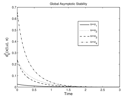
Figure 2: Convergence of mean-field to the fixed-point

13 Concluding Remarks

.

In this paper we have provided a measure-valued process approach to establish the mean-field behavior of loss systems with Power-of-$d$ routing and general service time requirements. The extension of these results to multi-class systems is also of interest and these follow in a similar manner mutatis mutandis from the approach used here. The extensions to other disciplines such as processor sharing are also of interest and the measure-valued approach used here is most appropriate. One open problem in these classes of problems is establishing the global asymptotic stability of the fixed point when unique. The standard theory does not apply as the MFEs describe a class of non-linear Markov processes on $\mathcal{R}_{+}^{n}$ without any obvious monotonicity properties and perhaps one way is to study the dissipative properties of the non-linear semi-groups of the Markov processes.

References

[1]Aghajani, R. and Ramanan, K. (2017).
The hydrodynamic limit of a randomized load balancing network.
ArXiv e-prints.
[3]Azar, Y., Broder, A. Z., Karlin, A. R. and Upfal, E. (1999).
Balanced allocations.
SIAM J. Comput.29, 180–200.
[4]Billingsley, P. (1999).
Convergence of probability measures second ed.
Wiley Series in Probability and Statistics: Probability and
Statistics. John Wiley & Sons, Inc., New York.
A Wiley-Interscience Publication.
[5]Bramson, M., Lu, Y. and Prabhakar, B. (2010).
Randomized load balancing with general service time distributions.
In Proceedings of ACM SIGMETRICS.
pp. 275–286.
[6]Bramson, M., Lu, Y. and Prabhakar, B. (2012).
Asymptotic independence of queues under randomized load balancing.
Queueing Systems71, 247–292.
[7]Brown, L., Gans, N., Mandelbaum, A., Sakov, A., Shen, H., Zeltyn, S. and
Zhao, L. (2005).
Statistical analysis of a telephone call center.
Journal of the American Statistical Association100,
36–50.
[8]Brumelle, S. L. (1978).
A generalization of erlang’s loss system to state dependent arrival
and service rates.
Mathematics of Operations Research3, 10–16.
[9]Dawson, D. A. (1993).
Measure-valued Markov processes vol. 1541 of École
d’Été de Probabilités de Saint-Flour XXI—1991.
Springer, Berlin.
[10]Decreusefond, L. and Moyal, P. (2008).
A functional central limit theorem for the m/gi/queue.
Ann. Appl. Probab.18, 2156–2178.
[11]Ethier, S. N. and Kurtz, T. G. (1985).
Markov Processes: Characterization and Convergence.
John Wiley and Sons Ltd.
[12]Graham, C. and Méléard, S. (1993).
Propagation of chaos for a fully connected loss network with
alternate routing.
Stochastic Processes and their Applications44,
159–180.
[13]Graham, C. and Méléard, S. (1997).
Stochastic particle approximations for generalized boltzmann models
and convergence estimates.
The Annals of Probability28, 115–132.
[14]Gromoll, H. C., Puha, A. L. and Williams, R. J. (2002).
The fluid limit of a heavily loaded processor sharing queue.
Ann. Appl. Probab.12, 797–859.
[15]Gromoll, H. C., Robert, P. and Zwart, B. (2008).
Fluid limits for processor-sharing queues with impatience.
Math. Oper. Res.33, 375–402.
[16]Jakubowski, A. (1986).
On the skorokhod topology.
Annales de l’I.H.P. Probabilités et Statistiques22,
263–285.
[17]Kallenberg, O. (1983).
Random measures.
Akademie-Verlag.
[18]Kang, W. and Ramanan, K. (2010).
Fluid limits of many-server queues with reneging.
Ann. Appl. Probab.20, 2204–2260.
[19]Karpelevich, F. I. and Rybko, A. N. (2000).
Thermodynamic limit for the mean field model of simple symmetrical
closed queueing network.
Markov Processes and Related Fields6, 89–105.
[20]Kaspi, H. and Ramanan, K. (2011).
Law of large numbers limits for many-server queues.
Ann. Appl. Probab.21, 33–114.
[21]Kolesar, P. (1984).
Stalking the endangered cat: A queueing analysis of congestion at
automatic teller machines.
Interfaces14, 16–26.
[22]Microsoft.
Microsoft Azure.
http://www.microsoft.com/windowsazure/.
[23]Mitzenmacher, M. (1996).
The power of two choices in randomized load balancing.
PhD Thesis, Berkeley.
[24]Mukhopadhyay, A. and Mazumdar, R. R. (2014).
Rate-based randomized routing in large heterogeneous processor
sharing systems.
In Proceedings of 26th International Teletraffic Congress (ITC
26).
[25]Mukhopadhyay, A. and Mazumdar, R. R. (2016).
Analysis of randomized join-the-shortest-queue (jsq) schemes in large
heterogeneous processor sharing systems.
IEEE Transactions on Control of Network Systems3(2),
116–126.
[26]Mukhopadhyay, A., Mazumdar, R. R. and Guillemin, F. (2015).
The power of randomized routing in heterogeneous loss systems.
In Teletraffic Congress (ITC 27), 2015 27th International.
pp. 125–133.
[27]Mukhopadhyayay, A., Karthik, A., Mazumdar, R. R. and Guillemin, F. M.
(September 2015).
Mean field and propagation of chaos in multi-class heterogeneous loss
models.
Performance Evaluation91, 117–131.
[28]Robert, P. (2003).
Stochastic Modelling and Applied Probability Series. Springer-Verlag.
[29]Rudin, W. (1987).
Real and complex analysis third ed.
McGraw-Hill Book Co., New York.
[30]Sevasta yanov, B. A. (1957).
An ergodic theorem for markov processes and its application to
telephone systems with refusals.
Theory of Probability & Its Applications2, 104–112.
[31]Turner, S. R. E. (1996).
Resource pooling in stochastic networks.
Ph.D. dissertation, University of Cambridge.
[32]Turner, S. R. E. (1998).
The effect of increasing routing choice on resource pooling.
Probability in the Engineering and Informational Sciences12, 109–124.
[33]Varadarajan, V. (1959)).
On a theorem of f. riesz concerning the form of linear functionals.
Fund. Math.46, 209–220.
[34]Vasantam, T., Mukhopadhyay, A. and Mazumdar, R. R.Mean field analysis of loss models with mixed-erlang distributions
under power-of-d routing.
Accepted for ITC 29, Genoa, Italy, Sept. 2017 2017.
[35]Vvedenskaya, N. D., Dobrushin, R. L. and Karpelevich, F. I. (1996).
Queueing system with selection of the shortest of two queues: an
asymptotic approach.
Problems of Information Transmission32, 20–34.
[36]Xie, Q., Dong, X., Lu, Y. and Srikant, R. (2015).
Power of d choices for large-scale bin packing: A loss model.
In Proceedings of the 2015 ACM SIGMETRICS.
pp. 321–334.
[37]Zhang, J. (2013).
Fluid models of many-server queues with abandonment.
Queueing Systems73, 147–193.