Contact mechanics of adhesive beams.
Part II: Low to high indentation.

Abstract

In this article, we extended our approach, that is mentioned in part 1, to model the indentation of an adhesive beam by a rigid cylindrical punch. We considered clamped and simply supported beams for this study. We first modeled these beams as infinite length elastic layers which obey the kinetic and kinematic constraints imposed by the end supports. The adhesion effects are considered via the Dugdale-Barenblatt model based adhesive zone model. Solving the governing equations of this infinite layer along with its boundary conditions, we obtain a set of coupled Fredholm integral equations of first kind. These integral equations are then solved employing the collocation technique. The results obtained are then compared with finite element (FE) simulations and the previously published results for the non-adhesive case. We also obtained the results for the well-known Johnson-Kendall-Roberts (JKR) approximation of the contact. Finally we investigated the effect of various adhesive strengths on the contact parameters and showed the transition of the results from ‘Hertzian’ to ‘JKR’ approximation.

Keywords: contact mechanics; adhesive beams; integral transforms.

1 Introduction

This article forms the second part of a three part study on the indentation of adhesive beams. In this second part we greatly expand the theoretical framework of part I (Punati et al., 2017), hereafter Paper I.

Hertz, in 1882, proposed a theory of contact of non-adhesive spheres which addressed the indentation of three dimensional half-spaces by rigid axi-symmetric punhces. Later, Johnson et al. (1971) and, Derjaguin (1934) and Derjaguin et al. (1975) proposed theories for adhesive axi-symmetric indentation. Finally, Maugis (1992) demonstrated that JKR (Johnson et al., 1971) and DMT (Derjaguin et al., 1975) theories are two limits of one general theory. Some of the above theories and the corresponding two-dimensional versions are discussed in Alexandrov and Pozharskii (2001), Galin and Gladwell (2008), Gladwell (1980), Johnson (1985), Hills et al. (1993), and Goryacheva (1998).

In recent years, indenaion of thin adhesive structures have attracted the attention of researchers because of their applications in electronics and computer industry, see e.g. Barthel and Perriot and Dalmeya et al. (2012). Some of the designs for these structural adhesives are inspired from biology, such as the one proposed by Arul and Ghatak (2008); see Fig. 1. The theoretical modeling and characterisation of such structural adhesives is of great interest. Paper I presented a step towards the modeling of structural adhesives of the type shown in Fig. 1, by investigating the indentation of adhesive beams resting on flexible supports.

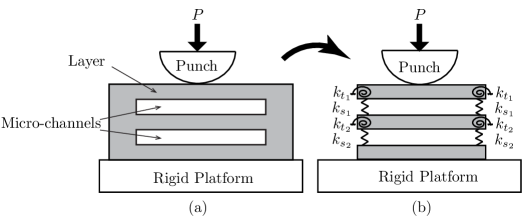
Figure 1: (a) Structural adhesive designed by Arul and Ghatak (2008). (b) Mechanical model of the structural adhesive in (a) employing an interconnected stack of adhesive beams. The rigidity of the vertical walls is modeled through torsional (stiffness $k_{t}$) and vertical translational (stiffness $k_{s}$) springs, as shown. The system is indented by a rigid punch, pressed down by the force $P$.

Indentation studies on non-adhesive beams were pursued in the past by Keer and Miller (1983), and Sankar and Sun (1983). They employed integral transforms and Fourier series, respectively. Adhesion was not considered. Recently Kim et al. (2014), revisited the indention of non-adhesive beams through approximate techniques. However, extending the methods of these papers to adhesive beams pose difficulties, as they involve several iterated integral transforms and/or asymptotic matching. Paper I presented a formulation which could address non-adhesive and adhesive contact of beams within the same framework.

In Paper I we investigated indentation by a rigid cylindrical punch of non-adhesive and adhesive beams on flexible end supports. However, the mathematical model assumed that, during indentation, the displacement of the beam’s bottom surface could be approximated by the deflection of the corresponding Euler-Bernoulli beam under the action of a point load. This approximation limited the application of Paper I’s approach to indentations where the extent $a$ of the contact region was less than or equal to the thickness $h$ of the beam. Here we release the assumption of Paper I in order to extend our framework to indentation with large contact areas. This leads naturally to a set of dual integral equations for the unknown contact pressure and the displacement of the beam’s bottom surface.

In this article, we restrict ourselves to clamped and simply supported beams which, as shown in Paper I, bound the range of behaviors displayed by beams on flexible supports.

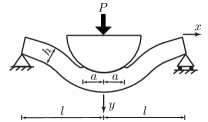
(a)

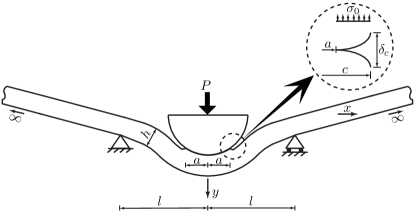
(b)

Figure 2: (a) Indentation by a rigid circular punch with an adhesive simply supported beam. (b) Mathematical model for the simply supported beam indentation by extending the beam to infinity along its slope near the ends. The inset shows the adhesive zone model employed in our mathematical formulation.

As in Paper 1, adhesion is modeled through the adhesive-zone model, which allows us to study the JKR (Johnson et al., 1971) and DMT (Derjaguin et al., 1975) approximations of adhesive contact by varying a parameter that regulates adhesive strength. Additionally, by setting adhesive strength to zero we obtain results for non-adhesive contact.

This paper is organised as follows: We first present the mathematical model, which leads to a set of dual integral equations in terms of the contact pressure and the vertical displacement of the beam’s lower surface. This is followed by non-dimensionalization and the formulation of the corresponding numerical algorithm to solve the integral equations. We then briefly discuss the FE model employed to study non-adhesive beam indentation. Next, we present and discuss results for different types of adhesive and non-adhesive contacts. Finally, we compare our predictions with preliminary experiments.

2 Mathematical model

We begin, as in Paper I, by extending the beams of Fig. 2(a) beyond the supports to infinity; see Fig. 2(b). This extension is done in keeping with the kinematic and kinetic constraints imposed by the supports. Thus, the beam is extended linearly along the slope at the supports. The beams may now be represented as a linear elastic layer of infinite length with thickness $h$, and with Young’s modulus $E$ and Poisson’s ratio $\nu$. The top and bottom surfaces of the beam are frictionless. The corresponding elasticity problem is now solved, the details of which are in Sec. 2 of Paper I. This yields the vertical displacement of the beam’s top surface $(y=0)$ and the normal traction acting on the beam’s bottom surface $(y=h)$ as, respectively,

$$v\left(x,0\right) =-\frac{2}{\pi E^{*}}\int\limits_{0}^{\infty}\bar{P}_{c}\left(\xi\right)\,K_{1}\left(\xi,x\right)\,d\xi+\frac{1}{\pi}\int\limits_{0}^{\infty}\bar{v}_{b}\left(\xi\right)\,K_{2}\left(\xi,x\right)\,d\xi$$ (2.1)

and $$\tau_{yy}\left(x,h\right) =\frac{1}{\pi}\int\limits_{0}^{\infty}\bar{P}_{c}\left(\xi\right)\,K_{2}\left(\xi,x\right)\,d\xi+\frac{{E^{*}}}{\pi}\int\limits_{0}^{\infty}\bar{v}_{b}\left(\xi\right)\,K_{3}\left(\xi,x\right)\,\cos{\xi x}\,d\xi,$$ (2.2)

where

$$\bar{P}_{c}\left(\xi\right)=\int\limits_{-\infty}^{\infty}-P_{c}\left(t\right)\cos{\xi t}\,dt\quad\text{and}\quad\bar{v}_{b}\left(\xi\right)=\int\limits_{-\infty}^{\infty}v_{b}\left(t\right)\cos{\xi t}\,dt$$ (2.3)

are the Fourier transforms of the normal force $P_{c}\left(t\right)$ acting on the beam’s top surface and the vertical displacement $v_{b}\left(t\right)$ of the beam’s bottom surface, respectively, while

$$K_{1}\left(\xi,x\right) =\frac{\sinh^{2}{\xi h}}{\xi\left(\xi h+\sinh{\xi h}\cosh{\xi h}\right)}\,\cos{\xi x},\quad K_{2}\left(\xi,x\right)=\frac{\sinh{\xi h}+\xi h\cosh{\xi h}}{\xi h+\sinh{\xi h}\cosh{\xi h}}\,\cos{\xi x}$$

and $$K_{3}\left(\xi,x\right) =\frac{\xi}{2}\cdot\frac{\sinh^{2}{\xi h}-\xi^{2}h^{2}}{\xi h+\sinh{\xi h}\cosh{\xi h}}\,\cos{\xi x}.$$

For more details see Appendix A.

To ease non-dimensionalization we expand (2.1) and (2.2) by employing definitions of $\bar{P}_{c}$ and $\bar{v}_{b}$ to obtain:

$$v\left(x,0\right) =\frac{2}{\pi E^{*}}\int\limits_{0}^{\infty}\int\limits_{-\infty}^{\infty}P_{c}\left(t\right)\cos{\xi t}\,dt\,K_{1}\left(\xi,x\right)\,d\xi+\frac{1}{\pi}\int\limits_{0}^{\infty}\int\limits_{-\infty}^{\infty}v_{b}\left(t\right)\cos{\xi t}\,dt\,K_{2}\left(\xi,x\right)\,d\xi$$ (2.4)

and $$\tau_{yy}\left(x,h\right) =\frac{1}{\pi}\int\limits_{0}^{\infty}\int\limits_{-\infty}^{\infty}-P_{c}\left(t\right)\cos{\xi t}\,dt\,K_{2}\left(\xi,x\right)\,d\xi+\frac{{E^{*}}}{\pi}\int\limits_{0}^{\infty}\int\limits_{-\infty}^{\infty}v_{b}\left(t\right)\cos{\xi t}\,dt\,K_{3}\left(\xi,x\right)\,d\xi.$$ (2.5)

In (2.5), the second integral is singular at $\xi\rightarrow\infty$. This singularity may be eliminated by integrating twice by parts, to find

$$\tau_{yy}\left(x,h\right) =\frac{1}{\pi}\int\limits_{0}^{\infty}\int\limits_{-\infty}^{\infty}-P_{c}\left(t\right)\cos{\xi t}\,dt\,K_{2}\left(\xi,x\right)\,d\xi-\frac{{E^{*}}}{\pi}\int\limits_{0}^{\infty}\int\limits_{-\infty}^{\infty}f\left(t\right)\cos{\xi t}\,dt\,\,\,\frac{1}{\xi^{2}}\,K_{3}\left(\xi,x\right)\,d\xi,$$ (2.6)

where $\kappa\left(t\right)=d^{2}v_{b}/dt^{2}$.

The contact region’s vertical displacement is fixed by the displacement of the punch $\delta$ and the profile $g(x)$ of the punch. So within the contact zone, i.e. $-a\leq x\leq a$ – where $a$ locates the contact edge - we set $v(x,0)=\delta-g(x)$. When $a$ and $\delta$ are small compared to the radius $R$ of the punch, we approximate the cylindrical profile of the punch by a parabola. Furthermore, there is no normal traction at the bottom surface of the beam, except at the supports; see Fig. 2. Thus, at the top and bottom surfaces of the layer we have, respectively,

$$v(x,0) =\delta-\frac{x^{2}}{2R}\quad\text{for}\quad-a\leq x\leq a,$$ (2.7)

and $$\tau_{yy}\left(x,h\right) =0\quad\text{for}\quad-l<x<l.$$ (2.8)

We model adhesive interaction between the punch and the beam through an adhesive-zone (Maugis, 1992). The normal tractions within the adhesive zone follow the Dugdale-Barenblatt model, in which a constant attractive force $\sigma_{0}$ acts per unit length within the adhesive zone of length $d=c-a$, where $c$ demarcates the adhesive zone’s outer edge, see inset in Fig. 2(b). With this we write the normal traction on the top surface as

$$P_{c}\left(x\right)=\left\{\begin{array}[]{ll}p\left(x\right)&\quad\text{for }\,|x|\leq a,\\ -\sigma_{0}&\quad\text{for }\,a\leq|x|\leq c,\\ 0&\quad\text{for }\,|x|>c.\end{array}\right.$$ (2.9)

An adhesive-zone model resolves stress singularities at the contact edges ($x=\pm a$) inherent in the JKR approximation by requiring the normal traction be continuous there, i.e.,

$$\lim_{x\rightarrow\pm a^{\mp}}p\left(x\right)=-\sigma_{0}.$$ (2.10)

An adhesive zone introduces the extra variable $c$ into the contact problem. The required additional equation is obtained by equating the energy release rate $G$ – computed employing the $J-$Integral (Rice, 1968) – to the work of adhesion $w$, to obtain the energy balance

$$\sigma_{0}\delta_{c}=w,$$ (2.11)

where

$$\delta_{c}=\left(c^{2}/2R\right)-\delta+v_{c}$$ (2.12)

is the air gap at the end of the adhesive zone (see inset in Fig. 2(b)) and $v_{c}=v\left(c,0\right)$ is the vertical displacement of the top surface at $x=c$.

In non-adhesive indentation, $\sigma_{0}=0=w$, and (2.11) is automatically satisfied. When the JKR approximation is invoked, $\sigma_{0}\rightarrow\infty$ and $c\rightarrow a$, so that employing the Griffith’s criterion (2.11) becomes

$$\frac{K_{1}^{2}}{2E^{*}}=w,$$ (2.13)

where

$$K_{1}=-\lim_{x\rightarrow a^{-}}\sqrt{2\pi\left(a-x\right)}p\left(x\right)$$ (2.14)

is the stress intensity factor; see e.g. Kanninen and Popelar (1985, p. 168). Note that the continuity condition (2.10) is redundant for the JKR approximation.

Finally, the total load acting on the punch is

$$P=\int\limits_{-\infty}^{\infty}P_{c}\left(x\right)\,dx=\int\limits_{-a}^{a}p\left(x\right)dx-2\,\sigma_{0}\left(c-a\right).$$ (2.15)

3 Non-dimensionalization

We generally follow the non-dimensionalization of Paper I:

$$A=\frac{a}{l};\quad\varphi\left(\bar{\tau}\right)=\frac{aRl}{Kh^{3}}\,p\left(a\bar{\tau}\right);\quad\bar{P}=\frac{PRl}{Kh^{3}};$$

$$\Delta=\frac{\delta R}{l^{2}};\quad L=\frac{l}{R};\quad\lambda=2\sigma_{0}\left(\frac{R}{\pi wK^{2}}\right)^{1/3};\quad m=\left(\frac{\pi w}{RK}\right)^{1/3},$$

where $K=4\,E^{*}/3$. The variables are scaled as

$$\left\{\bar{x},\bar{\tau},\bar{c},\bar{l},\bar{\gamma}\right\}=\frac{1}{a}\left\{x,t,c,l,h\right\};\quad\left\{\hat{\tau},\hat{\gamma}\right\}=\frac{1}{l}\left\{t,h\right\};\quad\left\{\omega,\bar{\omega},\hat{\omega}\right\}=\left\{\xi h,\frac{\omega}{\bar{\gamma}},\frac{\omega}{\hat{\gamma}}\right\};$$

$$\Phi\left(\tau\right)=\frac{aRl}{Kh^{3}}\,P\left(a\bar{\tau}\right);\quad\vartheta_{b}\left(\hat{\tau}\right)=v_{b}\left(\hat{\tau}\right)\,\left(\frac{R}{l^{2}}\right);\quad\kappa_{b}\left(\hat{\tau}\right)=\frac{d^{2}\vartheta_{b}\left(\hat{\tau}\right)}{d\hat{\tau}^{2}};\quad\mathcal{T}=\frac{\tau_{yy}\left(\hat{x},h\right)}{K}\frac{8\hat{\gamma}}{3L}.$$

Employing the above, the non-dimensional vertical displacement of the top surface (2.4) and the normal traction at the bottom surface (2.6) become, respectively,

$$\vartheta\left(\bar{x},0\right) =\frac{8\hat{\gamma}^{3}}{3\pi}\int\limits_{0}^{\infty}\int\limits_{-\infty}^{\infty}\Phi\left(\bar{\tau}\right)\cos\left(\bar{\omega}\tau\right)\,d\bar{\tau}\,K^{t}_{1}\left(\bar{\omega},\bar{x}\right)d\omega+\frac{1}{\pi\hat{\gamma}}\int\limits_{0}^{\infty}\int\limits_{-\infty}^{\infty}\vartheta_{b}\left(\hat{\tau}\right)\cos\left(\hat{\omega}\hat{\tau}\right)\,d\hat{\tau}\,K^{t}_{2}\left(\bar{\omega},\bar{x}\right)d\omega$$ (3.1)

$$\text{and}\quad\mathcal{T} =\frac{8\hat{\gamma}^{3}}{3\pi}\int\limits_{0}^{\infty}\int\limits_{-\infty}^{\infty}-\Phi\left(\bar{\tau}\right)\cos\left(\bar{\omega}\bar{\tau}\right)\,d\bar{\tau}\,K^{b}_{1}\left(\hat{\omega},\hat{x}\right)d\omega-\frac{\hat{\gamma}}{\pi}\int\limits_{0}^{\infty}\int\limits_{-\infty}^{\infty}\kappa_{b}\left(\hat{\tau}\right)\cos\left(\hat{\omega}\hat{\tau}\right)\,d\hat{\tau}\,K^{b}_{2}\left(\hat{\omega},\hat{x}\right)d\omega,$$ (3.2)

where the kernels

$$K^{t}_{1}\left(\bar{\omega},\bar{x}\right) =\frac{\sinh^{2}{\omega}}{\omega\left(\omega+\sinh{\omega}\cosh{\omega}\right)}\,\cos\left(\bar{\omega}\bar{x}\right), \quad K^{t}_{2}\left(\bar{\omega},\bar{x}\right) =\frac{\sinh{\omega}+\omega\cosh{\omega}}{\omega+\sinh{\omega}\cosh{\omega}}\,\cos\left(\bar{\omega}\bar{x}\right),$$

$$K^{b}_{1}\left(\hat{\omega},\hat{x}\right) =\frac{\sinh{\omega}+\omega\cosh{\omega}}{\omega+\sinh{\omega}\cosh{\omega}}\,\cos\left(\hat{\omega}\hat{x}\right)\quad\text{and} \quad K^{b}_{2}\left(\hat{\omega},\bar{x}\right) =\frac{1}{\omega}\cdot\frac{\sinh^{2}{\omega}-\omega^{2}}{\omega+\sinh{\omega}\cosh{\omega}}\,\cos\left(\hat{\omega}\hat{x}\right).$$ (3.3)

Non-dimensionalizing (2.7) – (2.11) yields

$$\vartheta(\bar{x},0) =\Delta-\frac{1}{2}\,\bar{x}^{2}A^{2}\quad\text{for}\quad-1\leq\bar{x}\leq 1,$$ (3.4)

$$\mathcal{T}\left(\hat{x},h\right) =0\quad\text{for}\quad-1<\hat{x}<1,$$ (3.5)

$$\Phi\left(\bar{\tau}\right) =\left\{\begin{array}[]{ll}\varphi\left(\bar{\tau}\right),&\quad-1\leq\bar{\tau}\leq 1\\ -\lambda Am/2\hat{\gamma}^{3}L,&\quad 1\leq|\bar{\tau}|\leq\bar{c}\\ 0,&\quad|\bar{\tau}|>\bar{c}\end{array}\right.$$ (3.9)

$$\varphi\left(\pm 1\right) =-\frac{\lambda Am}{2\hat{\gamma}^{3}L}$$ (3.10)

and $$1 =\frac{\pi\lambda L^{2}}{2m^{2}}\,\left(\frac{1}{2}\,\bar{c}^{2}\,A^{2}-\Delta+\vartheta_{c}\right),$$ (3.11)

where $\vartheta\left(\bar{c}\right)=\vartheta\left(\bar{c},0\right)$, and $\Delta=\vartheta\left(0,0\right)$. In the JKR approximation, we replace (3.10) and (3.11) by the non-dimensional Griffith’s criterion, obtained from (2.13) and (2.14):

$$\lim_{\bar{x}\rightarrow 1^{-}}\sqrt{\left(1-\bar{x}\right)}\varphi\left(\bar{x}\right)=-\frac{m}{2\pi L}\left(\frac{l}{h}\right)^{3}\sqrt{\frac{3Am}{L}}.$$ (3.12)

Substituting (3.9) in (3.1) and (3.2) yields

$$\vartheta\left(\bar{x},0\right)= -\frac{8\hat{\gamma}^{3}}{3\pi}\int\limits_{0}^{\infty}\bar{\varphi}\left(\bar{\omega}\right)K^{t}_{1}\left(\bar{\omega},\bar{x}\right)d\omega-\frac{8\lambda Am}{3\pi L}\int\limits_{0}^{\infty}\bar{\varphi}_{0}\left(\bar{\omega}\right)K^{t}_{1}\left(\bar{\omega},\bar{x}\right)d\omega+\frac{1}{\pi\hat{\gamma}}\int\limits_{0}^{\infty}\hat{\vartheta}_{b}\left(\hat{\omega}\right)K^{t}_{2}\left(\bar{\omega},\bar{x}\right)d\omega,$$ (3.13)

and

$$\mathcal{T}= \frac{8\hat{\gamma}^{3}}{3\pi}\int\limits_{0}^{\infty}\bar{\varphi}\left(\bar{\omega}\right)K^{b}_{1}\left(\hat{\omega},\hat{x}\right)d\omega+\frac{8\lambda Am}{3\pi L}\int\limits_{0}^{\infty}\bar{\varphi}_{0}\left(\bar{\omega}\right)K^{b}_{1}\left(\hat{\omega},\hat{x}\right)d\omega-\frac{\hat{\gamma}}{\pi}\int\limits_{0}^{\infty}\hat{\kappa}_{b}\left(\hat{\omega}\right)K^{b}_{2}\left(\hat{\omega},\hat{x}\right)d\omega,$$ (3.14)

with

$$\begin{aligned} \bar{\varphi}\left(\bar{\omega}\right)&=-\int\limits_{-1}^{1}\varphi\left(\bar{\tau}\right)\cos{\bar{\omega}\,\bar{\tau}}\,d\bar{\tau},&\quad\bar{\varphi}_{0}\left(\bar{\omega}\right)&=\int\limits_{1}^{\bar{c}}\cos{\bar{\omega}\,\bar{\tau}}\,d\bar{\tau},\\ \hat{\vartheta}_{b}\left(\hat{\omega}\right)&=\int\limits_{-\infty}^{\infty}\vartheta_{b}\left(\hat{\tau}\right)\cos{\hat{\omega}\hat{\tau}}\,d\hat{\tau}\quad\text{and }&\quad\hat{\kappa}_{b}\left(\hat{\omega}\right)&=\int\limits_{-\infty}^{\infty}\kappa_{b}\left(\hat{\tau}\right)\cos{\hat{\omega}\hat{\tau}}\,d\hat{\tau}.\end{aligned}$$

Then, combining (3.13) with (3.4), and (3.14) with (3.5), we obtain

$$\Delta-\frac{1}{2}\,\bar{x}^{2}A^{2}= -\frac{8\hat{\gamma}^{3}}{3\pi}\int\limits_{0}^{\infty}\bar{\varphi}\left(\bar{\omega}\right)\,K^{t}_{1}\left(\bar{\omega},\bar{x}\right)\,\,d\omega-\frac{8\lambda Am}{3\pi L}\int\limits_{0}^{\infty}\bar{\varphi}_{0}\left(\bar{\omega}\right)\,K^{t}_{1}\left(\bar{\omega},\bar{x}\right)\,\,d\omega$$

$$+\frac{1}{\pi\hat{\gamma}}\int\limits_{0}^{\infty}\hat{\vartheta}_{b}\left(\hat{\omega}\right)\,K^{t}_{2}\left(\bar{\omega},\bar{x}\right)\,\,d\omega\quad\text{for }-1\leq\bar{x}\leq 1$$ (3.15)

and $$0= -\frac{8\hat{\gamma}^{3}}{3\pi}\int\limits_{0}^{\infty}\bar{\varphi}\left(\bar{\omega}\right)\,K^{b}_{1}\left(\hat{\omega},\hat{x}\right)\,\,d\omega-\frac{8\lambda Am}{3\pi L}\int\limits_{0}^{\infty}\bar{\varphi}_{0}\left(\bar{\omega}\right)\,K^{b}_{1}\left(\hat{\omega},\hat{x}\right)\,\,d\omega$$

$$+\frac{\hat{\gamma}}{\pi}\int\limits_{0}^{\infty}\hat{\kappa}_{b}\left(\hat{\omega}\right)\,K^{b}_{2}\left(\hat{\omega},\hat{x}\right)\,\,d\omega\quad\text{for }-1<\hat{x}<1.$$ (3.16)

Finally, the total non-dimensional load acting on the punch is given by

$$\bar{P}=\int\limits_{-1}^{1}\varphi\left(\bar{\tau}\right)\,d\bar{\tau}-\frac{\lambda Am}{\hat{\gamma}^{3}L}\left(\bar{c}-1\right).$$ (3.17)

Equations (3) and (3) are coupled Fredholm integral equations of the first kind; see Polyanin and Manzhirov (2008, p. 573). These, along with (3.10) and (3.11), are to be solved for $\bar{\varphi}$, $\bar{\vartheta}$ and $\Delta$ for a given contact area $A$. The numerical algorithm employed for this is discussed next.

4 Numerical solution

The dual integral equations (3) and (3) cannot be solved in closed form due to the presence of complex kernels; cf. 3.3. We, therefore employ a numerical solution.

We begin by approximating the contact pressure $\varphi$ as

$$\varphi\left(\bar{\tau}\right)=\frac{-\lambda Am}{2\hat{\gamma}^{3}L}+\frac{1}{\sqrt{\left(1-\bar{\tau}^{2}\right)}}\sum_{n=0}^{N}b_{2n}T_{2n}\left(\bar{\tau}\right)\quad\text{for }-1\leq\bar{\tau}\leq 1,$$ (4.1)

where $T_{2n}\left(\bar{\tau}\right)$ are Chebyshev polynomials of the first kind and $b_{2n}$ are constants that are to be determined. Only even Chebyshev polynomials are considered as the indentation is symmetric about $\bar{\tau}=0$. The constant term is chosen to account for the contact pressure at the contact edge in the adhesive-zone model explicitly. Evaluating the integrals $\bar{\varphi}\left(\bar{\omega}\right)$ and $\hat{\varphi}\left(\bar{\omega}\right)$ in (3) after employing (4.1) yields

$$\bar{\varphi}\left(\bar{\omega}\right)=\frac{\lambda Am}{\hat{\gamma}^{3}L}\,\frac{\sin{\bar{\omega}}}{\bar{\omega}}-\sum_{n=0}^{N}b_{2n}\alpha_{2n}\left(\bar{\omega}\right)\quad\text{and}\quad\bar{\varphi}_{0}\left(\bar{\omega}\right)=\frac{1}{\bar{\omega}}\,\left(-\sin{\bar{\omega}}+\sin{\bar{\omega}\,\bar{c}}\right),$$ (4.2)

where

$$\alpha_{2n}\left(\bar{\omega}\right)=\int\limits_{-1}^{1}\frac{1}{\sqrt{\left(1-\bar{\tau}^{2}\right)}}T_{2n}\left(\bar{\tau}\right)\cos{\bar{\omega}\bar{\tau}}\>\>d\bar{\tau}.$$ (4.3)

The evaluation of the integrals $\alpha_{2n}\left(\bar{\omega}\right)$ at different $n$ are available in the appendix of Paper I.

Next, we approximate the displacement of the bottom surface $\vartheta_{b}\left(\hat{\tau}\right)$ in a series of the natural mode shapes $S_{n}\left(\hat{\tau}\right)$ of the beam:

$$\vartheta_{b}\left(\hat{\tau}\right)=d_{0}+\sum_{n=1}^{N}d_{n}\,S_{n}\left(\hat{\tau}\right).$$ (4.4)

We note that $S_{n}\left(\hat{\tau}\right)=\cos\left(n\pi\hat{\tau}\right)$ and $S_{n}\left(\hat{\tau}\right)=\sin\left\{\left(2n-1\right)\pi\left(\hat{\tau}+1\right)/2\right\}$ for clamped and simply supported beams, respectively. After these approximations are made to satisfy the beam’s end conditions, the curvature $\kappa_{b}$ of the beam is calculated from $\vartheta_{b}$. The details of these calculations are available in Appendices B and C. From (C.6) we find that the Fourier transforms $\hat{\vartheta}_{b}\left(\hat{\omega}\right)$ and $\hat{\kappa}_{b}\left(\hat{\omega}\right)$, for both clamped and simply supported beams, may be written as

$$\hat{\vartheta}_{b}\left(\hat{\omega}\right)=\sum_{n=1}^{M}d_{n}\hat{\beta}_{n}\left(\hat{\omega}\right)\quad\text{and}\quad\hat{\kappa}_{b}\left(\hat{\omega}\right)=\sum_{n=1}^{M}d_{n}\hat{\kappa}_{n}\left(\hat{\omega}\right),$$ (4.5)

where the expressions for $\hat{\beta}_{n}$ and $\hat{\kappa}_{n}$ are provided in Appendix C.

Substituting (4.2) and (4.5) in the integral equations (3) and (3) yields, respectively,

$$\Delta-\frac{1}{2}\,\bar{x}^{2}A^{2} =\frac{8\hat{\gamma}^{3}}{3\pi}\sum_{n=0}^{N}b_{2n}\mathcal{J}^{t}_{2n}\left(\bar{x}\right)-\frac{8\lambda Am}{3\pi L}\mathcal{J}^{t}\left(\bar{x}\right)+\frac{1}{\pi\hat{\gamma}}\sum_{n=1}^{M}d_{n}\mathcal{Q}^{t}_{n}\left(\bar{x}\right)$$ (4.6)

and $$0 =\frac{8\hat{\gamma}^{3}}{3\pi}\sum_{n=0}^{N}b_{2n}\mathcal{J}^{b}_{2n}\left(\hat{x}\right)-\frac{8\lambda Am}{3\pi L}\mathcal{J}^{b}\left(\hat{x}\right)+\frac{\hat{\gamma}}{\pi}\sum_{n=1}^{M}d_{n}\mathcal{Q}^{b}_{n}\left(\hat{x}\right),$$ (4.7)

where

$$\mathcal{J}^{t}_{2n}\left(\bar{x}\right) =\int\limits_{0}^{\infty}\alpha_{2n}\left(\bar{\omega}\right)\,K^{t}_{1}\left(\bar{\omega},\bar{x}\right)\,\,d\omega, \quad\mathcal{J}^{t}\left(\bar{x}\right) =\int\limits_{0}^{\infty}\frac{1}{\bar{\omega}}\,\sin\left(\bar{\omega}\,\bar{c}\right)\,K^{t}_{1}\left(\bar{\omega},\bar{x}\right)\,\,d\omega,$$

$$\mathcal{Q}^{t}_{n}\left(\bar{x}\right) =\int\limits_{0}^{\infty}\hat{\beta}_{n}\left(\hat{\omega}\right)\,K^{t}_{2}\left(\bar{\omega},\bar{x}\right)\,\,d\omega, \quad\mathcal{Q}^{b}_{n}\left(\hat{x}\right) =\int\limits_{0}^{\infty}\hat{\kappa}_{n}\left(\hat{\omega}\right)\,K^{b}_{2}\left(\hat{\omega},\hat{x}\right)\,\,d\omega,$$

$$\mathcal{J}^{b}_{2n}\left(\hat{x}\right) =\int\limits_{0}^{\infty}\alpha_{2n}\left(\bar{\omega}\right)\,K^{b}_{1}\left(\hat{\omega},\hat{x}\right)\,\,d\omega \text{and}\quad\quad\mathcal{J}^{b}\left(\bar{x}\right) =\int\limits_{0}^{\infty}\frac{1}{\bar{\omega}}\,\sin\left(\bar{\omega}\,\bar{c}\right)\,K^{b}_{1}\left(\hat{\omega},\hat{x}\right)\,\,d\omega.$$

The above integrals may be evaluated at any $\bar{x}$ or $\hat{x}$ through the Clenshaw-Curtis quadrature; see Press et al. (1992, p. 196).

Employing (4.1), the constraint (3.10) on the contact pressure at the ends of the contact region provides

$$b_{0}+b_{2}+\cdots+b_{2N}=0.$$ (4.8)

Utilizing the approximations (4.2) and (4.5), the energy balance equation (3.11) yields

$$\frac{\pi\lambda L^{2}}{2m^{2}}\,\left(\frac{1}{2}\,\bar{c}^{2}\,A^{2}-\Delta+\vartheta_{c}\right)=1,$$ (4.9)

with

$$\vartheta\left(\bar{c}\right)= \frac{8\hat{\gamma}^{3}}{3\pi}\sum_{n=0}^{N}b_{2n}\mathcal{J}^{t}_{2n}\left(\bar{c}\right)-\frac{8\lambda Am}{3\pi L}\mathcal{J}^{t}\left(\bar{c}\right)+\frac{1}{\pi\hat{\gamma}}\sum_{n=1}^{M}d_{n}\mathcal{Q}^{t}_{n}\left(\bar{c}\right),$$ (4.10)

where $\Delta$ is the displacement of the punch. We recall that the energy balance (4.9) is redundant for the case of adhesionless contact or when the JKR approximation is invoked.

Finally, the total load acting on the punch becomes after employing (2.8) and (4.1):

$$\bar{P}=\pi b_{0}-\frac{\lambda Am}{\hat{\gamma}^{3}L}\bar{c}.$$ (4.11)

5 Algorithm

We need to solve (4.6) – (4.9) for the $N+M+3$ unknowns $b_{2n}$, $d_{n}$, $\Delta$ and $\bar{c}$ at any given contact area $A$. These are solved through the collocation technique (Atkinson1997Inteqns, p. 135), which provides the necessary $N+M+3$ algebraic equations.

In the collocation method, (4.6) and (4.7) are required to hold exactly at, respectively, $N+1$ and $M$ collocation points. The collocation points for (4.6) and (4.7) are selected to be

$$\bar{x}_{i} =\cos\left\{\frac{\left(2i-1\right)\pi}{2\left(N+1\right)}\right\}\text{ for }i=1,\cdots,N+1,$$

and $$\hat{x}_{k} =\frac{k-1}{M}\text{ for }k=1,\cdots,M,$$

respectively. Here, $\bar{x}_{i}$ are the $N+1$ zeros of the (Chebyshev) polynomials $T_{2N+2}(\bar{x}_{i})$ (Mason and Handscomb, 2003, p. 19), while $\hat{x_{k}}$ are simply equally spaced points lying between $0$ and $1$. At these collocation points (4.6) and (4.7) become, respectively,

$$\Delta-\frac{1}{2}\,\bar{x}^{2}_{i}A^{2}= \frac{8\hat{\gamma}^{3}}{3\pi}\sum_{n=0}^{N}b_{2n}\mathcal{J}^{t}_{2n}\left(\bar{x}_{i}\right)-\frac{8\lambda Am}{3\pi L}\mathcal{J}^{t}\left(\bar{x}_{i}\right)+\frac{1}{\pi\hat{\gamma}}\sum_{n=1}^{M}d_{n}\mathcal{Q}^{t}_{n}\left(\bar{x}_{i}\right)$$ (5.1)

and $$0= \frac{8\hat{\gamma}^{3}}{3\pi}\sum_{n=0}^{N}b_{2n}\mathcal{J}^{b}_{2n}\left(\hat{x}_{k}\right)-\frac{8\lambda Am}{3\pi L}\mathcal{J}^{b}\left(\hat{x}_{k}\right)+\frac{\hat{\gamma}}{\pi}\sum_{n=1}^{M}d_{n}\mathcal{Q}^{b}_{n}\left(\hat{x}_{k}\right),$$ (5.2)

with $i=1,\cdots,N+1$ and $k=1,\cdots,M$. Thus, we obtain $N+1$ equations from (5.1) and $M$ equations from (5.2) for a total of $N+M+1$ equations. Along with (4.8) and (4.9), we finally obtain the required $N+M+3$ equations to solve for the $N+1$ unknowns $b_{2n}$, M unknowns $d_{n}$, $\Delta$ and $\bar{c}$. This system of non-linear algebraic equations is solved for any given contact area $A$ through the following algorithm:

1. For the given contact area $A$, we make an initial guess for $\bar{c}$.

2. We then write (5.1) and (5.2) in matrix notation as

   $$\Delta\,\underline{e}-\underline{f}-\underline{\lambda}=\underline{\underline{R}}\,\underline{a},$$ (5.3)

   where

   $$\underline{e}=\left[\underline{e}^{t},\underline{e}^{b}\right]^{\text{T}};\quad\underline{f}=\left[\underline{f}^{t},\underline{f}^{b}\right]^{\text{T}};\quad\underline{\lambda}=\left[\underline{\lambda}^{t},\underline{\lambda}^{b}\right]^{\text{T}};\quad\underline{a}=\left[\underline{a}^{t},\underline{a}^{b}\right]^{\text{T}};\quad\underline{\underline{R}}=\left[\begin{array}[]{cc}\underline{\underline{\mathcal{J}}}^{t}&\underline{\underline{\mathcal{Q}}}^{t}\\ \underline{\underline{\mathcal{J}}}^{b}&\underline{\underline{\mathcal{Q}}}^{b}\end{array}\right],$$ (5.6)

   with

   $$a^{t}_{i}=b_{2i-2};\,a^{b}_{k}=d_{k};\quad e^{t}_{i}=1;\,e^{b}_{k}=0;\quad f^{t}_{i}=\frac{x_{i}^{2}A^{2}}{2};\quad f^{b}_{k}=0;$$

   $$\lambda^{t}_{i}=-\frac{8\lambda Am}{3\pi L}\mathcal{J}^{t}\left(\bar{x}_{i}\right);\quad\lambda^{b}_{k}=-\frac{8\lambda Am}{3\pi L}\mathcal{J}^{b}\left(\hat{x}_{k}\right);\quad\mathcal{J}^{t}_{i\,j}=\frac{8\hat{\gamma}^{3}}{3\pi}\mathcal{J}^{t}_{2j-2}\left(\bar{x}_{i}\right);$$

   $$\mathcal{Q}^{t}_{i\,r}=\frac{1}{\pi\hat{\gamma}}\mathcal{Q}^{t}_{r}\left(\bar{x}_{i}\right);\quad\mathcal{J}^{b}_{k\,j}=\frac{8\hat{\gamma}^{3}}{3\pi}\mathcal{J}^{b}_{2j-2}\left(\hat{x}_{k}\right);\quad\mathcal{Q}^{b}_{i\,r}=\frac{\hat{\gamma}}{\pi}\mathcal{Q}^{b}_{r}\left(\hat{x}_{k}\right),$$ (5.7)

   for $i,j=1,2,\cdots,N+1$ and $k,r=1,2,\cdots,M$. Thus, $\underline{e}$, $\underline{f}$, $\underline{\lambda}$, $\underline{a}$ are column vectors of size $N+M+1$, and $\underline{\underline{R}}$ is a matrix of size $(N+M+1)\times(N+M+1)$.

3. Note that the column vector $\underline{a}$ consists of the coefficients occurring in expressions (4.1) for the contact pressure and (4.4) for the displacement. We now invert (5.3) to find $\underline{a}$ in terms of $\Delta$:

   $$\underline{a}=\Delta\underline{E}-\underline{F}-\underline{\Lambda},$$ (5.8)

   where

   $$\underline{E}=\underline{\underline{R}}^{-1}\cdot\underline{e},\quad\underline{F}=\underline{\underline{R}}^{-1}\cdot\underline{f}\quad\text{and}\quad\underline{\Lambda}=\underline{\underline{R}}^{-1}\cdot\underline{\lambda}\,.$$

4. Employing the end condition (4.8) for the contact pressure, we obtain the punch’s displacement

   $$\Delta=\frac{p_{0}+\sum_{i=1}^{N+1}F_{i}+\sum_{i=1}^{N+1}\Lambda_{i}}{\sum_{i=1}^{N+1}E_{i}},$$ (5.9)

   where

   $$p_{0}=\left\{\begin{array}[]{l}0\quad\text{ if there is no adhesion or an adhesive zone is present},\\ -\left({m\sqrt{6Am}}/{2\pi L^{2}}\right)\left({l}/{h}\right)^{3}\quad\text{ if the JKR approximation is invoked}.\end{array}\right.$$ (5.10)

5. Once $\Delta$ is known, we evaluate $\underline{a}$ from (5.8) through

   $$\underline{a}=\left(\frac{p_{0}+\sum_{i=1}^{N+1}F_{i}+\sum_{i=1}^{N+1}\Lambda_{i}}{\sum_{i=1}^{N+1}E_{i}}\right)\underline{E}-\underline{F}-\underline{\Lambda}.$$ (5.11)

6. Employing $\Delta$ and $\underline{a}$, we calculate the displacement of the beam’s top surface at $\bar{c}$ from (4.10) and check whether (4.9) holds. If not, then we update $\bar{c}$ employing the Newton-Raphson method (Chatterjee, 2002). Steps 1-6 are repeated until (4.9) is satisfied. Steps 1 and 6 are required only when we employ an adhesive zone. When the Hertzian or JKR approximations are invoked we may conveniently skip this Step 6.

7. We finally proceed to find the contact pressure distribution $\varphi\left(\bar{\tau}\right)$ and the total load $\bar{P}$ from (4.1) and (4.11), respectively.

6 Finite element (FE) computations

Finite element (FE) computations are carried out for clamped and simply supported beams for adhesionless contact. These are employed to validate our semi-analytical results.

The FE model is prepared in ABAQUS as described in Paper I: the beam is modelled as a linear elastic layer of Young’s modulus $E=2000$ MPa, Poisson’s ratio $\nu=0.3$, thickness $h=4$ mm, and half-span $l=40$ mm. The rigid punch is modeled as a much stiffer elastic material with Young’s modulus $E_{p}=2\times 10^{6}$ MPa and radius $R=225$ mm. Plane-strain elements are considered both for the beam and the punch. A concentrated load is applied on the punch. Computations provide the contact pressure $\varphi$, contact area $A$, punch’s displacement $\Delta$, and the displacement $\vartheta_{b}$ of the beam’s bottom surface.

7 Results: Non-adhesive (‘Hertzian’) contact

We now report results for the non-adhesive interaction of clamped and simply supported beams with a rigid cylindrical punch.

For non-adhesive interaction, we set $\lambda=0$ in (4.6) and (4.7) to obtain

$$\Delta-\frac{1}{2}\,\bar{x}^{2}A^{2} =\frac{8\hat{\gamma}^{3}}{3\pi}\sum_{n=0}^{N}b_{2n}\mathcal{J}^{t}_{2n}\left(\bar{x}\right)+\frac{1}{\pi\hat{\gamma}}\sum_{n=1}^{M}d_{n}\mathcal{Q}^{t}_{n}\left(\bar{x}\right)$$ (7.1)

and $$0 =\frac{8\hat{\gamma}^{3}}{3\pi}\sum_{n=0}^{N}b_{2n}\mathcal{J}^{b}_{2n}\left(\hat{x}\right)+\frac{\hat{\gamma}}{\pi}\sum_{n=1}^{M}d_{n}\mathcal{Q}^{b}_{n}\left(\hat{x}\right),$$ (7.2)

respectively. In non-adhesive contact, the interacting surfaces detach smoothly at the contact edges, so that the pressure vanishes at the contact edge, and (4.8) holds, i.e.

$$b_{0}+b_{2}+\cdots+b_{2N} = 0.$$ (7.3)

We proceed to solve (7.1) – (7.3) through the procedure of Sec. 5. We set $N=5$ and $M=50$ in our computations. Initially to compare our results with FE computations we employ the parameters of Sec. 6.

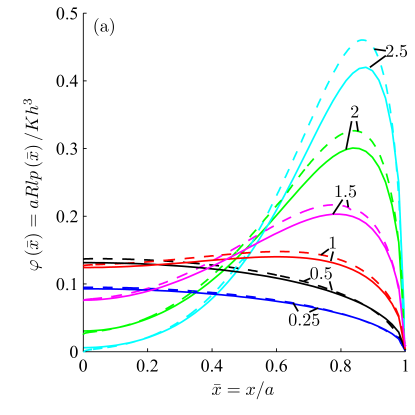
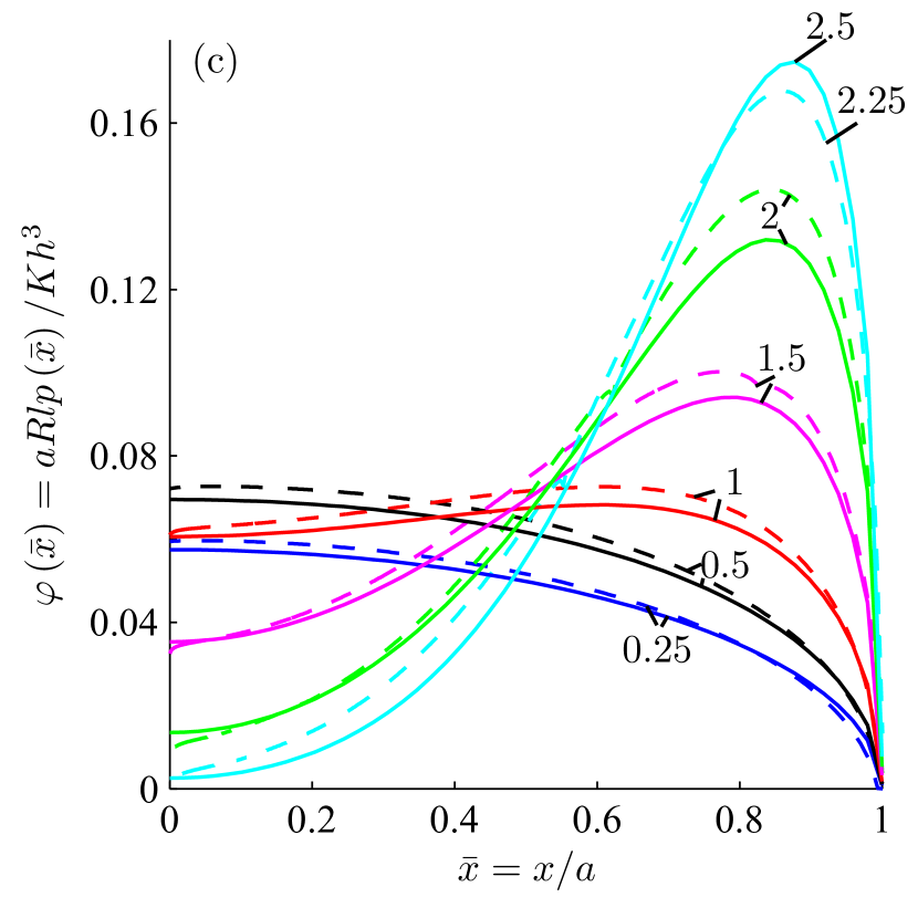
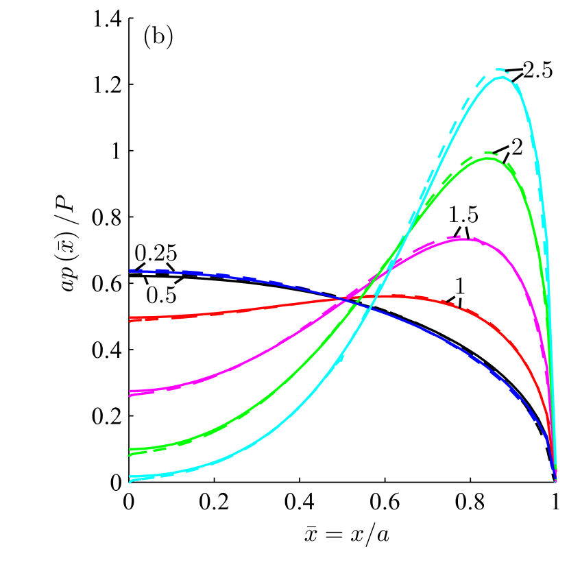
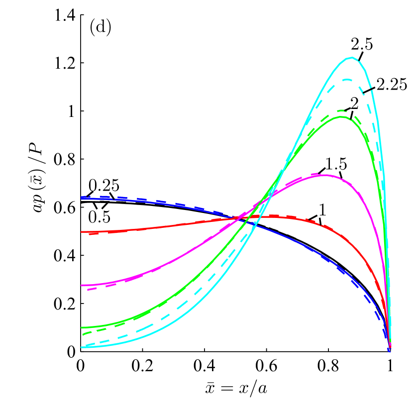
Figure 3: The non-dimensional contact pressures $\varphi\left(\bar{x}\right)$ and $ap\left(\bar{x}\right)/P$ during the non-adhesive indentation of a clamped (a and b) and simply supported (c and d) beams. We set $h=4$ mm and $l=40$ mm. Several contact areas $a$ are investigated by varying $a/h$ ratio, which are noted next to then corresponding curves. The solid lines are results obtained from the semi-analytical procedure of Sec. 4, while dashed line represent FE computations.

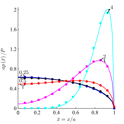
(a)

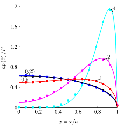
(b)

Figure 4: The non-dimensional contact pressures $ap\left(\bar{x}\right)/P$ during the non-adhesive indentation of (a) a clamped and (b) a simply beam. The slenderness ratio of the beam $l/h=10$. Several contact areas $a$ are investigated by varying $a/h$ ratio, which are noted next to then corresponding curves. The solid lines are results obtained from the semi-analytical procedure of Sec. 4. Dots represent the predictions of Keer and Miller (1983).

Figure 3 plots $\varphi\left(\bar{x}\right)$ and $ap\left(\bar{x}\right)$, computed by solving (7.1) – (7.3) and from FE simulations. Results for both clamped and simply supported beams are shown. These pressure profiles are plotted at different $a/h$ ratios, by varying the contact area $a$, for a beam of thickness $h$ and half-span $l$. We observe that at low $a/h$ ratios, the contact pressure is maximum at the center of the contact area and vanishes as we approach the contact edges. Increasing $a/h$ causes the contact pressure to decrease at the center of the contact area and increase near its ends. This behavior was also observed in Paper I.

As in Paper I, we find that, at the same $a/h$, the contact pressure $\varphi$ in a simply supported beam is smaller than that in a clamped beam, because the bending stiffness of the former is lower. However, this difference is not reflected when we plot $ap\left(\bar{x}\right)$; cf. Figs. 3(b) and 3(d) . We observe a close match between our predictions and FE simulations for all $a/h$, except for a small deviation between the two at $a/h=2.5$ in the case of simply supported beams. We suspect that the latter may be due to the shear-free boundary condition at the top and bottom surface of the beam that was employed in the theoretical model but is not imposed in the FE model. We note that method of Paper I does well until $a/h\approx 1$. With greater indentation, the $a/h$ ratio increases, and the contact pressure at the center of the contact patch becomes negative. This reflects loss of contact, which is observed in both theoretical predictions and FE computations. For clamped beams, contact loss initiates at the center of the contact area when $a/h\gtrsim 2.5$. In simply supported beams contact loss is predicted for $a/h\gtrsim 2.5$ by our analytical model but for $a/h\gtrsim 2.25$ by FE simulations.

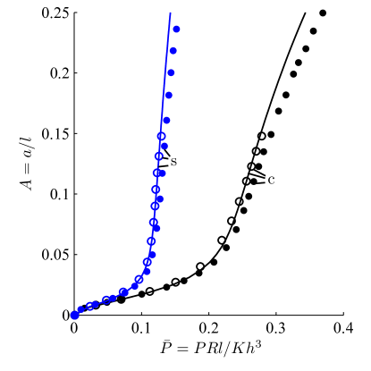
(a)

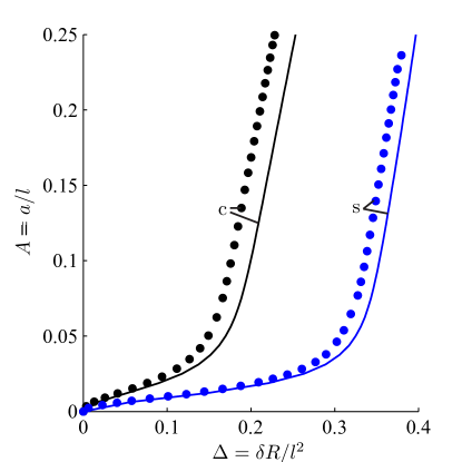
(b)

Figure 5: Non-adhesive contact of clamped (‘c’) and simply supported (‘s’) beams. The contact area $A$ is plotted as a function of (a) the total load $\bar{P}$ acting on the punch and (b) the punch’s displacement $\Delta$. The beam’s slenderness ratio $l/h$=10. Solid lines are results obtained from the semi-analytical procedure of Sec. 4. Filled circles correspond to FE simulations of Sec. 6. Predictions of Sankar and Sun (1983) are shown by open circles, when available.

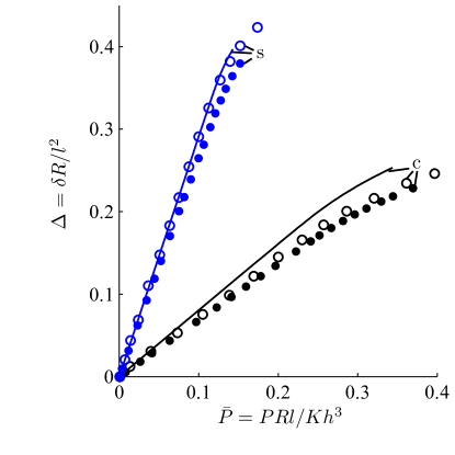
Figure 6: Non-adhesive contact of clamped (‘c’) and simply supported (‘s’) beams. The displacement $\Delta$ of the punch is shown as a function of the total load $\bar{P}$. See also the caption of Fig. 5.

Next, in Fig. 4 we compare our results for contact pressures $ap\left(\bar{x}\right)$ with those of Keer and Miller (1983) for both clamped and simply supported beams. We find an extremely close match between the two untill $a/h\approx 2$. Beyond that, while the match remains close for almost the entire contact area, a deviation is observed at the center of the contact patch: we find negative pressures at the center of the contact patch, whereas Keer and Miller (1983) report no negative contact pressure. From this, it appears that the earlier formulations of Keer and Miller (1983) – also Sankar and Sun (1983), which we discuss later – do not predict contact loss. Figure 4 confirms our previous observation that contact pressures of clamped and simply supported beams do not vary much, when scaled as $ap(\bar{x})/P$.

Next, in Fig. 5 we plot the variation of the contact area $A$ with the total load $\bar{P}$ on the punch and the punch’s displacement $\Delta$ for both clamped and simply supported beams. We also compare with FE computations and results of Sankar and Sun (1983). The process is repeated for the variation of $\Delta$ with $\bar{P}$ in Fig. 6. Figure 5(a) shows that for the same contact area $A$, the load $\bar{P}$ required for a simply supported beam is small compared to a clamped beam. This is because the simply supported beam bends more easily. This is also why we observe greater displacements $\Delta$ in these beams in Figs. 5(b) and 6. Finally, Figs. 5 and 6 show a close match of our theoretical predictions with FE computations and the results of Sankar and Sun (1983).

As in Paper 1, we now set the Young’s modulus and Poisson’s ratio to $E=0.083$ MPa and $\nu=0.4$, respectively, as representative of typical adhesives. We also use these material parameters while studying the adhesive beams. The geometric parameters remain unchanged, i.e. $l=40$ mm, $R=225$ mm, $h=4$ mm.

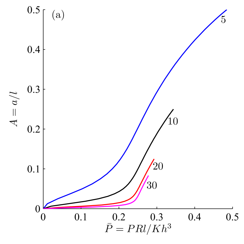
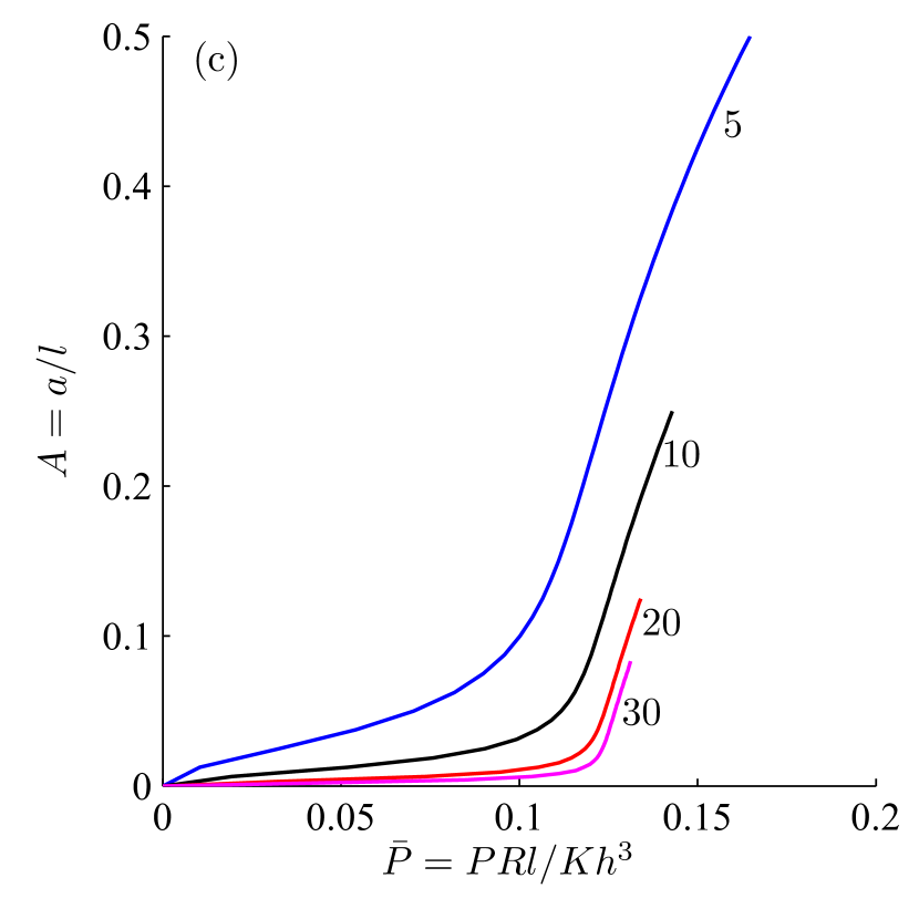
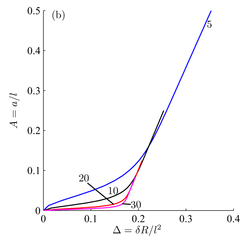
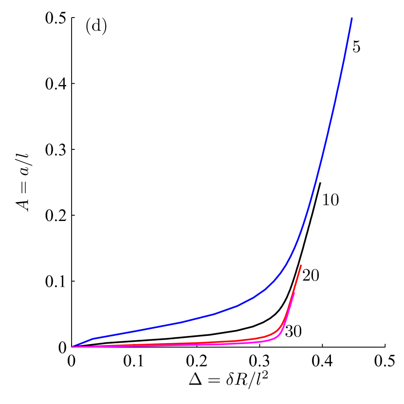
Figure 7: Non-adhesive contact of clamped (top row) and simply supported (bottom row) beams. Variation of contact area $A$ with total load $\bar{P}$ and punch’s displacement $\Delta$ is shown. Different slenderness ratios $l/h$ are considered and these are noted next to their associated curves.

In Fig. 7, we plot the variation of the contact area $A$ with respect to the total load $\bar{P}$ acting on the punch and the punch’s displacement $\Delta$ at several slenderness ratios $l/h$ for both clamped and simply supported beams. With increasing $l/h$ the beam’s resistance to bending decreases and, hence, we find smaller loads $\bar{P}$, or larger deflections $\Delta$, at the same contact area $A$. For the same reason the load $\bar{P}$ required to achieve the same $A$ in simply supported beam is smaller than the ones for clamped beams. At the same time, the displacements $\Delta$ are higher for simply supported beams.

In Fig. 7, we observe that the curves change their slope abruptly. This is due to the beam wrapping around the punch rapidly with only a small increase in the load or the punch’s displacement. However, the plots in Fig. 7 do not reflect this aspect well, as $l$ is a common parameter in $A$, $\bar{P}$, $\Delta$ and $l/h$. At the end of this section we will employ an alternative set of non-dimensional variables which will provide clearer insight.

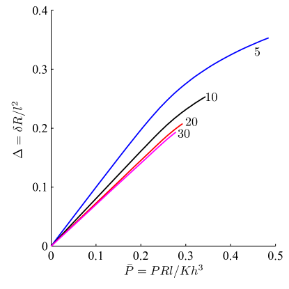
(a)

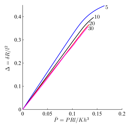
(b)

Figure 8: Non-adhesive contact of (a) clamped and (b) simply supported beams. Variation of punch’s displacement $\Delta$ with total load $\bar{P}$ is shown. Several slenderness ratios $l/h$, as noted next to their associated curves, are considered.

Next, in Fig. 8 we plot the variation of $\Delta$ with $\bar{P}$ for various $l/h$ for both clamped and simply supported beams. In Paper I, we found that these collapsed onto a single curve. This is not observed in Fig. 8. This collapse observed in Paper I was driven by the assumption that displacement at the bottom surface of the beam was given by the displacement of an Euler-Bernoulli beam. The relationship between $\Delta$ and $\bar{P}$ for Euler-Bernoulli beams with different $l/h$ is self-similar. However, here, the displacement of the bottom surface is found directly as a solution to the elasticity problem and is distinct from that obtained in Paper I.

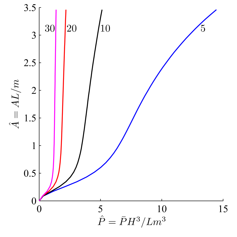
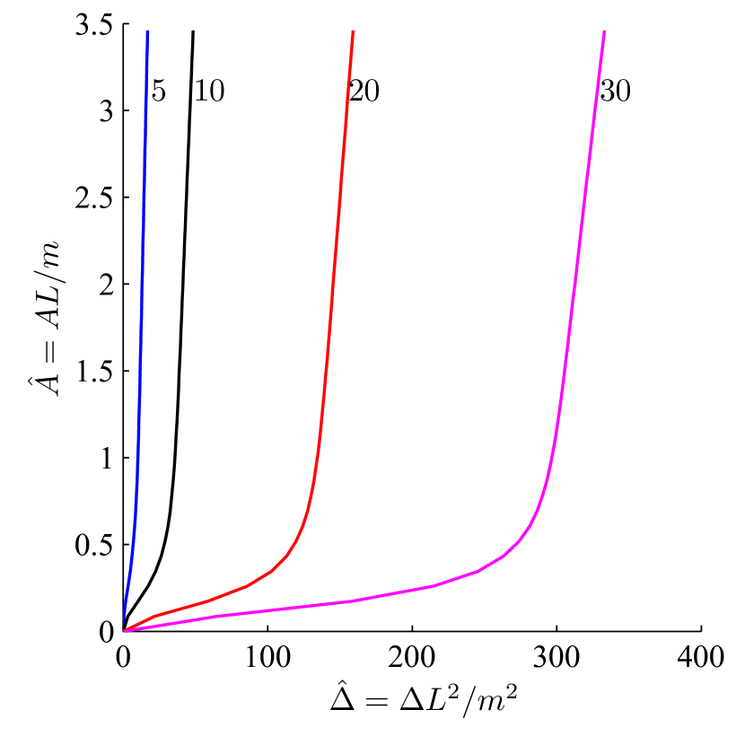
Figure 9: Non-adhesive contact of clamped beams. Variation of contact area $\hat{A}$ with (a) total load $\hat{P}$ and (b) punch’s displacement $\hat{\Delta}$ is shown. Different slenderness ratios $l/h$ are considered and these are noted next to their associated curves.

We return to explaing the sudden change of slope observed in the curves of Fig. 7. To this end, we follow Maugis (1992) and employ the non-dimensionalized parameters

$$\hat{A}=\frac{AL}{m}=a\left(\frac{K}{\pi wR^{2}}\right)^{1/3},\quad\hat{P}=\frac{\bar{P}H^{3}}{Lm^{3}}=\frac{P}{\pi w}\quad\text{ and}\quad\hat{\Delta}=\frac{\Delta L^{2}}{m^{2}}=\delta\left(\frac{K^{2}}{\pi^{2}w^{2}R}\right)^{1/3},$$ (7.4)

where $H=h/R$, instead of, respectively, $A$, $P$ and $\Delta$, to report our results. We set the adhesion energy $w=0.02\times 10^{-3}\text{ J}/\text{mm}^{2}$. In the present case of non-adhesive contact $w$ serves only to facilitate non-dimensionalization.

We plot the variation of $\hat{A}$ with $\hat{P}$ and $\hat{\Delta}$ at several $l/h$ in Fig. 9. Only clamped beams are considered. The results for simply supported beams are qualitatively similar. The rapid wrapping of the beam is reflected by the sudden increase in A in Fig. 9. As slender beams bend easily, this wrapping happens at lower loads for such beams; see Fig. 9(a). For the same reason, we observe more displacement in these beams in Fig. 9(b).

8 Results: Adhesive contact - JKR approximation

The JKR approximation is recovered when the scaled adhesive strength $\lambda\rightarrow\infty$ and the adhesive zone vanishes, i.e. $\bar{c}\rightarrow 1$. Hence, equations (3) and (3) become, respectively,

$$\Delta-\frac{1}{2}\,\bar{x}^{2}A^{2} =\frac{8\hat{\gamma}^{3}}{3\pi}\sum_{n=0}^{N}b_{2n}\mathcal{J}^{t}_{2n}\left(\bar{x}\right)+\frac{1}{\pi\hat{\gamma}}\sum_{n=1}^{M}d_{n}\mathcal{Q}^{t}_{n}\left(\bar{x}\right)$$ (8.1)

and $$0 =\frac{8\hat{\gamma}^{3}}{3\pi}\sum_{n=0}^{N}b_{2n}\mathcal{J}^{b}_{2n}\left(\hat{x}\right)+\frac{\hat{\gamma}}{\pi}\sum_{n=1}^{M}d_{n}\mathcal{Q}^{b}_{n}\left(\hat{x}\right).$$ (8.2)

The end condition on the contact pressure is determined by the Griffith criterion (3.12). By substituting (4.1) in (3.12), we obtain

$$b_{0}+b_{2}+\cdots+b_{2N}=-\frac{m}{2\pi L}\left(\frac{l}{h}\right)^{3}\frac{\sqrt{6Am}}{L}.$$ (8.3)

We now solve (8.1) – (8.3) through the algorithm of Sec. 5.

In Fig. 10 we plot the variation of the contact area $\hat{A}$ with the load $\hat{P}$ acting on the punch and the displacement $\hat{\Delta}$ of the punch for both clamped and simply supported beams. The slenderness ratio $l/h$ is kept constant, but two different combinations of $l$ and $h$ are investigated. We observe that the curves for same $l/h$ are sensitive to $l$ and $h$ individually and depend not only on the slenderness ratio. This was also observed in Paper I. This may be traced back to the presence of $L=l/R$ on the right hand side of (8.3). It is easier to explore the dependence of $h$ and $l$ repeatedly by employing $\hat{A}$, $\hat{P}$ and $\hat{\Delta}$ and we do so in Figs. 11 and 12.

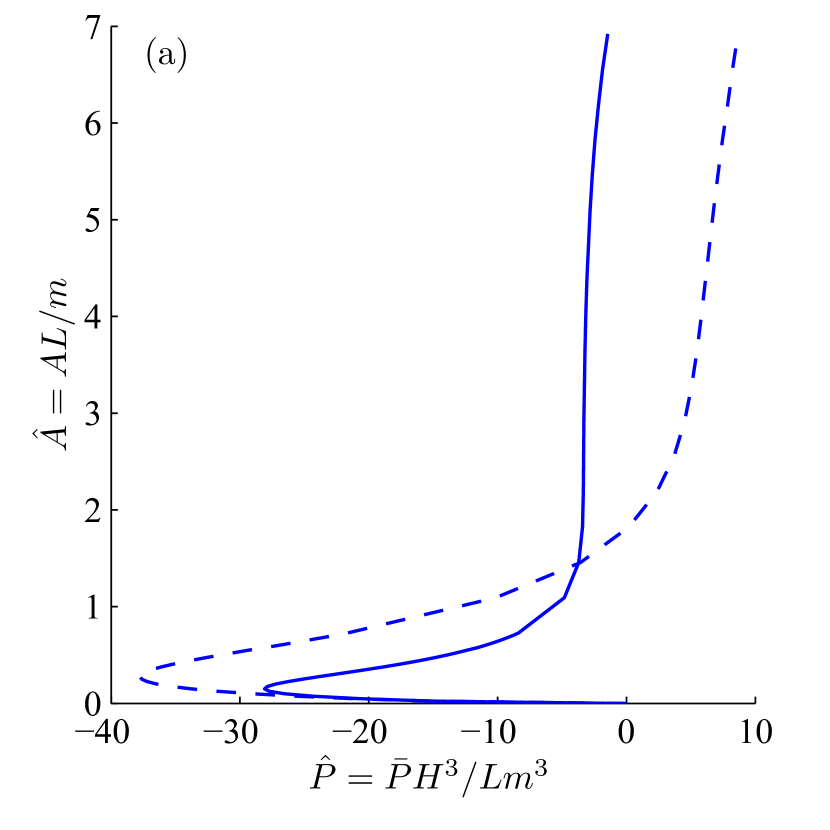
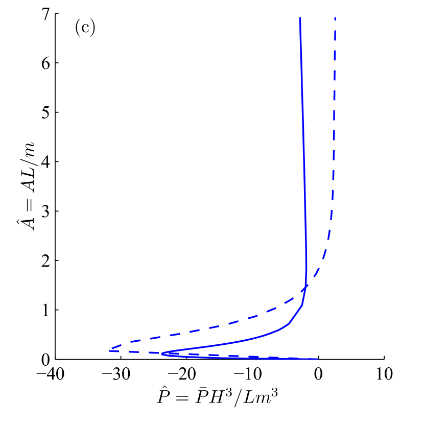
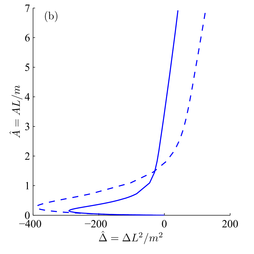
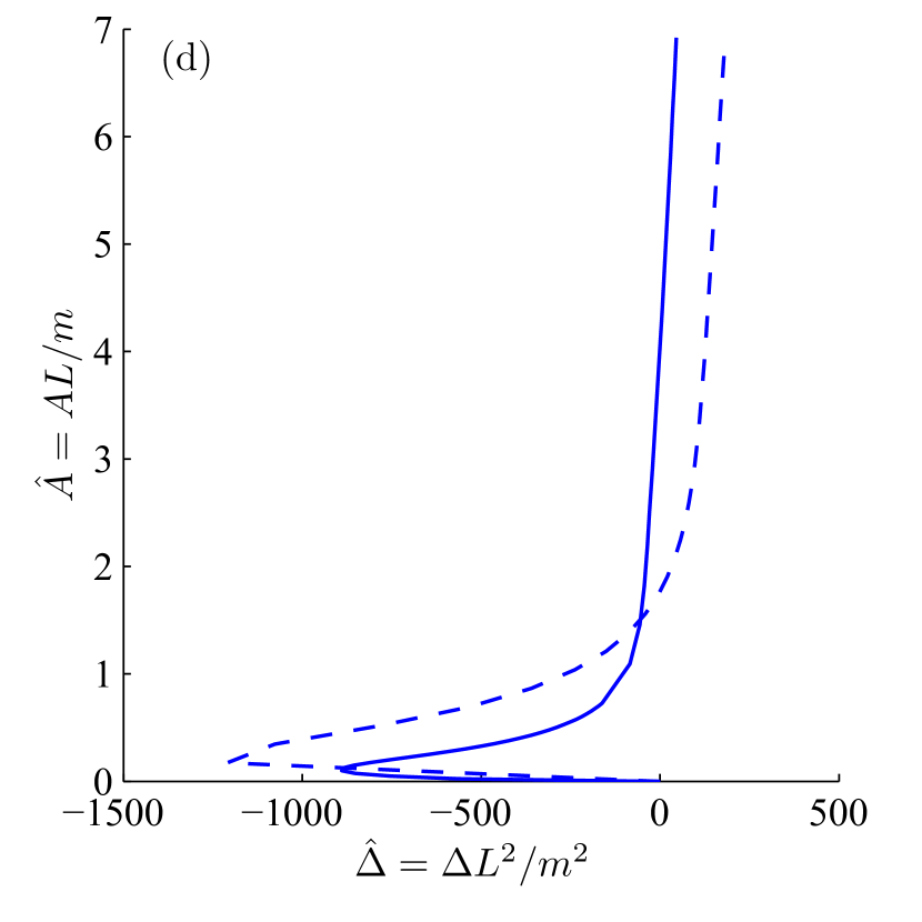
Figure 10: Adhesive contact of clamped (top row) and simply supported (bottom row) beams with the JKR approximation. Variation of contact area $\hat{A}$ with the total load $\hat{P}$ are shown in (a) and (c), and the punch’s displacement $\hat{\Delta}$ are shown in (b) and (d). The beam’s slenderness ratio $l/h=10$. Solid lines correspond to $l=40$ mm and $h=4$ mm, while the dashed line is for a beam with $l=80$ mm and $h=8$ mm.

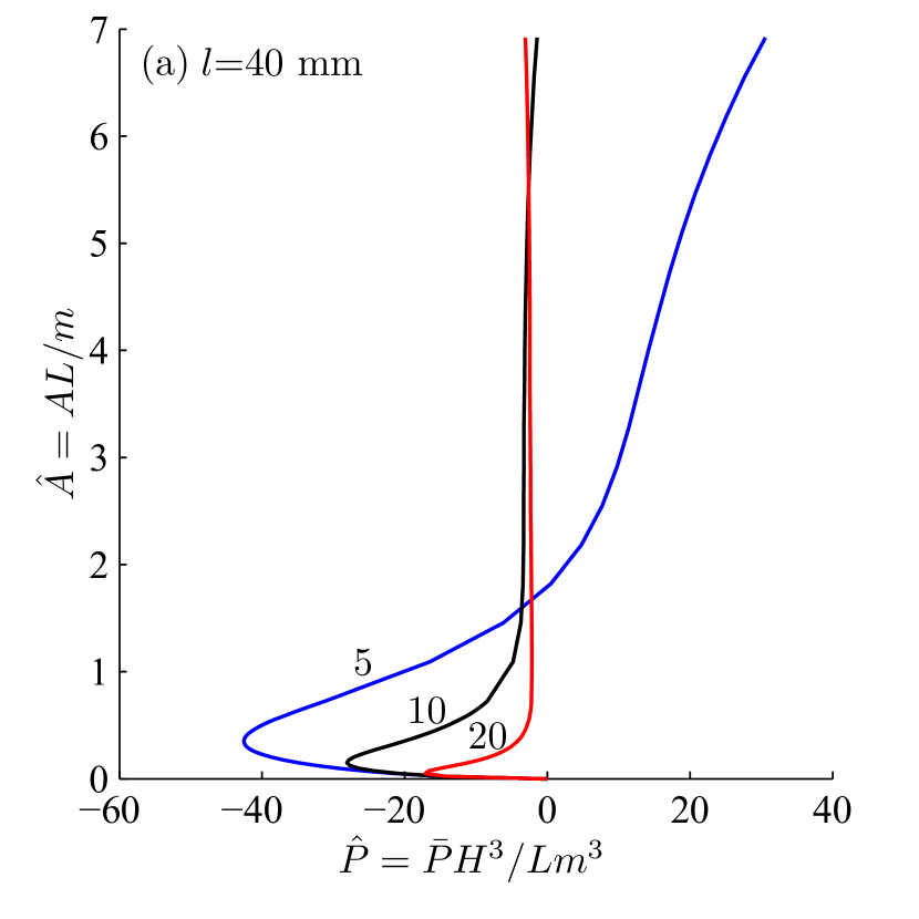
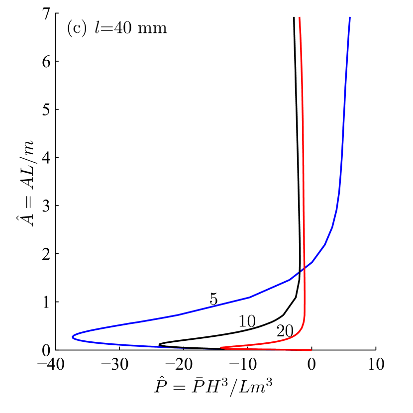
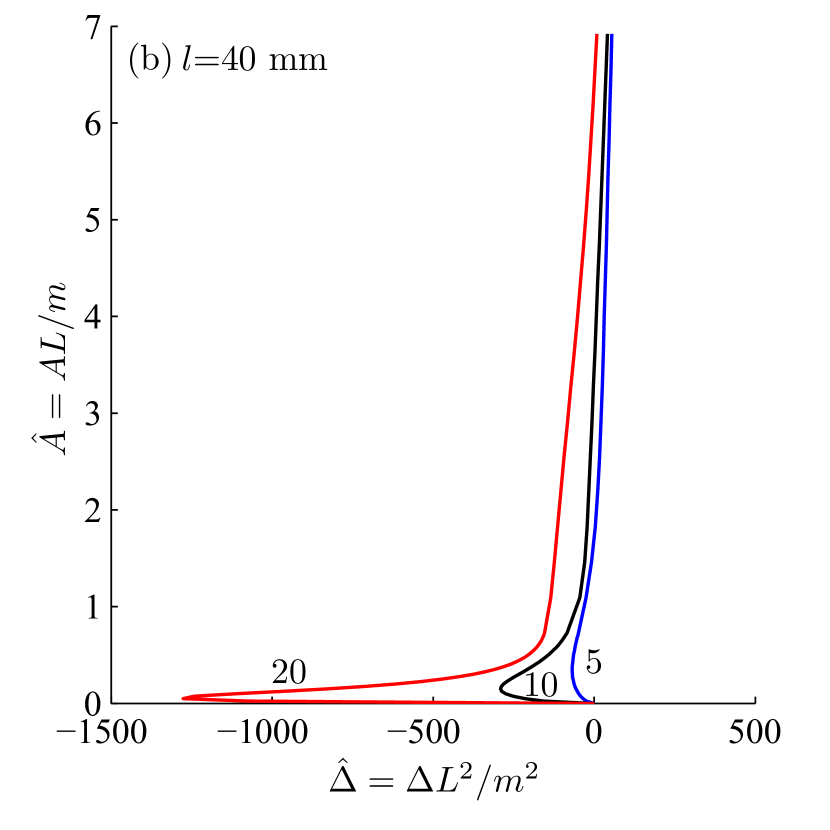
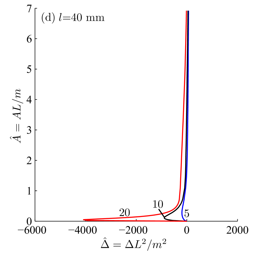
Figure 11: Adhesive contact of clamped (top row) and simply supported (bottom row) beams with the JKR approximation. Left column, i.e. (a) and (c), reports the variation of contact area $\hat{A}$ with total load $\hat{P}$, while the right column, i.e. (b) and (d), plots the change of $\hat{A}$ with the punch’s displacement $\hat{\Delta}$. Results are obtained for several slenderness ratios $l/h$ as noted next to their curves, while keeping $l=40$ mm.

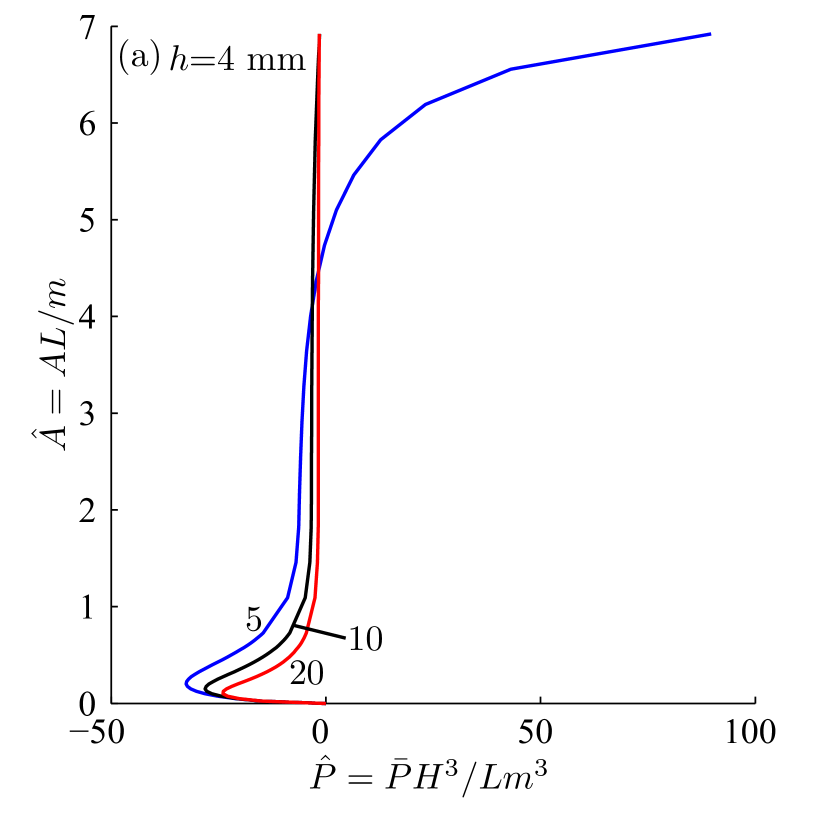
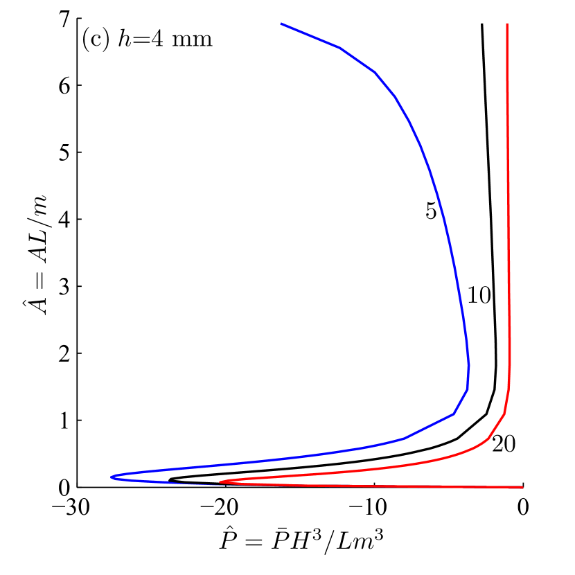
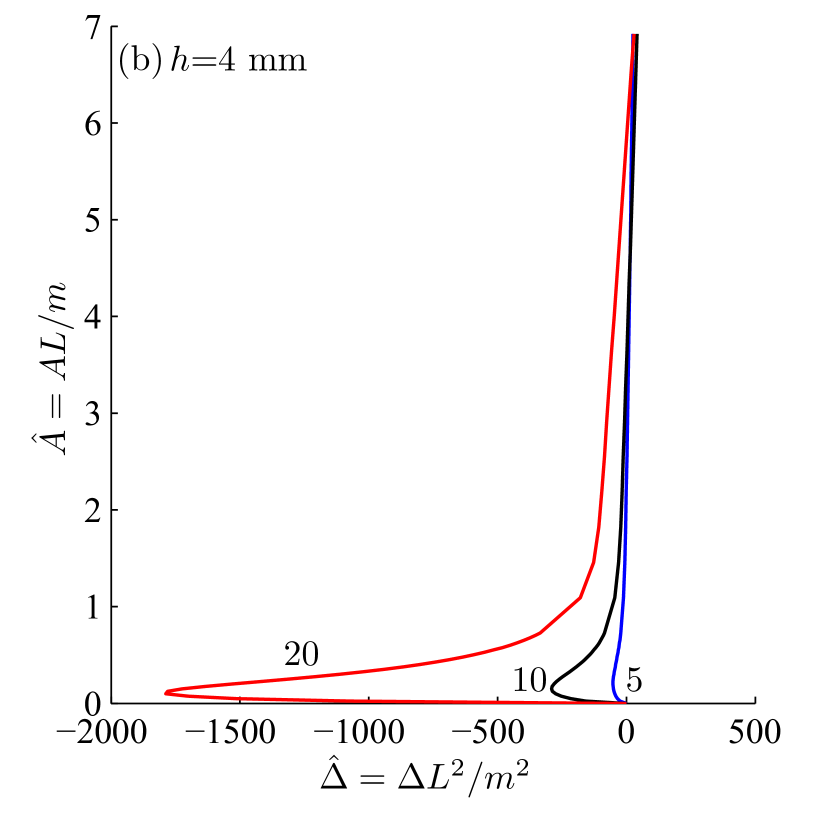
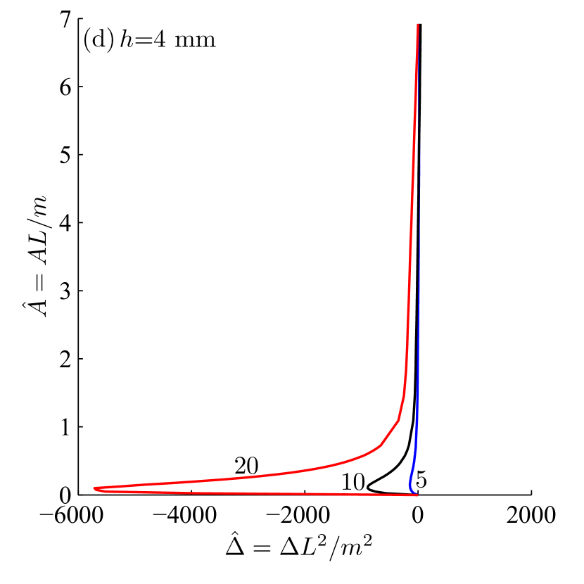
Figure 12: Adhesive contact of clamped (top row) and simply supported beams (bottom row) with the JKR approximation. Left column, i.e. (a) and (c), reports the variation of contact area $\hat{A}$ with total load $\hat{P}$, while the right column, i.e. (a) and (c), plots the change of $\hat{A}$ with the punch’s displacement $\hat{\Delta}$. Results are obtained for several slenderness ratios $l/h$ as noted next to their curves, while keeping $h=4$ mm.

Curves in Fig. 11 are obtained for several $l/h$ by varying $h$ while keeping $l=40$ mm. Beams with high $l/h$ ratio bend easily due to the adhesion, and we observe smaller negative loads $\hat{P}$ and larger negative displacements $\hat{\Delta}$ at a given contact area $\hat{A}$. Note that negative loads and displacements indicate, respectively, tensile force on the punch and the upward bending of beams. From Fig. 11 we observe that these slender beams wrap around – as indicated by sudden slope changes in $\hat{A}$ versus $\hat{P}$ and $\hat{\Delta}$ curves – the punch earlier, i.e. at smaller $\hat{P}$. For sufficiently slender beams, the wrapping occurs even when there is no compressive (positive) load on the punch. In these beams the bending resistance is unable to counterbalance adhesive forces. The above features, viz. extent of wrapping and the response to adhesive forces, are, expectedly, heightened in the case of simply supported beams, whose bending resistance is lower.

Finally, we plot the variation of the contact area $\hat{A}$ with the load $\hat{P}$ acting on the punch and the displacement $\hat{\Delta}$ for several slenderness ratios $l/h$. We change $l$ and set $h=4$ mm. The results for both clamped and simply supported beams are shown in Fig. 12. Qualitatively Fig. 12 is similar in many respects to Fig. 11. From Fig. 12(c), we observe that, for $\hat{A}\gtrsim 1.5$ in a simply supported beam of $l/h=5$, the load $\hat{P}$ decreases with the increase in contact area $\hat{A}$. At the same time, the punch’s displacement $\hat{\Delta}$ increases; see Fig. 12(d). This is explained by the presence of negative (tensile) stresses at the center of the contact area in addition to the very large negative stresses allowed in the contact pressure distribution at the contact edges. The contact area over which these tensile stresses act also increases with the increase in contact area. Hence, the load $\hat{P}$ decreases with the increase in contact area $\hat{A}$.

9 Results: Adhesive contact with an adhesive zone model

Finally, we study the behaviour of adhesive beams indented by a rigid cylindrical punch with the help of adhesive-zone models. In these models an adhesive force acts over an adhesive zone of length $d=c-a$ outside the contact area. Here, we model the distribution of the adhesive forces through the Dugdale-Barenblatt model, so that the normal traction on the (extended) beam’s top surface is given by (2.9). The contact problem is resolved by solving (4.6) – (4.9) following the solution procedure of Sec. 5.

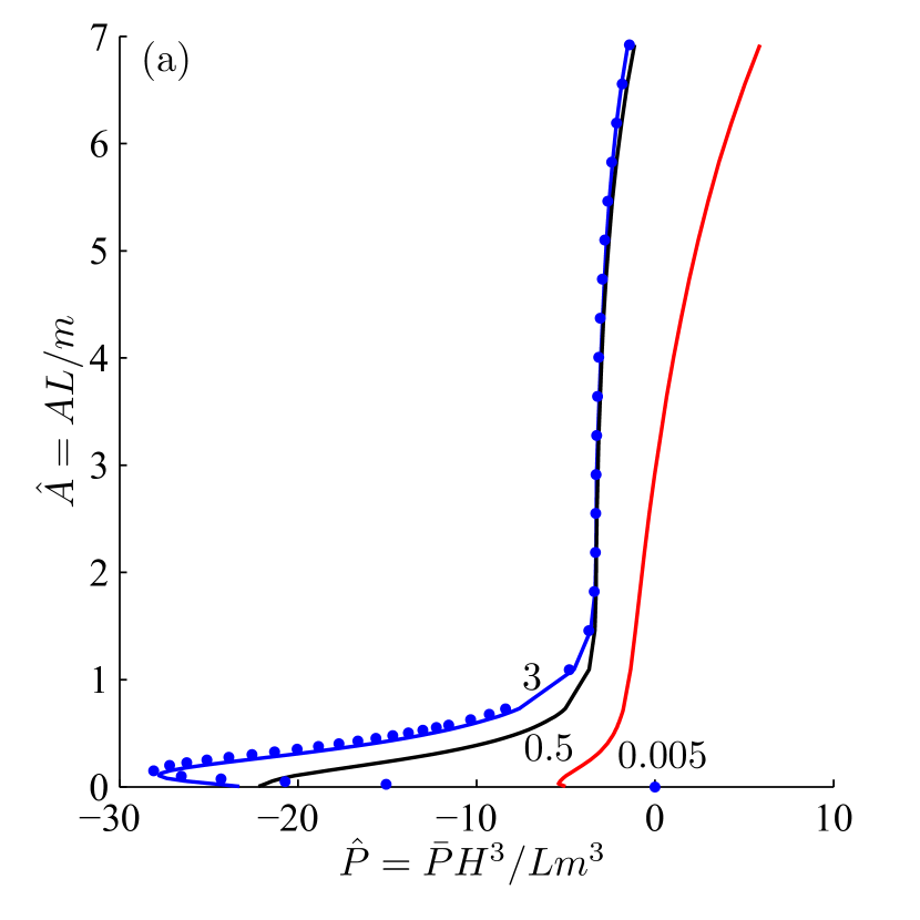
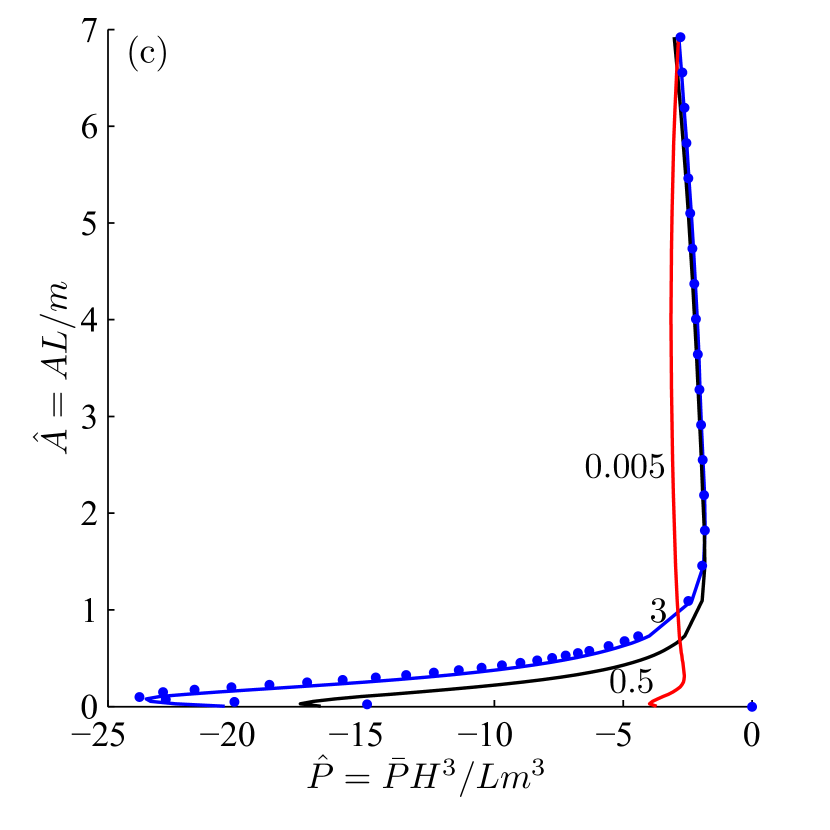
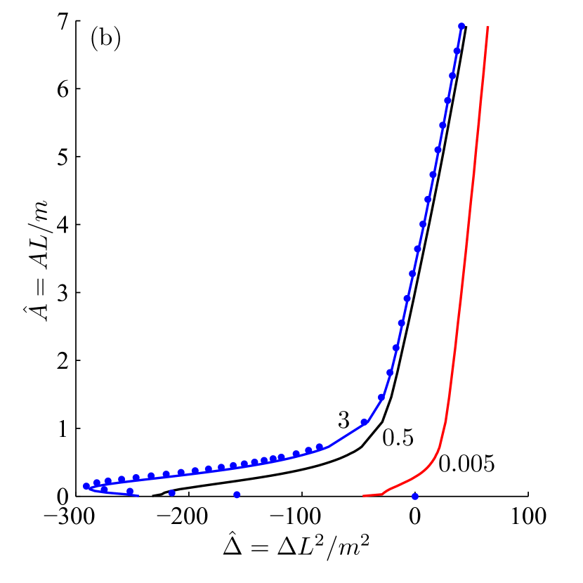
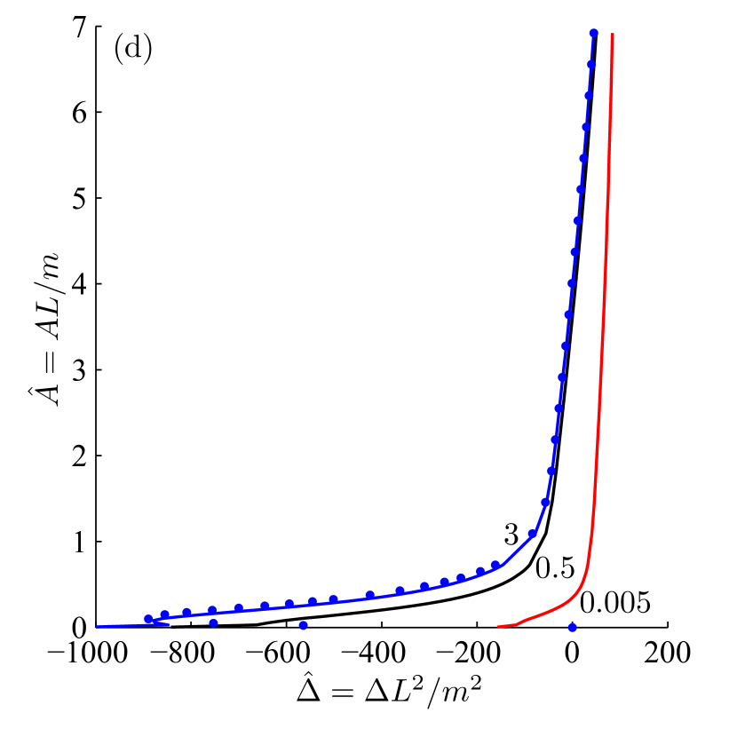
Figure 13: Adhesive contact of clamped (top row) and simply supported (bottom row) beams with an adhesive zone model. Variation of contact area $\hat{A}$ with the total load $\hat{P}$ are shown in (a) and (c), and the punch’s displacement $\hat{\Delta}$ are shown in (b) and (d). Different adhesive strengths $\lambda$ are considered and these are indicated next to their associated curves. The beam’s thickness $h=4$ mm and $l=40$ mm. Filled circles represent the JKR solution for the corresponding beam; cf. Sec. 8

For brevity, we report here the effect of only the adhesive strength $\lambda$ at a given $l$ and $h$, as the response to varying $l/h$ is found to be the same as in Sec. 8.

In Fig. 13 we plot the variation of the contact area $\hat{A}$ with the total load $\hat{P}$ and the displacement $\hat{\Delta}$ for several adhesive strengths $\lambda$. We observe that as $\lambda\rightarrow 0$ the results approach those obtained for non-adhesive interaction as in Sec. 7. At the same time, increasing adhesive strength pushes our results towards those obtained for the JKR approximation in Sec. 8.

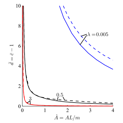
Figure 14: Variation of the adhesive zone size $\bar{d}$ with the the contact area $\hat{A}$ at different adhesive strengths $\lambda$ for a clamped beam. We set l=$40$ mm and $h=4$ mm. Solid lines indicate the predictions of the formulation mentioned in this article, while the dotted lines are those obtained from the formulation of the Paper I.

Next, we study the effect of adhesive strength $\lambda$ on the adhesive zone size $\bar{d}=\bar{c}-1$. For this, we plot $\bar{d}$ by varying $\hat{A}$ for several adhesive strengths in Fig. 14. From Fig. 14, we observe that with increasing $\lambda$, $\bar{d}$ goes to zero. We also find that, due to the difference in formulations, the results obtained in this article are quite different from those of Paper 1 at low to moderate adhesive strengths. At high $\lambda$ there is not much difference between the two. Finally, as seen in Paper I, varying the slenderness ratio $l/h$ and constraints imposed by end supports do not effect the adhesive zone size much.

10 Comparisons with Paper I

We now compare predictions of the formulation of this paper with Paper I for both non-adhesive and adhesive contacts. For this, we plot the variation of the contact area $\hat{A}$ with variation in the total load $\hat{P}$ acting on the punch for clamped and simply supported beams as shown in Fig. 15. For the non-adhesive beams, we also plot FE results to show the comparison better; see Fig. 15(a). From Fig. 15(a), we observe that both the semi-analytical formulations predicts the behavior of the beams correctly for small $\hat{A}$. However, with increasing $\hat{A}$, predictions of the current formulation are closer to the FE simulations than those of Paper I. Finally, from Fig. 15(b), we observe that both the formulations predicts the same behavior in the beams before wrapping in the JKR approximation of the contact. However, for a large portion of the contact area the results of both the formulations predicts the behaviour of the beams differently. Thus, to establish the correctness of these formulations, we need to study the behaviour of the beams experimentally. So, in the next section, we check the experimental feasibility for the indentation in adhesive beams.

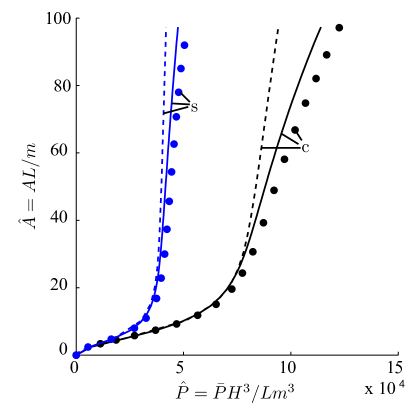
(a)

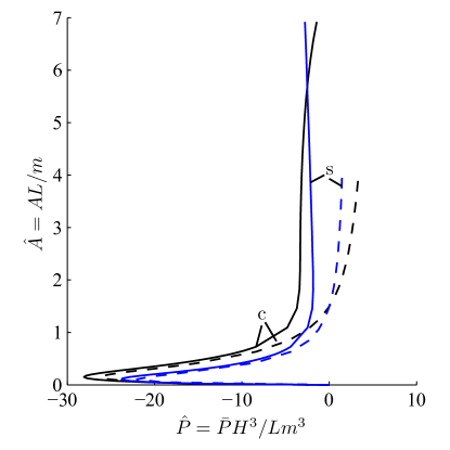
(b)

Figure 15: The contact area $A$ is plotted as a function of the total load $\bar{P}$ acting on the punch. (a) Non-adhesive contact of clamped (‘c’) and simply supported (‘s’) beams. The beam’s slenderness ratio $l/h$=10. We set $E=2000$ MPa and $\nu=0.3$. (b) Adhesive contact of clamped (‘c’) and simply supported (‘s’) beams with JKR approximation. We set $h=4$ mm, $l=40$ mm, $E=0.083$ MPa and $\nu=0.4$. Solid lines are results obtained from the semi-analytical procedure of Sec. 4, while the dashed line are results from Paper I. Filled circles correspond to FE simulations of Sec. 6.

11 Experimental validation feasibility for the adhesive contact

In this section, we see the feasibility of conducting the JKR experiments for the beams with our experimental set-up mentioned in Paper I. For this purpose, we first obtain predictions for PDMS (poly-dimethyl- siloxane) samples employed in Paper I utilizing the formulations of this paper and Paper I. The PDMS samples were prepared using a 10:1 weight ratio mixture of Sylgard 184 silicone elastomer base and curing agent. We consider clamped beams with fixed half-span $l=50$ mm and vary the thickness $h$ between $1$ mm and $25$ mm. The results are shown in Fig. 16.

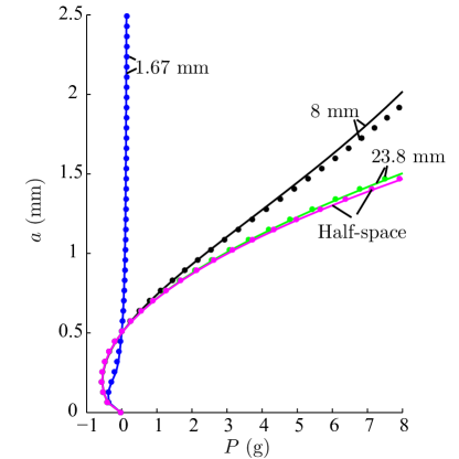
Figure 16: Variation of the contact area a (in mm) with the total load P (in g) for adhesive clamped beams with half-span l = 50 mm at several thicknesses $h$, as noted next to their curves. We set $E=1.237$ MPa, $W=27.941$ N/mm. The contact is modeled by the JKR approximation of the contact. Solid lines correspond to theoretical predictions of Paper I, while the asterisk represent those of current approach.

In our experiments, the maximum value of the load $P$ is limited by our micro-weighing balance. From Fig. 16, we observe that with a 10:1 PDMS material, we can not clearly distinguish the results obtained by the formulation of this paper and that of Paper I. The limitations of the load measuring capability of our micro-weighing balance used in the experimental set-up makes differentiating between the predictions of our current and previous (Paper I) formulations hard. To achieve this with our current experimental set-up requires a softer material with strong adhesive characteristics than PDMS.

12 Conclusions

The assumption made in the Paper I about the vertical displacement of the beam’s bottom surface limits the range of the corresponding semi-analytical analysis. In this paper we removed this constraint by solving for the vertical displacement directly, thereby extended the applicability of the formulation. The current formulation modeled the indention of adhesive beam in terms of two coupled Fredholm integral equations of first kind. These dual integral equations were solved through a collocation technique employing series approximations for the unknown contact pressure and bottom surface’s vertical displacement. Care should be exercised when selecting the approximating series for the displacement. We then compared our predictions with FE simulations and previously published results for non-adhesive indentation, and found a satisfactory match for a wide range of indentation. Next, we presented the results for JKR approximation and adhesive zone model approximation of the contacts. Finally, we studied the experimental feasibility to establish the varacity of the current approach. However, for this we need a softer adhesive material than the PDMS – which we are in search of.

In the future we aim to extend the present approach to three-dimensional axi-symmetric indentation. More immediately though, in part III of this work, we will present experimental data for the adhesive indentation of beams.

Appendix A Vertical displacement of the beam’s top surface ($V\left(\xi,0\right)$) and normal traction at its bottom surface ($S_{yy}\left(\xi,h\right)$) in Fourier space

In Fourier space the transformed horizontal and vertical displacements may be solved as, respectively,

$$U\left(\xi,y\right) =\left(\kappa a_{1}+\xi y\left(a_{1}+ia_{3}\right)\right)e^{\xi y}+\left(\kappa b_{1}-\xi y\left(b_{1}-ib_{3}\right)\right)e^{-\xi y},$$ (A.1)

$$\text{and }\quad V\left(\xi,y\right) =\left(\kappa a_{3}+i\xi y\left(a_{1}+ia_{3}\right)\right)e^{\xi y}+\left(\kappa b_{3}+i\xi y\left(b_{1}-ib_{3}\right)\right)e^{-\xi y},$$ (A.2)

with

$$U\left(\xi,y\right)=\int\limits_{-\infty}^{\infty}u\left(x,y\right)e^{i\xi x}dx,\quad V\left(\xi,y\right)=\int\limits_{-\infty}^{\infty}v\left(x,y\right)e^{i\xi x}dx,$$

and unknown constants $a_{1}$, $a_{3}$, $b_{1}$, and $b_{3}$. These constants are obtained by applying the boundary conditions, which in Fourier space are

$$\text{at}\;\;y=0: \quad S_{\xi y} =0, \quad S_{yy} =\bar{P}(\xi),$$ (A.3a)

$$\text{at}\;\;y=h: \quad S_{\xi y} =0, \quad V =\bar{v}(\xi),$$ (A.3b)

with

$$S_{\xi y} = \frac{E}{2\left(1+\nu\right)}\left(\frac{d}{dy}U-i\xi V\right),$$

$$S_{yy} = \frac{E}{\left(1+\nu\right)}\left(\frac{d}{dy}V+\frac{\nu}{1-2\nu}\left(-i\xi U+\frac{d}{dy}V\right)\right),$$

$$\bar{P}(\xi) = \int\limits_{-\infty}^{\infty}-P\left(x\right)e^{i\xi x}dx\quad\text{and }\quad\bar{v}(\xi)=\int\limits_{-\infty}^{\infty}v\left(x\right)e^{i\xi x}dx.$$

With this, we find the vertical displacement of the top surface in Fourier space to be

$$V\left(\xi,0\right)= -\frac{2\,\bar{P}\left(\xi\right)}{E^{*}}\,\frac{\sinh^{2}{\xi\,h}}{\xi\left(\xi\,h+\sinh{\xi\,h}\cosh{\xi\,h}\right)}+\bar{v}\left(\xi\right)\,\frac{\sinh{\xi\,h}+\xi\,h\cosh{\xi\,h}}{\xi\,h+\sinh{\xi\,h}\cosh{\xi\,h}},$$

and the normal traction at the bottom layer in Fourier space to be

$$S_{yy}\left(\xi,h\right) =\bar{P}\left(\xi\right)\,\frac{\sinh{\xi\,h}+\xi\,h\cosh{\xi\,h}}{\xi\,h+\sinh{\xi\,h}\cosh{\xi\,h}}+E^{*}\bar{v}\left(\xi\right)\,\frac{\xi}{2}\,\frac{\sinh^{2}{\xi\,h}-\xi^{2}\,h^{2}}{\xi\,h+\sinh{\xi\,h}\cosh{\xi\,h}},$$

where $E^{*}={E}/{\left(1-\nu^{2}\right)}$.

Appendix B Displacement calculations

B.1 Clamped beam

We approximate the vertical displacement of the bottom surface in a beam that is clamped at the ends as

$$\vartheta^{c}_{b}\left(\hat{\tau}\right)=d^{c}_{0}+\sum_{n=1}^{M}d^{c}_{n}\cos\left(n\pi\hat{\tau}\right).$$ (B.1)

The above displacement filed is symmetric in $\hat{\tau}$, i.e., $\vartheta^{c}_{b}\left(\hat{\tau}\right)=\vartheta^{c}_{b}\left(-\hat{\tau}\right)$. The slope conditions at the ends, i.e., $d\vartheta^{c}_{b}/d\hat{\tau}=0$ at $\hat{\tau}=\pm 1$, are automatically satisfied. We find the unknown coefficient $d^{c}_{0}$ in the displacement employing $\vartheta^{c}_{b}\left(\pm 1\right)=0$, to obtain

$$d^{c}_{0}=\sum_{n=1}^{M}d^{c}_{n}\left(-1\right)^{n+1}.$$ (B.2)

Combining (B.1) and (B.2) yields

$$\vartheta^{c}_{b}\left(\hat{\tau}\right)=\sum_{n=1}^{M}d^{c}_{n}\left[\left(-1\right)^{n+1}+\cos\left(n\pi\hat{\tau}\right)\right].$$ (B.3)

Differentiating the above twice with respect to $\hat{\tau}$ provides

$$\kappa^{c}_{b}\left(\hat{\tau}\right)=-\pi^{2}\sum_{n=1}^{M}d^{c}_{n}n^{2}\cos\left(n\pi\hat{\tau}\right).$$ (B.4)

B.2 Simply supported beam

For a simply supported beam, we approximate the vertical displacement of the elastic layer’s bottom surface in $-1\leq\hat{\tau}\leq 1$, which should be symmetric in $\hat{\tau}$, as

$$\vartheta^{s}_{b}\left(\hat{\tau}\right)=d^{s}_{0}+\sum_{n=1}^{M}d^{s}_{2n-1}\sin\left\{\frac{\left(2n-1\right)\pi\left(\hat{\tau}+1\right)}{2}\right\}.$$ (B.5)

The above displacement field also satisfies $d^{2}\vartheta^{s}/d\hat{\tau}^{2}=0$ at $\hat{\tau}=\pm 1$, as appropriate for a simply supported beam. Satisfying $\vartheta^{s}\left(\pm 1\right)=0$, makes the unknown constant $d^{s}_{0}=0$. Hence, $\vartheta_{b}^{s}\left(\hat{\tau}\right)$ becomes

$$\vartheta^{s}_{b}\left(\hat{\tau}\right)=\sum_{n=1}^{M}d^{s}_{2n-1}\left(-1\right)^{n-1}\cos\left\{\frac{\left(2n-1\right)\pi\hat{\tau}}{2}\right\}.$$ (B.6)

Differentiating the above twice we obtain the curvature $\kappa^{s}_{b}\left(\hat{\tau}\right)$ in $-1\leq\hat{\tau}\leq 1$ as

$$\kappa^{s}_{b}\left(\hat{\tau}\right) = -\sum_{n=1}^{M}d^{s}_{2n-1}\left(-1\right)^{n-1}\left(\frac{\left(2n-1\right)\pi}{2}\right)^{2}\cos\left(\frac{\left(2n-1\right)\pi\hat{\tau}}{2}\right).$$ (B.7)

Calculating the slope at the ends of the beam yields

$$\left.\frac{d\vartheta^{s}_{b}\left(\hat{\tau}\right)}{d\hat{\tau}}\right|_{\hat{\tau}=1}=-\sum_{n=1}^{M}d^{s}_{2n-1}\frac{\left(2n-1\right)\pi}{2}.$$ (B.8)

Finally, finding the displacement in $1<\hat{\tau}<\infty$, by extending the beam along its slope at the end supports, we obtain

$$\vartheta^{s}_{b}\left(\hat{\tau}\right)=\left.\frac{d\vartheta^{s}\left(\hat{\tau}\right)}{d\hat{\tau}}\right|_{\hat{\tau}=1}\left(\hat{\tau}-1\right).$$ (B.9)

Appendix C Calculating $\bar{\vartheta}_{b}\left(\hat{\omega}\right)$ and $\bar{\kappa}_{b}\left(\hat{\omega}\right)$

As in Paper I, here too we consider the beams as linear elastic layers of infinite length. Thus, we employ mollifiers to find $\hat{\vartheta}_{b}\left(\hat{\omega}\right)$ and $\hat{\kappa}_{b}\left(\hat{\omega}\right)$. Therefore, we write

$$\hat{\vartheta}_{b}\left(\hat{\omega}\right) =\int\limits_{-\infty}^{\infty}\vartheta_{b}\left(\hat{\tau}\right)W\left(\hat{\tau}\right)\cos{\hat{\omega}\hat{\tau}}\,d\hat{\tau}$$ (C.1)

and $$\hat{\kappa}_{b}\left(\hat{\omega}\right) =\int\limits_{-\infty}^{\infty}\frac{d^{2}}{d\hat{\tau}^{2}}\left[\vartheta_{b}\left(\hat{\tau}\right)W\left(\hat{\tau}\right)\right]\cos{\hat{\omega}\hat{\tau}}\,d\hat{\tau},$$ (C.2)

where the mollifier (Muthukumar, 2016)

$$W\left(\hat{\tau}\right) =\left\{\begin{array}[]{ll}1&\text{for }\left|\hat{\tau}\right|\leq\left|\hat{l}_{1}\right|,\\ w_{2}\left(\hat{\tau}\right)&\text{for }\left|\hat{l}_{1}\right|<\left|\hat{\tau}\right|<\left|\hat{l}_{2}\right|\\ 0&\text{for }\left|\hat{\tau}\right|\geq\left|\hat{l}_{2}\right|,\end{array},\right.$$ (C.3d)

and $$w_{2}\left(\hat{\tau}\right) =\frac{\exp\left\{{-1/\left(\hat{l}_{2}-\hat{\tau}\right)^{2}}\right\}}{\exp\left\{{-1/\left(\hat{l}_{2}-\hat{\tau}\right)^{2}}\right\}+\exp\left\{{-1/\left(\hat{\tau}-\hat{l}_{1}\right)^{2}}\right\}},$$ (C.3e)

with $\hat{l}_{1}$ and $\hat{l}_{2}$ locating portions of the beam that are far away from the ends with $\hat{l}_{2}>\hat{l}_{1}>>1$. The mollifier $W\left(\hat{\tau}\right)$ is infinitely differentiable, and alters the displacement far from the beam’s ends and makes it integrable.

C.1 Clamped beam

For a clamped beam, finding $\bar{\vartheta}^{c}_{b}\left(\hat{\omega}\right)$ and $\bar{\kappa}^{c}_{b}\left(\hat{\omega}\right)$, we obtain

$$\hat{\vartheta}^{c}_{b}\left(\hat{\omega}\right)=\sum_{n=1}^{M}d^{c}_{n}\hat{\beta}^{c}_{n}\left(\hat{\omega}\right)\quad\text{and}\quad\hat{\kappa}^{c}_{b}\left(\hat{\omega}\right)=\sum_{n=1}^{M}d^{c}_{n}\hat{\kappa}^{c}_{n}\left(\hat{\omega}\right),$$ (C.4)

where

$$\hat{\beta}^{c}_{n}\left(\hat{\omega}\right)=\frac{2\left(-1\right)^{n+1}\sin{\hat{\omega}}}{\hat{\omega}}+\frac{2\hat{\omega}\left(-1\right)^{n+1}\sin{\hat{\omega}}}{n^{2}\pi^{2}-\hat{\omega}^{2}}\quad\text{and}\quad\hat{\kappa}^{c}_{n}\left(\hat{\omega}\right)=-n^{2}\pi^{2}\,\frac{2\hat{\omega}\left(-1\right)^{n+1}\sin{\hat{\omega}}}{n^{2}\pi^{2}-\hat{\omega}^{2}}.$$

C.2 Simply supported beam

Evaluating $\bar{\vartheta}^{s}_{b}\left(\hat{\omega}\right)$ and $\hat{\kappa}{s}_{b}\left(\hat{\omega}\right)$ for a simply supported beam yields

$$\hat{\vartheta}^{s}_{b}\left(\hat{\omega}\right)=\sum_{n=1}^{M}\tilde{d}^{s}_{n}\,\hat{\beta}^{s}_{n}\left(\hat{\omega}\right)\quad\text{and}\quad\hat{\kappa}^{s}_{b}\left(\hat{\omega}\right)=\sum_{n=1}^{M}\tilde{d}^{s}_{n}\hat{\kappa}^{s}_{n}\left(\hat{\omega}\right),$$ (C.5)

where $\tilde{d}^{s}_{n}=d^{s}_{2n-1}$,

$$\hat{\beta}^{s}_{n}\left(\hat{\omega}\right)= \int\limits_{-1}^{1}\left(-1\right)^{n-1}\cos\left(\frac{\left(2n-1\right)\pi\hat{\tau}}{2}\right)\,\cos{\hat{\omega}\hat{\tau}}\,d\hat{\tau}-\left(2n-1\right)\pi\int\limits_{1}^{\hat{l}_{2}}\left(\hat{\tau}-1\right)\,W\left(\hat{\tau}\right)\,\cos{\hat{\omega}\hat{\tau}}\,d\hat{\tau}$$

and $$\hat{\kappa}^{s}_{n}\left(\hat{\omega}\right)= -\left(\frac{\left(2n-1\right)\pi}{2}\right)^{2}\,\int\limits_{-1}^{1}\left(-1\right)^{n-1}\cos\left(\frac{\left(2n-1\right)\pi\hat{\tau}}{2}\right)\,\cos{\hat{\omega}\hat{\tau}}\,d\hat{\tau}$$

$$-2\left(2n-1\right)\pi\int\limits_{\hat{l}_{1}}^{\hat{l}_{2}}\frac{dw_{2}\left(\hat{\tau}\right)}{d\hat{\tau}}\cos{\hat{\omega}\hat{\tau}}\,d\hat{\tau}-\left(2n-1\right)\pi\int\limits_{\hat{l}_{1}}^{\hat{l}_{2}}\left(\hat{\tau}-1\right)\frac{d^{2}w_{2}\left(\hat{\tau}\right)}{d\hat{\tau}^{2}}\,\cos{\hat{\omega}\hat{\tau}}\,d\hat{\tau}.$$

Finally, employing (C.4) and (C.5), we may write $\bar{\vartheta}_{b}\left(\hat{\omega}\right)$ and $\hat{\kappa}_{b}\left(\hat{\omega}\right)$, respectively, as

$$\hat{\vartheta}_{b}\left(\hat{\omega}\right)=\sum_{n=1}^{M}d_{n}\hat{\beta}_{n}\left(\hat{\omega}\right)\quad\text{and}\quad\bar{\kappa}_{b}\left(\hat{\omega}\right)=\sum_{n=1}^{M}d_{n}\hat{\kappa}_{n}\left(\hat{\omega}\right).$$ (C.6)

References

• Alexandrov and Pozharskii (2001) Alexandrov, A., Pozharskii, D. (2001). Three-dimensional contact problems. Kluwer Academic Publishers, Dordrecht, The Netherlands.
• Arul and Ghatak (2008) Arul, E. P., Ghatak, A. (2008). Bioinspired design of a hierarchically structured adhesive. Langmuir, 25: 611–617.
• (3) Barthel, E., Perriot, A. (2007). Adhesive contact to a coated elastic substrate. J. Phys. D: Appl. Phys., 40: 1059–1067.
• Chatterjee (2002) Chatterjee, A. (2002). Lecture notes: An elementary continuation technique. http://home.iitk.ac.in/~anindya/continuation.pdf.
• Chaudhury et al. (1996) Chaudhury, M. K., Weaver, T., Hui, C., Kramer, E. (1996). Adhesive contact of cylindrical lens and a flat sheet. J. Appl. Phys., 80: 30–37.
• Crandall et al. (2008) Crandall, S. H., Dahl, N. C., Lardne, T. J. (2008). Mechanics of Solids. Tata McGraw-Hill Education Pvt. Ltd., New Delhi, India.
• Dalmeya et al. (2012) Dalmeya, R., Sharma, I., Upadhyay, C., Anand, A. (2012). Contact of a rigid cylindrical punch with an adhesive elastic layer. J. Adhes., 88: 1–31.
• Derjaguin (1934) Derjaguin, B. V. (1934). Untersuchungen über die reibung und adhäsion, iv. Colloid. Polym. Sci., 69(2): 155–164.
• Derjaguin et al. (1975) Derjaguin, B. V., Muller, V. M., Toporov, Y. P. (1975). Effect of contact deformations on the adhesion of particles. J. Colloid Interface Sci., 53: 314–326.
• Galin and Gladwell (2008) Galin, L. A., Gladwell, G. M. L. (2008). Contact Problems: The legacy of L.A. Galin. Solid Mechanics and Its Applications, Springer Netherlands.
• Gladwell (1980) Gladwell, G. M. L.(1980). Contact Problems in the Classical Theory of Elasticity. Sijthoff & Noordhoff Publishers, Alphen aan den Rijn, The Netherlands.
• Goryacheva (1998) Goryacheva, I. G. (1998). Contact Mechanics in Tribology. Springer, Netherlands.
• Hiller (1976) Hiller, U. J. (1976). Comparative studies on the functional morphology of two gekkonid lizards. Bombay Nat. Hist. Soc., 73: 278 – 282.
• Hills et al. (1993) Hills, D. A., Nowell, D., Sackfield, A. (1993). Mechanics of Elastic Contacts. Butterworth-Heinemann, Oxford, UK.
• Johnson (1985) Johnson, K. L. (1985). Contact Mechanics. Cambridge U. Press, Cambridge, UK.
• Johnson et al. (1971) Johnson, K. L., Kendall, K., Roberts, A. D. (1971). Surface energy and the contact of elastic solids. Proc. R. Soc. Lond., A, 324: 301–313.
• Johnston et al. (2014) Johnston, I. D., McCluskey, D. K., Tan, C. K. L., Tracey, M. C. (2014). Mechanical characterization of bulk Sylgard 184 for microfluidics and microengineering. J. Micromech. Microeng., 24: 035017.
• Kanninen and Popelar (1985) Kanninen, M. F., Popelar, C. L. (1985). Advanced Fracture Mechanics. Oxford U. Press, New York, USA.
• Keer and Miller (1983) Keer, L. M., Miller, G. R. (1983). Smooth indentation of finite layer. J. Eng. Mech., 109: 706–717.
• Keer and Schonberg (1986) Keer, L. M., Schonberg, W. P. (1986). Smooth indentation of an isotropic cantilever beam. Int. J. Solids Struct., 22: 87–106.
• Keer and Silva (1970) Keer, L. M., Silva, M. A. G. (1970). Bending of a cantilever brought gradually into contact with a cylindrical supporting surface. Int. J. Mech. Sci., 12: 751–760.
• Kim et al. (2014) Kim, J. H., Ahn, Y. J., Jang, Y. H., Barber, J. R. (2014). Contact problems involving beams. Int. J. Solids Struct., 51: 4435–4439.
• Mason and Handscomb (2003) Mason, J.C., Handscomb, D.C. (2003). Chebyshev Polynomials. Chapman & Hall/CRC, Boca Raton, Florida, USA.
• Maugis (1992) Maugis, D. (1992). Adhesion of spheres: the JKR-DMT transition using a Dugdale model. J. Colloid Interface Sci., 150: 243–269.
• Muthukumar (2016) Muthukumar, T. (2016). Lecture notes: Sobolev spaces and applications. http://home.iitk.ac.in/~tmk/courses/mth656/main.pdf.
• Polyanin and Manzhirov (2008) Polyanin, A., Manzhirov, A. (2008). Handbook of Integral Equations: Second Edition. Chapman & Hall/CRC, Boca Raton, Florida, USA.
• Press et al. (1992) Press, W. H., Teukolsky, S. A., Vetterling, W. T., Flannery, B. P. (1992). Numerical Recipes in C: The Art of Scientific Computing. Cambridge U. Press India Pvt. Ltd., New Delhi, India.
• Punati et al. (2017) Punati, V. S., Sharma, I., Wahi, P. (2017). Contact mechanics of adhesive beams. Part I: Moderate indentation. arXiv:1707.07543 [cond-mat.soft]
• Rice (1968) Rice, J. R. (1968). A path independent integral and the approximate analysis of strain concentration by notches and cracks. J. Appl. Mech., 35: 379–386.
• Sadd (2005) Sadd, M. H. (2005). Elasticity: Theory, Applications, and Numerics. Elsevier India, New Delhi, India.
• Sankar and Sun (1983) Sankar, B. V., Sun, C. T. (1983). Indentation of a beam by a rigid cylinder. Int. J. Solids Struct., 19: 293–303.
• Sneddon (1995) Sneddon, I. N., (1995). Fourier Transforms. Dover Publications, New York, USA.
• Sun and Sankar (1985) Sun, C. T., Sankar, B. V. ( 1985). Smooth indentation of an initially stressed orthotropic beam. Int. J. Solids Struct., 21: 161–176.
• Timoshenko and Goodier (1970) Timoshenko, S. P., Goodier, J. N. (1970). Theory of Elasticity. McGraw-Hill, Singapore.