Proceedings of the Fifth Annual LHCP

Theoretical aspects of the study of top quark properties

Cen Zhang

Institute of High Energy Physics, Chinese Academy of Sciences, Beijing 100049, China

ABSTRACT

We review some recent theoretical progresses towards the determination of the top-quark couplings beyond the standard model. We briefly introduce the global effective field theory approach to the top-quark production and decay processes, and discuss the most useful observables to constrain the deviations. Recent improvements with a focus on QCD corrections and corresponding tools are also discussed.

PRESENTED AT

The Fifth Annual Conference

on Large Hadron Collider Physics

Shanghai Jiao Tong University, Shanghai, China

May 15-20, 2017

1 Introduction

As the heaviest elementary particle known to date, the top quark is special in many aspects. It is the only quark that decays semi-weakly, with a short lifetime, before the hadronization can occur. It is also the only quark with order one Yukawa coupling, and for this reason it plays an important role in the standard model (SM) and in many of its extensions. Furthermore, the top quark mass is a crucial parameter related to the vacuum stability, possibly determining the fate of the universe [1]. The LHC is a top-quark factory, providing us with great opportunities to study the top-quark properties, including its mass, couplings, production rates, decay branching ratios, etc. In this talk, we will review some recent theoretical progress related to the determination of the top-quark couplings.

2 Parametrization

The standard model effective field theory (SMEFT) has proved to be an effective and powerful approach to parametrize our ignorance beyond the SM. In the context of searching for deviations from the predicted interactions between the SM particles, the experimental information on the interactions and possible deviations can be consistently and systematically interpreted with the SMEFT approach [2, 3, 4]. The SMEFT Lagrangian corresponds to that of the SM augmented by higher-dimensional operators, which respect the symmetries of the SM, and is in particular a useful approach to identify observables where deviations could be expected in the top sector [5, 6, 7]. More importantly, it allows for a global interpretation of measurements coming from different processes and experiments, which can be consistently incorporated in one analysis, further enhancing the sensitivity to new physics.

In the top-quark physics, we are interested in dimension-six (dim-6) operators that enter the most relevant top-quark measurements. In the so-called Warsaw basis [8], they are given by

Two-quark operators:

$$\begin{array}[]{lll}{{O^{(ij)}_{u\varphi}}}=\overline{q}_{i}u_{j}\tilde{\varphi}\>(\varphi^{\dagger}\varphi),&{O^{1(ij)}_{\varphi q}}=(\varphi^{\dagger}i\!\!\overleftrightarrow{D}_{\mu}\varphi)(\overline{q}_{i}\gamma^{\mu}q_{j}),&{O^{3(ij)}_{\varphi q}}=(\varphi^{\dagger}i\!\!\overleftrightarrow{D}^{I}_{\mu}\varphi)(\overline{q}_{i}\gamma^{\mu}\tau^{I}q_{j}),\\ {O^{(ij)}_{\varphi u}}=(\varphi^{\dagger}i\!\!\overleftrightarrow{D}_{\mu}\varphi)(\overline{u}_{i}\gamma^{\mu}u_{j}),&{{O^{(ij)}_{\varphi ud}}}=(\tilde{\varphi}^{\dagger}iD_{\mu}\varphi)(\overline{u}_{i}\gamma^{\mu}d_{j}),&{{O^{(ij)}_{uW}}}=(\overline{q}_{i}\sigma^{\mu\nu}\tau^{I}u_{j})\tilde{\varphi}\>g_{W}W_{\mu\nu}^{I},\\ {{O^{(33)}_{dW}}}=(\overline{q}_{i}\sigma^{\mu\nu}\tau^{I}d_{j}){\varphi}\;g_{W}W_{\mu\nu}^{I},&{{O^{(ij)}_{uB}}}=(\overline{q}_{i}\sigma^{\mu\nu}u_{j})\tilde{\varphi}\;g_{Y}B_{\mu\nu},&{{O^{(ij)}_{uG}}}=(\overline{q}_{i}\sigma^{\mu\nu}T^{A}u_{j})\tilde{\varphi}\;g_{S}G_{\mu\nu}^{A}.\end{array}$$ (4)

Four-quark operators:

$$\begin{array}[]{lll}{O^{1(ijkl)}_{qq}}=(\overline{q}_{i}\gamma^{\mu}q_{j})(\overline{q}_{k}\gamma_{\mu}q_{l}),&{O^{3(ijkl)}_{qq}}=(\overline{q}_{i}\gamma^{\mu}\tau^{I}q_{j})(\overline{q}_{k}\gamma_{\mu}\tau^{I}q_{l}),&{O^{1(ijkl)}_{qu}}=(\overline{q}_{i}\gamma^{\mu}q_{j})(\overline{u}_{k}\gamma_{\mu}u_{l}),\\ {O^{8(ijkl)}_{qu}}=(\overline{q}_{i}\gamma^{\mu}T^{A}q_{j})(\overline{u}_{k}\gamma_{\mu}T^{A}u_{l}),&{O^{1(ijkl)}_{qd}}=(\overline{q}_{i}\gamma^{\mu}q_{j})(\overline{d}_{k}\gamma_{\mu}d_{l}),&{O^{8(ijkl)}_{qd}}=(\overline{q}_{i}\gamma^{\mu}T^{A}q_{j})(\overline{d}_{k}\gamma_{\mu}T^{A}d_{l}),\\ {O^{(ijkl)}_{uu}}=(\overline{u}_{i}\gamma^{\mu}u_{j})(\overline{u}_{k}\gamma_{\mu}u_{l}),&{O^{1(ijkl)}_{ud}}=(\overline{u}_{i}\gamma^{\mu}u_{j})(\overline{d}_{k}\gamma_{\mu}d_{l}),&{O^{8(ijkl)}_{ud}}=(\overline{u}_{i}\gamma^{\mu}T^{A}u_{j})(\overline{d}_{k}\gamma_{\mu}T^{A}d_{l}),\\ {{O^{1(ijkl)}_{quqd}}}=(\overline{q}_{i}u_{j})\>\varepsilon\;(\overline{q}_{k}d_{l}),&{{O^{8(ijkl)}_{quqd}}}=(\overline{q}_{i}T^{A}u_{j})\;\varepsilon\;(\overline{q}_{k}T^{A}d_{l}).\end{array}$$ (9)

Two-quark-two-lepton ($$2q2l$$) operators:

$$\begin{array}[]{lll}{O^{1(ijkl)}_{lq}}=(\overline{l}_{j}\gamma^{\mu}l_{j})(\overline{q}_{k}\gamma^{\mu}q_{l}),&{O^{3(ijkl)}_{lq}}=(\overline{l}_{j}\gamma^{\mu}\tau^{I}l_{j})(\overline{q}_{k}\gamma^{\mu}\tau^{I}q_{l}),&{O^{(ijkl)}_{lu}}=(\overline{l}_{j}\gamma^{\mu}l_{j})(\overline{u}_{k}\gamma^{\mu}u_{l}),\\ {O^{(ijkl)}_{eq}}=(\overline{e}_{j}\gamma^{\mu}e_{j})(\overline{q}_{k}\gamma^{\mu}q_{l}),&{O^{(ijkl)}_{eu}}=(\overline{e}_{j}\gamma^{\mu}e_{j})(\overline{u}_{k}\gamma^{\mu}u_{l}),&{{O^{1(ijkl)}_{lequ}}}=(\overline{l}_{i}e_{j})\;\varepsilon\;(\overline{q}_{k}u_{l}),\\ {{O^{3(ijkl)}_{lequ}}}=(\overline{l}_{i}\sigma^{\mu\nu}e_{j})\;\varepsilon\;(\overline{q}_{k}\sigma_{\mu\nu}u_{l}),&{{O^{(ijkl)}_{ledq}}}=(\overline{l}_{i}\sigma^{\mu\nu}e_{j})(\overline{d}_{k}\sigma_{\mu\nu}q_{l}).\end{array}$$ (13)

Bosonic operators:

$$\begin{array}[]{lll}O_{G}=f^{ABC}G^{A\nu}_{\mu}G^{B\rho}_{\nu}G^{C\mu}_{\rho},&O_{HG}=\left(\varphi^{\dagger}\varphi\right)G_{\mu\nu}^{A}G^{A\mu\nu}.&\end{array}$$ (15)

We have not specified the flavor indices. For an operator to be relevant in a SM top process, two of its quark fields need to be of the third generation. Alternatively, if only one quark field is of the third generation, the operator can be relevant in the search of top flavor-changing neutral (FCN) interactions.

Two bosonic operators are also included here. It has been suggested that the $t\overline{t}$ production should be used to constrain the coefficient of $O_{G}$, due to it’s non-interference with the SM amplitude [9], even though recently it has been pointed out that the multijet production process is more efficient [10]. The $O_{HG}$ operator is included because it formally contributes to the $t\overline{t}$ process through $pp\to H\to t\overline{t}$, with a top Yukawa coupling of order one [6], and also because it is often needed in higher order calculations, since the chromo-dipole operator $O_{tG}$ mixes into it [11].

In Figure 1 we briefly illustrate how the two-quark operators are related to different top-quark processes. The notation is slightly different as we have fixed the flavor indices of the quarks. In particular, we use capital $Q$ to denote the third-generation $q$ doublet. In the diagrams, blobs represent insertions of dim-6 operators, while the double lines represent top-quark fields. Intuitively these operators can be roughly divided into several categories, depending on the most important processes where they can be probed, including single top, $t\overline{t}$, $t\overline{t}$+gauge boson and $t\overline{t}$+Higgs. This allows for an EFT analysis based on a single process to make sense, and to give meaningful bounds. On the other hand, contributions across different categories exist, and the situation can become more complicated when four-fermion operators are added. This motivates the needs for a global analysis, by including all relevant processes and operators and solving the system, to obtain the most reliable information from data and also to maximize the sensitivity to all possible deviations.

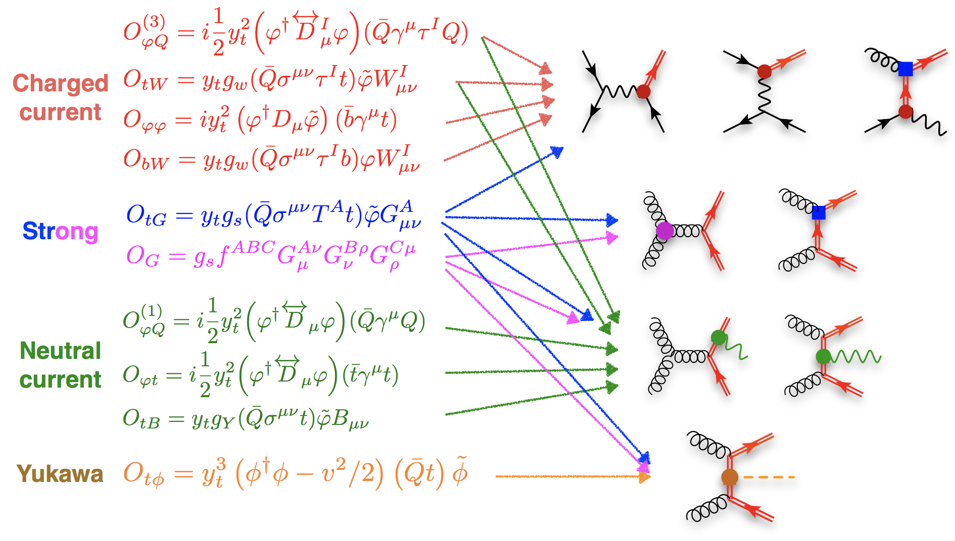
Figure 1: Two-quark operators entering the main production mechanisms, including single top, $t\overline{t}$, $t\overline{t}$+gauge boson and $t\overline{t}$+Higgs.

3 Observables

Global analyses in the literature often follow a bottom-up approach. They are based on observables measured under the SM assumptions, which are provided by experimental collaborations with statistical and systematic uncertainties in detail, allowing for combination with other measurements. The set of observables can be continuously extended as new measurements become available. The most important advantage of a bottom-up approach is that it can be easily followed by the theorists, and so any progress on the theory side, such as improved predictions and combination of new channels, can be immediately included in real analyses, and the corresponding impacts and improvements can be investigated in detail. This is useful for improving our interpretation of the theory framework and for identifying the most urgent needs. In the long term it should also be used as a preparation for a more advanced analysis, which could directly rely on data (i.e. without SM observables).

The most obvious observable used in a global fit is the total cross section. $t\overline{t}$ and single top cross sections are among the most precisely measured observables in top measurements, with respectively $\sim 5\%$ and $\sim 10\%$ errors. Recently at Run II the associated production channels such as $t\overline{t}+W/Z$ and single $t+Z$ also reached good precision. It should be pointed out that the experimental precision is not directly related to the constraining power of the measurement. One example is the four-top production process, which only has an upper limit of about 4.6 times the SM signal, but its cross section has a constraining power on $qqtt$ four-fermion operators that is already comparable with that from the $t\overline{t}$ measurements, due to an enhanced sensitivity to $qqtt$ operators [12]. Another example is that certain processes can benefit from unitarity violation due to electroweak operators, see a discussion in Ref. [13] about $tW$ scattering.

Differential cross sections play a special role in the SMEFT context. By naive power counting, one expects that the dim-6 operator contributions could scale like $E^{2}/\Lambda^{2}$. A differential measurement can thus isolate the phase space region with the best sensitivity. For example, it is well known that in $t\overline{t}$ production the $m_{tt}$ distribution is powerful, not only to constrain the four-fermion operators but also to distinguish them from deviations in other forms [7]. Sensitivity to deviations is achieved by balancing between small statistical uncertainty and systematic control for low mass regime but also small new physics-induced deviations, and the opposite situation for high-mass regime, see Ref. [14] for a more detailed discussion.

A related class of observables are the asymmetries in $t\overline{t}$ production. They have attracted extensive interest in the past due to apparent discrepancy between Tevatron data and SM predictions, which then failed to grow as more data were added. Taking into account the EW corrections and next-to-next-to-leading order QCD corrections, the remaining tension is below 1.5 $\sigma$. Nevertheless, these observables are useful in constraining four-fermion operators, as their contributions come from the tree level. At the linear order in $C/\Lambda^{2}$, there are only four independent degrees of freedom in all four-fermion operators, denoted as $C_{u,d}^{1,2}$. The cross sections and asymmetries are determined by $C_{u,d}^{1}+C_{u,d}^{2}$ and $C_{u,d}^{1}-C_{u,d}^{2}$ respectively, and so a useful strategy to bound the four-fermion operators is to combine cross section measurements with $A_{FB}$ or $A_{C}$ measurements, at two different energies (Tevatron and LHC), which is just enough to constrain all four directions [15].

The situation can be different if one starts to incorporate $\mathcal{O}(C^{2}/\Lambda^{4})$ terms. Ref. [15] has pointed out that within the current experimental bounds, these terms may not be negligible. In general, if the operator can be inserted once in the amplitude, an observable will be a quadratic function of the operator coefficients,

$$\sigma=\sigma_{SM}+\sum_{i}\frac{C_{i}\sigma_{i}}{\Lambda^{2}}+\sum_{i,j}\frac{C_{i}C_{j}\sigma_{ij}}{\Lambda^{4}}\,.$$ (16)

The fact that the quadratic term becomes dominant is often interpreted as the EFT becoming invalid, because naively one could expect that the dim-8 operators interfere at the same order $\mathcal{O}(\Lambda^{-4})$. Whether this is really the case is a model-dependent question. However, we should point out that there are motivations to incorporate dim-6 squared pieces, while neglecting dim-8 interference pieces. Suppose the underlying theory is described by one scale $M_{*}$ and one coupling $g_{*}$, so that

$$\frac{C}{\Lambda^{2}}\sim\frac{g_{*}^{2}}{M_{*}^{2}}\,.$$ (17)

The current limits on $C/\Lambda^{2}$ may imply a large $g_{*}$ is allowed if $M_{*}$ is to be kept above the scale of the measurement. In a process like $q\overline{q}\to t\overline{t}$, one could expect that dim-6 squared terms to dominate, as they are enhanced by four powers of $g_{*}$, while the dim-8 interferences to be subdominant, as they scale at most as $g_{*}^{2}$. The EFT expansion is still valid in this case, see Ref. [16] for more discussions. A comparison between dim-6 interference and the squared terms is not necessarily related to the validity of the EFT.

In $t\overline{t}$ production, if dim-6 squared terms are incorporated, the $C_{u,d}^{1,2}$ language is no longer valid. Instead, the full set of 14 four-fermion operators needs to be included

$$\begin{array}[]{ll}{O}^{(8,3)}_{Qq}=\left(\overline{Q}_{L}\gamma_{\mu}T^{a}\tau^{i}Q_{L}\right)\left(\overline{q}_{L}\gamma^{\mu}T^{a}\tau^{i}q_{L}\right)&{O}^{(1,3)}_{Qq}=\left(\overline{Q}_{L}\gamma_{\mu}\tau^{i}Q_{L}\right)\left(\overline{q}_{L}\gamma^{\mu}\tau^{i}q_{L}\right)\\ {O}^{(8,1)}_{Qq}=\left(\overline{Q}_{L}\gamma_{\mu}T^{a}Q_{L}\right)\left(\overline{q}_{L}\gamma^{\mu}T^{a}q_{L}\right)&{O}^{(1,1)}_{Qq}=\left(\overline{Q}_{L}\gamma_{\mu}Q_{L}\right)\left(\overline{q}_{L}\gamma^{\mu}q_{L}\right)\\ {O}^{(8)}_{td}=\left(\overline{t}_{R}\gamma_{\mu}T^{a}t_{R}\right)\left(\overline{d}_{R}\gamma^{\mu}T^{a}d_{R}\right)&{O}^{(1)}_{td}=\left(\overline{t}_{R}\gamma_{\mu}t_{R}\right)\left(\overline{d}_{R}\gamma^{\mu}d_{R}\right)\\ {O}^{(8)}_{tu}=\left(\overline{t}_{R}\gamma_{\mu}T^{a}t_{R}\right)\left(\overline{u}_{R}\gamma^{\mu}T^{a}u_{R}\right)&{O}^{(1)}_{tu}=\left(\overline{t}_{R}\gamma_{\mu}t_{R}\right)\left(\overline{u}_{R}\gamma^{\mu}u_{R}\right)\\ {O}^{(8)}_{tq}=\left(\overline{t}_{R}\gamma_{\mu}T^{a}t_{R}\right)\left(\overline{q}_{L}\gamma^{\mu}T^{a}q_{L}\right)&{O}^{(1)}_{tq}=\left(\overline{t}_{R}\gamma_{\mu}t_{R}\right)\left(\overline{q}_{L}\gamma^{\mu}q_{L}\right)\\ {O}^{(8)}_{Qd}=\left(\overline{Q}_{L}\gamma_{\mu}T^{a}Q_{L}\right)\left(\overline{d}_{R}\gamma^{\mu}T^{a}d_{R}\right)&{O}^{(1)}_{Qd}=\left(\overline{Q}_{L}\gamma_{\mu}Q_{L}\right)\left(\overline{d}_{R}\gamma^{\mu}d_{R}\right)\\ {O}^{(8)}_{Qu}=\left(\overline{Q}_{L}\gamma_{\mu}T^{a}Q_{L}\right)\left(\overline{u}_{R}\gamma^{\mu}T^{a}u_{R}\right)&{O}^{(1)}_{Qu}=\left(\overline{Q}_{L}\gamma_{\mu}Q_{L}\right)\left(\overline{u}_{R}\gamma^{\mu}u_{R}\right)\end{array}$$ (18)

assuming a U(2)^3(q,u,d) flavor symmetry on the first two generations. They represent 14 independent degrees of freedom in $t\overline{t}$ production, and can be derived from Eq. (9), by assigning appropriate flavor indices.

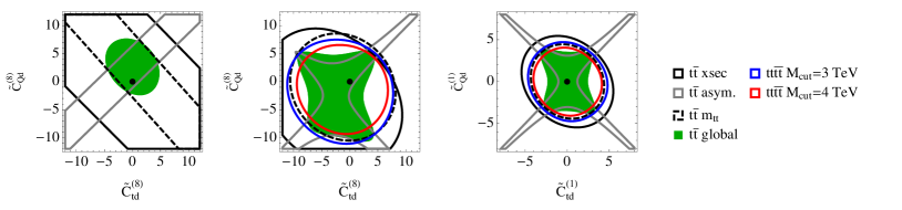
(a)                              (b)                              (c)

Figure 2: Constraints from $t\overline{t}$ cross section measurements (black solid), asymmetry measurements (gray), differential $m_{tt}$ distribution (black dashed), and four-top projection (blue and red) on selected four-fermion operators. Green shaded area corresponds to the combined result from $t\overline{t}$ measurements (see Ref. [12] for details). Operators in (a), (b) interfere with the SM amplitude, while those in (c) do not due to different color structures. Dim-6 squared and higher power terms are neglected in (a), but kept in (b), (c).

For illustration purpose, in Figure 2 we give the 95% CL constraints from cross section measurements, asymmetry measurements, a differential $m_{tt}$ distribution measurement, as well as bounds from four-top production. In Figure 2 (a) we show constraints on two color-octet operators, where only the dim-6 linear terms are kept. The constraints from cross section and $m_{tt}$ are orthogonal to those from asymmetry measurements, as they are determined by $C_{d}^{1}\pm C_{d}^{2}$ respectively. In Figure 2 (b) we consider the same operators, but without truncating the higher power terms of $C/\Lambda^{2}$. One can see that the allowed region from each experiment becomes quite different, as the dominant contributions become $(C_{d}^{1})^{2}\pm(C_{d}^{2})^{2}$. Interestingly, beyond the linear term, the four-top production cross section can place competitive constraints. In the plot we show the projections for $300$ fb^-1, with analysis cuts, $M_{cut}=3$ and 4 TeV, applied on the center of mass energy to ensure the validity of the EFT, see Ref. [12] for more details. Finally, in Figure 2 (c) we show similar constraints for two color singlet operators. These operators do not interfere with the SM at the dim-6 linear order, so no constraints can be obtained at that order. However, we can see that by including the dim-6 squared terms, the resulting constraints are even tighter than those of the color octet operators which interfere, due to a larger color factor.

Finally, the decay process also provides useful information. The most constrained observable is the $W$-helicity fraction. It is sensitive to the operator $O_{uW}^{(33)}$, but unlike the single-top cross section, it is virtually independent of the other operators that enter the $Wtb$ vertex, and thus providing complementary information. It should be noted that the $W$-helicity fraction is only a pseudo-observable, as the $W$ boson does not exist if the top decays through a four-fermion operator, which limits the applicability of this observable in a global fit. The total width, on the other hand, has not been measured to a very accurate level. This can be an issue because in principle one only measures the total cross section times the branching ratio, so the width could affect all cross section measurements if the theory framework used allows for exotic decay channels. In this respect it is useful to consider new methods that could improve the width measurement. For example, in Ref. [17] it has been proposed to use the $b$-charge identification as a way to remove the background and to improve the precision of the width measurement at high integrated luminosity.

A global fit that takes into account most of the existing measurements has been performed in Refs. [18, 19]. It is perhaps not surprising that no significant deviation from the SM has been found. Constraints are in general not very tight, in the sense that if one interprets the results using Eq. (17), and keeps $M_{*}$ above the energy of the measurement, then only a small window of the parameter space can be excluded if one requires the underlying theory to be perturbative [14]. Still, further improvements are expected at high integrated luminosity, as many differential distributions are still dominated by statistics, in particular in high mass regions where the EFT sensitivity is the largest.

4 NLO phenomenology

As we await for more results from experiments, the theory approach continues to improve. A lot of studies have appeared in the literature, some focusing on the matching of SMEFT to specific models (see, e.g., Ref. [20] and references therein), while others aiming at improving the precision of the theory prediction itself. We focus on the latter.

Given that the expectations from LHC Run-II on the attainable precision of the top-quark measurements are high, next-to-leading order (NLO) predictions for top-quark production channels are becoming relevant. Due to the large number of the relevant operators, we rely on many different observables predicted by each operator to effectively constrain every possible deviations from the SM. It is then important to know if and how these observables are modified by QCD corrections, in particular given that the top-quark is a colored particle.

Recently, NLO predictions for the SMEFT, matched with parton shower simulation, are becoming available in the MadGraph5_aMC@NLO framework [21], based on an automatic approach to NLO QCD calculation interfaced with shower via the MC@NLO method [22]. The dim-6 Lagrangian can be implemented with the help of a series of packages, including FeynRules and NLOCT [23, 24]. A model in the Universal FeynRules Output format [25] can be built, allowing for simulating a variety of processes at NLO in QCD. We briefly review the recent progresses in this direction. The interested readers may find more details in Refs. [26, 27, 28, 29, 11]. With these new implementations, top-quark analyses based on SMEFT are being promoted systematically to NLO in QCD.

Single top FCN production. The first step along this direction was made by Ref. [26], where the dim-6 operators that give rise to FCN interactions have been implemented in the framework described above. Single top production processes in association with a neutral gauge boson or a Higgs boson through FCN interactions have been computed at NLO in QCD, and corrections are found to be large. These results are relevant for phenomenology studies. In Ref. [30], we have performed a simple fit for all FCN interaction operators (including $2q2l$ ones), to demonstrate that in principle the framework allows for global fits to be performed at the NLO accuracy, given that corresponding tools are available. Some results are given in Figure 3.

Figure 3: Global constraints on FCN interactions, assuming $\Lambda=1$ TeV. The red (blue) allowed regions apply for a = 1 (2). A white mark indicates the individual limit. See Ref. [30] for more details.

Figure 4: 95% limits from single-top measurements, with LO or NLO predictions in EFT, assuming $\Lambda=1$ TeV, see Ref. [28] for more details.

Top-pair production. The chromo-dipole operator for the top quark, $O_{tG}\equiv y_{t}O_{uG}^{(33)}$, can be constrained by top-pair production. Assuming real operator coefficient, this calculation has been carried out at NLO in Ref. [27]. The $K$-factors for the total cross sections are found to be $1.1$, $1.4$, and $1.5$ respectively for Tevatron, LHC 8 TeV, and LHC 13/14 TeV. As a result, the current limits on the chromo-magnetic dipole moment of the top quark from direct measurements can be improved by roughly the same factors.

Single top production. Single top production has been computed in all three channels ($t$-channel, $s$-channel, and $tW$ associated production channel) at NLO in QCD, with operators $O_{\phi Q}^{(3)}\equiv y_{t}^{2}/2O_{\varphi q}^{3(33)}$, $O_{tW}\equiv y_{t}O_{uW}^{(33)}$, and $O_{qQ}^{(1,3)}\equiv O_{Qq}^{(1,3)}$ [28]. Inclusive $K$-factors typically range from $\sim 10\%$ to $\sim 50\%$. Scale uncertainties are significantly reduced. A three-operator fit based on cross section measurements have been performed. Results are shown in Figure 4, illustrating the improvements due to including QCD corrections.

Top-pair production in association with a gauge boson. At the LHC, the neutral couplings $ttZ$ and $tt\gamma$ can be probed by associated production of a top-quark pair with a neutral gauge boson $Z/\gamma$. The relevant operators are $O_{\phi Q}^{(1)}\equiv y_{t}^{2}/2O_{\varphi Q}^{33}$, $O_{\phi t}\equiv y_{t}^{2}/2O_{\varphi u}^{33}$, $O_{tB}\equiv y_{t}O_{uB}^{33}$, as well as $O_{tG}$, $O_{\phi Q}^{(3)}$, and $O_{tW}$. The corresponding NLO predictions are given in Ref. [29]. By studying the differential distributions, we find that the differential $K$-factor of the SM and that of the operator contribution can be quite different, therefore using the SM $K$-factor to rescale the operator contributions may not be a good approximation. The authors of Refs. [31, 32] have considered the same process taking into account the decay of the top quarks. Constraints from both high luminosity LHC and ILC are obtained, and significant improvements due to QCD corrections are found, as a consequence of the reduced scale uncertainty and the larger event rate due to a positive perturbative correction.

Figure 5: Projected constraints from $t\overline{t}H$, $H$, and $H+j$ at the LHC, 3000 fb^-1.

Figure 6: The QCD-NLO $K$-factors for the $e^{+}e^{-}\to t\overline{t}$ cross section, as a function of the centre-of-mass energy. The thickness of the bands covers QCD renormalization scale variation between $m_{t}/2$ and $2m_{t}$.

Top-pair production in association with a Higgs boson. The LHC provides the first chance to directly measure the interactions between the top quark and the Higgs boson through the associated production of a Higgs with $t\overline{t}$. In Ref. [11], this process has been computed at NLO including three operators: the chromo-dipole operator $O_{tG}$, the Yukawa operator $O_{t\phi}\equiv y_{t}^{3}O_{u\varphi}^{(33)}$, and the Higgs-gluon operator $O_{\phi G}\equiv y_{t}^{2}O_{HG}$. The QCD mixing of these three operators goes in the direction of increasing number of Higgs fields, i.e. $O_{tG}$ mixes into $O_{\phi G}$, and both of them mix into $O_{t\phi}$, but not the other way around. Based on the full NLO results, a combined fit using $t\overline{t}H$, $H$, and $H+j$ production has been performed to derive the current constraints and future projections (see Figure 5). The results imply that the Higgs measurements have started to become sensitive to the chromo-dipole coupling of the top, and so in future analyses the Higgs data will play a role in the study of top properties.

Top-pair production at $e^{+}e^{-}$ colliders. This process can be computed at NLO in QCD with not only the two-quark operators, but also the $2q2l$ operators, in both the $t\overline{t}$ and the $bW^{+}\overline{b}W^{-}$ final states. The global constraints from measurements at the future lepton colliders are under investigation [33]. In Figure 6 we illustrate the sizes of QCD corrections to the interference terms from different operators.

5 Outlook

So far we have only considered bottom-up analyses. Ideally, one could improve the experimental sensitivity by making use of the accurate SMEFT predictions and designing optimized experimental strategies in a top-down way. This is well established and widely used for concrete new physics models, but have been rarely considered in the standard SMEFT context. Given that the aim is to maximize the discovery potential of the LHC by combining state-of-the-art theoretical techniques and direct access to experimental data with full details, it is important to have all the theory set up ready before starting such an effort. The recent theoretical developments are paving the way towards this goal: we have discussed improvements on the precision and accuracy of theoretical predictions and corresponding tools, while another relevant issue, namely the optimization of the operator basis for top physics, is also under investigation (see [34] for some preliminary discussions). As a first step towards the final goal, preliminary studies on $t\overline{t}$ production based on a matrix-element method have shown improved sensitivity with respect to SM observable-based analysis [35]. We hope to see more progresses along this direction in the future to further push our reach in determining the top-quark properties.

ACKNOWLEDGEMENTS

I would like to thank C. Degrande, O. B. Bylund, G. Durieux, D. B. Franzosi, F. Maltoni, M. P. Rosello, I. Tsinikos, M. Vos, E. Vryonidou, and J. Wang for collaboration on many works mentioned in section 4.

References

- [1] D. Buttazzo, G. Degrassi, P. P. Giardino, G. F. Giudice, F. Sala, A. Salvio and A. Strumia, JHEP 1312, 089 (2013) doi:10.1007/JHEP12(2013)089 [arXiv:1307.3536 [hep-ph]].
- [2] S. Weinberg, Physica A 96, 327 (1979). doi:10.1016/0378-4371(79)90223-1
- [3] W. Buchmuller and D. Wyler, Nucl. Phys. B 268, 621 (1986). doi:10.1016/0550-3213(86)90262-2
- [4] C. N. Leung, S. T. Love and S. Rao, Z. Phys. C 31, 433 (1986). doi:10.1007/BF01588041
- [5] Q. H. Cao, J. Wudka and C.-P. Yuan, Phys. Lett. B 658, 50 (2007) doi:10.1016/j.physletb.2007.10.057 [arXiv:0704.2809 [hep-ph]].
- [6] C. Zhang and S. Willenbrock, Phys. Rev. D 83, 034006 (2011) doi:10.1103/PhysRevD.83.034006 [arXiv:1008.3869 [hep-ph]].
- [7] C. Degrande, J. M. Gerard, C. Grojean, F. Maltoni and G. Servant, JHEP 1103, 125 (2011) doi:10.1007/JHEP03(2011)125 [arXiv:1010.6304 [hep-ph]].
- [8] B. Grzadkowski, M. Iskrzynski, M. Misiak and J. Rosiek, JHEP 1010, 085 (2010) doi:10.1007/JHEP10(2010)085 [arXiv:1008.4884 [hep-ph]].
- [9] P. L. Cho and E. H. Simmons, Phys. Rev. D 51, 2360 (1995) doi:10.1103/PhysRevD.51.2360 [hep-ph/9408206].
- [10] F. Krauss, S. Kuttimalai and T. Plehn, Phys. Rev. D 95, no. 3, 035024 (2017) doi:10.1103/PhysRevD.95.035024 [arXiv:1611.00767 [hep-ph]].
- [11] F. Maltoni, E. Vryonidou and C. Zhang, JHEP 1610, 123 (2016) doi:10.1007/JHEP10(2016)123 [arXiv:1607.05330 [hep-ph]].
- [12] C. Zhang, arXiv:1708.05928 [hep-ph].
- [13] J. A. Dror, M. Farina, E. Salvioni and J. Serra, JHEP 1601, 071 (2016) doi:10.1007/JHEP01(2016)071 [arXiv:1511.03674 [hep-ph]].
- [14] C. Englert, L. Moore, K. Nordstrom and M. Russell, Phys. Lett. B 763, 9 (2016) doi:10.1016/j.physletb.2016.10.021 [arXiv:1607.04304 [hep-ph]].
- [15] M. P. Rosello and M. Vos, Eur. Phys. J. C 76, no. 4, 200 (2016) doi:10.1140/epjc/s10052-016-4040-x [arXiv:1512.07542 [hep-ex]].
- [16] R. Contino, A. Falkowski, F. Goertz et al, JHEP 1607: 144 (2016)
- [17] P. P. Giardino and C. Zhang, Phys. Rev. D 96, no. 1, 011901 (2017) doi:10.1103/PhysRevD.96.011901 [arXiv:1702.06996 [hep-ph]].
- [18] A. Buckley, C. Englert, J. Ferrando, D. J. Miller, L. Moore, M. Russell and C. D. White, Phys. Rev. D 92, no. 9, 091501 (2015) doi:10.1103/PhysRevD.92.091501 [arXiv:1506.08845 [hep-ph]].
- [19] A. Buckley, C. Englert, J. Ferrando, D. J. Miller, L. Moore, M. Russell and C. D. White, JHEP 1604, 015 (2016) doi:10.1007/JHEP04(2016)015 [arXiv:1512.03360 [hep-ph]].
- [20] Z. Zhang, JHEP 1705, 152 (2017) doi:10.1007/JHEP05(2017)152 [arXiv:1610.00710 [hep-ph]].
- [21] J. Alwall et al., JHEP 1407, 079 (2014) doi:10.1007/JHEP07(2014)079 [arXiv:1405.0301 [hep-ph]].
- [22] S. Frixione and B. R. Webber, JHEP 0206, 029 (2002) doi:10.1088/1126-6708/2002/06/029 [hep-ph/0204244].
- [23] A. Alloul, N. D. Christensen, C. Degrande, C. Duhr and B. Fuks, Comput. Phys. Commun. 185, 2250 (2014) doi:10.1016/j.cpc.2014.04.012 [arXiv:1310.1921 [hep-ph]].
- [24] C. Degrande, Comput. Phys. Commun. 197, 239 (2015) doi:10.1016/j.cpc.2015.08.015 [arXiv:1406.3030 [hep-ph]].
- [25] C. Degrande, C. Duhr, B. Fuks, D. Grellscheid, O. Mattelaer and T. Reiter, Comput. Phys. Commun. 183, 1201 (2012) doi:10.1016/j.cpc.2012.01.022 [arXiv:1108.2040 [hep-ph]].
- [26] C. Degrande, F. Maltoni, J. Wang and C. Zhang, Phys. Rev. D 91, 034024 (2015) doi:10.1103/PhysRevD.91.034024 [arXiv:1412.5594 [hep-ph]].
- [27] D. Buarque Franzosi and C. Zhang, Phys. Rev. D 91, no. 11, 114010 (2015) doi:10.1103/PhysRevD.91.114010 [arXiv:1503.08841 [hep-ph]].
- [28] C. Zhang, Phys. Rev. Lett. 116, no. 16, 162002 (2016) doi:10.1103/PhysRevLett.116.162002 [arXiv:1601.06163 [hep-ph]].
- [29] O. Bessidskaia Bylund, F. Maltoni, I. Tsinikos, E. Vryonidou and C. Zhang, JHEP 1605, 052 (2016) doi:10.1007/JHEP05(2016)052 [arXiv:1601.08193 [hep-ph]].
- [30] G. Durieux, F. Maltoni and C. Zhang, Phys. Rev. D 91, no. 7, 074017 (2015) doi:10.1103/PhysRevD.91.074017 [arXiv:1412.7166 [hep-ph]].
- [31] R. Rontsch and M. Schulze, JHEP 1407, 091 (2014) Erratum: [JHEP 1509, 132 (2015)] doi:10.1007/JHEP09(2015)132, 10.1007/JHEP07(2014)091 [arXiv:1404.1005 [hep-ph]].
- [32] R. Rontsch and M. Schulze, JHEP 1508, 044 (2015) doi:10.1007/JHEP08(2015)044 [arXiv:1501.05939 [hep-ph]].
- [33] G. Durieux, M. P. Rosello,M. Vos and C. Zhang, in progress.
- [34] G. Durieux, “TopEFT: Status of the proposal for a top EFT parameterization”, talk given at the LHC TOP WG meeting, 7 June 2017, https://indico.cern.ch/event/596233/contributions/2612653
- [35] S. Wertz, “Constraining high order operators in top pair events using the MEM”, talk given at the Mini-Workshop on “Matrix Element Methods for data analysis at the LHC”, http://agenda.irmp.ucl.ac.be/contributionDisplay.py?contribId=1&confId=2218