Dynamics of end-pulled polymer translocation through a nanopore

Abstract

We consider the translocation dynamics of a polymer chain forced through a nanopore by an external force on its head monomer on the trans side. For a proper theoretical treatment we generalize the iso-flux tension propagation (IFTP) theory to include friction arising from the trans side subchain. The theory reveals a complicated scenario of multiple scaling regimes depending on the configurations of the cis and the trans side subchains. In the limit of high driving forces $f$ such that the trans subchain is strongly stretched, the theory is in excellent agreement with molecular dynamics simulations and allows an exact analytic solution for the scaling of the translocation time ${\tau}$ as a function of the chain length $N_{0}$ and $f$. In this regime the asymptotic scaling exponents for ${\tau}\sim N_{0}^{\alpha}f^{\beta}$ are $\alpha=2$, and $\beta=-1$. The theory reveals significant correction-to-scaling terms arising from the cis side subchain and pore friction, which lead to a very slow approach to $\alpha=2$ from below as a function of increasing $N_{0}$.

Introduction. – Dynamics of polymer translocation through nanopores has become an active research topic in soft matter and biological physics during the last two decades Tapio_review ; Milchev_JPCM ; Muthukumar_book since the seminal experiment by Kasianowicz et al. in 1996 kasi1996 , and has many potential technological applications in biology, engineering and medicine just to name a few. In particular, translocation based setups have been suggested as rapid and inexpensive methods for DNA and other biopolymer sequencing. Motivated by these applications many experimental and theoretical meller2003 ; branton_PRL_2003 ; meller_biophys_j_2004 ; storm2005 ; branton2008 ; schadt2010 ; dimarzio1979 ; sung1996 ; muthu1999 ; chuang2001 ; metzler2003 ; kantor2004 ; grosberg2006 ; dubbeldam2007 ; sakaue2007 ; luo2008 ; sakaue2008 ; luo2009 ; bhatta2009 ; sakaue2010 ; rowghanian2011 ; saito2011 ; saito2012a ; saito2012b ; dubbeldam2011 ; ikonen2012a ; ikonen2012b ; ikonen2012c ; ikonen2013 ; jalal2014 ; jalal2015 ; jalal2017 ; unbiased_Slater_1 ; unbiased_Slater_2 ; unbiased_Slater_3 ; unbiased_Polson ; dubbeldam2013 ; Keyser_NatPhys_2006 ; Keyser_NatPhys_2009 ; Sischka ; Bulushev_NanoLett_2014 ; Bulushev_NanoLett_2015 ; Bulushev_NanoLett_2016 ; Menais_SciRep_2016 ; Santtu_EPJE_2009 ; Huopaniemi_2007 ; Panja_2008 studies have focused on the nature of the translocation dynamics. The three simplest basic translocation scenarios correspond to the cases of pore-driven, end-pulled, and unbiased setups unbiased_Slater_1 ; unbiased_Slater_2 ; unbiased_Slater_3 ; unbiased_Polson . In the pore-driven case an electric field, due to a voltage bias between the two sides of the membrane, acts on the monomers inside the pore. On the other hand, in the end-pulled case the polymer is pulled through a nanopore by either an optical or a magnetic tweezer Keyser_NatPhys_2006 ; Keyser_NatPhys_2009 ; Sischka ; Bulushev_NanoLett_2014 ; Bulushev_NanoLett_2015 ; Bulushev_NanoLett_2016 . End-pulled translocation has been suggested to be a good method to slow down and control the translocation process which is crucial for proper identification of the nucleotides in DNA sequencing kantor2004 ; Huopaniemi_2007 ; Santtu_EPJE_2009 .

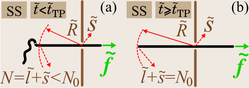
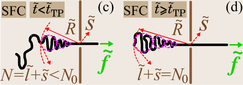
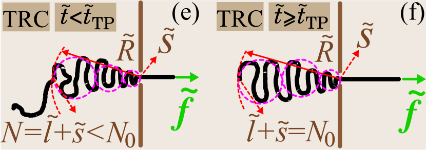
Figure 1: Schematic of the various possible translocation scenarios during the tension propagation (TP) stage for the trans side strong stretching (SST) regime. The driving force $\tilde{f}$ acts only on the head monomer of the polymer in the trans side. The length of polymer is $N_{0}$ and the number of beads that have been already translocated into the trans side is denoted by $\tilde{s}$. The number of total beads influenced by the tension is $N=\tilde{l}+\tilde{s}$ (in the TP stage $N<N_{0}$). In panel (a) the cis side subchain is also in the SS regime (SSC) during the TP stage. (b) The translocation process when the tension front reaches the end of the chain on the cis side in the SSC regime (post propagation stage (PP) where $N=N_{0}$). Panels (c) and (e) are the same as panel (a) but for the stem-flower (SFC) and trumpet (TRC) regimes in the cis side, respectively. Panels (d) and (f) are the same as panel (b) but for SFC and TRC, respectively. See text for details.

Over the last few years a quantitative theory for pore-driven translocation dynamics has been developed jalal2014 ; jalal2015 ; jalal2017 ; ikonen2012a ; ikonen2012b ; ikonen2012c ; ikonen2013 based on the idea of tension propagation by Sakaue sakaue2007 . The key role in this iso-flux rowghanian2011 tension propagation (IFTP) theory is played by the time-dependent friction of the cis side subchain that resists the driving and leads to different regimes of translocation dynamics depending on the strength of the driving force. Most recently, the theory has been extended to the case of semi-flexible polymer chains, where there’s an additional time-dependent frictional term arising from the trans side of the chain due to chain stiffness jalal2017 . To date the case of end-pulled translocation has not been theoretically treated beyond simple scaling arguments, however. Driven translocation processes are fundamentally far-from-equilibrium phenomena and scaling arguments alone cannot capture the relevant physics. To this end, in this work we present a proper theoretical treatment of the end-pulled setup based on the IFTP theory and augmented with extensive molecular dynamics (MD) simulations jalal2014 ; jalal2017 ; ikonen2012a ; ikonen2012b ; ikonen2012c . We show how the IFTP theory reveals the presence of translocation regimes that have not been previously considered. In the present work we concentrate in the limit of strong driving, and derive an exact scaling formula for the scaling of the translocation time with the chain length and the driving force. The theory is shown to be in excellent agreement with MD simulations of coarse-grained polymer chains.

Theory. – The IFTP theory has revealed that for the pore-driven case there are three different regimes of translocation dynamics corresponding to different force strengths, namely the strong stretching (SS) limit of high forces, the stem-flower (SF) regime of intermediate forces, and the trumpet (TR) regime of weak forces. For end-pulled chains this means that there is a complicated scenario of multiple regimes corresponding to different combinations of the chain configurations both on the cis and trans sides. For simplicity, in the present work we will consider only the case of high driving forces $\tilde{f}\gtrsim N_{0}$, where $\tilde{f}$ is the pulling force and $N_{0}$ is the chain length, such that the trans side subchain is fully straightened at all times during the translocation process which we call the trans-SS scenario here. Correspondingly, the cis side subchain can either be in the SS (SSC), stem-flower (SFC) or trumpet (TRC) regime. The other regimes will be discussed in future work.

In Fig. 1 we show the translocation regimes corresponding to the three different possible cis side subchain configurations. In the trans-SS regime it is sufficient to use the deterministic limit of the iso-flux Brownian dynamics tension propagation theory without the entropic force term ikonen2012a ; ikonen2012b ; jalal2014 ; jalal2015 ; jalal2017 . The corresponding equation of motion for $\tilde{s}$, the translocation coordinate which is the number of beads in the trans side, is given by

$$\tilde{\Gamma}(\tilde{t})\frac{d\tilde{s}}{d\tilde{t}}=\tilde{f},$$ (1)

where $\tilde{\Gamma}(\tilde{t})$ is the effective friction, and $\tilde{f}$ is the external driving force. We have recently extended the IFTP theory to the case of pore-driven semi-flexible chains jalal2017 and shown that the effective total friction $\tilde{\Gamma}(\tilde{t})$ must be written as $\tilde{\Gamma}(\tilde{t})=\tilde{\eta}_{\rm cis}(\tilde{t})+\tilde{\eta}_{\textrm{p}}+\tilde{\eta}_{\textrm{TS}}(\tilde{t})$, where the first two terms $\tilde{\eta}_{\rm cis}(\tilde{t})$ and $\tilde{\eta}_{\textrm{p}}(\tilde{t})$ are the cis side subchain and pore friction, respectively, and $\tilde{\eta}_{\textrm{TS}}(\tilde{t})$ is a new time dependent trans side friction that cannot be absorbed in the constant pore friction. We expect the trans side friction to play an important role for end-pulled polymers, too, and it needs to be explicitly taken into account.

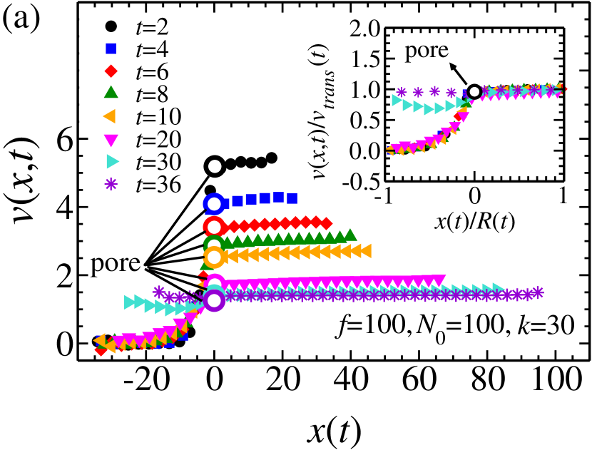
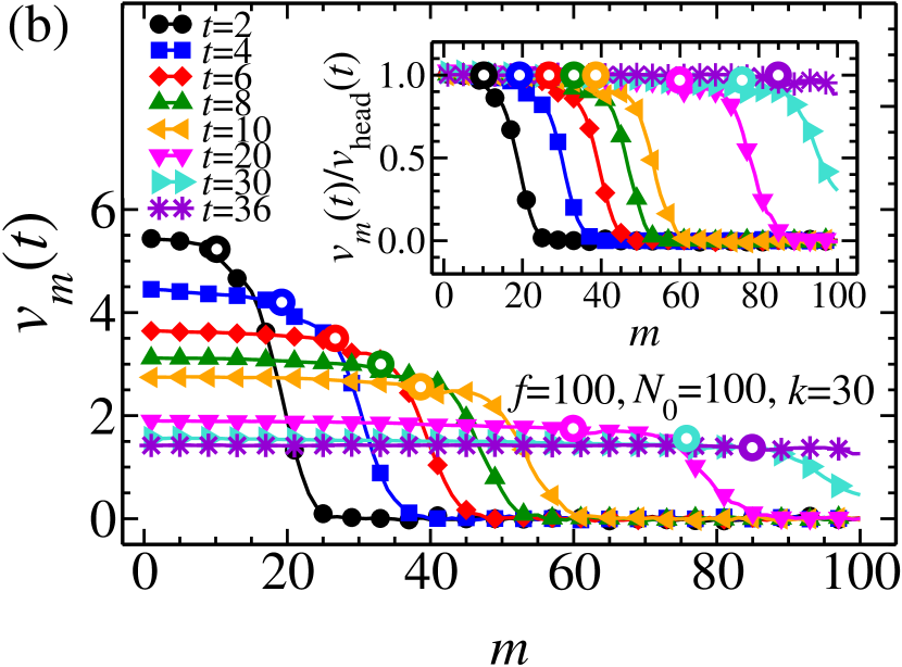
Figure 2: (a) Velocity perpendicular to the wall in the trans side and towards the pore in the cis side for individual monomers $v(x,t)$ as a function of the distance $x(t)$ at different times ${t}=2-{36}$. The empty circles show the pore locations at different times. Inset shows normalized velocity of individual monomers $v(x,t)/v_{\rm trans}(t)$ as a function of the normalized distance $x(t)/R(t)$. Here, $v_{{\rm trans}}(t)$ is the average velocity of the trans side sub-chain monomers and $R(t)$ is the amplitude of the tension front distance from the pore. The driving force acting on the head monomer is ${f}=100$, the chain length is $N_{0}=100$, and the location of the pore is denoted by an open black circle. (b) Velocity perpendicular to the wall in the trans side and towards the pore in the cis side of the monomers $v_{m}(t)$ as a function of the monomer number $m$ at different times ${t}=2-36$, where the empty colored circles show which monomer is inside the pore at each time. Inset shows the monomer velocity normalized by the head monomer velocity $v_{m}(t)/v_{\textrm{head}}(t)$ as a function of $m$. The values $m=1$ and 100 denote the head and tail monomers, respectively.

Within the IFTP theory the dynamics of the chain on the cis side is solved with the corresponding TP equations. To derive these we use the iso-flux approximation rowghanian2011 , where the monomer flux $\tilde{\phi}\equiv d\tilde{s}/d\tilde{t}$ on the mobile domain of the cis and trans sides and through the pore is constant in space but evolves in time. The tension front is located at distance $\tilde{x}=-\tilde{R}(\tilde{t})$ from the pore. Inside the mobile domain, the external driving force is mediated by the chain backbone from the head bead (head of polymer on which the external driving force acts) all the way to the pore at $\tilde{x}=0$ and then to the last mobile monomer $N$ located at the tension front (see Fig. 1). The magnitude of the tension force at distance $\tilde{x}$ can be calculated by considering the force balance relation $d\tilde{f}(\tilde{x}^{\prime})=-\tilde{\phi}(\tilde{t})d\tilde{x}^{\prime}$ for the differential element $d\tilde{x}^{\prime}$ that is located between $\tilde{x}^{\prime}$ and $\tilde{x}^{\prime}+d\tilde{x}^{\prime}$. By integrating the force balance relation over the distance from the head monomer to the pore on the trans side and then from the pore to $\tilde{x}$ on the cis side, the tension force is obtained as $\tilde{f}(\tilde{x},\tilde{t})=\tilde{f}_{0}-\tilde{\phi}(\tilde{t})\tilde{x}$, where $\tilde{f}_{0}\equiv\tilde{f}-\tilde{\eta}_{\textrm{p}}\tilde{\phi}(\tilde{t})-\tilde{\eta}_{\textrm{TS}}\tilde{\phi}(\tilde{t})$ is the force at the pore entrance on the cis side.

It is important to note that the tension front is always located on the cis side of the chain since the trans side is subject to a constant driving force. The same results have been verified for weaker and stronger forces. To illustrate this, in Fig. 2(a) we plot the velocity perpendicular to the wall in the trans side and towards the pore in the cis side for individual monomers $v(x,t)$ as a function of the distance $x(t)$ at different times ${t}=2-36$ during the translocation process, with ${f}=100$, spring constant $k=30$ and chain length $N_{0}=100$. Inset shows normalized velocity $v(x,t)/v_{{\rm trans}}(t)$ as a function of the normalized distance $x(t)/R(t)$, where $v_{{\rm trans}}(t)$ is the average monomer velocity of the trans side sub-chain and $R(t)$ is the amplitude of the tension front distance from the pore. Moreover, in Fig. 2(b) the velocity perpendicular to the wall in the trans side and towards the pore in the cis side for each monomer $v_{{m}}(t)$ is plotted as a function of the monomer number ${{m}}$ ($1\leq{m}\leq N_{0}$) with the same parameters as in Fig. 2(a) at different times $t=2-{36}$. As can be seen, in both panels (a) and (b) the velocity of the trans side monomers is almost constant and drops immediately close to the pore entrance on the cis side in the TP stage. This velocity drop occurs because of the reorientation of the mobile part of the chain on the cis side due to pulling. In the PP stage as time passes the velocity of the cis side sub-chain increases and finally becomes equal to that of the trans side sub-chain velocity. The results of the SFC and TRC regimes are shown to be in better quantitative agreement with the MD results than those from the SSC regime due to the occurence of this velocity change, as can bee seen in the waiting time distributions of Fig. 3.

In the SSC, SFC and TRC regimes the force balance equation is integrated over the mobile domain jalal2014 and the monomer flux is obtained as

$$\tilde{\phi}(\tilde{t})=\frac{\tilde{f}}{\tilde{R}(\tilde{t})+\tilde{\eta}_{\textrm{p}}+\tilde{\eta}_{{}_{\textrm{TS}}}^{\textrm{J}}},$$ (2)

where the superscript J refers to the SS, SFC or TRC regimes from hereon. By combining Eqs. (1) and (2), the effective friction can be written as

$$\tilde{\Gamma}(\tilde{t})=\tilde{R}(\tilde{t})+\tilde{\eta}_{\textrm{p}}+\tilde{\eta}_{{}_{\textrm{TS}}}^{\textrm{J}},$$ (3)

where in the high force limit $\tilde{\eta}_{{}_{\textrm{TS}}}^{\textrm{J}}=\tilde{s}$. This equation is formally the same as that for the pore-driven semi-flexible case jalal2017 , but the trans side friction term is different. In the present case it simply equals the distance of the head monomer of the chain from the pore because the trans side subchain is fully straightened here.

To determine the full solution for the time evolution of $\tilde{s}$ by Eqs. (1), (2) and (3), the position of the tension front $\tilde{R}(\tilde{t})$ must be known. To find this it should be noted that $\tilde{R}(\tilde{t})$ is equivalent to the root mean square of the end-to-end distance of the flexible chain $\tilde{R}_{N}=A_{\nu}N^{\nu}$, where $A_{\nu}=1.15$ and $\nu=0.588$ is the 3D Flory exponent. Therefore, using $\tilde{R}_{N}$ together with mass conservation which implies $N=\tilde{l}_{\textrm{J}}+\tilde{s}<N_{0}$ and $\tilde{l}_{\textrm{J}}+\tilde{s}=N_{0}$ in the TP and post propagation (PP) stages, respectively, we separately derive equations of motion for $\tilde{R}(\tilde{t})$ in the TP and PP stages. Here, the number of mobile beads on the cis side is defined as $\tilde{l}_{\textrm{J}}=\int_{\tilde{x}=0}^{\tilde{R}(\tilde{t})}\tilde{\sigma}_{\textrm{J}}(\tilde{x},\tilde{t})d\tilde{x}$, where the integration of the monomer number density $\tilde{\sigma}_{\textrm{J}}(\tilde{x},\tilde{t})$ is performed over the distance from the pore at $\tilde{x}=0$ to the tension front at $\tilde{x}=\tilde{R}(\tilde{t})$. The monomer number density is unity when the chain is straightened, and according to the blob theory it is given by $\tilde{\sigma}(\tilde{x})=|\tilde{f}(\tilde{x})|^{(\nu-1)/\nu}$ when the chain has the form of either a trumpet or a flower jalal2014 ; ikonen2012a . The quantity $\tilde{l}_{\textrm{J}}$ for different regimes can be obtained as jalal2014 $\tilde{l}_{\textrm{SS}}=\tilde{R}(\tilde{t})$, $\tilde{l}_{\textrm{SFC}}=\tilde{R}(\tilde{t})+(1-\nu)\tilde{\phi}(\tilde{t})^{-1}/(2\nu-1)$, and $\tilde{l}_{\textrm{TRC}}=\nu\tilde{\phi}(\tilde{t})^{(\nu-1)/\nu}\tilde{R}(\tilde{t})^{(2\nu-1)/\nu}/(2\nu-1)$. The time evolution of the tension front in the TP stage can be expressed as

$$\dot{\tilde{R}}(\tilde{t})\!=\!\frac{\nu A_{\nu}^{1/\nu}\tilde{R}^{(\nu-1)/\nu}{\cal{H}}_{\textrm{J}}}{1+\nu A_{\nu}^{1/\nu}\tilde{R}^{(\nu-1)/\nu}\tilde{\phi}(\tilde{t}){\cal{L}}_{\textrm{J}}},$$ (4)

and in the PP stage as

$$\dot{\tilde{R}}(\tilde{t})\!=\!\frac{{\cal{H}}_{\textrm{J}}}{\tilde{\phi}(\tilde{t}){\cal{L}}_{\textrm{J}}},$$ (5)

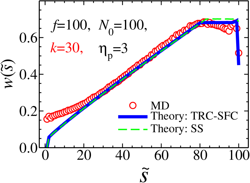
Figure 3: The waiting time distribution $w(\tilde{s})$ as a function of the translocation coordinate $\tilde{s}$. Here, the driving force is $f=100$, spring constant in the MD simulations is $k=30$, $N_{0}=100$ is the chain length and the pore friction in the theory is $\eta_{\textrm{p}}=3$. The red circles show the MD simulation results while the solid blue and the dashed green lines are the results from the IFTP theory for the combination of the TRC and SFC regimes, and for the SSC regime, respectively.

where the operators ${\cal{L}}_{\textrm{SS}}=-\tilde{\phi}(\tilde{t})^{-1}$, ${\cal{L}}_{\textrm{SFC}}=(\nu-1)[\tilde{R}(\tilde{t})+\tilde{\eta}_{\textrm{p}}+\tilde{s}]^{-1}\tilde{\phi}(\tilde{t})^{-2}/(2\nu-1)-\tilde{\phi}(\tilde{t})^{-1}$, ${\cal{L}}_{\textrm{TRC}}=\tilde{\phi}(\tilde{t})^{-(1+\nu)/\nu}\tilde{R}(\tilde{t})^{(\nu-1)/\nu}[\tilde{R}(\tilde{t})+\tilde{\eta}_{\textrm{p}}+\tilde{s}]^{-1}[\tilde{\phi}(\tilde{t})\tilde{R}(\tilde{t})(\nu-1)/(2\nu-1)-\tilde{f}]$, ${\cal{H}}_{\textrm{SS}}=\tilde{\phi}(\tilde{t})$, ${\cal{H}}_{\textrm{SFC}}=-\tilde{\phi}(\tilde{t})^{2}{\cal{L}}_{\textrm{SFC}}$, and ${\cal{H}}_{\textrm{TRC}}=-\tilde{\phi}(\tilde{t})^{2}{\cal{L}}_{\textrm{TRC}}+\tilde{\phi}(\tilde{t})-\tilde{\phi}(\tilde{t})[\tilde{\phi}(\tilde{t})\tilde{R}(\tilde{t})]^{(\nu-1)/\nu}$ corresponding to the three different regimes in Fig. 1. To find the full solution of the IFTP theory, in the TP stage Eqs. (1), (2), (3) and (4), and in the PP stage Eqs. (1), (2), (3) and (5) must be self-consistently solved.

Waiting time distribution. – To test the validity of the IFTP theory for the end-pulled case in Fig. 3 the monomer waiting time distribution $w(\tilde{s})$ (the time that each bead spends at the pore) is plotted as a function of the translocation coordinate $\tilde{s}$. The red circles show our MD data obtained using the same bead-spring model as in our previous works (the details can be found in the Supplementary). The solid blue line comes from the IFTP theory when the equations of motion are solved with a combination of the SFC and TRC regimes. This is determined based on the value of the force at the pore entrance in the cis side, namely if $\tilde{f}_{0}\gtrsim 1$ the equations must be solved in the SFC regime while for $\tilde{f}_{0}\lesssim 1$ we solve the equations in the TRC regime. The dashed green line represents the waiting time when the IFTP theory is solved in the SSC regime. As can be seen in Fig. 3, the combination of SFC and TRC matches perfectly with the MD data even in the PP stage. The dashed green curve for the SSC regime overestimates the waiting time in the PP stage because of the reorientation of the mobile part by the pore on the cis side in the MD simulations. Moreover, for small values of $\tilde{s}$ the solution of the IFTP theory underestimates the waiting time. This occurs in part because of bond stretching and also due to the beginning of the reorientation of the mobile part on the cis side as discussed in the theory subsection. As this discrepancy exists only for small values of $\tilde{s}$ and the main contribution of the waiting time and consequently the translocation time comes from the larger $\tilde{s}$ almost at the end of the TP stage, and over the whole PP stage, the IFTP theory correctly predicts the overall behavior of the translocation process.

Scaling exponents for translocation. – A fundamental characteristic of translocation dynamics is the scaling of the translocation time $\tilde{\tau}$ as a function of the chain length and the external driving force $\tilde{\tau}\propto\tilde{f}^{\beta}N_{0}^{\alpha}$, where $\alpha$ is the translocation exponent and $\beta$ is the force exponent.

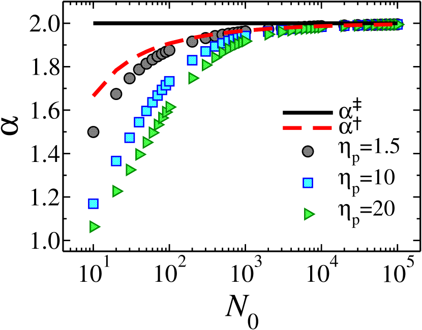
Figure 4: The effective translocation time exponent $\alpha$ as a function of chain length $N_{0}$ for various values of the pore friction $\eta_{\textrm{p}}=1.5$ (black circles), 10 (blue squares) and 20 (green triangles). The dashed red and the horizontal black solid lines represent the rescaled translocation exponents $\alpha^{{\dagger}}$ and $\alpha^{{\ddagger}}$, respectively.

Following Refs. jalal2014 ; jalal2017 we can derive an exact analytic expression for $\tilde{\tau}$, which is a sum of the TP ($\tilde{\tau}_{\mathrm{tp}}$) and PP ($\tilde{\tau}_{\mathrm{pp}}$) contributions to the translocation time as $\tilde{\tau}=\big{[}\int_{0}^{N_{0}}\tilde{R}_{N}dN+\tilde{\eta}_{\textrm{p}}N_{0}\big{]}/\tilde{f}+\tilde{\tau}_{\textrm{TS}}^{\textrm{J}}$. Since the trans side of the subchain is fully straightened for all the regimes of SSC, SFC and TRC (cf. Fig. 1), $\tilde{\tau}_{\textrm{TS}}^{\textrm{J}}=N_{0}^{2}/(2\tilde{f})$ and therefore

$$\tilde{\tau}=\frac{1}{\tilde{f}}\bigg{[}\frac{A_{\nu}}{\nu+1}N_{0}^{\nu+1}+\tilde{\eta}_{\textrm{p}}N_{0}+\frac{1}{2}N_{0}^{2}\bigg{]}.$$ (6)

Here, for the TP stage the conservation of mass is $N=\tilde{s}+\tilde{l}$ and the TP time can be obtained by integration of $N$ from $0$ to $N_{0}$, while in the PP stage the conservation of the mass gives $N=\tilde{s}+\tilde{l}=N_{0}$ and the PP time is solved by integration of $\tilde{R}$ from $\tilde{R}_{N_{0}}$ to zero. As can be seen in Eq. (6) the force exponent is $\beta=-1$. The first two terms in Eq. (6) are identical to the case of a pore-driven flexible chain jalal2014 , and the new term proportional to $N_{0}^{2}$ arises from the explicit trans side friction for the end-pulled case. While the asymptotic scaling exponent is $\alpha=2$, the two correction-to-asymptotic-scaling terms lead to pronounced crossover behavior due to the cis side and pore friction. To quantify the crossover scaling behavior in the high force limit, in Fig. 4 we plot the translocation time exponents $\alpha$, $\alpha^{{\dagger}}$, and $\alpha^{{\ddagger}}$ as a function of $N_{0}$ for various values of the bare pore friction. The two latter exponents have been defined by subtracting the correction terms as $\tilde{\tau}^{{\dagger}}=\tilde{\tau}-\tilde{\eta}_{\textrm{p}}N_{0}/\tilde{f}\sim N_{0}^{\alpha^{\dagger}}$ and $\tilde{\tau}^{{\ddagger}}=\tilde{\tau}-\big{[}\int_{0}^{N_{0}}\tilde{R}_{N}dN+\tilde{\eta}_{\textrm{p}}N_{0}\big{]}/\tilde{f}\sim N_{0}^{\alpha^{{\ddagger}}}$. For these typical parameters, asymptotic scaling is seen for very long chains only.

Summary. – We have studied the dynamics end-pulled polymer translocation through a nanopore by means of the proper analytical IFTP theory which reveals the existence of a complicated scenario depending on the strength of the driving force. Even in the case where the force is high enough such that the trans side of the chain is straight which is the focus here, there are three different regimes depending on the conformation of the cis side subchain. We have derived the corresponding equations of motion for the tension front propagation explicitly including the trans side friction. The theory shows excellent agreement with MD simulations for the waiting time distribution of the monomers, and allows an exact solution for the scaling of the translocation time as a function of the chain length and the driving force. As expected from simple scaling arguments, the theory recovers the asymptotic exponent $\alpha=2$, but with significant correction-to-scaling terms that come from the cis subchain and pore friction. Asymptotic scaling is recovered only for excessively long chains for typical parameter values.

Acknowledgements. – This work has been supported in part by the Academy of Finland through its Centers of Excellence Program under project nos. 251748 and 284621. The numerical calculations were performed using computer resources from the Aalto University School of Science “Science-IT” project, and from CSC - Center for Scientific Computing Ltd. The MD simulations were performed with the LAMMPS and GROMACS simulation softwares. S.C. and B.G. would like to thank IISER Pune and Centre for Development of Advanced Computing, Pune, India for providing the HPC facility. B.G. would like to acknowledge IISER Pune for fellowship. S. C. would like to thank DAE-BRNS, Grant No: (37(2)/14/08/2016-BRNS) for high performance computer cluster.

References

- (1) V. V. Palyulin, T. Ala-Nissila and R. Metzler, Soft Matter 10, 9016 (2014).
- (2) M. Muthukumar, Polymer Translocation (Taylor and Francis, 2011).
- (3) A. Milchev, J. Phys.: Condens. Matter 23, 103101 (2011).
- (4) J.J. Kasianowicz, E. Brandin, D. Branton and D.W. Deamer, Proc. Natl. Acad. Sci. 93, 13770 (1996).
- (5) A. Meller, J. Phys. Condens. Matter 15, R581 (2003).
- (6) A. F. Sauer-Budge, J. A. Nyamwanda, D. K. Lubensky and D. Branton, Phys. Rev. Lett. 90, 238101 (2003).
- (7) J. Mathe, H. Visram, V. Viasnoff, Y. Rabin and A. Meller, Biophys. J. 87, 3205 (2004).
- (8) A.J. Storm et al, Nano Lett. 5, 1193 (2005).
- (9) D. Branton, D.W. Deamer, A. Marziali et al., Nature Biotech. 26, 1146 (2008).
- (10) E.E. Schadt, S. Turner and A. Kasarskis, Hum Mol Gen 19, R227 (2010).
- (11) E. A. DiMarzio, C. M. Guttman and J. D. Hoffman, Faraday Discuss. Chem. Soc. 68, 210 (1979).
- (12) W. Sung and P.J. Park, Phys. Rev. Lett. 77, 783 (1996).
- (13) M. Muthukumar, J. Chem. Phys. 111, 10371 (1999).
- (14) J. Chuang, Y. Kantor and M. Kardar, Phys. Rev. E 65, 011802 (2001).
- (15) R. Metzler and J. Klafter, Biophys. J. 85, 2776 (2003).
- (16) Y. Kantor and M. Kardar, Phys. Rev. E 69, 021806 (2004).
- (17) A. Yu. Grosberg, S. Nechaev, M. Tamm and O. Vasilyev, Phys. Rev. Lett. 96, 228105 (2006).
- (18) J.L.A. Dubbeldam, A. Milchev, V.G. Rostiashvili and T.A. Vilgis, Europhysics Lett. 79, 18002 (2007).
- (19) T. Sakaue, Phys. Rev. E 76, 021803 (2007).
- (20) K. Luo, S.T.T. Ollila, I. Huopaniemi, T. Ala-Nissila, P. Pomorski, M. Karttunen, S.-C. Ying and A. Bhattacharya, Phys. Rev. E 78 050901(R) (2008).
- (21) T. Sakaue, in Proceedings of the 5th Workshop on Complex Systems, AIP CP, Vol. 982, p. 508 (2008).
- (22) K. Luo, T. Ala-Nissila, S.-C. Ying and R. Metzler, Europhys. Lett. 88, 68006 (2009).
- (23) A. Bhattacharya, W.H. Morrison, K. Luo, T. Ala-Nissila, S.-C. Ying, A. Milchev and K. Binder, Eur. Phys. J. E 29, 423 (2009).
- (24) T. Sakaue, Phys. Rev. E 81, 041808 (2010).
- (25) P. Rowghanian and A. Y. Grosberg, J. Phys. Chem. B 115, 14127 (2011).
- (26) T. Saito and T. Sakaue, Eur. Phys. J. E 34, 135 (2012).
- (27) T. Saito and T. Sakaue, Phys. Rev. E 85, 061803 (2012).
- (28) T. Saito and T. Sakaue, arXiv:1205.3861 (2012).
- (29) J. L. A. Dubbeldam, V. G. Rostiashvili, A. Milchev and T. A. Vilgis, Phys. Rev. E 85, 041801 (2012).
- (30) T. Ikonen, A. Bhattacharya, T. Ala-Nissila and W. Sung, Phys. Rev. E 85, 051803 (2012).
- (31) T. Ikonen, A. Bhattacharya, T. Ala-Nissila and W. Sung, J. Chem. Phys. 137, 085101 (2012).
- (32) T. Ikonen, J. Shin, W. Sung and T. Ala-Nissila, J. Chem. Phys. 136, 205104 (2012).
- (33) T. Ikonen, A. Bhattacharya, T. Ala-Nissila, W. Sung, Europhys. Lett 103, 38001 (2013).
- (34) J. Sarabadani, T. Ikonen and T. Ala-Nissila, J. Chem. Phys. 141, 214907 (2014).
- (35) J. Sarabadani, T. Ikonen and T. Ala-Nissila, J. Chem. Phys. 143, 074905 (2015).
- (36) J. Sarabadani, T. Ikonen, H. Mökkönen, T. Ala-Nissila, S. Carson and M. Wanunu, Sci. Rep. 7, 7423 (2017).
- (37) H. W. de Haan and G. W. Slater, Phys. Rev. E 81, 051802 (2010).
- (38) H. W. de Haan and G. W. Slater, J. Chem. Phys. 136, 204902 (2012).
- (39) M. G. Gauthier and G. W. Slater, Phys. Rev. E 79, 021802 (2009).
- (40) J. M. Polson and A. C. M. McCaffrey, J. Chem. Phys. 138, 174902 (2013).
- (41) J. L. A. Dubbeldam, V. G. Rostiashvili, A. Milchev and T. A. Vilgis, Phys. Rev. E 87, 032147 (2013).
- (42) U. F. Keyser, B. N. Koeleman, S. V. Drop, D. Krapf, R. M. M. Smeets, S. G. Lemay, N. H. Dekker, and C. Dekker, Nature Physics 2, 473 (2006).
- (43) U. F. Keyser, N. H. Dekker, C. Dekker and S. G. Lemay, Nature Physics 5, 347 (2009).
- (44) A. Sischka, A. Spiering, M. Khaksar, M. Laxa, J. König, K.-J. Dietz and D. Anselmetti, J. Phys: Cond. Matter 22, 454121 (2010).
- (45) R. D. Bulushev, L. J. Steinbock, S. Khlybov, J. F. Steinbock, U. F. Keyser and A. Radenovic, Nano Letters 14, 6606 (2014).
- (46) R. D. Bulushev, S. Marion and A. Radenovic, Nano Letters 15, 7118 (2015).
- (47) R. D. Bulushev, S. Marion, E. Petrova, S. J. davis, S. J. Maerkl and A. Radenovic, Nano Letters 16, 7882 (2016).
- (48) T. Menais, S. Mossa and A. Buhot, Sci. Rep. 6, 38558 (2016).
- (49) I. Huopaniemi, K. Luo, T. Ala-Nissila and S.-C. Ying, Phys. Rev. E 75, 061912 (2007).
- (50) S. T. T. Ollila, K. F. Luo, T. Ala-Nissila and S.-C. Ying, Eur. Phys. J. E 28, 385 (2009).
- (51) D. Panja and G. T. Barkema, Biophysical J. 94, 1630 (2008).