Relativistic numerical cosmology with Silent Universes
Abstract
Relativistic numerical cosmology is most often based either on the exact solutions of the Einstein equations, or perturbation theory, or weak-field limit, or the BSSN formalism. The Silent Universe provides an alternative approach to investigate relativistic evolution of cosmological systems. The silent universe is based on the solution of the Einstein equations in 1+3 comoving coordinates with additional constraints imposed. These constraints include: the gravitational field is sourced by dust and cosmological constant only, both rotation and magnetic part of the Weyl tensor vanish, and the shear is diagnosable. This paper describes the code simsilun (free software distributed under the terms of the reposi General Public License), which implements the equations of the Silent Universe. The paper also discusses applications of the Silent Universe and it uses the Millennium simulation to set up the initial conditions for the code simsilun. The simulation obtained this way consists of 16,777,216 worldlines, which are evolved from to . Initially, the mean evolution (averaged over the whole domain) follows the evolution of the background CDM model. However, once the evolution of cosmic structures becomes nonlinear, the spatial curvature evolves from to at the present day. The emergence of the spatial curvature is associated with and being smaller by approximately compared to the CDM.
Keywords: cosmology: theory – cosmological parameters – large-scale structure of Universe – methods: numerical
1 Introduction
The year 2017 marked the 100th anniversary of relativistic cosmology that started with Einstein’s cosmological model (Einstein, 1917) and de Sitter’s lecture On the relativity of inertia delivered on 31th of March 1917, at the Meeting of the Royal Netherlands Academy of Arts and Sciences (de Sitter, 1917). The following years brought new cosmological solutions of the Einstein equations, such as the solutions found by Friedmann (1922, 1924) and Lemaître (1927). These solutions were based on the assumption of homogeneity and isotropy, further investigated by Robertson (1929, 1933) and Walker (1935) (hence the name FLRW models). The FLRW models also include, as a spatial case, the spatially flat Einstein-de Sitter model (Einstein & de Sitter, 1932).
Inhomogeneous but isotropic solutions of the Einstein equations were first found by Lemaître (1933), and then further studied by Tolman (1934) and Bondi (1947) (hence the name LTB models). These spherically symmetric models were then generalised by Ellis (1967) to include other -symmetric spacetimes. Soon Ellis & MacCallum (1969) investigated anisotropic but homogeneous solutions of the Einstein equations, the so called Bianchi models. The most general (currently known) cosmological solution of the Einstein equations that is both inhomogeneous and anisotropic was found by Szekeres (1975) and then generalised (to include gradient-free pressure) by Szafron (1977). The Szekeres-Szafron solutions are quite general and contain in special limits the LTB and FLRW models and also the Schwarzschild solution (Plebański & Krasiński, 2006). (For a review on different inhomogeneous cosmological solutions and their applications see the monograph by Krasinski (1997) and the review article by Bolejko et al. (2011)).
In parallel to exact solutions, a perturbative approach had also been developed during this time, especially throughout 1980s, with the focus on a covariant approach to perturbations (Bardeen, 1980; Ellis & Bruni, 1989). However, the perturbative approach requires a stable background, and so it may not be accurate if the growth of nonlinear structures affects the evolution of the background, the so called cosmological backreaction (Clarkson et al., 2009). Although studies of backreaction within the perturbative schemes are being developed (Buchert & Ostermann, 2012; Buchert et al., 2013; Alles et al., 2015), currently most studies and applications of the perturbative schemes focus on statistical properties of matter on very large scales, in particular on the nonlinear evolution of the matter power spectrum (Baumann et al., 2012; Baldauf et al., 2015a, b; Blas et al., 2016).
In 1960s and 1970s an alternative approach to study relativistic and nonlinear cosmological systems started being developed. This approach is based on 1+3 split (Ellis, 1971, 2009) and it proved to be quite a powerful tool to study properties of relativistic cosmological systems. The two most known developments that followed from this approach are: models with the Local Rotational Symmetry (LRS) (van Elst & Ellis, 1996) and Silent Universes (Bruni et al., 1995; van Elst et al., 1997). The class II of the LRS models111The LRS models can be divided into 3 categories, with class I generalising the Gödle solution and class III generalising the Bianchi models. and silent universes have a common subset in the LTB models. The class II reduces to the LTB family when pressure and geodesic acceleration vanish (), and the silent universe reduces to the LTB solution when the isotropy is imposed.
After the initial period of interest around the silent universes, the enthusiasm faded. In mid 1990s it was hoped that this approach would allow to trace the evolution of cosmological systems far into the nonlinear regime. However, limitations due to diagonalisable shear tensor and vanishing magnetic part of the Weyl tensor (Maartens et al., 1997), as well as the absence of rotation, showed that one cannot trace the evolution too far into the nonlinear regime (Ellis & Tsagas, 2002). Also, at that time Newtonian numerical simulations started gaining momentum proving they can be very useful to study highly nonlinear stages of evolution of cosmic structures and their properties (Navarro et al., 1996). By mid 2000s the Newtonian simulations provided community with synthetic universes such as for example the Millennium simulation (Springel et al., 2005). However, -body simulations are based on Newtonian cosmology and use periodic boundary conditions, which means that the global evolution must follow the FLRW evolution (Buchert & Ehlers, 1997). This issue is important for relativistic cosmologists, who since mid 1980s have been investigating the phenomenon of backreaction (for a review on backreaction and the survey of opinions see a review article by Bolejko & Korzyński (2017)). The phenomenon of backreaction describes how the global evolution of the Universe is affected by the nonlinear growth of cosmic structures. So although Newtonian simulations are very successful in explaining small scale processes such as for example properties of galaxies (Vogelsberger et al., 2014; Laigle et al., 2015), they have limited applicability to studies of the global evolution of the universe that undergoes a nonlinear growth of structures (Buchert, 2017).
The extensions of the Newtonian -body simulations to include post-Newtonian corrections have been investigated and it was shown that the mean evolution is well approximated by the Friedmannian evolution (Adamek et al., 2013; Adamek et al., 2014; Adamek et al., 2016). This is related to the fact that periodic boundary conditions impose a constraint on the global spatial curvature and force it to vanish (Adamek et al., 2017). This is an important observations, because it is the global spatial curvature that has been identified as a key element of backreaction (Ellis & Buchert, 2005; Buchert & Carfora, 2008; Buchert et al., 2009; Roy et al., 2011; Bolejko, 2017b, a).
Recently, Rácz et al. (2017) suggested to include a Buchert-type backreaction to evaluate expansion rate of -body domains based on their cosmological environment. This has been extended by Roukema (2017) to include the Relativistic Zeldovich Approximation (RZA) to describe the expansion rate of various domains within -body simulations and to make the treatment of virialisation explicit rather than implicit. The RZA is a powerful tool (Kasai, 1995; Morita et al., 1998; Rampf & Buchert, 2012; Buchert et al., 2013; Alles et al., 2015), which is a general-relativistic approximation that goes far beyond standard perturbation theory, and for example successfully describe collapsing structures and predicts the mass function that to the first order is comparable to -body simulations, but is relativistic in origin (Ostrowski et al., 2016, 2017).
This new approach of extending the -body simulations has recently sparked a debate (Kaiser, 2017; Buchert, 2017; Roukema, 2017). There are many issues that need further examination, such as the constraints that follow from periodic boundary conditions, the implementation of expansion rates that vary spatially among local domains, the emergence of the average spatial curvature, and virialisation. Therefore, it seems that in order to thoroughly understand the backreaction phenomenon we will require a fully relativistic description of the evolution of cosmological systems, which most likely will only be achieved by the means of numerical relativity.
In the recent years, there have been serious developments of relativistic numerical cosmology based on the Einstein toolkit (Löffler et al., 2012) and the Baumgarte-Shapiro-Shibata-Nakamura (BSSN) formalism (Shibata & Nakamura, 1995; Baumgarte & Shapiro, 1999). The results obtained by Bentivegna & Bruni (2016), Mertens et al. (2016), and Macpherson et al. (2017) are impressive and encouraging. However, due to presence of shell crossings and due to the fact that these simulations are significantly CPU expensive, their applications is currently quite limited. On the other hand, silent cosmology can provide a viable alternative, at least until the relativistic numerical cosmology is fully developed. The code simsilun described in Sec. 3 is very fast — the evolution of 10,000 worldliness with non-extreme densities, over Gyr, takes 1 second on a 8-core CPU machine with the openMP parallelisation. The silent universes can provide a benchmark for full numerical cosmology, at least in the mildly nonlinear regime.
The structure of the paper is as follows: Sec. 2 provides a derivation of the silent universe; Sec. 3 describes the code simsilun; Sec. 4 presents the results of the Simsilun simulation and shows that a natural consequence of the relativistic evolution is the emergence of spatial curvature , and slightly lower values and compared to the CDM model; Sec. 5 presents the conclusions.
2 ‘Silent’ approach to relativistic cosmology
2.1 Relativistic evolution of a cosmic fluid
Below the equations for the silent universe are derived. The material is compiled from the work by Ellis (1971, 2009), Ehlers (1993), van Elst et al. (1997), Plebański & Krasiński (2006), and Tsagas et al. (2008).
The silent universe and its evolutionary equations are derived using the 1+3 split (time+space) and comoving gauge. Within this approach one assumes existence a unique vector filed that can be associated with the flow of matter (this could be an average velocity field of a given domain). Then, worldlines of particular domains (and time) are defined as lines that are tangent to , and space is defined as a surface orthogonal to . A cosmological fluid with its velocity can then be described with the following energy momentum tensor
| (1) |
where is energy density, is pressure, is the anisotropic stress tensor (), is the heat-flow vector (), and is the spatial part of the metric in 3+1 split . Introducing the following notation and , the gradient of the velocity field can be written as
| (2) |
where is rotation, is shear (the angle bracket is the projected symmetric trace-free part: , is expansion, and is acceleration. The evolution of the fluid follows from the conservation equations
| (3) | |||
| (4) |
and the evolution of the velocity field follows from the Ricci identities ()
| (5) | |||
| (6) | |||
| (7) |
where , , and is the electric part of the Weyl tensor , which together with the magnetic part is defined as , and . The evolution of the Weyl curvature follows from the Bianchi identities ()
| (8) | |||
| (9) |
The above equations provide the description of the evolution of a cosmic fluid. Thus, the state of the cosmic fluid is defined by properties of the fluid (density , pressure and , and energy transfer ), its velocity filed (expansion rate , shear , rotation , and acceleration ), and spacetime curvature (electric and magnetic parts of the Weyl tensor). In order to evolve the fluid (i.e. solve eqs. (3)–(9)) one also needs to specify the initial conditions and satisfy the spatial constraints, i.e. spatial parts of the Ricci identities
| (10) | |||
| (11) | |||
| (12) |
and Bianchi identities
| (13) | |||
2.2 Evolution of the irrotational silent universe
Irrotational silent universe is such a solution of the above equations, where each worldline evolves independently of other worldlines, and apart from the initial constraints there is no communication between the worldlines, i.e. no pressure gradients, no energy flux, no gravitational radiation:
These constraints have strong implications. For example from Bianchi and Ricci identities with follows that
which means that inhomogeneous models with diagonalisable the shear and electric part of the Weyl tensor have only 1 independent component of the shear and only 1 independent component of the electric part of the Weyl tensor (to be precise: 2 eigenvalues are identical, and the third is fixed by the condition of vanishing trace). This implies that the Petrov type I models are ruled out (for more details see a rigorous derivation by van Elst et al. (1997)). Thus the most general silent inhomogeneous models are Petrov type D, and so the shear tensor and the electric Weyl tensor can be written as
| (15) |
where where is a space-like unit vector aligned with the Weyl principal tetrad. As a result the fluid equations (3)–(9) reduce only to 4 scalar equations (Bruni et al., 1995; van Elst et al., 1997)
| (16) | |||
| (17) | |||
| (18) | |||
| (19) |
It is interesting to note that initially it was thought that the evolution of the silent universe would be described by 6 scalars: 1 density, 1 expansion rate, 2 for the shear tensor, and 2 for the electric part of the Weyl tensor (Bruni et al., 1995), but then it was proved by van Elst et al. (1997) and also by Maartens et al. (1997) that the constraints (12) and (LABEL:brc5) reduce the number of scalars to 4. Recently, Gierzkiewicz & Golda (2016) showed that for 4 scalars the evolution equations are completely integrable, but in the case of 6 scalars the system is not integrable, i.e. the Darboux polynomials method yields only 1 first integral.
2.3 Initial conditions, spatial constraints, and the approximation of the Simplified Silent Universe
When specifying the initial conditions one needs to make sure that the spatial constraints (10)–(LABEL:brc5) are satisfied. If these constraints are initially satisfied, they will be preserved in the course of the evolution (van Elst et al., 1997; Maartens et al., 1997). These conditions involve covariant derivatives so in order to satisfy them one needs to know the Christoffel symbols, which usually implies knowledge of the metric. It is possible to replace the terms that involve covariant derivatives with other quantities, consequently replacing them with algebraic relations (Sussman & Bolejko, 2012), but eventually one either needs to know the metric to evaluate these terms or use some other algorithm to constrain these quantities. Below, such an algorithm is presented, and it is based on several approximations. We first start with writing down the perturbations for the density filed
| (20) |
where is the background density, and is the density contrast. In the early universe matter density is much larger than the contribution from the cosmological constant, and so the universe (or the CDM model, which is used in this paper) evolves as the Einstein-de Sitter model. Assuming that the perturbations are small and dominated by the growing mode (Peebles, 1980) the expansion rate is
| (21) |
Inserting (15) to (10) and (LABEL:brc4), and assuming that the early universe is well approximated by the Einstein-de Sitter background (i.e. ) we get that
| (22) | |||
| (23) |
where above it was also assumed that the shear is a perturbation, so . Comparing the right hand sides of the above equations and neglecting higher order terms (such as ), the above equations reduce to
| (24) |
Up to this stage, the explicit knowledge of the metric was not essential. However, in order to find the relation for or , which is needed to provide all 4 initial conditions, one needs to know the metric. Without the explicit knowledge of the metric, one can only rely on further approximations. Here we are going to apply an approximation that is based on the exact formula for the quasi-local perturbations and averages (Sussman & Bolejko, 2012), which is
| (25) |
Although this relation is exact for the quasi-local quantities, it is not the exact relation for local quantities. For local quantities this relation follows if one assumes that locally the spacetime is flat (), then one can integrate eq. (10) and arrive at the above formula. This allows us to close all the equations and write down the formulae for the initial conditions
| (26) | |||
| (27) | |||
| (28) | |||
| (29) |
where the subscript denotes initial values, and is the initial density contrast. The first equations is just a definition of a perturbation . The second one is exact as long as the perturbations are small and the background is well approximated by the Einstein-de Sitter model (this is satisfied in the early universe). The relation between the shear and the Weyl curvature is also based on the linear perturbations around the Einstein-de Sitter model. However, eq. (28) is more than just a linear approximation. This is an exact relation for quasi-local quantities (Sussman & Bolejko, 2012) but for local quantities it is an approximation. This approximation reduces the richness of all possible initial conditions that enter via (10) to a single quantity . Therefore, the above set of initial conditions is referred to as the Simplified Silent Universe, and the code that implements these relations is named simsilun.
2.4 Comparison with the Szekeres model
The Szekeres model is the most general, explicit solution that belongs to the class of the silent universes. Therefore, it can be used to test the above approximations, which form the basis of the Simplified Silent Universe. The metric of the quasispherical Szekeres model is usually represented in the following form (Hellaby, 1996)
| (30) |
where , , and is an arbitrary function of . The function is given by
| (31) |
where the functions , , . The evolution of the system follows from the Einstein equations and reduces to a single equation
| (32) |
where , is the cosmological constant, and is an arbitrary function. The above equation can be integrated and used to define one more arbitrary function, i.e. the bang time function
| (33) |
The fluid scalars: density , expansion , shear , and Weyl curvature can be expressed in terms of the function and the arbitrary functions , and (Hellaby & Krasiński, 2002)
| (34) | |||
| (35) | |||
| (36) | |||
| (37) |
Thus, to calculate the evolution of the system and evaluate the fluid scalars (density , expansion , shear , and Weyl curvature ) one needs to know the form of the arbitrary functions , , and (to get ), and and to get the evolution of . For the purpose of this Section, the function is set to be
| (38) |
, , and , and and , and km s-1 Mpc-1, and the cosmological constant is set to be , where (Planck Collaboration et al., 2016). The function is fixed by the condition of a uniform age of the universe , so that it corresponds to existence of pure growing modes (Bolejko et al., 2009; Sussman, 2013). Finally, the functions that define the dipole are
| (39) |
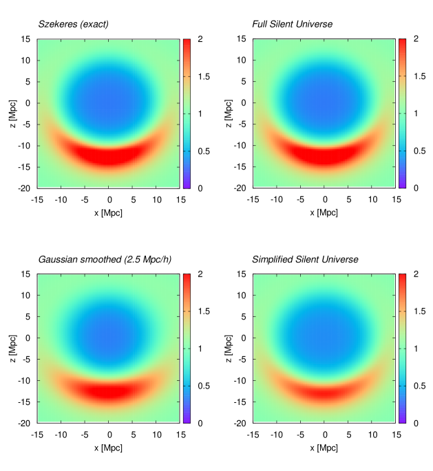
The model is specified at the last scattering instant and its evolution is calculated up to the present instant by integrating eq. (32). The present-day density distribution is presented in the upper left panel of Fig. 1. Then, at the initial instant, the initial values for , , , and were obtained from eqs. (34)–(37). These initial conditions were then used to calculate the evolution of the system (16)–(19), and the resulted present-day density distribution is presented in the upper right panel of Fig. 1. The numerical solution of eqs. (16)–(19) with the initial conditions given by eqs. (26)–(29), which corresponds to Simplified Silent Universe is presented in the lower right panel of Fig. 1. For comparison, the Gaussian smoothed density distribution of the Szekeres model (upper left) is presented in the lower left panel of Fig. 1. As seen, there is a reasonably good agreement between the full solution and the simplified solutions, which justifies the application of the Simplified Silent Universe.
3 The code: simsilun
The code is available via the Bitbucket repository222https://bitbucket.org/bolejko/simsilun. The code is written in Fortran. The algorithm on which the code is based is presented in Fig. 2. The code consists of 3 subroutines: get_parameters (the subroutine that contains the cosmological parameters and other model parameters), initial_data (the subroutine that reads the initial data such as: initial and final redshift/instant, initial background’s density and expansion rate, and initial density contrast), and silent_evolution (the subroutine that calculates the evolution). The evolution is calculated by numerically solving eqs. (16)–(19) with the 4th order Runge–Kutta method, and the initial conditions given by eqs. (26)–(29).
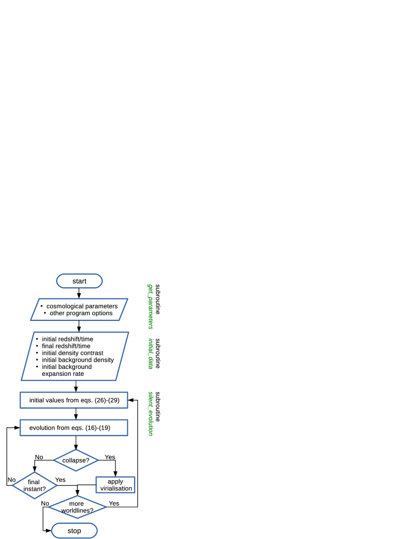
Within the silent universe, vorticity and pressure gradients are absent. Consequently, once the density contrast is too large and matter starts to collapse, there is nothing that could prevent the singularity. In order to prevent the singularity, some virialisation mechanism needs to be implemented. Since the model lacks the rotation and gradients, the virialisation needs to be implemented externally. In the code simsilun three types of virialisation mechanisms are implemented:
-
•
Stop at the turnaround
The code stops at the turnaround, i.e. when becomes negative. The fluid scalars are recoded as they are at this instant, and the expansion rate is set to zero, . The code then assumes that these quantities are ‘frozen’ and do not change across the cosmic evolution any more.
-
•
Stop near the singularity
The code stops at the singularity, and restores the fluid scalars as they were 2 numerical steps before the singularity333Since the code reaches the singularity, users are advised to check how their compilers handle it. The code was tested with ifort and gfortran and these compilers are able to handle NaN and restore the fluid scalars as they were before the singularity.. These values are then recoded, the expansion rate is set to zero, , and the code assumes that these quantities do not change any more.
-
•
Virialised halo
Here it is assumed that the end point of a collapse is a virialised halo with the NFW profile. The volume of the halo is , where is matter density of the background model (here it is the CDM model), , and is the mass (Navarro et al., 1996; Jenkins et al., 2001). Since the mass is conserved throughout the evolution its value is the same as at the initial instant, , where is the initial density and initial volume. Matter density evolves with time, , so the volume occupied by the virialised halo also evolves with time. The code stops and the turnaround, and replaces the collapsing region with a virialised halo. To account for the transition zone between the virialised halo and the surrounding universe it is assumed that the volume of this element is , and so the density of the cell is . The other fluid scalars are assumed to be zero, ie. .
The code can be run as it is stands, without any modifications. However, the user is encouraged to modify the code to meet any specific needs. For example, in the code the initial data is specified as a vector of 2000 different worldliness. This part can easily be modified by the user to include any other data (as for example in Sec. 4). Similarly, the initial conditions for , , , and are based on the conditions for the Simplified Silent Universe (26)–(29). This part can also be modified by the user to include the full exact solution of (10) and (LABEL:brc4) (as for example in Sec. 2.4).
After compiling and running the code (see the file readme for instructions) the code produces results presented in Fig. 3. Figure 3 shows the present-day density (to be precise it is so that it shows well on a log-scale plot) obtained from the code. It is assumed that the initial instant is at the last scattering , and that the present instant is . Three different lines show three different virialisation scenarios, and for comparison the dashed line shows the density contrast evaluated based on linear perturbations around the Einstein-de Sitter background444 The evolution of the linear density contrast around the Einstein-de Sitter model is for comparison only. The evolution of the linear density contrast is approximated with , which is exact for the Einstein-de Sitter model. For other FLRW backgrounds the linear density contrast follows different evolution, which can be up to a factor of 2 different from the evolution of the linear density contrast within the Einstein-de Sitter model. .
For initial density contrasts the present day regions are still expanding and so no virialisation mechanism needs to be implemented. For large values of , at the present day, when the region starts to collapse and . For even larger the turnaround starts earlier, before the present-day instant. At this instant either virialisation scenario 1 or scenario 3 (depending on the option set in the subroutine get_parameters) activates. Otherwise the region collapses up to the singularity when the scenario 2 is activated; at the present-day instant this happens for for large values of , this stage is reached earlier, before the present day.

3.1 Limitations and approximations of the Simplified Silent Universe
There are two major limitations and approximations that are at the core of the Simplified Silent Universe. Firstly, it is assumed that locally the evolution of the universe can be approximated with the silent universe. Secondly, the virialisation is implemented externally.
The first limitation, boils down to applicability of eqs. (16)–(19). These equations break down once the shear tensor can no longer be diagonalised. This happens at small scales, where the accretion and cosmic flows have a complicated geometry, and evolution becomes highly non-linear — the assumption of the silent universe are preserved by linear and second order perturbations (Ellis & Tsagas, 2002). The assumption of the silent evolution leads to a system, where each worldline evolves independently from other worldlines (eqs. (16)–(19) do not contain gradients). However, this does not mean that worldlines are completely independent from each other. The dependence enters via the spatial constraints (10)–(LABEL:brc5). Within the silent universe, if these constraints are initially satisfied, they will be preserved in the course of the evolution (van Elst et al., 1997; Maartens et al., 1997). These constraints are actually what makes various exact solutions of the Einstein equations so different from each other. There are number of exact solutions, whose evolution is govern by eqs. (16)–(19), for example Szekeres models, the LTB models, some Bianchi models, and some LRS models. So although they are govern by the same evolutionary equations, they obey different spatial constraints. This makes some cosmologists wonder if there are other yet-to-be-discovered exact solutions that are silent. Such a solution would be more general than the known solutions, but its evolution would also be govern by eqs. (16)–(19). The idea behind the Simplified Silent Universe is based on the assumption that such a more general solution exists, i.e. there exists a solution that obeys eqs. (16)–(I19) and can be initialised with a reasonable and cosmologically justified set of initial conditions. In Sec. 4 we will use the Millennium Simulation to set up the initial conditions.
The second limitation is that one needs to externally implement some sort of virialisation mechanism. Once the evolution becomes highly nonlinear the silent universe collapses into a singularity, whereas in the real universe such a system would undergo virialisation. In the code simsilun three types of virialisation mechanisms are implemented. In the literature of inhomogeneous cosmological models, other types of virialisation include pressure gradients (Bolejko & Lasky, 2008), and variants of virialisation scenarios 2 and 3 (Bolejko & Ferreira, 2012; Roukema et al., 2013; Roukema, 2017). Also, what is beyond the scope of the present work is studying the transition from the pre-virialisation to post-virialisation stages, analysed by Roukema (2017). However, as will be shown in Sec. 4, the global results do not significantly depend on the assumed type of the virialisation mechanism.
The above simplifications and approximations of the Simplified Silent Universe limit its applicability. However, it is expected that on scales beyond 2-5 Mpc, and in the mildly nonlinear regime, the Simplified Silent Universe should work well. Comparisons with other approaches to numerical cosmology, such as the ones that are based on the BSSN formalism will show how well the above approximations work. The advantage of these approximations and simplifications is that one can easily model complicated cosmological systems and trace their evolution without extensive CPU calculations. In addition, exploring the evolution of the universe with the Simplified Silent Universe allows to study features that are absent within the CDM model such as position-dependent expansion rate and the emergence of spatial curvature. Understanding these two processes is a key element in understanding the phenomenon of backreaction.
4 Relativistic modelling of the evolution of the large scale structure of the universe
4.1 Using the Millennium Simulation to set up the initial conditions for the Simsilun simulation
The code simsilun evaluates the evolution of the universe based only on the initial density contrast. In this section we use the Millennium Simulation (Springel et al., 2005; Boylan-Kolchin et al., 2009; Guo et al., 2013). We use the smoothed matter density field, which is stored in the MField database and accessible via an online service provided by the German Astrophysical Virtual Observatory555The GAVO portal is at http://gavo.mpa-garching.mpg.de/MyMillennium and requires registration in order to access the data. The SQL query used to access the MField is: select * from MField..MField. (Lemson & Virgo Consortium, 2006). The cosmological parameters of the Millennium simulations are based on WMAP1, i.e. , , km s-1 Mpc-1, and . These cosmological parameters were updated in the subroutine get_parameters. Also, the subroutine initial_data was modified to read the MField data. Finally, the initial instant was set to , which corresponds to the first snapshot of the Millennium simulation. The MField consists of cells (grids). Each cell contains information about the smoothed density field. Here we use the density field smoothed with a radius Mpc . The smoothing reduces the variance of the density filed, which if measure by the parameter is reduced by approximately 10% compared to underling value of . The MField data was used as the initial condition for the code simsilun, and the resulting simulation is referred to as the Simsilun simulation.
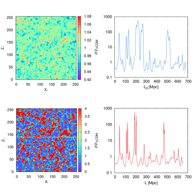
The Simsilun simulation consists of 16,777,216 worldlines, which are evolved from to . The variance of the density filed, at the present day (), if averaged over the spheres of radius Mpc is . This value is lower than the parameter of the Millennium simulation, but comparable to the parameter evaluated over the MFiled smoothed with Mpc. The initial density distribution is presented in the upper left panel in Fig. 4. This panel shows a slice through the simulation with a plane of , i.e. out of cells, only cells with are presented. The lower left panel in Fig. 4 shows the density distribution at the present instant. Again, this is the density distribution across the cells with . It should be noted, that the distribution of cells is not the same as the actual distribution of matter. This is due to the fact that cells do not evolve uniformly. In the Millennium simulations each cell evolves in the same way, and at the present day each cell has the same size of 2.68 Mpc ( Mpc Mpc). Using this conversion (hence the name ), the present-day density profile along a slice of and (this line is also depicted in the lower right panel) is presented in the upper right panel in Fig. 4. However, the real profile along this line (the axis is named to distinguish between the Millennium’s and cells’ ) is presented in the lower right panel in Fig. 4. As seen, overdensities are in fact smaller and underdense regions are larger, compared to the grid (cell) representation. Thus, the real distribution of structures is not the same as the one presented in lower left panel in Fig. 4, which distorts the real picture (making overdense regions look larger and underdense regions look smaller).
4.2 Evolution of matter, dark energy and spatial curvature
We first start by generalising the standard cosmological parameters (, , and ) to include averages and time evolution. Dark matter and dark energy parameters are easily generalisably and are defined as (Buchert, 2008)
| (40) |
The average is the volume average over a domain , and is defined as
| (41) |
where is density within a given cell, and is a volume of a given cell, and its evolution follows from
| (42) |
thus, apart from solving the silent universe evolution equations (16)–(19), we also need to solve the above equation to obtain the evolution of volume of a given domain . Finally, the parameter is the volume average Hubble parameter and is defined as
| (43) |
Relations (40) provide us with a generalisation of the standard cosmological parameters and . Firstly, this definition includes averages (as opposed to homogeneous and isotropic FLRW quantities). Secondly, these parameters are allowed to evolve with time, as opposed to the usual definition, which defines these parameters at the present-day instant.
For FLRW models, the parameters and , constrain the spatial curvature
| (44) |
The above is true even if one generalises the FLRW cosmological parameters to evolve with time, where and follow the definition (40) with and being the FLRW density and expansion rate respectively. For the inhomogeneous universe, the above formula is not exact. To show this, we start with the Hamiltonian constraint, from which it follows that the spatial curvature is
| (45) |
after volume averaging the above becomes
| (46) |
and by comparing with the FLRW definition of the parameter we get
| (47) |
Finally, dividing eq. (46) by we arrive at
| (48) |
where
| (49) |
is the kinematic backreaction. Thus, for inhomogeneous system, does not specify the special curvature as it does in the FLRW case. However, in most cases the kinematic backreaction remains small (Buchert et al., 2006; Wiltshire, 2009; Duley et al., 2013; Buchert et al., 2013; Roukema et al., 2013; Bolejko, 2017b), and so provides a reasonable approximation for the spatial curvature . From the Simsilun simulation, at the present-day instant, for virialisation scenario 1 and 2, and for virialisation scenario 3.
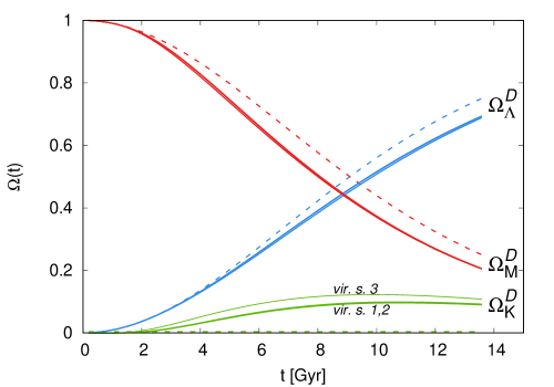
The evolution of the parameters , , and within the Simsilun simulation is presented in Fig. 5 (solid lines). The most striking results is that the spatial curvature is not zero but evolves. The Simsilun simulation starts with vanishing mean spatial curvature, but as the universe evolves the spatial curvature increases, and after Gyr it peaks at . After this instant, the spatial curvature starts to decrease. This turnaround is related to what is usually referred to as the cosmological “no-hair” conjecture. The cosmological “no-hair” conjecture states that the universe dominated by dark energy asymptotically approaches a homogeneous and isotropic de Sitter state (Wald, 1983; Pacher & Stein-Schabes, 1991). Thus, when dark energy becomes dominant the evolution of the spatial curvature plateaus and eventually decreases. There is a slight difference in between the virialisation scenarios 1, 2 and the virialisation scenario 3. There reason why virialisation scenario 3 leads to a more negative spatial curvature is due to the fact that the stable halo scenario assumes vanishing shear . As seen from eq. (45), contributes to the spatial curvature. Thus, neglecting shear within the virialisation scenario 3, means that virialised regions do not positively contribute to the spatial curvature and therefore the overall average curvature is more negative.
The emergence of the spatial curvature is consistent with findings of Roy et al. (2011) who studied the global gravitational instability of the FLRW models and showed that even tiny perturbations in result in a non-Friedmannian evolution of the spatial curvature. In the FLRW limit , so , where is the scale factor and is the curvature index. If then the even if initially then does not stay zero (as in the FLRW models) but evolves. The results presented in Fig. 5 confirm these findings.
The emergence of the spatial curvature is in contrast with the evolution of the universe modelled using N-body Newtonian simulations with periodic boundary conditions imposed. Within the comoving gauge (see below for a discussion on the gauge dependence), the nature of Newtonian interactions combined with the periodic boundary conditions (PBC) imply (Buchert & Ehlers, 1997; Kaiser, 2017; Buchert, 2017; Roukema, 2017)
In addition, the Newtonian N-body simulations often assume that the global evolution follows the Friedmann equations, consequently both and follow the Friedmann solution, which implies via (46)
Thus, within N-body Newtonian simulations the spatial curvature remains flat throughout the cosmic evolution.
The emergence of the spatial curvature is associated with the change of the evolution of other cosmological parameters as presented in Fig. 5. Since , thus the increase of the spatial curvature by results in similar decrease of the sum of and . For the Simsilun simulation this change is almost equally spread across these parameters and their amplitudes are smaller by compared to the CDM model (dashed lines) of the Millennium simulation (i.e. , at the present-day instant). There is a slight difference between the values of the parameters and depending on the assumed virialisation scenario, but this difference is small and is not visible in Fig. 5.
The results reported in this Section and presented in Fig. 5 were obtained within the comoving gauge. It has been a debate whether these findings are subject to a choice of a gauge. The parameters , , and are evaluated via averaging over domains of constant time, and so are susceptible to a choice of slicing and therefore could be gauge dependent. Recent results obtained by Adamek et al. (2015, 2017) showed that in the Poison gauge the backreaction (i.e. the change of the global evolution of the universe, for example as measured by the parameters , , and ) is negligible small, while in the comoving gauge (as in this paper) the backreaction can be large.
While it is not surprising that one can choose such a slicing where the backreaction vanishes, the question remains, which gauge is the most appropriate for studying the properties of the universe. Ultimately, the solution to this problem will be provided by ray tracing and evaluating cosmological observables in a gauge invariant way. However, it is interesting to notice that recent measurements of matter density based on weak leaning (DES) in the low-redshift universe show (DES Collaboration et al., 2017) which is lower than the CMB preferred value of (Planck Collaboration et al., 2016). Similarly, supernova observations (JLA) alone suggest lower values: and with very large uncertainties. It is only when these measurements are combined with high precision (i.e. small uncertainty) CMB data that they shift toward higher values: the DES data when combined with the Planck, SDSS, 6dF, BOSS, and JLA constraints push the matter density from to ; and the JLA supernova data when combined with CMB and BAO shift the matter density and cosmological constant to and .
While measurements of matter density at low redshift are subject to number of systematics, and may not directly correspond to , the results of the Simsilun simulation suggest that there should be a discrepancy between high and low redshift measurements. To theoretically estimate this discrepancy to high confidence one needs to develop ray tracing codes and evaluate observables in a gauge independent way. To empirically measure these discrepancies one requires high precision and high accuracy measurements free of any major systematics both at low and high redshifts.
5 Conclusions
This paper presents the results obtained from the code SIMplified SILent UNiverse (simsilun). The code solves the Einstein equations under the approximation of the ‘silent universe’ and evaluates the evolution of a cosmological system based on 4 scalars: density , expansion , shear , and Weyl curvature . In addition the code simsilun simplifies the procedure for setting up the initial conditions (hence the name ‘Simplified Silent Universe’), and allows to set up the model using only the initial density contrast. In this paper the initial conditions were set using the Millennium simulation, which provided a coherent set of initial conditions together with realistically appearing cosmic structures (cf. Fig. 4).
The simulation obtained this way, referred to as the Simsilun simulation, was employed to study the evolution of cosmological properties , (cf. eqs. (40)) and (cf. eq. (47)). Compared to the CDM model (i.e. the background model of the Millennium simulation) the spatial curvature is not flat but evolves from spatial flatness of the early universe to at the present-day instant (see Fig. 5). The emergence of the spatial curvature is associated with both and being smaller by approximately compared to the CDM model (note that in the CDM model we have , whereas for the Simsilun simulation ).
The code simsilun is publicly available via the Bitbucket repository666https://bitbucket.org/bolejko/simsilun and is distributed under the terms of the GNU General Public License. The code can easily be modified to include further effects, such as light propagation (Räsänen, 2010; Bolejko, 2011; Clarkson et al., 2012; Bolejko & Ferreira, 2012; Troxel et al., 2014; Peel et al., 2014), modelling of inhomogeneous non-symmetrical cosmic structures (Bolejko, 2006, 2007; Ishak & Peel, 2012; Peel et al., 2012; Sussman & Delgado Gaspar, 2015; Sussman et al., 2016), and the impact of the local cosmological environment on astronomical observations (Bolejko et al., 2016).
The evolution of the silent universe upon which the code is based is subject to several approximations and limitations. The silent approximation assumes vanishing pressure gradients, vanishing rotation, and vanishing magnetic part of the Weyl tensor. These assumptions are valid and preserved by linear and second order perturbations, but are expected to break down during a highly nonlinear stage of a collapse (Ellis & Tsagas, 2002). At this stage of the evolution also shell crossings start to develop and the fluid approximation is expected to break down. The code simsilun deals with this problem by forcing collapsing domains to virialise. Three different virialisation scenarios has been implemented and the results seems to be very weakly dependent on the choice of the virialisation mechanism. Finally, the results were obtained within the comoving gauge and therefore are subject to the limitations and applicability of the comoving coordinates (Adamek et al., 2015, 2017).
It seems that these limitations can only be properly addressed with full numerical relativistic cosmology. While the community is working towards such solutions, they are still not available yet (Bolejko & Korzyński, 2017) Comparison between different existing codes, such as the simsilun (this paper), gevolution (Adamek et al., 2016), and codes based on the BSSN formalism (Bentivegna & Bruni, 2016; Mertens et al., 2016; Macpherson et al., 2017) could provide insight into properties of relativistic systems such as our universe.
References
- Adamek et al. (2013) Adamek J., Daverio D., Durrer R., Kunz M., 2013, Phys. Rev. D, 88, 103527 (arXiv:1308.6524)
- Adamek et al. (2014) Adamek J., Durrer R., Kunz M., 2014, Class. Quant. Grav., 31, 234006 (arXiv:1408.3352)
- Adamek et al. (2015) Adamek J., Clarkson C., Durrer R., Kunz M., 2015, Physical Review Letters, 114, 051302 (arXiv:1408.2741)
- Adamek et al. (2016) Adamek J., Daverio D., Durrer R., Kunz M., 2016, J. Cosmol. Astropart. Phys., 7, 053 (arXiv:1604.06065)
- Adamek et al. (2017) Adamek J., Clarkson C., Daverio D., Durrer R., Kunz M., 2017, preprint, (arXiv:1706.09309)
- Alles et al. (2015) Alles A., Buchert T., Al Roumi F., Wiegand A., 2015, Phys. Rev. D, 92, 023512 (arXiv:1503.02566)
- Baldauf et al. (2015a) Baldauf T., Mercolli L., Mirbabayi M., Pajer E., 2015a, J. Cosmol. Astropart. Phys., 5, 007 (arXiv:1406.4135)
- Baldauf et al. (2015b) Baldauf T., Mercolli L., Zaldarriaga M., 2015b, Phys. Rev. D, 92, 123007 (arXiv:1507.02256)
- Bardeen (1980) Bardeen J. M., 1980, Phys. Rev. D, 22, 1882
- Baumann et al. (2012) Baumann D., Nicolis A., Senatore L., Zaldarriaga M., 2012, JCAP, 1207, 051 (arXiv:1004.2488)
- Baumgarte & Shapiro (1999) Baumgarte T. W., Shapiro S. L., 1999, Phys. Rev. D, 59, 024007 (arXiv:gr-qc/9810065)
- Bentivegna & Bruni (2016) Bentivegna E., Bruni M., 2016, Phys. Rev. Lett., 116, 251302 (arXiv:1511.05124)
- Blas et al. (2016) Blas D., Garny M., Ivanov M. M., Sibiryakov S., 2016, J. Cosmol. Astropart. Phys., 7, 052 (arXiv:1512.05807)
- Bolejko (2006) Bolejko K., 2006, Phys. Rev. D, 73, 123508 (arXiv:astro-ph/0604490)
- Bolejko (2007) Bolejko K., 2007, Phys. Rev. D, 75, 043508 (arXiv:astro-ph/0610292)
- Bolejko (2011) Bolejko K., 2011, Mon. Not. R. Astron. Soc., 412, 1937 (arXiv:1011.3876)
- Bolejko (2017a) Bolejko K., 2017a, preprint, (arXiv:1707.01800)
- Bolejko (2017b) Bolejko K., 2017b, J. Cosmol. Astropart. Phys., 6, 025 (arXiv:1704.02810)
- Bolejko & Ferreira (2012) Bolejko K., Ferreira P. G., 2012, J. Cosmol. Astropart. Phys., 5, 003 (arXiv:1204.0909)
- Bolejko & Korzyński (2017) Bolejko K., Korzyński M., 2017, International Journal of Modern Physics D, 26, 1730011 (arXiv:1612.08222)
- Bolejko & Lasky (2008) Bolejko K., Lasky P. D., 2008, Mon. Not. R. Astron. Soc., 391, L59 (arXiv:0809.0334)
- Bolejko et al. (2009) Bolejko K., Krasiński A., Hellaby C., Célérier M.-N., 2009, Structures in the Universe by Exact Methods: Formation, Evolution, Interactions. Cambridge University Press
- Bolejko et al. (2011) Bolejko K., Celerier M.-N., Krasinski A., 2011, Class. Quant. Grav., 28, 164002 (arXiv:1102.1449)
- Bolejko et al. (2016) Bolejko K., Nazer M. A., Wiltshire D. L., 2016, J. Cosmol. Astropart. Phys., 6, 035 (arXiv:1512.07364)
- Bondi (1947) Bondi H., 1947, Mon. Not. R. Astron. Soc., 107, 410
- Boylan-Kolchin et al. (2009) Boylan-Kolchin M., Springel V., White S. D. M., Jenkins A., Lemson G., 2009, Mon. Not. Roy. Astron. Soc., 398, 1150 (arXiv:0903.3041)
- Bruni et al. (1995) Bruni M., Matarrese S., Pantano O., 1995, Astroph. J., 445, 958 (arXiv:astro-ph/9406068)
- Buchert (2008) Buchert T., 2008, Gen. Rel. Grav., 40, 467 (arXiv:0707.2153)
- Buchert (2017) Buchert T., 2017, preprint, (arXiv:1704.00703)
- Buchert & Carfora (2008) Buchert T., Carfora M., 2008, Classical and Quantum Gravity, 25, 195001 (arXiv:0803.1401)
- Buchert & Ehlers (1997) Buchert T., Ehlers J., 1997, Astron. Astroph., 320, 1 (arXiv:astro-ph/9510056)
- Buchert & Ostermann (2012) Buchert T., Ostermann M., 2012, Phys. Rev. D, 86, 023520 (arXiv:1203.6263)
- Buchert et al. (2006) Buchert T., Larena J., Alimi J.-M., 2006, Classical and Quantum Gravity, 23, 6379 (arXiv:gr-qc/0606020)
- Buchert et al. (2009) Buchert T., Ellis G. F. R., van Elst H., 2009, Gen. Rel. Grav., 41, 2017 (arXiv:0906.0134)
- Buchert et al. (2013) Buchert T., Nayet C., Wiegand A., 2013, Phys. Rev. D, 87, 123503 (arXiv:1303.6193)
- Clarkson et al. (2009) Clarkson C., Ananda K., Larena J., 2009, Phys. Rev. D, 80, 083525 (arXiv:0907.3377)
- Clarkson et al. (2012) Clarkson C., Ellis G. F. R., Faltenbacher A., Maartens R., Umeh O., Uzan J.-P., 2012, Mon. Not. R. Astron. Soc., 426, 1121 (arXiv:1109.2484)
- DES Collaboration et al. (2017) DES Collaboration et al., 2017, preprint, (arXiv:1708.01530)
- Duley et al. (2013) Duley J. A. G., Nazer M. A., Wiltshire D. L., 2013, Classical and Quantum Gravity, 30, 175006 (arXiv:1306.3208)
- Ehlers (1993) Ehlers J., 1993, General Relativity and Gravitation, 25, 1225
- Einstein (1917) Einstein A., 1917, Sitzungsberichte der Königlich Preußischen Akademie der Wissenschaften (Berlin), p. 142
- Einstein & de Sitter (1932) Einstein A., de Sitter W., 1932, Proceedings of the National Academy of Science, 18, 213
- Ellis (1967) Ellis G. F. R., 1967, Journal of Mathematical Physics, 8, 1171
- Ellis (1971) Ellis G. F. R., 1971, in Sachs R. K., ed., General Relativity and Cosmology. pp 104–182
- Ellis (2009) Ellis G. F. R., 2009, General Relativity and Gravitation, 41, 581
- Ellis & Bruni (1989) Ellis G. F. R., Bruni M., 1989, Phys. Rev. D, 40, 1804
- Ellis & Buchert (2005) Ellis G. F. R., Buchert T., 2005, Physics Letters A, 347, 38 (arXiv:gr-qc/0506106)
- Ellis & MacCallum (1969) Ellis G. F. R., MacCallum M. A. H., 1969, Communications in Mathematical Physics, 12, 108
- Ellis & Tsagas (2002) Ellis G. F. R., Tsagas C. G., 2002, Phys. Rev. D, 66, 124015 (arXiv:astro-ph/0209143)
- Friedmann (1922) Friedmann A., 1922, Zeitschrift für Physik, 10, 377
- Friedmann (1924) Friedmann A., 1924, Zeitschrift für Physik, 21, 326
- Gierzkiewicz & Golda (2016) Gierzkiewicz A., Golda Z. A., 2016, Journal of Nonlinear Mathematical Physics, 23, 494
- Guo et al. (2013) Guo Q., White S., Angulo R. E., Henriques B., Lemson G., Boylan-Kolchin M., Thomas P., Short C., 2013, Mon. Not. Roy. Astron. Soc., 428, 1351 (arXiv:1206.0052)
- Hellaby (1996) Hellaby C., 1996, Classical and Quantum Gravity, 13, 2537
- Hellaby & Krasiński (2002) Hellaby C., Krasiński A., 2002, Phys. Rev. D, 66, 084011 (arXiv:gr-qc/0206052)
- Ishak & Peel (2012) Ishak M., Peel A., 2012, Phys. Rev. D, 85, 083502 (arXiv:1104.2590)
- Jenkins et al. (2001) Jenkins A., Frenk C. S., White S. D. M., Colberg J. M., Cole S., Evrard A. E., Couchman H. M. P., Yoshida N., 2001, Mon. Not. R. Astron. Soc., 321, 372 (arXiv:astro-ph/0005260)
- Kaiser (2017) Kaiser N., 2017, Mon. Not. R. Astron. Soc., 469, 744 (arXiv:1703.08809)
- Kasai (1995) Kasai M., 1995, Phys. Rev. D, 52, 5605
- Krasinski (1997) Krasinski A., 1997, Inhomogeneous Cosmological Models. Cambridge University Press
- Laigle et al. (2015) Laigle C., et al., 2015, Mon. Not. R. Astron. Soc., 446, 2744 (arXiv:1310.3801)
- Lemaître (1927) Lemaître G., 1927, Annales de la Société Scientifique de Bruxelles, 47, 49
- Lemaître (1933) Lemaître A. G., 1933, Annales de la Société Scientifique de Bruxelles, 53
- Lemson & Virgo Consortium (2006) Lemson G., Virgo Consortium t., 2006, ArXiv Astrophysics e-prints, (arXiv:astro-ph/0608019)
- Löffler et al. (2012) Löffler F., et al., 2012, Classical and Quantum Gravity, 29, 115001 (arXiv:1111.3344)
- Maartens et al. (1997) Maartens R., Lesame W. M., Ellis G. F. R., 1997, Phys. Rev. D, 55, 5219 (arXiv:gr-qc/9703080)
- Macpherson et al. (2017) Macpherson H. J., Lasky P. D., Price D. J., 2017, Phys. Rev. D, 95, 064028 (arXiv:1611.05447)
- Mertens et al. (2016) Mertens J. B., Giblin J. T., Starkman G. D., 2016, Phys. Rev. D, 93, 124059 (arXiv:1511.01106)
- Morita et al. (1998) Morita M., Nakamura K., Kasai M., 1998, Phys. Rev. D, 57, 6094 (arXiv:astro-ph/9711026)
- Navarro et al. (1996) Navarro J. F., Frenk C. S., White S. D. M., 1996, Astroph. J., 462, 563 (arXiv:astro-ph/9508025)
- Ostrowski et al. (2016) Ostrowski J. J., Buchert T., Roukema B. F., 2016, preprint, (arXiv:1602.00302)
- Ostrowski et al. (2017) Ostrowski J. J., Buchert T., Roukema B. F., 2017, Acta Polytechnica B, Proceedings Supplement, 10, 407 (arXiv:1703.04189)
- Pacher & Stein-Schabes (1991) Pacher T., Stein-Schabes J. A., 1991, Annalen der Physik, 503, 518
- Peebles (1980) Peebles P. J. E., 1980, The large-scale structure of the universe. Princeton University Press
- Peel et al. (2012) Peel A., Ishak M., Troxel M. A., 2012, Phys. Rev. D, 86, 123508 (arXiv:1212.2298)
- Peel et al. (2014) Peel A., Troxel M. A., Ishak M., 2014, Phys. Rev. D, 90, 123536 (arXiv:1408.4390)
- Planck Collaboration et al. (2016) Planck Collaboration et al., 2016, Astron. Astroph., 594, A13 (arXiv:1502.01589)
- Plebański & Krasiński (2006) Plebański J., Krasiński A., 2006, An Introduction to General Relativity and Cosmology. Cambridge University Press
- Rácz et al. (2017) Rácz G., Dobos L., Beck R., Szapudi I., Csabai I., 2017, Mon. Not. R. Astron. Soc., 469, L1 (arXiv:1607.08797)
- Rampf & Buchert (2012) Rampf C., Buchert T., 2012, J. Cosmol. Astropart. Phys., 6, 021 (arXiv:1203.4260)
- Räsänen (2010) Räsänen S., 2010, J. Cosmol. Astropart. Phys., 3, 018 (arXiv:0912.3370)
- Robertson (1929) Robertson H. P., 1929, Proceedings of the National Academy of Science, 15, 822
- Robertson (1933) Robertson H. P., 1933, Reviews of Modern Physics, 5, 62
- Roukema (2017) Roukema B. F., 2017, preprint, (arXiv:1706.06179)
- Roukema et al. (2013) Roukema B. F., Ostrowski J. J., Buchert T., 2013, J. Cosmol. Astropart. Phys., 10, 043 (arXiv:1303.4444)
- Roy et al. (2011) Roy X., Buchert T., Carloni S., Obadia N., 2011, Classical and Quantum Gravity, 28, 165004 (arXiv:1103.1146)
- Shibata & Nakamura (1995) Shibata M., Nakamura T., 1995, Phys. Rev. D, 52, 5428
- Springel et al. (2005) Springel V., et al., 2005, Nature, 435, 629 (arXiv:astro-ph/0504097)
- Sussman (2013) Sussman R. A., 2013, Class. Quant. Grav., 30, 235001 (arXiv:1305.3683)
- Sussman & Bolejko (2012) Sussman R. A., Bolejko K., 2012, Classical and Quantum Gravity, 29, 065018 (arXiv:1109.1178)
- Sussman & Delgado Gaspar (2015) Sussman R. A., Delgado Gaspar I., 2015, Phys. Rev. D, 92, 083533 (arXiv:1508.03127)
- Sussman et al. (2016) Sussman R. A., Delgado Gaspar I., Hidalgo J. C., 2016, J. Cosmol. Astropart. Phys., 3, 012 (arXiv:1507.02306)
- Szafron (1977) Szafron D. A., 1977, J. Math. Phys., 18, 1673
- Szekeres (1975) Szekeres P., 1975, Commun. Math. Phys., 41, 55
- Tolman (1934) Tolman R. C., 1934, Proc. Natl. Acad. Sci. U.S.A., 20, 169
- Troxel et al. (2014) Troxel M. A., Ishak M., Peel A., 2014, J. Cosmol. Astropart. Phys., 3, 040 (arXiv:1311.5936)
- Tsagas et al. (2008) Tsagas C. G., Challinor A., Maartens R., 2008, Phys. Rep., 465, 61 (arXiv:0705.4397)
- Vogelsberger et al. (2014) Vogelsberger M., et al., 2014, Nature, 509, 177 (arXiv:1405.1418)
- Wald (1983) Wald R. M., 1983, Phys. Rev. D, 28, 2118
- Walker (1935) Walker A. G., 1935, The Quarterly Journal of Mathematics, 6, 81
- Wiltshire (2009) Wiltshire D. L., 2009, Phys. Rev. D, 80, 123512 (arXiv:0909.0749)
- de Sitter (1917) de Sitter W., 1917, Koninklijke Nederlandse Akademie van Wetenschappen Proceedings Series B Physical Sciences, 19, 1217
- van Elst & Ellis (1996) van Elst H., Ellis G. F. R., 1996, Classical and Quantum Gravity, 13, 1099 (arXiv:gr-qc/9510044)
- van Elst et al. (1997) van Elst H., Uggla C., Lesame W. M., Ellis G. F. R., Maartens R., 1997, Classical and Quantum Gravity, 14, 1151 (arXiv:gr-qc/9611002)