Gas structure and dynamics towards bipolar infrared bubble

Abstract

We present multi-wavelength analysis for four bipolar bubbles (G045.386-0.726, G049.998-0.125, G050.489+0.993, and G051.610-0.357) to probe the structure and dynamics of their surrounding gas. The ¹²CO $J$=1-0, ¹³CO $J$=1-0 and C¹⁸O $J$=1-0 observations are made with the Purple Mountain Observation (PMO) 13.7 m radio telescope. For the four bipolar bubbles, the bright 8.0 $\mu$m emission shows the bipolar structure. Each bipolar bubble is associated with an H II region. From CO observations we find that G045.386-0.726 is composed of two bubbles with different distances, not a bipolar bubble. Each of G049.998-0.125 and G051.610-0.357 is associated with a filament. The filaments in CO emission divide G049.998-0.125 and G051.610-0.357 into two lobes. We suggest that the exciting stars of both G049.998-0.125 and G051.610-0.357 form in a sheet-like structure clouds. Furthermore, G050.489+0.993 is associated with a clump, which shows a triangle-like shape with a steep integrated intensity gradient towards the two lobes of G050.489+0.993. We suggest that the two lobes of G050.489+0.993 have simultaneously expanded into the clump.

Keywords H II regions — ISM: bubbles — ISM: clouds

1 Introduction

Infrared bubbles are the bright 8.0 $\mu$m emission surrounding O and early-B stars. The bright 8 $\mu$m emission is attributed to polycyclic aromatic hydrocarbons (PAHs, Lèger & Puget, 1984). The PAHs molecules can be destroyed inside the ionized gas, but are excited in the photodissociation region (PDR) by the UV radiation within H II region (Pomarè s et al., 2009). H II regions are ionized by massive stars. The UV radiation of an H II region can excite its surrounding gas to create a bright mid-infrared bubble. So the bubbles are usually found in or near massive star-forming regions (see e.g., Deharveng et al., 2003; Xu & Ju, 2014a; Xu et al., 2014b). If bubble forms in a sheet-like molecular cloud, whose thickness is not greater than the bubble size, we will see a 2D ring bubble. And when the bubble size is less than the thickness of the molecular cloud, a 3D spherical-structure bubble will form. Hence, the environment of bubble formed may determine their morphology.

Table 1 : Physical parameters of H II regions and molecular gas associated with four bipolar bubbles

Name	R.A.	Decl.	S	$V_{\rm H}$	Distance	$N_{\rm Ly}^{c}$	Typed	$N(\rm H_{2}$)	$M(\rm H_{2}$)
	(J2000)	(J2000)	(mJy)	km $\rm s^{-1}$	(kpc)	(photons $\rm s^{-1}$)		(cm -2)	M⊙
G045.386-0.726	19h17m00.5s	10∘44′33′′	610	52.5	8.0	7.4$\times$1048	O6.5$\sim$O6	–	–
G049.998-0.125	19h23m46.1s	15∘04′54′′	410	38.5/73.2	4.7b	1.7$\times$1048	O8.5$\sim$O8	5.6$\times$1021	8.3$\times$103
G050.489+0.993	19h20m38.2s	16∘02′29′′	140a	57.1	5.4	6.4$\times$1047	$<$O9.5	3.1$\times$1021	4.4$\times$103
G051.610-0.357	19h27m48.0s	16∘23′25′′	270	41.1	5.3	1.4$\times$1048	O8.5$\sim$O8	3.6$\times$1021	3.7$\times$103

Bipolar bubble has a simple morphology, so it is easy to locate the ionized and neutral components in space. So far very few studies describe the formation and evolution of the bipolar bubble. Deharveng et al. (2010) used the ATLASGAL survey at 870 $\mu$m to study 102 bubbles detected by spitzer-GLIMPSE, 86$\%$ of which enclose classical H II region ionized by O and B stars. Only bubbles N39 and N52 show a bipolar morphology (Churchwell et al., 2006), which are associated with a filament. They considered that the ionized stars of their two bipolar bubbles formed in a massive and rather flat molecular cloud. Deharveng et al. (2015) identified and studied two bipolar bubbles. H II regions G319.88+00.79 and G010.32-00.15 are located at the centre of these two bipolar bubbles, respectively. Especially for H II regions G319.88+00.79, there is a filament that will divide the bipolar bubble into two ionized lobes. They concluded that the exciting stars of each bipolar H II region are formed in a sheet-like structure clouds. The sheet observed edge-on appears as a filament. According to Deharveng et al. (2010, 2015), the bipolar bubble forms when ionization front breaks through the two opposite faces of the sheet-like cloud simultaneously. Thus, the observation of bipolar bubbles can also provide important information on the structure of their surrounding cloud.

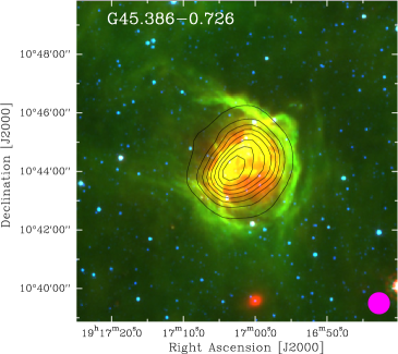
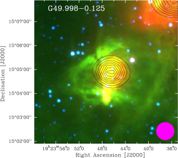
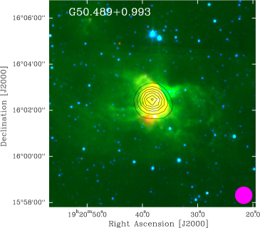
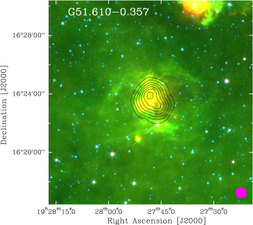
Fig. 1 : 1.4 GHz radio continuum contours in black colour, overlaid on the three color image of bipolar bubble composed from the Spitzer 4.5 $\mu$m (in blue), 8.0 $\mu$m (in green), and 24 $\mu$m (in red) bands. G045.386-0.726: The black contour levels are 3.5 (5$\sigma$), 14.0, 24.5, 35.0, 45.5, 56.0, 66.5, and 77.0 mJy beam^-1; G049.998-0.125: The black contour levels are 4.5 (5$\sigma$), 7.1, 9.8, 12.5, 15.1, 17.8, 20.5, and 23.2 mJy beam^-1; G050.489+0.993: The black contour levels are 3.1 (5$\sigma$), 6.1, 9.1, 12.2, 15.3, 18.3, and 21.4 mJy beam^-1; G051.610-0.357: The black contour levels are 2.8 (5$\sigma$), 4.5, 6.2, 7.8, 9.5, 11.2, and 12.9 mJy beam^-1.

According to the Green Bank Telescope (GBT) and Arecibo H II region discovery surveys, Anderson et al. (2011) and Bania et al. (2012) identified eleven bipolar bubbles. Considering the angular resolution of our used telescope (Purple Mountain Observation 13.7 m radio telescope), we only selected four bipolar bubbles, whose parameters are lised in Table 1, including the coordinates, the integrated flux densities, the hydrogen radio recombination line (RRL) velocities ($V_{\rm H}$), and the distances. In this paper, we performed a multi-wavelength study to the four bipolar bubbles to investigate the gas structure around H II regions. Our observations and data reduction are described in Sect.2, and the results are presented in Sect.3. In Sect.4, we discuss the gas structure around the four bipolar bubbles, while our conclusions are summarized in Sect.5.

2 Observations

2.1 Purple Mountain Data

We made the mapping observations for four bipolar bubbles and their adjacent regions in the transitions of ¹²CO $J$=1-0, ¹³CO $J$=1-0 and C¹⁸O $J$=1-0 lines using the Purple Mountain Observation (PMO) 13.7 m radio telescope at De Ling Ha in the west of China at an altitude of 3200 meters, during May 2015. The 3$\times$3 beam array receiver system in single-sideband (SSB) mode was used as front end. The back end is a fast Fourier transform spectrometer (FFTS) of 16384 channels with a bandwidth of 1 GHz, corresponding to a velocity resolution of 0.16 km s^-1 for ¹²CO $J$=1-0, and 0.17 km s^-1 for ¹³CO $J$=1-0 and C¹⁸O $J$=1-0. ¹²CO $J$=1-0 was observed at upper sideband, while ¹³CO $J$=1-0 and C¹⁸O $J$=1-0 were observed simultaneously at lower sideband. The half-power beam width (HPBW) was 53^′′ at 115 GHz and the main beam efficiency was 0.5. The pointing accuracy of the telescope was better than 5^′′, which was derived from continuum observations of planets (Venus, Jupiter, and Saturn). The source W51D (19.2 K) was observed once per hour as flux calibrator. Mapping observations used the on-the-fly mode. The standard chopper wheel calibration technique is used to measure antenna temperature $T_{\rm A}^{\ast}$ corrected for atmospheric absorption. The final data was recorded in brightness temperature scale of $T_{\rm mb}$ (K). The data were reduced using the GILDAS/CLASS package.

2.2 Archival Data

The 1.4 GHz radio continuum emission data were obtained from the NRAO VLA Sky Survey (NVSS), with a noise of about 0.45 mJy/beam and a resolution of 45^′′ (Condon et al., 1998); We extracted 870 $\mu$m data from the ATLASGAL survey (Schuller et al., 2009). The survey was carried out with the Large APEX Bolometer Camera observing at 870 $\mu$m (345 GHz). The APEX telescope has a full width at half-maximum (FWHM) beam size of 19^′′ at this frequency; We also utilized mid-infrared data in two bands (4.5 and 8.0 $\mu$m) from the Spitzer GLIMPSE survey and mid-infrared data in 24 $\mu$m band from the MIPSGAL survey (Benjamin et al., 2003; Rieke et al., 2004). The resolutions at 4.5 $\mu$m and 8.0 $\mu$m are $<$ $2.0^{\prime\prime}$, while the MIPSGAL resolution at 24 $\mu$m is 6^′′; We also retrieved the K (2.17 $\mu$m) band images from Two Micron All Sky Survey (2MASS)(Skrutskie et al., 2006).

3 Results

3.1 Infrared and Radio Continuum Images

Figure 1 shows composite three-color images of the four bipolar bubbles. The three infrared bands are the Spitzer 4.5 $\mu$m (in blue), 8.0 $\mu$m (in green), and 24 $\mu$m (in red). In Fig. 1, the PAH emission, traced by the bright 8 $\mu$m, delineates the structure for each bipolar bubble. Two lobes of both G050.489+0.993 and G051.610-0.357 are symmetrical, and thus they are the standard bipolar bubble. For G049.998-0.125, the left lobe is smaller than the right lobel. Compared with the other three bipolar bubble, G045.386-0.726 shows a complex sructure. The 24 $\mu$m emission traces heated small dust grains (Watson et al., 2008). The hot dust emission in Fig. 1 displays a dense structure between two lobes for each bipolar bubble. The NVSS 1.4 GHz radio continuum emission, which can be used to trace ionized gas, is also overlaid in Fig. 1 in black contours. In Fig. 1, the ionized gas emission are spatially coincident with the hot dust emission observed at the 24 $\mu$m (red color). For each bipolar bubble, both the ionized gas and hot dust emission show a single structure, suggesting that each bipolar bubble is created by an H II region, not adjacent bubbles surrounding distince H II regions.

To estimate the ionized star types of these H II regions, we will calculate the ionizing luminosity. Assuming the radio continuum emission is optically thin, the ionizing luminosity $N_{\rm Ly}$ is computed by Mezger et al. (1974)

$$\mathit{N_{\rm Ly}}=4.76\times 10^{48}(\frac{\nu}{\rm GHz})^{0.1}(\frac{T_{e}}{\rm K})^{-0.45}(\frac{S_{\nu}}{\rm Jy})(\frac{D}{\rm kpc})^{2}\rm~{}s^{-1},$$ (1)

Where $\nu$ is the frequency, $T_{e}$ is the effective electron temperature, $S_{\nu}$ is the observed specific flux density, and $D$ is the distance to H II region. Anderson et al. (2011) measured the flux densities of H II regions G045.386-0.726, G049.998-0.125, and G051.610-0.357 at 9 GHz. For the H II region related to G050.489+0.993, we measure its flux density at 1.4 GHz. Moreover, we adopt an effective electron temperature of 10⁴ K. Inoue (2001) suggested that only half of Lyman continuum photons from the central source in a Galactic H II region ionizes neutral hydrogen, the remainder being absorbed by dust grains within the ionized region. Finally, we obtain the ionizing luminosity$N_{\rm Ly}$. According to Martins et al. (2005), the spectral type of the ionizing star for each H II region is derived, which are lised in Table 1.

Figure 2 (left panels) only shows the K frames overlaid with 1.4 GHz continuum emission for three bipolar bubbles (G049.998-0.125, G050.489+0.993, and G051.610-0.357). G045.386-0.726 is not a real bipolar bubble (see Sec.3.2.1). To further look for the ionized star types of these H II regions, we use the 2MASS All-Sky Point source database in the near-infrared J(1.25 $\mu$m), H(1.65 $\mu$m) and K(2.17 $\mu$m) bands, with a signal-to-noise ratio (S/N) greater than 10. Because the 1.4 GHz radio continuum emission can trace the ionized gas of each bipolar bubble, the ionized stars are only located within the 1.4 GHz radio continuum emission regions. Using the database, we select near-infrared sources, and distribute these sources over the K band images. Figure 2 (right panels) shows the (H) versus (H–K) color-color (CC) diagrams. Table 1 gives that the ionized star types of both G049.998-0.125 and G051.610-0.357 are between O8.5V and O8V. From Fig. 2, we see that two near-infrared sources are located between O8.5V and O8V for G049.998-0.125, and three near-infrared sources near and between O8.5V and O8V for G051.610-0.357. In Fig. 2 (left panels), the red circles mark the positions of these selected near-infrared sources. Generally, the ionized stars are located near or on the peak position of the ionized gas emission. From Fig. 2 (left panels), we suggest that #1 and #2 may be the ionized stars of G049.998-0.125, and #2 is likely to be the ionized star of G051.610-0.357. For G050.489+0.993, the type of its ionized star is greater than O9.5V. Several near-infrared sources are below the 09.5V line, as shown in Fig. 2 (right panels) for G050.489+0.99, but we see that three bright near-infrared sources are located near the peak postion of the ionized gas. Comparing the CC diagram, #1 may be the ionized stars of G050.489+0.993.

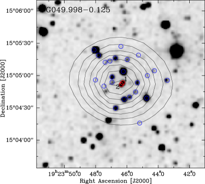
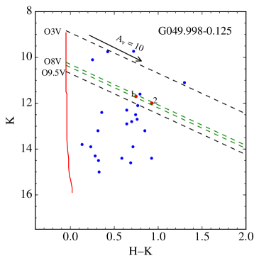
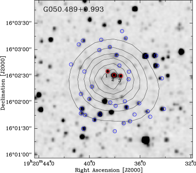
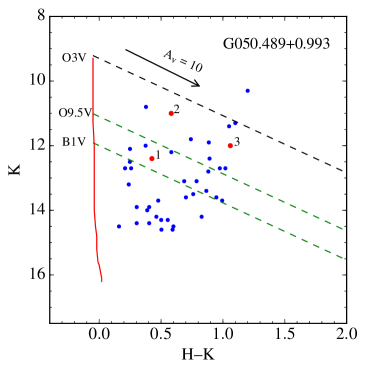
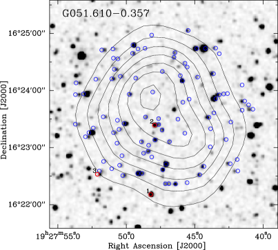
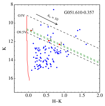
Fig. 2 : Left panels: Radio continuum emission at 1.4 GHz superimposed on the K frame of each H II region. The blue circles represent the selected near-infrared sources, while the red circles may indicate the ionized stars. Left panels: K versus H–K diagram for sources detected in all the three 2MASS bands. The main sequence is also drawn for different distances (red lines). The slanting dashed lines trace the reddening vectors for each spectral type (extinction law of Rieke & Lebofsky (1985)). While the slanting green dashed lines represent the positions of O8.5V and O8V, respectively.

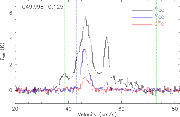
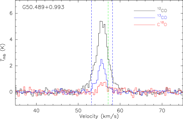
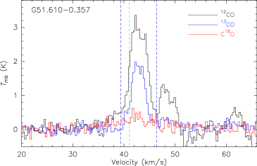
Fig. 3 : ¹²CO $J$=1-0, ¹³CO $J$=1-0, and C¹⁸O $J$=1-0 spectra over the observed region ($>$3$\sigma$) for each bipolar bubbles. The green dashed lines indicate the RRL velocity of each H II region, while dubble blue and red lines mark the integrated velocity ranges.

3.2 Dust and CO Molecular Emission

CO observation can reveal whether molecular gas is associated with bipolar bubble along our line of sight. To check the morphology of molecular gas consistent with each bipolar bubble, we use ¹²CO $J$=1-0, ¹³CO $J$=1-0, and C¹⁸O $J$=1-0 lines to trace the molecular gas emision, and use 870 $\mu$m continuum to trace cool dust emission.

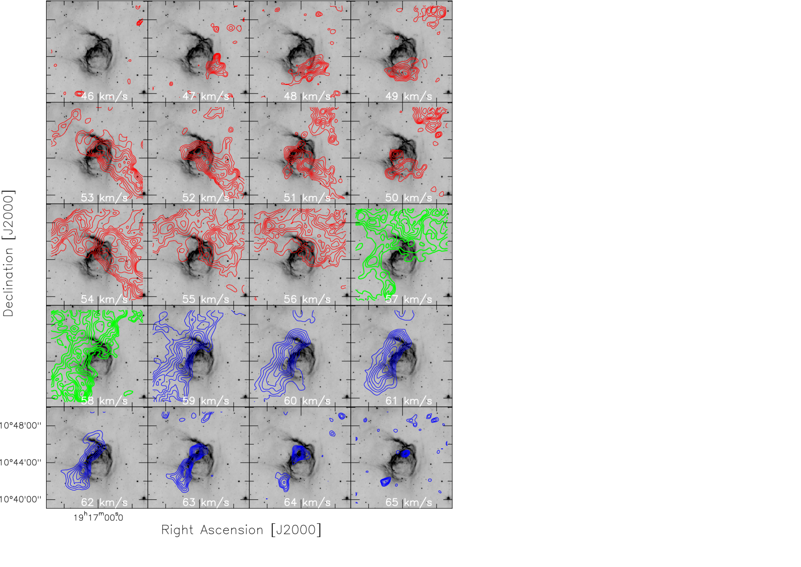
Fig. 4 : ¹³CO $J$=1-0 channel maps of G045.386-0.726 in step of 1 km s^-1 overlaid on the Spitzer-IRAC 8 $\mu$m emission (grey). Central velocities are indicated in each image. The different gas components are marked by different color contours.

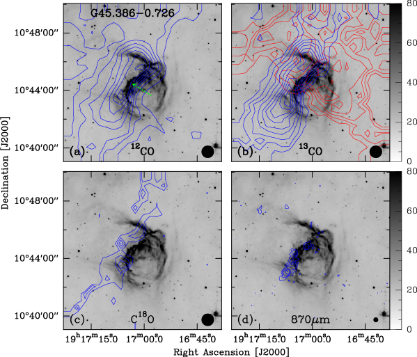
Fig. 5 : G045.386-0.726. The integrated intensity maps in CO lines and 870 $\mu$m map are superimposed on the Spitzer 8.0 $\mu$m map (grey scale). (a) panel: The blue contour levels are from 19.5 (3$\sigma$) to 55.9 by a step of 5.2 K km s^-1, and the integrated velocity is from 57.0 to 65.5 km s^-1. (b): The blue contour levels are from 5.4 (3$\sigma$) to 16.9 by a step of 1.4 K km s^-1, while the blue contour levels are from 5.4 (3$\sigma$) to 12.6 by a step of 1.8 K km s^-1. For red contours, the integrated velocity is from 47.0 to 57.0 km s^-1. (c) panel: The blue contour levels are from 2.1 (3$\sigma$) to 3.8 by a step of 0.6 K km s^-1. (d) panel: The blue contour levels are from 0.2 (3$\sigma$) to 0.6 by a step of 0.1 Jy/beam.

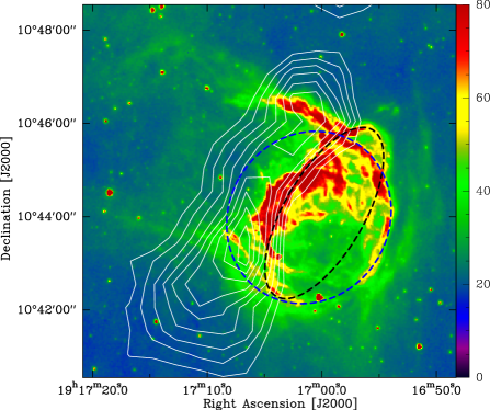
Fig. 6 : ¹³CO $J$=1-0 integrated intensity map (white contours) overlaid on the Spitzer 8.0 $\mu$m map (color scale). The range of integrated velocity is from 57.0 to 65.0 ${\rm km~{}s}^{-1}$

. The two elliptical dashed circles represent two bubbles.

3.2.1 G045.386-0.726

Bipolar bubble G045.386-0.726 is associated with a compact H II region and bubble N95 (Deharveng et al., 2010). The H II region has a hydrogen radio recombination line (RRL) velocity of 52.5 ${\rm km~{}s}^{-1}$ (Anderson et al., 2011). From Fig. 3, we see that there are multiple gas components in the G045.386-0.726 region. Comparing the optically thick ¹²CO line, the ¹³CO line is more suited to trace relatively dense gas ($\sim$10³ cm^-3). Using channel maps (Fig. 4) of ¹³CO line, we found two gas components, which may coindcient with G045.386-0.726 in space. One component is located between 47.0 and 58.0 ${\rm km~{}s}^{-1}$ (red+green countours), while the other component is in interval 57.0 to 65.0 ${\rm km~{}s}^{-1}$ (green+blue contours). The ¹³CO emission (green contours) between 57.0 and 58.0 ${\rm km~{}s}^{-1}$ shows that above two components may connect in the velocity and space. We use these two velocity ranges to make the integrated intensity maps, as shown in Fig. 5. The ¹²CO, ¹³CO, and C¹⁸O emission in interval 57.0 to 65.0 ${\rm km~{}s}^{-1}$, which is correlated with the 870 $\mu$m emission, show a filamentary structure from northwest to southeast. The filament displays an arc-like structure with a steep integrated intensity gradient, whose direction (green arrow) is perpendicular to the filament. The arc-like structure just encloses the bipolar bubble G045.386-0.726. Moreover, the CO emission in interval 47.0 to 58 ${\rm km~{}s}^{-1}$, which exhibits a diffuse structure, is distribute mainly over the northwest of G045.386-0.726. The RRL velocity of H II region associated with the bipolar bubble G045.386-0.726 is 52.5 ${\rm km~{}s}^{-1}$, indicating that the diffuse CO emission (red contours) is related to bipolar bubble G045.386-0.726, while the filament may be associated with the other bubble. We use two bubbles to fit the Spitzer 8.0 $\mu$m image, as shown in Fig. 6. Hence, we conclude that these two bubbles with different distances overlap along our sight of line, and thus making it look like a bipolar bubble. Therefore, we will not further analyse G045.386-0.726 in the rest of the text, except for the discussion section.

Fig. 7 : G049.998-0.125. The integrated intensity maps in CO lines and 870 $\mu$m map are superimposed on the Spitzer 8.0 $\mu$m map (grey scale). (a) panel: The blue contour levels are from 12.0 (3$\sigma$) to 48.0 by a step of 4.0 K km s^-1. (b) panel: The blue contour levels are from 4.5 (3$\sigma$) to 23.4 by a step of 2.7 K km s^-1. (c) panel: The blue contour levels are from 2.4 (3$\sigma$) to 4.8 by a step of 0.5 K km s^-1. (d) panel: The blue contour levels are from 0.2 (3$\sigma$) to 0.8 by a step of 0.1 Jy/beam. The pluses mark the position of the dust clumps.

3.2.2 G049.998-0.125

Bipolar bubble G049.998-0.125 is correlated with a compact H II region. Anderson et al. (2011) gave that this H II region has two RRL velocities, which are 38.5 ${\rm km~{}s}^{-1}$ and 73.2 ${\rm km~{}s}^{-1}$. Through the channel maps of ¹³CO line, we inspect gas component for our studied region, and find that the component in interval 43.2 to 50.0 ${\rm km~{}s}^{-1}$ is associated with G049.998-0.125 in morphology. The two RRL velocities for G049.998-0.125 are not located between 43.2 and 50.0 ${\rm km~{}s}^{-1}$. Using the velocity range of 43.2 to 50.0 ${\rm km~{}s}^{-1}$, we made the integrated intensity maps (Fig. 7). The ¹²CO, ¹³CO, and C¹⁸O emission show a filamentary structure from north to south, but our observations did not resolve the bipolar structure of G049.998-0.125. Comparing the CO emission, 870 $\mu$m emission also displays the filamentary structure with two dense clumps. Based on the ATLASGAL clump survey (Csengeri et al., 2014), one clump is G049.9996-0.1296, the other clump is G049.9842-0.1364. The masses of the ATLASGAL clumps were determined using the relation

$$\mathit{M_{\rm clump}}=\frac{S_{870}D^{2}}{\kappa_{870}B_{870}(T_{d})}$$ (2)

where $S_{870}$ is the flux density at the frequency 870 $\mu$m and $D$ is the distance to the clumps. $\kappa_{870}$ is the dust opacity, which is adopted as 1.0 cm² g^-1 (Ossenkopf & Henning, 1994). Here the ratio of gas to dust was taken as 100. $B_{870}(T_{\rm d})$ is the Planck function for the dust temperature $T_{d}$ and frequency 870 $\mu$m. Deharveng et al. (2015) indicated that the mean temperature of the clumps adjacent to the ionized region is about 20 K. Here, we also used a dust temperature of about 20 K for each ATLASGAL clump. The obtained parameters are listed in Table 2. To determine whether the two ATLASGAL clumps have sufficient mass to form massive stars, we must consider their sizes and masses. According to Kauffmann & Pillai (2010), if the clump mass is $M(r)\geq 580M_{\odot}(r/pc)^{1.33}$, then they can potentially form massive stars. We find that both the two ATLASGAL clumps lie above the threshold, indicating that the ATLASGAL clumps are dense and massive enough to potentially form massive stars. Furthermore, the filament in 870 $\mu$m is perpendicular to G049.998-0.125, and divides G049.998-0.125 into two lobes. The systemic velocity of the filament is 47.0 km s^-1, which is measured from Fig. 3. Based on the Bayesian Distance Calculator (Reid et al., 2016), we obtain that the distance of the filament and G049.998-0.125 is 4.7 kpc.

3.2.3 G050.489+0.993

G050.489+0.993 is a textbook example of bipolar bubble. An H II region is located on the center of G050.489+0.993, whose RRL velocity is 57.1 ${\rm km~{}s}^{-1}$. From Fig. 3, we note that there is a single component in this region. The RRL velocity of G045.386-0.726 is just located between 53.1 and 58.1 ${\rm km~{}s}^{-1}$. Hence, the molecular gas in interval 53.1 to 58.1 ${\rm km~{}s}^{-1}$ is associated with G050.489+0.993. We made the integrated intensity maps, which is shown in Fig. 8. Both ¹²CO and ¹³CO emission in Fig. 8 displays a large clump, while the C¹⁸O and 870 $\mu$m emission are relatively weak. Moreover, the ¹³CO emission of the clump presents a triangle-like shape, and has an integrated intensity gradient toward the direction of two lobes of G050.489+0.993, which are marked in two green arrows. It suggests that the shocks from G050.489+0.993 have expanded into the clump, and have compressed it. The clump consistent with IRDC G38.95-0.47 also shows the same shape (Xu et al., 2013), but it is created by different H II regions G38.91-0.44 and G39.30-1.04.

Table 2 : Properties clumps around the bipolar bubble G049.998-0.125

Name	R.A.	Decl.	$\rm\theta_{maj}\times\rm\theta_{min}$	$R_{\rm eff}^{\rm a}$	S	M($\rm H_{2}$)
	(J2000)	(J2000)	${}^{\prime\prime}\times^{\prime\prime}$	(pc)	(Jy)	M⊙
G049.9996-0.1296	19h23m47.40s	15∘04′50.8′′	34$\times$19	0.29	1.4	314.1
G049.9842-0.1364	19h23m47.04s	15∘03′50.4′′	42$\times$23	0.35	2.0	448.8

3.2.4 G051.610-0.357

Bipolar bubble G045.386-0.726 is also associated with a compact H II region. This H II region has a hydrogen RRL velocity of 41.1 ${\rm km~{}s}^{-1}$. From Fig. 3, we see that ¹²CO spectrum shows multiple components, while ¹³CO spectrum exhibits a single component, which is located between 39.1 and 46.1 ${\rm km~{}s}^{-1}$. The integrated intensity maps are shown in Fig. 9. The ¹²CO and ¹³CO emission show a filamentary structure from northwest to southeast. The filament is just perpendicular to G049.998-0.125, and divides G049.998-0.125 into two lobes. Possiblely the C¹⁸O and 870 $\mu$m emission is weaker in this region, here we only detect a little emisson for C¹⁸O and 870 $\mu$m.

Fig. 8 : G050.489+0.993. The integrated intensity maps in CO lines and 870 $\mu$m map are superimposed on the Spitzer 8.0 $\mu$m map (grey scale)(a) panel: The blue contour levels are from 7.5 (3$\sigma$) to 37.5 by a step of 5.0 K km s^-1. (b) panel: The blue contour levels are from 1.8 (3$\sigma$) to 12.3 by a step of 1.5 K km s^-1. (c) panel: The blue contour levels are from 0.9 (3$\sigma$) to 1.3 by a step of 0.1 K km s^-1. (d) panel: The blue contour level is 0.2 Jy/beam (3$\sigma$).

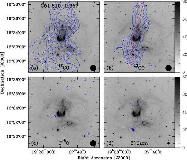
Fig. 9 : G051.610-0.357. The integrated intensity maps in CO lines and 870 $\mu$m map are superimposed on the Spitzer 8.0 $\mu$m map (grey scale)(a) panel: The blue contour levels are from 6.5 (3$\sigma$) to 22.1 by a step of 2.6 K km s^-1. (b) panel: The blue contour levels are from 1.5 (3$\sigma$) to 3.3 by a step of 0.3 K km s^-1.

3.2.5 Physical parameters

To estimate the column density and mass of the molecular gas around the three bipolar bubbles, we used the optical thin ¹³CO $J$=1-0 emission. Assuming local thermodynamical equilibrium (LTE), the column density was estimated via (Garden et al., 1991)

$$\mathit{N(\rm^{13}CO)}=4.71\times 10^{13}\frac{T_{\rm ex}+0.88}{\rm exp(-5.29/T_{\rm ex})}\int T_{\rm mb}dv~{}\rm cm^{-2},$$ (3)

where $T_{\rm ex}$ is the mean excitation temperature of the molecular gas, $T_{\rm mb}$ is the corrected main-beam temperature of ¹³CO $J$=1-0, and $dv$ is the velocity range.

The ¹²CO emission is optical thick, so we used ¹²CO to estimate $T_{\rm ex}$ via following the equation (Garden et al., 1991)

$$\mathit{T_{\rm ex}}=\frac{5.53}{{\ln[1+5.53/(T_{\rm mb}+0.82)]}},$$ (4)

where $T_{\rm mb}$ is the corrected main-beam brightness temperature of ¹²CO.

In addition, we used the relation $N(\rm H_{2})/\it N(\rm^{13}CO)$ $\approx$ $7\times 10^{5}$ (Castets et al., 1982) to estimate the H₂ column density. The mass of the molecular gas can be determined by

$$\mathit{M_{\rm H_{2}}}=\mu_{g}m(\rm H_{2})\it N(\rm H_{2})\it S,$$ (5)

where $\mu_{g}$=1.36 is the mean atomic weight of the gas, $m(\rm H_{2})$ is the mass of a hydrogen molecule, and $S$ is the projected 2D area of the ring. The obtained column density and mass of the molecular gas are listed in Table 1. From Table 1, we see that the parental molecular gas in coincidence with the three bipolar bubbles are the giant molecular cloud.

4 Discussion

From the CO observations, we suggest that there may be two bubbles with different distances overlap along our sight of line, and thus making G045.386-0.726 look like a bipolar bubble. Interestingly, in the velocity interval of 57.0 to 65.0 ${\rm km~{}s}^{-1}$, the ¹²CO, ¹³CO, and C¹⁸O emission are correlated with the 870 $\mu$m emission in shape, both of which show a filament. The filament displays an arc-like structure with a steep interated intensity gradient toward G045.386-0.726, implying that G045.386-0.726 is interacting with the filament. Recently, star formation are found along filaments, so many studies are devoted to filaments. As the suggestion of Deharveng et al. (2015), it is often forgotten that 2D gas sheets can be mistaken as filaments if we view edge-on.

From Fig. 6, we also note that the bright 8 $\mu$m emission marked by black dashed lines show a ring-like structure. Since the ring has an inclination angle with our line of sight, then it appears to display an elliptical structure. The existence of the inclination indicates that the ring is not a 3D spherically symmetrical, but a 2D ring. The filamentary molecular clouds are usually associated with massive star-forming regions (André et al., 2014). Once a massive star forms inside or near a filament, UV radiation and stellar winds will excite the surrounding gas and create an infrared bubble (Zhang et al., 2016). The main emission of the bubble is the bright PAHs. The PAHs molecules are easily excited by the UV radiation from H II region (Pomarè s et al., 2009). It means that a bright 8 $\mu$m bubble is created only if there should be some molecular gas adjacent to H II region, containing the collected gas from the expansion of H II region. If the bubble is a 2D ring, the interaction surface between the filament and the ring may be not greater than the thickness of the ring, indicating that the filament in Fig. 4 is a sheet with a thickness of a few parsecs rather than a cylindrical filament.

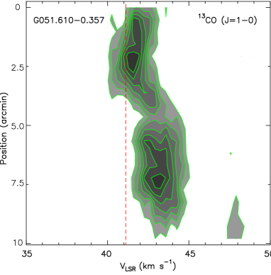
Fig. 10 : Position-Velocity diagrams of the ¹³CO $J$=1-0 emission along the filament associated with G051.610-0.357 (see the long dashed lines from top to bottom in Fig. 9). The black dashed line marks the RRL velocity of 41.1 km s^-1.

For the three bipolar bubbles (G049.998-0.125, G050.489+0.993, and G051.610-0.357), both the ionized gas and hot dust emission show a single structure. We suggest that each bipolar bubble is created by a single H II region. Both G049.998-0.125 and G051.610-0.357 are associated with a filament, respectively. The filament related to G049.998-0.125 contains two ATLASGAL clumps, which are dense and massive enough to potentially form massive stars. Figure 10 shows the position-velocity (PV) diagram constructed from the ¹³CO $J$=1-0 emission along the long filament coincident with G051.610-0.357. Since our observations did not resolve the bipolar structure of G049.998-0.125, we only made the PV diagram for the filament associated with G051.610-0.357. From the Fig. 10, we can discern that the filament is a single coherent object. In CO emission, both the filaments are perpendicular to G049.998-0.125 and G051.610-0.357, and divides them into two lobes. G051.610-0.357 has two symmetrical lobes. The central position of H II region is located on the filament for G051.610-0.357. For G049.998-0.125, the left lobe is smaller than the right lobe, it is because the central position of H II region associated with G049.998-0.125 is far from the filament, through comparing Fig. 1 and Fig. 7. The bipolar bubble forms when ionization front breaks through the two opposite faces of the sheet-like cloud simultaneously (Deharveng et al., 2010, 2015). From our observed results for G049.998-0.125 and G051.610-0.357, they are very similar to that of (Deharveng et al., 2010, 2015). We suggested that the exciting stars of G049.998-0.125 and G051.610-0.357 are formed in the sheet-like structure clouds. The sheet only observed edge-on appears as a filament. Moreover, the two lobes of G050.489+0.993 is associated with a clump, not a filament. Hence, we can not explain how bipolar bubble G050.489+0.993 forms. The clump shows a triangle-like shape with an integrated intensity gradient toward the direction of G050.489+0.993. Slice profiles of the ¹³CO $J$=1-0 emission are shown in Fig. 11 through the clump in two directions. The two cutting directions are shown as the green arrows in Fig. 8. We found a steep rise at the edges of the clump coincident with G050.489+0.993, as shown in black arrow in Fig. 11. This steep rise indicates that the two edges of the clump have been compressed by the expansion from the two lobes of bipolar bubble G050.489+0.993. We suggest that the shocks from this bipolar bubbles have expanded into the pre-existing clump, and have compressed it.

Fig. 11 : Slice profiles of ¹³CO $J$=1-0 emission through the clump in two directions. The cutting paths are shown as the green arrows in Fig. 8. The black arrow shows a distribution of steep rise.

5 CONCLUSIONS

We performed the molecular ¹²CO $J$=1-0, ¹³CO $J$=1-0 and C¹⁸O $J$=1-0, infrared, and radio continuum studies towards four bipolar bubbles. The four bipolar bubbles displays the bipolar structure at the 8.0 $\mu$m. From CO observations, we found that G045.386-0.726 is not a bipolar bubble, but the overlaping two bubbles with different distances along our sight of line. One of the two bubbles is related to a filament. The filament displays an arc-like structure with a steep integrated intensity gradient toward the bubble. We concluded that the filament is a sheet with a thickness of less than a few parsecs rather than a cylindrical filament. Both G049.998-0.125 and G051.610-0.357 are associated with a filament, while G050.489+0.993 is coincident with a clump. The molecular gas in coincidence with the three bipolar bubbles are the giant molecular cloud. The filaments in CO emission are perpendicular to G049.998-0.125 and G051.610-0.357, and divide them into two lobes. We suggested that the exciting stars of these two bipolar bubbles are formed in a sheet-like structure cloud. Moreover, the clump associated with G050.489+0.993 shows a triangle-like shape with an integrated intensity gradient toward the two lobes of G050.489+0.993, indicating that bipolar bubble G050.489+0.993 have expanded into the clump.

Acknowledgements We thank the referee for his/her report which helps to improve the quality of the paper. We are also grateful to the staff at the Qinghai Station of PMO for their assistance during the observations. This work was supported by the National Natural Science Foundation of China (Grant No. 11363004 and 11403042.)

References

- Anderson et al. (2011) Anderson, L. D., Bania, T. M., Balser, D. S., & Rood, R. T. 2011, Astrophys. J., 194, 32
- André et al. (2014) André, P., Di Francesco, J., Ward-Thompson, D., et al. 2014, Protostars and Planets VI, 27
- Bania et al. (2012) Bania, T. M., Anderson, L. D., & Balser, D. S. 2012, 759, 2
- Benjamin et al. (2003) Benjamin, R. A., Churchwell, E., & Babler, B. L., 2003, PASP, 115, 953
- Beaumont & Williams (2010) Beaumont, C. N., & Williams, J. P. 2010, Astrophys. J., 709, 791
- Castets et al. (1982) Castets, A., Langer, W. D., & Wilson, R. W. 1982, Astrophys. J., 262, 590
- Churchwell et al. (2006) Churchwell, E., Povich, M. S., Allen, D., et al. 2006, Astrophys. J., 649, 759
- Condon et al. (1998) Condon, J. J., Cotton, W. D., Greisen, E. W., et al. 1998, Astron. J., 115, 1693
- Csengeri et al. (2014) Csengeri, T., Urquhart, J. S., Schuller, F., et al. 2014, Astron. Astrophys., 565, A75
- Deharveng et al. (2003) Deharveng, L., Lefloch, B., Zavagno, A., et al. 2003, Astron. Astrophys., 408, 25
- Deharveng et al. (2010) Deharveng, L., Schuller, F., Anderson, L. D., et al. 2010, Astron. Astrophys., 523, A6
- Deharveng et al. (2015) Deharveng, L., Zavagno, A., Samal, M. R., et al. 2015, Astron. Astrophys., 582, A1
- Elmegreen (1998) Elmegreen, B. G. 1998, in ASP Conf. Ser., 148, 150, ed. C. E. Woodward, J. M. Shull, & H. A. Tronson
- Garden et al. (1991) Garden, R. P., Hayashi, M., Hasegawa, T., et al. 1991, Astrophys. J., 374, 540
- Inoue (2001) Inoue, A. K. 2001, AJ, 122, 1788
- Kauffmann & Pillai (2010) Kauffmann, J., & Pillai, T. 2010, Astrophys. J., 723, L7
- Lèger & Puget (1984) Lèger, A., & Puget, J. L. 1984, Astron. Astrophys., 137, 5
- Martins et al. (2005) Martins, P. G., Schaerer, D., & Hillier, D. J. 2005, Astron. Astrophys., 436, 1049
- Mezger et al. (1974) Mezger, P. G., Smith, L. F., & Churchwell, E. 1974, Astron. Astrophys., 32, 26
- Ossenkopf & Henning (1994) Ossenkopf, V., & Henning, T. 1994, Astron. Astrophys., 291, 943
- Pomarè s et al. (2009) Pomarès, M., Zavagno, A., Deharveng, L., et al. 2009, Astron. Astrophys., 496, 177
- Reid et al. (2016) Reid, M. J., Dame, T. M., Menten, K. M., & Brunthaler, A. 2016, Astrophys. J., 823, 77
- Rieke & Lebofsky (1985) Rieke, G. H., & Lebofsky, M. J. 1985, Astrophys. J., 288, 618
- Rieke et al. (2004) Rieke, G. H., Young, E. T., Engelbracht, C. W., et al. 2004, Astrophys. J. Suppl. Ser., 154, 25
- Schuller et al. (2009) Schuller, F., Menten, K. M., Contreras, Y. et al. 2009, Astron. Astrophys., 504, 415
- Skrutskie et al. (2006) Skrutskie, M. F., Cutri, R. M., Stiening, R., et al. 2006, Astron. J., 131, 1163
- Watson et al. (2008) Watson, C., Povich, M. S., Churchwell, E. B., et al. 2008, Astrophys. J., 681, 1341
- Xu et al. (2013) Xu, J.-L., Wang, J.-J., Liu, X.-L., et al. 2013, Astron. Astrophys., 559, 113
- Xu & Ju (2014a) Xu, J.-L., & Ju, B.-G. 2014a, Astron. Astrophys., 569, 36
- Xu et al. (2014b) Xu, J.-L., Wang, J.-J., Ning, C.-C., et al. 2014b, RAA, 14, 47
- Zhang et al. (2016) Zhang, C.-P., Li, G.-X., Wyrowski, F., et al. 2016, 585, A117
- Treu et al. (2003) Treu, T. et al., 2003, Astrophys. J., 591, 53