A survey of closed self-shrinkers with symmetry

Abstract.

In this paper, we survey known results on closed self-shrinkers for mean curvature flow and discuss techniques used in recent constructions of closed self-shrinkers with classical rotational symmetry. We also propose new existence and uniqueness problems for closed self-shrinkers with bi-rotational symmetry and provide numerical evidence for the existence of new examples.

1. Introduction

The self-shrinking solitons for mean curvature flow are ancient solutions to the flow that evolve by “shrinking” self-similarly about a point. A time-slice for a self-shrinking flow is a hypersurface, called a self-shrinker, that satisfies a non-linear second order elliptic equation involving the mean curvature. When the flow shrinks about the origin, the self-shrinker equation for a time-slice $\Sigma$ is

$${\Delta}_{{\mathbf{g}}_{{}_{\Sigma}}}\mathbf{X}=\alpha{\mathbf{X}}^{\bot},$$

where $\alpha<0$ is a constant and ${\Delta}_{{\mathbf{g}}_{{}_{\Sigma}}}\mathbf{X}$ equals to the mean curvature vector for $\Sigma$.

The first variation formula shows that self-shrinkers are minimal hypersurfaces in the Riemmanian manifold $\mathbb{R}^{n+1}$ with conformal metric

$$e^{\frac{\alpha|\mathbf{X}|^{2}}{n}}\left({dx_{1}}^{2}+\cdots+{dx_{n+1}}^{2}\right).$$

This geometric variational characterization leads to the reduction that self-shrinkers with rotational or bi-rotational symmetry correspond to geodesics in the plane equipped with induced conformal metrics. So, the existence and uniqueness of closed self-shrinkers with one of these types of symmetry can be reduced to the study of closed geodesics in two dimensional manifolds.

Self-shrinkers play a vital role in the theory of mean curvature flow and admit a number of interesting applications. Husiken’s monotonicity formula [38, Section 3] shows that self-shrinkers model the asymptotic behavior of mean curvature flow at type I singularities. Self-shrinkers can also be used as barriers to explore different phenomena for solutions to mean curvature flow. For instance, the existence of a self-shrinking torus was recently used in [18] to construct initial entire graphs whose mean curvature flow evolves away from the heat flow.

The focus of this survey is on closed self-shrinkers with rotational or bi-rotational symmetry. The paper is organized as follows:

• In Section 2, we introduce the self-shrinker equation and highlight various elliptic and parabolic characterizations of self-shrinkers.

• In Section 3, we discuss existence and uniqueness results for closed self-shrinkers. We begin with the classification of self-shrinking curves in ${\mathbb{R}}^{2}$, including proofs of two geometric conservation laws for self-shrinking curves [1, 22, 28]. Next, we review rigidity results for closed self-shrinkers due to Huisken [37, 38] and Brendle [12]. Finally, we mention several examples of self-shrinkers with symmetry [9, 16, 20, 49].

• In Section 4, we give a detailed sketch of the recent variational proof for the existence of an embedded, torus self-shrinker with rotational symmetry [19]. The proof uses a modified curve shortening flow to find a closed geodesic in the upper half-plane. A new feature of this variational proof is that it comes with an upper bound for the weighted length of the constructed geodesic.

• In Section 5, we expand on how the shooting method can be used to construct closed self-shrinkers with rotational symmetry. In the first part of this section, we outline the analysis used in [16] to construct an immersed sphere self-shrinker with rotational symmetry. Then, we illustrate how the behavior of geodesics for three shooting problems can be used to generate more examples of closed self-shrinkers with rotational symmetry [20]. We end this section with a discussion on the role of continuity in the shooting method.

• In Section 6, we consider the problem of constructing closed self-shrinkers with bi-rotational symmetry. Here we propose the existence of various bi-rotational ${\mathbb{T}}^{3}$ and ${\mathbb{S}}^{3}$ self-shrinkers in ${\mathbb{R}}^{4}$ and present numerical approximations of their symmetric profile curves.

• Finally, in Section 7, we present a list of old and new open problems on the existence and uniqueness of closed self-shrinkers.

2. Elliptic and parabolic characterizations of self-shrinkers

2.1. Self-shrinker equation

A hypersurface $\Sigma$ in Euclidean space ${\mathbb{R}}^{n+1}$ is a self-shrinker with the constant coefficient $\alpha<0$ when it solves the quasi-linear elliptic partial differential system of second order

(2.1) $${\Delta}_{{\mathbf{g}}_{{}_{\Sigma}}}\mathbf{X}=\alpha{\mathbf{X}}^{\bot},$$

where $\mathbf{X}$ is the position vector for $\Sigma$, ${\mathbf{g}}_{{}_{\Sigma}}$ is the induced metric on $\Sigma$, ${\Delta}_{{\mathbf{g}}_{{}_{\Sigma}}}$ is the Laplace-Beltrami operator for ${\mathbf{g}}_{{}_{\Sigma}}$, and $\mathbf{X}^{\bot}$ is the orthogonal projection of $\mathbf{X}$ into the normal bundle of $\Sigma$. We note that ${\Delta}_{{\mathbf{g}}_{{}_{\Sigma}}}\mathbf{X}$ equals the mean curvature vector $\mathbf{H}$ for $\Sigma$. When we orient $\Sigma$ by a smooth unit normal vector field $\mathbf{N}$ and introduce the mean curvature $H=\mathbf{H}\cdot\mathbf{N}=\left({\Delta}_{{\mathbf{g}}_{{}_{\Sigma}}}\mathbf{X}\right)\cdot\mathbf{N}$, we obtain the the scalar partial differential equation

(2.2) $$H=\alpha\,{\mathbf{X}}\cdot\mathbf{N}.$$

Though (2.2) resembles the classical constant mean curvature equation, in general, the standard techniques (such as method of moving planes) do not directly work for self-shrinkers.

Locally, a self-shrinker may be written as the graph of a function $u:\Omega\subset\mathbb{R}^{n}\to\mathbb{R}$, where $u$ is a solution to

(2.3) $$\textrm{div}_{\mathbb{R}^{n}}\left(\frac{Du}{\sqrt{1+|Du|^{2}}}\right)=\alpha\frac{u-x\cdot Du}{\sqrt{1+|Du|^{2}}}.$$

2.2. Ancient solutions for mean curvature flow

A self-shrinker $\Sigma$ corresponds to the $t=\left(t_{0}+\frac{1}{2\alpha}\right)$ time slice of a mean curvature flow that shrinks to the origin at the extinction time $t_{0}$. More explicitly, the one parameter family of hypersurfaces

$${\Sigma}_{t}:=\sqrt{2\alpha\left(t-t_{0}\right)\,}\,{\Sigma}$$

is a solution to mean curvature flow (MCF)

(2.4) $$\left(\frac{\partial}{\partial t}\mathbf{X}(\cdot,t)\right)^{\bot}=\mathbf{H}(\cdot,t),$$

for all ancient time $t\in\left(-\infty,t_{0}\right)$. Here $\mathbf{H}(\cdot,t)$ denotes the mean curvature vector for the time slice ${\Sigma}_{t}$. It follows that self-shrinkers correspond to ancient solutions to MCF that evolve over time by homotheties.

2.3. Monotonicity of the Gaussian area

Consider the backward heat kernel $\rho\left(\mathbf{X},\,t\right)=\frac{1}{{\left(4\pi\left(t_{0}-t\right)\,\right)}^{\frac{n}{2}}}e^{-\,\frac{{|\mathbf{X}|}^{2}}{4\left(t_{0}-t\right)}}$ for the backward heat equation $f_{t}=-{\Delta}_{{\mathbb{R}}^{n+1}}f$. Huisken [38, Section 3] showed that closed hypersurfaces evolving under MCF, for $t<t_{0}$, satisfy

(2.5) $$\frac{\partial}{\partial t}\int_{\Sigma_{t}}\rho=-\int_{\Sigma_{t}}\rho\,{\left|\,\mathbf{H}+\frac{1}{2\left(t_{0}-t\,\right)}{\mathbf{X}}^{\bot}\right|}^{2}\leq 0.$$

It follows from this monotonicity formula that mean curvature flow behaves asymptotically like a self-shrinker at a singularity where the curvature does not blow-up too fast [38, Theorem 3.5]. Also, see Hamilton’s monotonicity formula [30] and the local monotonicity formula due to Ecker [21].

2.4. Minimality of self-shrinkers

The first variation formula for weighted area (Ilmanen’s lecture notes [40, Section 2] and Morgan’s book [48, Chapter 18]) shows that self-shrinkers are variational objects. A submanifold $\Sigma$ immersed in a Riemannian manifold $\left(\mathcal{M},g\right)$ with density $e^{\Psi}$ is minimal if and only if its weighted mean curvature vector ${\mathbf{H}}_{\Psi}={\mathbf{H}}-{\left({\nabla}_{\mathcal{M}}\Psi\right)}^{\bot}$ vanishes, where $\mathbf{H}$ denotes the mean curvature vector field on $\Sigma$ in $\left(\mathcal{M},g\right)$ and ${\left({\nabla}_{\mathcal{M}}\Psi\right)}^{\bot}$ is the orthogonal projection of the vector field ${\nabla}_{\mathcal{M}}\Psi$ into the normal bundle of $\Sigma$. Given a hypersurface $\Sigma$ in ${\mathbb{R}}^{n+1}$ and constant $\alpha<0$, the following three statements are equivalent to each other:

• $\Sigma$ is critical for the Gaussian area functional ${\int}_{\Sigma}\;e^{\frac{\alpha|\mathbf{X}|^{2}}{2}}{dvol}_{\Sigma}$.

• $\Sigma$ satisfies the Euler-Lagrange equation ${\Delta}_{{\mathbf{g}}_{{}_{\Sigma}}}\mathbf{X}={\left[\,{\nabla}_{{\mathbb{R}}^{n+1}}\left(\frac{\alpha\,{|\mathbf{X}|}^{2}}{2}\;\right)\,\right]}^{\bot}=\alpha\mathbf{X}^{\bot}$ for the Gaussian area.

• $\Sigma$ is a minimal submanifold in the Riemmanian manifold ${\mathbb{R}}^{n+1}$ with metric $e^{\frac{\alpha|\mathbf{X}|^{2}}{n}}\left({dx_{1}}^{2}+\cdots+{dx_{n+1}}^{2}\right)$.

2.5. Minimal cones as self-shrinkers

The Clifford cone ${x_{1}}^{2}+{x_{2}}^{2}={x_{3}}^{2}+{x_{4}}^{2}$ over the Clifford torus in ${\mathbb{S}}^{3}$ is a self-shrinker in ${\mathbb{R}}^{4}$. More generally, whenever ${\mathcal{S}}^{n-1}$ is a minimal hypersurface in the round hypersphere ${\mathbb{S}}^{n}$, its cone $C\left(\mathcal{S}\right):=\left\{r\mathbf{p}\,:\,r\in\mathbb{R},\mathbf{p}\in\mathcal{S}\right\}$ becomes a minimal hypersurface in ${\mathbb{R}}^{n+1}$. Since ${\mathbf{X}}\cdot\mathbf{N}=0$ on $C\left(\mathcal{S}\right)$, it follows that a minimal cone is a self-shrinker satisfying $H=0=\alpha\,{\mathbf{X}}\cdot\mathbf{N}$ for any coefficient $\alpha$.

2.6. Normalization of the coefficient

Without loss of generality, we can use dilations to normalize the coefficient $\alpha<0$. In the literature, two normalizations $\alpha=-1$ (for instance, [38]) and $\alpha=-\frac{1}{2}$ (for instance, [14]) are common. Unless otherwise noted, we take the normalization $\alpha=-\frac{1}{2}$ for the remainder of the survey.

3. Results on existence and uniqueness of closed self-shrinkers

3.1. Shrinking curves in the plane

In 1956, Mullins [52] introduced the one-dimensional mean curvature flow, the curve shortening flow, in $\mathbb{R}^{2}$ and constructed examples of solitons for the flow. In 1986, Gage and Hamilton [25] solved the shrinking conjecture by showing that a convex curve collapses to a round point under the curve shortening flow. The curve remains convex and becomes circular as it shrinks, in the sense that the ratio of the inscribed radius to the circumscribed radius approaches $1$, the ratio of the maximum curvature to the minimum curvature approaches $1$, and the higher order derivatives of the curvature converge to $0$ uniformly.

In 1987, Grayson [27] proved the striking result that an embedded, not necessarily convex, closed curve eventually becomes convex, and therefore it eventually contracts to a round point, under the curve shortening flow. In 1998, Huisken gave a concise proof [39] of Grayson’s Theorem, using a distance comparison argument and the classification and characterization of solitons as asymptotic models for singularities. We refer the interested reader to recent proofs by Andrews-Bryan [5, 6] and Magni-Mantegazza [46].

In the mid 1980’s, Abresch-Langer [1] and Epstein-Weinstein [22] independently investigated the self-shrinking solitons for the curve shortening flow. Here are numerical approximations of some of self-shrinkers:

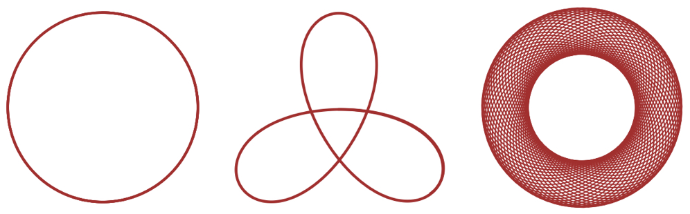
Figure 1. Examples of self-shrinkers for the curve shortening flow.

Unlike higher dimensional cases, the one-dimensional self-shrinker equation admits explicit first integrals.

Theorem 1 (Geometric conservation laws for self-shrinking curves, [1, 22, 28]).

Let the function $\kappa$ denote the curvature of an immersed non-flat self-shrinker with the coefficient $\alpha<0$ in the $xy$-plane.

1. The quantity $\kappa\,e^{\alpha\left(\frac{{x}^{2}+{y}^{2}}{2}\right)}$ is constant. Hence, the curvature $\kappa$ is an increasing function of the radius $\sqrt{x^{2}+y^{2}}$.

2. The entropy ${\kappa}^{2}+\alpha\ln\left({\kappa}^{2}\right)+{\left(\frac{d\kappa}{d\theta}\right)}^{2}$ is constant, where $\theta$ is the angle between the tangent vector and the $x$-axis.

Proof.

Let ${\mathbf{X}}(s)=\left(x(s),y(s)\right)$ denote an immersed non-flat self-shrinker parameterized by an arc length $s$. We introduce the angle function $\theta(s)$ between the unit tangent vector $T(s)=\frac{d{\mathbf{X}}}{ds}$ and the $x$-axis, the unit normal vector $\mathbf{N}(s)=\mathrm{J}\,\mathbf{T}(s)$ (with the $\frac{\pi}{2}$-rotation $\mathrm{J}$), the signed curvature $\kappa(s)=\frac{d\theta}{ds}$, tangential support function $\tau(s)={\mathbf{X}}(s)\cdot\mathbf{T}(s)$, and normal support function $\nu(s)={\mathbf{X}}(s)\cdot\mathbf{N}(s)$. Combining the self-shrinker equation $\kappa(s)=\alpha\,\nu(s)$ with the coefficient $\alpha<0$ and the structure equations for the curve

(3.1) $$\frac{d\tau}{ds}=1+\kappa\nu,\quad\frac{d\nu}{ds}=-\kappa\tau,\quad\frac{d}{ds}\left(\frac{{\tau}^{2}+{\nu}^{2}}{2}\right)=\tau,\quad x^{2}+y^{2}={\tau}^{2}+{\nu}^{2}$$

implies the conservation law

$$\frac{d}{ds}\left[\kappa\,e^{\alpha\left(\frac{{x}^{2}+{y}^{2}}{2}\right)}\right]=\frac{1}{\alpha}\,\frac{d}{ds}\left(\nu\,e^{\alpha\left(\frac{{\tau}^{2}+{\nu}^{2}}{2}\right)}\right)=\frac{1}{\alpha}\left(-\kappa+\alpha\nu\right)\,\tau\,e^{\alpha\left(\frac{{\tau}^{2}+{\nu}^{2}}{2}\right)}=0,$$

which guarantees that the geometric quantity $\kappa\,e^{\alpha\left(\frac{{x}^{2}+{y}^{2}}{2}\right)}$ is constant on the self-shrinker ([28, Lemma 5.5] for $\alpha=-1$ and [1, Theorem A]). Reading the first two structure equations (3.2) with respect to the angle $\theta$ yields

(3.2) $$\frac{d\tau}{d\theta}=\frac{1}{\kappa}+\nu,\quad\frac{d\nu}{d\theta}=-\tau,\quad\frac{1}{\kappa}=-{\nu}_{\theta\theta}-\nu.$$

Combining these and the self-shrinker equation $\kappa=\alpha\,\nu$ implies the conservation law ([22, Section 1] for $\alpha=-1$):

$$\frac{d}{d\theta}\left[{{\kappa}_{\theta}}^{2}+{\kappa}^{2}+\alpha\ln\left({\kappa}^{2}\right)\right]=2{\kappa}_{\theta}\left[{\kappa}_{\theta\theta}+\kappa+\frac{\alpha}{\kappa}\right]=2{\kappa}_{\theta}\,\alpha\left[\left({\nu}_{\theta\theta}+\nu\right)+\frac{1}{\kappa}\right]=0.$$

∎

Recently, classification results and conservation laws for self-shrinkers were developed in other geometric contexts by Halldorsson [28, 29] and Chang [13].

3.2. Rigidity results for self-shrinkers

Round spheres admit geometric characterizations both as constant mean curvature (CMC) surfaces and as self-shrinkers for the mean curvature flow. The classical theorems of Jellett, Alexandrov, and Hopf show that round spheres posses some rigidity as CMC hypersurfaces. Jellett’s Theorem in ${\mathbb{R}}^{3}$ and its generalization [26, 35, 36, 44, 50], which uses Hsiung-Minkowski integral formulas [35, 36], confirms that a closed, star-shaped, CMC hypersurface is round. Alexandrov used his method of moving planes to prove that an embedded, closed CMC hypersurface in ${\mathbb{R}}^{n+1}$ must be a round sphere. The embedded assumption is essential due to the existence of immersed tori in ${\mathbb{R}}^{3}$ with positive constant mean curvature, see Abresch [2] and Wente [53]. Hopf showed if a closed immersed CMC surface in ${\mathbb{R}}^{3}$ is a topological sphere, then it must be round. One of Hopf’s two proofs [31] exploits a beautiful fact that the Codazzi equation implies the existence of globally well-defined holomorphic quadratic differential on CMC surfaces. The proof can be generalized to a wider class of surfaces in more general ambient spaces, for instance, as in [3, 11, 23].

Despite the similarity between the CMC and self-shrinker equations, the classical rigidity results of Alexandrov and Hopf for CMC hypersurfaces do not hold for self-shrinkers. (There are examples of an embedded $\mathbb{S}^{1}\times\mathbb{S}^{n-1}$ self-shrinker and an immersed, non-round $\mathbb{S}^{n}$ self-shrinker in $\mathbb{R}^{n+1\geq 3}$.) In addition, analogues of the classical Weierstrass-Enneper representation (holomorphic resolution of minimal surfaces) or Kenmotsu representation (which prescribes harmonic Gauss map of CMC surfaces [42]) are not known for self-shrinkers. However, just as in the CMC setting, round spheres do posses some rigidty as closed self-shrinkers.

In 1984, Huisken [37] established that a convex hypersurface in ${\mathbb{R}}^{n+1\geq 3}$ shrinks to a round point by showing that the hypersurface, under a rescaled flow, converges to a totally umbilical hypersurface. Hence, Huisken’s result in ${\mathbb{R}}^{n+1\geq 3}$ is a higher dimensional analogue of the Gage-Hamilton Theorem for the curve shortening flow in ${\mathbb{R}}^{2}$. Since self-shrinkers keep their shape under the flow, these parabolic asymptotic convergence results implicitly imply the elliptic rigidity result that a closed, convex self-shrinker in any dimension is round. We highlight two additional rigidity results for closed self-shrinkers:

• Rigidity of spheres as mean-convex self-shrinkers in ${\mathbb{R}}^{n+1\geq 3}$: In 1990, Huisken [38, Theorem 4.1] showed that a closed, mean-convex ($H>0$) self-shrinker must be a round sphere. The key starting point in his argument is to combine the self-shrinker equation and Simons’ identity for the squared length ${|A|}^{2}$ of the second fundamental form to obtain an explicit expression for the Laplacian of the well-defined quotient function $\frac{{|A|}^{2}}{H^{2}}$. Since the self-shrinker is compact, the maximum principle guarantees that $\frac{{|A|}^{2}}{H^{2}}$ is constant. Subsequent analysis of the pde for $\frac{{|A|}^{2}}{H^{2}}$ and Hsiung-Minkowski integral formulas ultimately lead to the conclusion that the mean curvature $H$ is a positive constant. Now, a mean-convex self-shrinker has positive support function. Therefore, the self-shrinker is round. See also Montiel’s Theorem [50].

• Rigidity of spheres as embedded ${\mathbb{S}}^{2}$ self-shrinkers in ${\mathbb{R}}^{3}$: In 2016, Brendle [12] proved the long-standing Alexandrov-Hopf type conjecture showing that an embedded, topological $\mathbb{S}^{2}$ self-shrinker in ${\mathbb{R}}^{3}$ must be a round sphere. Unlike in the CMC case, combining the self-shrinker equation with the Codazzi equations does not produce a holomorphic quadratic differential on self-shrinkers, so the Hopf type approach does not directly work for self-shrinkers. The key result in Brendle’s proof is that the sign of the normal support function does not change on an embedded ${\mathbb{S}}^{2}$ self-shrinker in ${\mathbb{R}}^{3}$, i.e., the closed, embedded self-shrinker is star-shaped. Thus, the self-shrinker is mean-convex (by the definition of the self-shrinker equation), and by Huisken’s Rigidity Theorem it is a round sphere.

3.3. Examples of self-shrinkers

Though round spheres are rigid as CMC hypersurfaces and self-shrinkers under certain additional assumptions, there are numerous examples that contrast the rigidity results from the previous section. Hsiang-Teng-Yu [33] proved that there exist infinitely many distinct CMC immersions of ${\mathbb{S}}^{2k-1}$ in ${\mathbb{R}}^{2k\geq 4}$, see also [34]. These examples come from studying closed hypersurfaces with bi-rotational symmetry. (We consider the problem of constructing closed self-shrinkers with bi-rotational symmetry in Section 6.) A rich source of examples of immersed self-shrinkers comes from hypersurfaces with rotational symmetry. Using the shooting method for geodesics (see Section 5), an infinite number of complete, self-shrinkers for each of the rotational topological types: $\mathbb{S}^{n}$, $\mathbb{S}^{1}\times\mathbb{S}^{n-1}$, $\mathbb{R}^{n}$, and $\mathbb{S}^{1}\times\mathbb{S}^{n-1}$ were constructed in [20].

In the following, we introduce the geodesic equation for the profile curve of a self-shrinker with rotational symmetry and highlight a few modern examples of closed self-shrinkers. We note that even though rotational self-shrinkers have a variational characterization, it is unknown if the geodesic equation is integrable.

• Profile curves of rotational shrinkers as geodesics in the half-plane: Self-shrinkers are minimal submanifolds in the Remannian manifold $\mathbb{R}^{n+1\geq 3}$ equipped with the conformal metric $e^{-\frac{|\mathbf{X}|^{2}}{2n}}\left({dx_{1}}^{2}+\cdots+{dx_{n+1}}^{2}\right).$ Applying the first variation formula to a rotational hypersurface $\mathbf{X}(s,\omega)=\left(x(s),r(s)\omega\right)$, $s\in\mathbb{R}$, $\omega\in\mathbb{S}^{n-1}$, with the profile curve $(x(s),r(s))$ in the half-plane $\mathbb{H}=\{(x,r)\in\mathbb{R}^{2}\,|\,r>0\}$, shows that it is a self-shrinker if and only if its profile curve is a geodesic for the conformal metric

  $$g_{Ang}=r^{2(n-1)}e^{-\frac{x^{2}+r^{2}}{2}}(dx^{2}+dr^{2}).$$

  The geodesic equation for the profile curve $(x(s),r(s))$ of a self-shrinker with rotational symmetry is

  $$\frac{x^{\prime}r^{\prime\prime}-x^{\prime\prime}r^{\prime}}{x^{\prime 2}+r^{\prime 2}}=\left(\frac{n-1}{r}-\frac{r}{2}\right)x^{\prime}+\frac{1}{2}xr^{\prime},$$

  and the Gauss curvature of the Riemannian manifold $(\mathbb{H},g_{Ang})$ is given by

  $$K=\frac{r^{2}+(n-1)}{r^{2n}}e^{\frac{x^{2}+r^{2}}{2}}>0.$$

• The fundamental examples of rotational self-shrinkers: The sphere of radius $\sqrt{2n}$ centered at the origin, a flat plane through origin, and a round cylinder of radius $\sqrt{2(n-1)}$ with axis through the origin are examples of self-shrinkers with rotational symmetry. We have the following profile curves for these fundamental examples:

  • Round sphere: $x^{2}+r^{2}=2n$ with the profile curve $(x(s),r(s))=\left(\sqrt{2n}\cos\left(\frac{s}{\sqrt{2n}}\right),\sqrt{2n}\sin\left(\frac{s}{\sqrt{2n}}\right)\right)$.

  • Flat plane: $x\equiv 0$ with the profile curve $(x(s),r(s))=(0,s)$.

  • Round cylinder: $r\equiv\sqrt{2(n-1)}$ with the profile curve $(x(s),r(s))=(s,\sqrt{2(n-1)})$.

• Angenent’s torus: Using the shooting method for geodesics, Angenent [9] gave the first proof of the existence of an embedded torus ($\mathbb{S}^{1}\times\mathbb{S}^{n-1}$) self-shrinker in $\mathbb{R}^{n+1}$ with a rotational symmetry. See also [16, 19, 49].

  

  Figure 2. The profile curve whose rotation about the horizontal axis is an embedded torus self-shrinker.

• Immersed sphere self-shrinker: Motivated by Angenent’s construction and using the shooting method from the axis of rotation, it was shown in [16] that there exists an immersed and non-embedded $\mathbb{S}^{n}$ self-shrinker in $\mathbb{R}^{n+1}$ with a rotational symmetry (see Section 5.1 for a detailed sketch of the proof). The existence of this immersed self-shrinkers explains why the embeddedness assumption is essential in Brendle’s rigidity result for embedded $\mathbb{S}^{2}$ self-shrinkers in $\mathbb{R}^{3}$ [12].

  

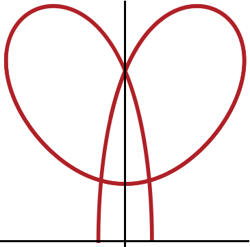
  Figure 3. The profile curve whose rotation about the horizontal axis is an immersed sphere self-shrinker.

• Immersed self-shrinkers: Building on the work in [9, 16, 43], infinitely many immersed and non-embedded self-shrinkers for each of the rotational topological types: $\mathbb{S}^{n}$, $\mathbb{S}^{1}\times\mathbb{S}^{n-1}$, $\mathbb{R}^{n}$, and $\mathbb{S}^{1}\times\mathbb{R}^{n-1}$ were constructed in [20]. The main idea for the construction is to study the behavior of solutions to the geodesic equation near two known self-shrinkers and use continuity arguments to find complete self-shrinkers between them. See Section 5.2 for illustrations on how to carry out this heuristic.

  

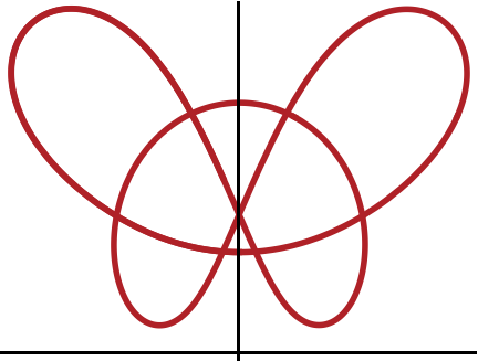
  Figure 4. The profile curve whose rotation about the horizontal axis is an immersed torus self-shrinker.

• Møller’s embedded shrinkers with higher genus in $\mathbb{R}^{3}$: In 2011, Møller [49] performed a smooth desingularization of two rotational self-shrinkers: Angenent’s torus and the round sphere. Møller’s shrinkers are generalizations of Costa’s embedded three-end minimal surface [32], which can be viewed as a smooth desingularization of two rotational minimal surfaces: a catenoid and a plane passing the neck of the catenoid. More concretely, Møller proved the existence of a large lower bound $N_{0}$ such that for each even $g=2k\geq N_{0}$ there exists a closed self-shrinker ${\Sigma}_{g}$ in $\mathbb{R}^{3}$ with genus $g$ that is invariant under the dihedral symmetry group with $2g$ elements. Furthermore, the sequence of self-shrinkers ${\Sigma}_{g}$ converges in the Hausdorff sense (and smoothly away from the two initial intersection circles) to the union of Angenent’s torus and the round sphere.

  

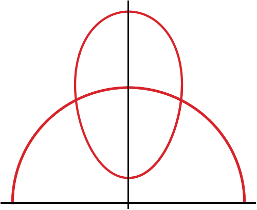
  Figure 5. Two intersecting geodesics in Møller’s desingularization of self-shrinking tori and round sphere

4. Variational method for an embedded $\mathbb{S}^{1}\times\mathbb{S}^{n-1}$ self-shrinker in $\mathbb{R}^{n+1}$

In this section, we outline the parabolic proof from [19] of the existence of a rotational self-shrinking torus. The proof uses variational techniques, applied to the geodesic problem from Section 3.3, to find a simple, closed geodesic and gives an estimate for the length of this geodesic in $(\mathbb{H},g_{Ang})$. It is unknown if this proof recovers the closed geodesics constructed in [9]. (See Section 7.)

Theorem 2 ([19]).

For $n\geq 2$, there exists a simple, closed geodesic $\gamma_{\infty}$, for the conformal metric

$$g_{Ang}=r^{2(n-1)}e^{-(x^{2}+r^{2})/2}(dx^{2}+dr^{2})$$

on the half-plane $\mathbb{H}=\{(x,r)\in\mathbb{R}^{2}\,|\,r>0\}$. Moreover, its length $L_{n}(\gamma_{\infty})$ in the metric $g_{Ang}$ is less than the length of the double cover of the half-line $x=0$:

$$L_{n}(\gamma_{\infty}):=\int_{\mathbb{S}^{1}}r^{n-1}e^{-(x^{2}+r^{2})/4}\sqrt{x^{\prime 2}+r^{\prime 2}}du<2\int_{0}^{\infty}s^{n-1}e^{-s^{2}/4}ds.$$

The idea for finding this closed geodesic is to study a modified curve shortening flow:

(4.1) $$\frac{\partial}{\partial t}\gamma_{t}=\frac{k_{g}}{K}\bf{n},$$

where $k_{g}$ is the geodesic curvature and $K>0$ is the Gauss curvature in $(\mathbb{H},g_{Ang})$. The goal is to create an initial curve $\gamma_{0}$ whose evolution under the flow converges to the geodesic $\gamma_{\infty}$. To do this we consider a special family of initial curves and study their evolutions under the modified curve shortening flow. The advantage of this approach is that the evolution is well-known and the crux of the proof is in selecting the appropriate family of initial curves, all of which have length less than twice the length of the half-line $x=0$ and enclose Gauss area of exactly $2\pi$.

The modified curve shortening flow has two important properties.

• The flow decreases length: Since the arc length $ds$ evolves according to $\frac{\partial}{\partial t}ds=-\frac{k_{g}^{2}}{K}\,ds$, the length $L_{n}(\gamma_{t})$ is non-increasing:

  $$\frac{d}{dt}L_{n}(\gamma_{t})=-\int_{\gamma_{t}}\frac{k_{g}^{2}}{K}\,ds\leq 0.$$

• The flow preserves total Gauss area of $2\pi$: When the evolving curves $\gamma_{t}$ are simple, closed curves bounding domains $\Omega_{t}$, the Gauss-Bonnet formula gives

  $$\frac{d}{dt}\iint_{\Omega_{t}}KdA=-\oint_{\gamma_{t}}k_{g}\,ds=-2\pi+\iint_{\Omega_{t}}KdA.$$

  In particular, if the total Gauss area enclosed by the initial curve equals $2\pi$, then the total Gauss area enclosed by $\gamma_{t}$ is also $2\pi$ as long as the flow exists.

Working in regions where the Gaussian curvature is uniformly bounded from above and below away from 0, the short-time existence for the flow follows from [24, 7]. This gives the following long-time existence result.

Proposition 1 (Long-time existence).

Let $\gamma_{0}$ be a simple closed curve. If the domain $\Omega_{0}$ enclosed by $\gamma_{0}$ satisfies $\iint_{\Omega_{0}}KdA=2\pi$, then the evolution of $\gamma_{0}$ with normal velocity $k_{g}/K$ exists for all time.

By selecting a family of initial curves, all of which have length less than twice the length of the half-line $x=0$ and enclose total Gauss area of exactly $2\pi$, Proposition 1 guarantees that the evolutions of these curves exist for all time, and because the length decreases, the flow starting from each curve does not converge to a double cover of the half-line $\{x=0\}$. To select the family of initial curves, we consider rectangles $R[a,b,c]$ with vertices $(a,-c),(a,c),(b,c),(b,-c)$, $a<b$ and $c>0$.

Figure 6. The rectangle $R[a,b,c]$.

Numerics show that all the rectangles with $c=1/2$ will satisfy the requirement on length. To simplify computations, we take $c=c_{0}\approx 0.481$ to be the positive real number such that $\frac{e^{-c_{0}^{2}/4}}{\int_{0}^{c_{0}}e^{-x^{2}/4}dx}=2$.

Proposition 2.

For every $a,b\in(0,\infty)$ and $n\geq 2$, we have

(4.2) $$L_{n}(a,b,c_{0})<2\int_{0}^{\infty}s^{n-1}e^{-s^{2}/4}ds.$$

The proof of this result is by induction on the dimension and numerical verification on lower dimensions. The induction is quite involved and makes heavy use of Taylor expansions.

Proposition 3.

There is a smooth function $\varphi:\mathbb{R}_{+}\to\mathbb{R}_{+}$ with $\varphi(a)>a$, with $\lim_{a\to 0}\varphi(a)=0$, so that the family of rectangles $R[a,\varphi(a),c_{0}]$ satisfies

$$\iint_{R[a,\varphi(a),c_{0}]}KdA=2\pi,\quad L_{n}(a,\varphi(a),c_{0})<2\int_{0}^{\infty}s^{n-1}e^{-s^{2}/4}ds.$$

Next we consider the modified curve shortening flow for the initial curves $R[a,\varphi(a),c_{0}]$.

Proposition 4.

Let $\Phi:\mathbb{R}_{+}\times\mathbb{R}_{+}\to C^{0}(\mathbb{S}^{1},\mathbb{H})$ be the map with the following properties:

1. $\Phi(a,0)=R[a,\varphi(a),c_{0}]$,

2. For fixed $a$, $\Phi(a,t)$ satisfies the evolution equation (4.1).

There exists an $a_{0}\in\mathbb{R}_{+}$ so that $\Phi(a_{0},t)$ intersects the line $r=\sqrt{2(n-1)}$ for all time $t\in\mathbb{R}_{+}$.

Proof.

The set of curves that do not intersect the line $r=\sqrt{2(n-1)}$ is split into two disjoint sets

$$A_{1} =\{\text{continuous closed curves }\gamma:\mathbb{S}^{1}\to\mathbb{H}\mid\gamma(s)<r_{n},s\in S^{1}\},$$

$$A_{2} =\{\text{continuous closed curves }\gamma:\mathbb{S}^{1}\to\mathbb{H}\mid\gamma(s)>r_{n},s\in S^{1}\}.$$

The line $r=\sqrt{2(n-1)}$ is a geodesic (it is the profile curve for the round cylinder self-shrinker), so it is stationary under the modified curve shortening flow. By the maximum principle, if $\Phi(a,t_{0})\in A_{i}$ for some $i=1,2$ and some time $t_{0}$, then $\Phi(a,t)\in A_{i}$ for $t\geq t_{0}$. Consider the following subsets of $\mathbb{R}_{+}$:

$$U_{i} =\{a\in\mathbb{R}_{+}\mid\exists t>0,\Phi(a,t)\in A_{i}\}$$

Both $U_{1}$ and $U_{2}$ are open and $U_{1}\cap U_{2}=\emptyset$. Therefore $U_{1}\cup U_{2}\neq\mathbb{R}_{+}$, which proves the existence of $a_{0}$. ∎

The remainder of the proof of Theorem 2 is dedicated to showing that the curves $\gamma_{t}:=\Phi(a_{0},t)$ converge to a simple, closed geodesic that is symmetric about the $r$-axis and convex in the Euclidean sense. First, we show that on compact sets, the curves $\gamma_{t}$ approach a geodesic along a subsequence.

Proposition 5.

There is a sequence $t_{i}$ so that

(4.3) $$\int_{\gamma_{t_{i}}\cap E}|k|\,ds\to 0$$

for any compact subset $E$ of the open half-plane $\mathbb{H}$.

Proposition 6.

Let $t_{i}$ be the sequence from Proposition 5 (or possibly one of its subsequences) and let $E$ be a compact set in $\mathbb{H}$. If for some $p_{i}\in\mathbb{S}^{1}$, $i\in\mathbb{N}$, the sequence $\{\gamma_{i}(p_{i})\}$ converges to a point $P\in E$, then there exists a subsequence ${i_{j}}$ so that the connected component of $\gamma_{i_{j}}\cap E$ containing $\gamma_{i_{j}}(p_{i_{j}})$ converges in $C^{1}$ in $E$. The limit curve contains $P$ and satisfies the geodesic equation in $E$.

For $t>0$ we know each curve $\gamma_{t}$ restricted to the positive quadrant is a graph over the $r$-axis. Since the flow preserves symmetry, this follows from the initial evolution along with a result from [8] on intersection points. The proof is completed by showing that a convergent subsequence of $\gamma_{t}$ stays within a compact domain. This is done using properties of geodesics written as graphs over the $r$-axis and length estimates for $\gamma_{t}$. Once it is know that there is a subsequence of $\gamma_{t}$ that stays in a compact subset of $\mathbb{H}$, it follows that there is a subsequence of $\gamma_{t}$ that converges to a geodesic $\gamma_{\infty}$ with the desired properties.

5. Shooting method for closed self-shrinkers with rotational symmetry

Recall from Section 3.3 that a hypersurface with rotational symmetry $\mathbf{X}(s,\omega)=\left(x(s),r(s)\omega\right)$, $s\in\mathbb{R}$, $\omega\in\mathbb{S}^{n-1}$ is a self-shrinker if and only if the profile curve $(x(s),r(s))$ is a geodesic in $(\mathbb{H},g_{Ang})$ (see Section 3.3). Consequently, the construction of closed self-shrinkers with rotational symmetry can be reduced to finding closed geodesics and geodesic arcs that intersect the $x$-axis orthogonally in $(\mathbb{H},g_{Ang})$.

The geodesic equation for the profile curve $(x(s),r(s))$ of a self-shrinker with rotational symmetry is

(5.1) $$\frac{x^{\prime}r^{\prime\prime}-x^{\prime\prime}r^{\prime}}{x^{\prime 2}+r^{\prime 2}}=\left(\frac{n-1}{r}-\frac{r}{2}\right)x^{\prime}+\frac{1}{2}xr^{\prime}.$$

Reparametrizing the profile curve so that $x^{\prime}(s)^{2}+r^{\prime}(s)^{2}=1$, shows that the tangent angle $\alpha(s)$ solves the system

(5.2) $$\left\{\begin{array}[]{lll}x^{\prime}(s)&=&\cos\alpha(s),\\ r^{\prime}(s)&=&\sin\alpha(s),\\ \alpha^{\prime}(s)&=&\left(\frac{n-1}{r(s)}-\frac{r(s)}{2}\right)\cos\alpha(s)+\frac{x(s)}{2}\sin\alpha(s).\end{array}\right.$$

For $(x_{0},r_{0})\in\mathbb{H}$ and $\alpha_{0}\in\mathbb{R}$, we let $\Gamma[x_{0},r_{0},\alpha_{0}](s)$ denote the unique solution to (5.2) satisfying

$$\Gamma[x_{0},r_{0},\alpha_{0}](0)=(x_{0},r_{0}),\quad\Gamma[x_{0},r_{0},\alpha_{0}]^{\prime}(0)=(\cos(\alpha_{0}),\sin(\alpha_{0})).$$

The geodesics $\Gamma[x_{0},r_{0},\alpha_{0}]$ depend smoothly on the parameters $[x_{0},r_{0},\alpha_{0}]\in\mathbb{H}\times\mathbb{R}$, and as was shown in [16] this dependence extends smoothly to geodesics that intersect the $x$-axis orthogonally.

5.1. An immersed sphere self-shrinker

In this section, we give a detailed illustration of how the shooting method for the geodesic equation (5.2) can be used to prove the following result.

Theorem 3 ([16]).

There exists an immersed and non-embedded $\mathbb{S}^{n}$ self-shrinker in $\mathbb{R}^{n+1}$.

We begin by considering the one-parameter shooting problem:

$$S[t]\textrm{ is the solution to~{}(\ref{SSEq}) with }S[t](0)=(t,0)\textrm{ and }S[t]^{\prime}(0)=(0,1).$$

Notice that the solutions $S[0]$ and $S[\sqrt{2n}]$ are the profile curves for a flat $\mathbb{R}^{n}$ self-shrinker and the round $\mathbb{S}^{n}$ self-shrinker, respectively. After describing the shape of $S[t]$ for small $t>0$, we will show that there is $x_{*}\in(0,\sqrt{2n})$ so that $S[x_{*}]$ intersects the $r$-axis orthogonally (see Figure 10). Since the geodesic equation is symmetric with respect to reflections about the $r$-axis, the geodesic $S[x_{*}]$ intersects the $x$-axis orthogonally at two points (see Figure 3) and is the profile curve for an immersed $\mathbb{S}^{n}$ self-shrinker.

Step 1: The first step in the proof is to show that $S[t]$ has the following shape for small $t>0$:

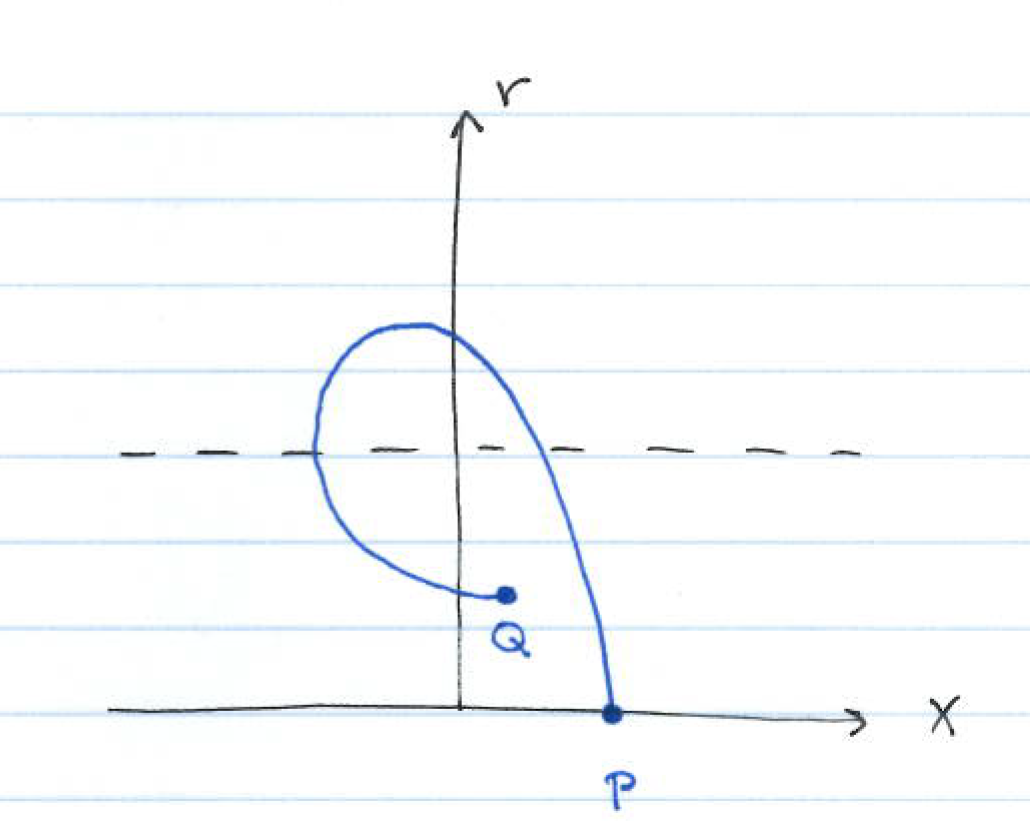
Figure 7. The shape of the geodesic $S[t]$ when $t>0$ is sufficiently small.

In order to do this, we need to understand the behavior of the geodesic $S[t]$ as it travels away from the $x$-axis, turns around, and travels back towards the $x$-axis. Following the proof in [16], we analyze $S[t]$ by writing it locally as graphs over the $r$-axis. The local graphical component $x=f(r)$ satisfies

(5.3) $$\frac{f^{\prime\prime}}{1+f^{\prime 2}}=\left(\frac{r}{2}-\frac{n-1}{r}\right)f^{\prime}-\frac{1}{2}f.$$

Taking a derivative of (5.3), we have

(5.4) $$\frac{f^{\prime\prime\prime}}{1+f^{\prime 2}}=\frac{2f^{\prime}(f^{\prime\prime})^{2}}{(1+f^{\prime 2})^{2}}+\left(\frac{r}{2}-\frac{n-1}{r}\right)f^{\prime\prime}+\frac{n-1}{r^{2}}f^{\prime}.$$

Notice that (5.4) is a second order differential equation for $f^{\prime}$ with positive coefficient on $f^{\prime}$. Much of the behavior of the geodesics $S[t]$ can be understood by analyzing these equations. We have the following results from [16]:

Proposition 7.

For $t>0$, let $f_{t}$ denote the solution to (5.3) with $f_{t}(0)=t$ and $f_{t}^{\prime}(0)=0$. Then $f_{t}^{\prime\prime}<0$, and there is a point $b_{t}>\sqrt{2(n-1)}$ so that $\lim_{r\to b_{t}}f^{\prime}_{t}(r)=-\infty$ and $f_{t}(b_{t})>-\infty$. Moreover, there exists $\tilde{t}>0$ so that if $t\in(0,\tilde{t}\,]$, then

$$b_{t}\geq\sqrt{\log{\frac{2}{\pi t^{2}}}},$$

$$\frac{-4(n+1)}{\sqrt{\log{\frac{2}{\pi t^{2}}}}}\leq f_{t}(b_{t})<0,$$

and $f_{t}(r)<0$, for $t\in(2\sqrt{n},b_{t}]$.

This proposition tells us that when $t>0$ is sufficiently small, the first component of $S[t]$ written as a graph over the $r$-axis is concave down, decreasing, and it crosses the $r$-axis, before it blows-up at the point $B_{t}=(f_{t}(b_{t}),b_{t})$. (Here, the graphical component blows-up in the sense that the tangent line at $B_{t}$ is orthogonal to the $r$-axis.)

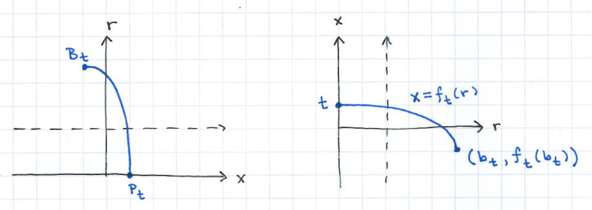
Figure 8. The initial shape of the first graphical component of $S[t]$ written as a graph over the $r$-axis when $0<t<\tilde{t}$.

In addition, Proposition 7 tells us $b_{t}\to\infty$ and $f_{t}(b_{t})\to 0$ as $t\to 0$. This behavior allows us to study the second component of $S[t]$ written as a graph over the $r$-axis when $t>0$ is sufficiently small.

Proposition 8.

Let $\tilde{t}>0$ be given as in the conclusion of Proposition 7. For $t\in(0,\tilde{t}\,]$, let $B_{t}=(f_{t}(b_{t}),b_{t})$, where $f_{t}$ is the solution to (5.3) with $f_{t}(0)=t$ and $f_{t}^{\prime}(0)=0$, and define $g_{t}$ to be the unique solution to (5.3) with $g_{t}(b_{t})=f_{t}(b_{t})$ and $\lim_{r\to b_{t}}g_{t}^{\prime}(r)=\infty$. Then there exists $0<\bar{t}<\tilde{t}$ so that for $t\in(0,\bar{t}\,]$, the solution $g_{t}$ has the following properties: there is $a_{t}\in(0,\sqrt{2(n-1)})$ so that $g_{t}$ is a maximally extended solution to (5.3) on the interval $(a_{t},b_{t})$; there is a point $c_{t}\in(a_{t},b_{t})$ so that $g_{t}^{\prime}(c_{t})=0$; $g_{t}^{\prime\prime}>0$; and $0<g_{t}(a_{t})<\infty$.

This proposition tells us that when $t>0$ is sufficiently small, the second component of $S[t]$ written as a graph over the $r$-axis is concave up, it crosses the $r$-axis, and it blows-up at the point $Q_{t}=(g_{t}(a_{t}),a_{t})$, where $0<a_{t}<\sqrt{2(n-1)}$ and $0<g_{t}(a_{t})<\infty$.

Figure 9. The initial shape of the second graphical component of $S[t]$ written as a graph over the $r$-axis when $0<t<\bar{t}$.

Combining these two propositions shows that $S[t]$ has the initial shape illustrated in Figure 7 when $0<t<\tilde{t}$.

Step 2: The second step is to increase the shooting parameter $t>0$ and show that there is $x_{*}\in(0,\sqrt{2n})$ so that $S[x_{*}]$ has the following shape:

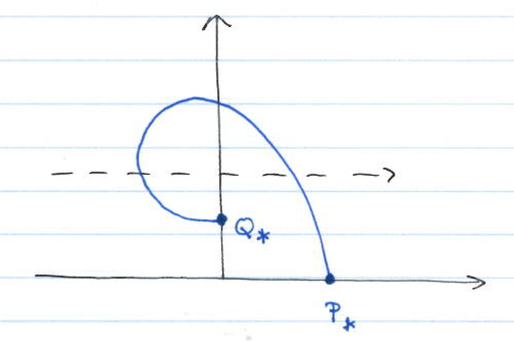
Figure 10. A sketch of the geodesic $S[x_{*}]$.

Using the notation from Step 1, we know that for $0<t\leq\bar{t}$, the geodesic $S[t]$ is strictly convex as it travels from $P_{t}=(t,0)$ to $B_{t}$ to $C_{t}$ to $Q_{t}$, and $Q_{t}$ lies in the same quadrant as $P_{t}$. We note that the the geodesic arc from $P_{t}$ to $Q_{t}$ is strictly convex in the sense that $(x^{\prime}r^{\prime\prime}-r^{\prime}x^{\prime\prime})$ is non-vanishing along the curve.

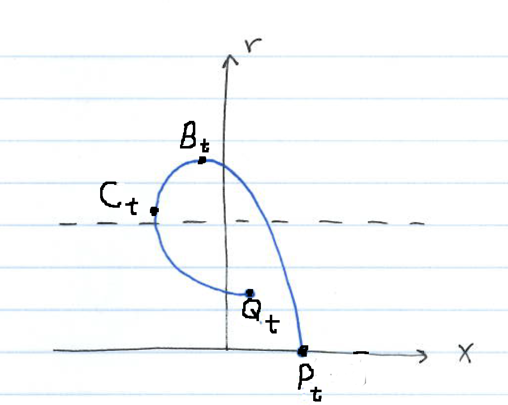
Figure 11. A geodesic arc $S[t]$ with property $\mathscr{P}(t)$.

To define the initial shooting coordinate $x_{*}$, we introduce the property $\mathscr{P}(t)$ for the geodesic $S[t]$. As in Figure 11, we say that $\mathscr{P}(t)$ holds if

• The geodesic $S[t]$ contains points $B_{t}$, $C_{t}$, and $Q_{t}$ as described in Step 1.

• The geodesic $S[t]$ is strictly convex as it travels from $P_{t}$ to $Q_{t}$.

• The geodesic $S[t]$ crosses the $r$-axis between $P_{t}$ and $B_{t}$ and then crosses back over between $C_{t}$ and $Q_{t}$.

We define the initial shooting coordinate $x_{*}$ by

(5.5) $$x_{*}=\sup\{x>0\,:\,\mathscr{P}(t)\textrm{ holds for all }t\in(0,x]\}.$$

It follows from Step 1 that $x_{*}$ is well-defined and $x_{*}\geq\bar{t}$.

By construction, for $0<t<x_{*}$, the geodesic $S[t]$ satisfies property $\mathscr{P}(t)$, and by continuous dependence on initial conditions, $S[t]$ converges to $S[x_{*}]$ as $t\uparrow x_{*}$. The following result summarizes the main properties of $S[x_{*}]$ established in [16].

Proposition 9.

Let $x_{*}$ be the initial shooting value defined in (5.5). Then

• $x_{*}<\sqrt{2n}$.

• As $t\uparrow x_{*}$, the points $B_{t}$, $C_{t}$, $Q_{t}$ on the geodesics $S[t]$ converge to distinct points $B_{x_{*}}$, $C_{x_{*}}$, $Q_{x_{*}}$ on $S[x_{*}]$ in a compact subset of $\mathbb{H}$.

• The geodesic $S[x_{*}]$ is strictly convex as it travels from $P_{x_{*}}$ to $Q_{x_{*}}$.

• The geodesic $S[x_{*}]$ crosses the $r$-axis between $P_{x_{*}}$ and $B_{x_{*}}$.

• The point $Q_{x_{*}}$ lies on the $r$-axis.

It follows from this proposition along with the symmetry of solutions to (5.1) with respect to reflections about the $r$-axis shows that $S[x_{*}]$ is the profile curve for an immersed $\mathbb{S}^{n}$ self-shrinker with the shape illustrated in Figure 3.

Remark 5.1.

In Step 2, the geodesic $S[x_{*}]$ is analyzed as the limit of the geodesics $S[t]$ as $t\uparrow x_{*}$. Now, each geodesic $S[t]$ is strictly convex as a curve from $P_{t}$ to $Q_{t}$. However, this does not imply that $S[x_{*}]$ is strictly convex. In fact, without further argument, we can only conclude that $S[x_{*}]$ is convex in the sense that $(x^{\prime}r^{\prime\prime}-r^{\prime}x^{\prime\prime})$ may vanish but does not change sign. There are indeed examples where the limiting geodesic may not be strictly convex. For instance, the geodesics $S[t]$ converge to the $r$-axis as $t\downarrow 0$. In the case of $S[x_{*}]$, proving the existence of the point $C_{x_{*}}$ ensures that $S[x_{*}]$ is strictly convex as it travels from $P_{x_{*}}$ to $Q_{x_{*}}$.

5.2. A collection of shooting problems for closed self-shrinkers

In this section, we sketch the behavior of geodesics for three shooting problems and illustrate how this behavior can be used to construct closed self-shrinkers. The analysis for the results stated in this section can be found in [20].

5.2.1. A second immersed sphere self-shrinker

Consider the shooting problem:

$$S[t]\textrm{ is the solution to~{}(\ref{SSEq}) with }S[t](0)=(t,0)\textrm{ and }S[t]^{\prime}(0)=(0,1).$$

For this shooting problem we consider the geodesics $S[t]$ when $t>0$ is close to 0. Given $N>0$, there exists $\varepsilon>0$ so that when $0<t<\varepsilon$, the geodesic $S[t]$ is strictly convex as it crosses back and forth over the $r$-axis with $N$ local maximums to the left of the $r$-axis and $N$ local minimums to the right of the $r$-axis.

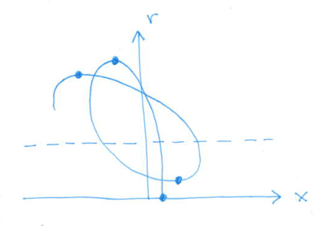
Figure 12. $S[t]$ for $t>0$ close to 0.

As was shown in the previous section, this shooting problem leads to the existence of the profile curve, $S[x_{*}]$, for an immersed $\mathbb{S}^{n}$ self-shrinker. We will sketch a proof that there is $x_{**}\in(0,x_{*})$ so that $S[x_{**}]$ is the profile curve for a second immersed $\mathbb{S}^{n}$ self-shrinker.

For $t$ close to $x_{*}$, the geodesic $S[t]$ has the following shape:

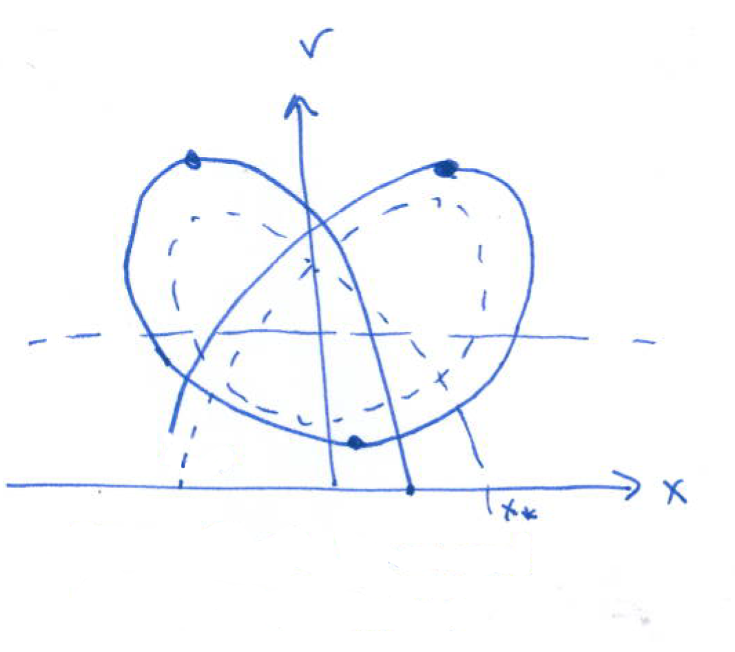
Figure 13. $S[t]$ for $t$ close to $x_{*}$.

Notice that the second local maximum points lie on different sides of the $r$-axis in the previous two figures. As $t$ varies from $0$ to $x_{*}$, a continuity argument can be used to show that there is $x_{**}\in(0,x_{*})$ so that the second local maximum lies on the $r$-axis. By the symmetry of geodesics with respect to reflections about the $r$-axis, $S[x_{**}]$ intersects the $x$-axis orthogonally at two points and is the profile curve for an immersed $\mathbb{S}^{n}$ self-shrinker.

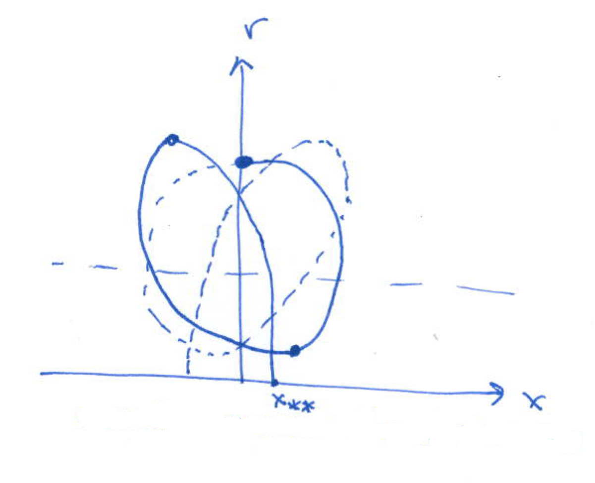
Figure 14. $S[x_{**}]$ is the profile curve for a second immersed $\mathbb{S}^{n}$ self-shrinker.

5.2.2. An embedded torus self-shrinker

Consider the shooting problem:

$$T[t]\textrm{ is the solution to~{}(\ref{SSEq}) with }T[t](0)=(0,t)\textrm{ and }T[t]^{\prime}(0)=(1,0).$$

For this shooting problem we consider the geodesics $T[t]$ when $t>0$ is close to 0. Solutions to this shooting problem behave similarly to solutions from the previous shooting problem, maintaining their strict convexity as they cross back and forth over the $r$-axis with local maximums to the left of the $r$-axis and local minimums (for $s>0$) to the right of the $r$-axis.

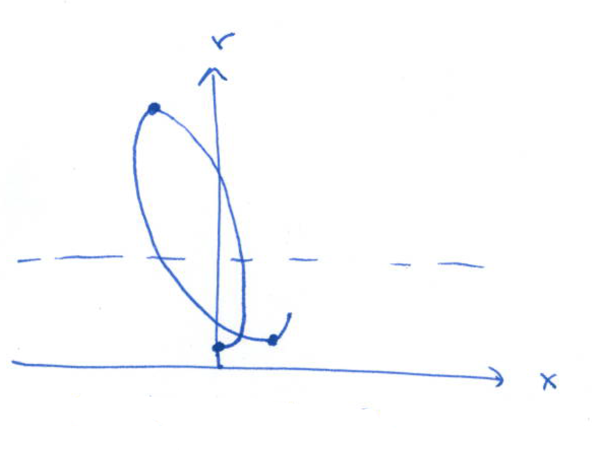
Figure 15. $T[t]$ for $t>0$ close to 0.

Increasing $t$ away from $0$ leads to the profile curve for an immersed $\mathbb{S}^{n}$ self-shrinker with the shape illustrated in Figure 3. In particular, we have two convex geodesic arcs with local maximums on opposite sides of the $r$-axis. A continuity argument can be used to show that there is a simple closed strictly convex geodesic that intersects the $r$-axis orthogonally at two points. Such a geodesic is the profile curve of an $\mathbb{S}^{1}\times\mathbb{S}^{n-1}$ self-shrinker.

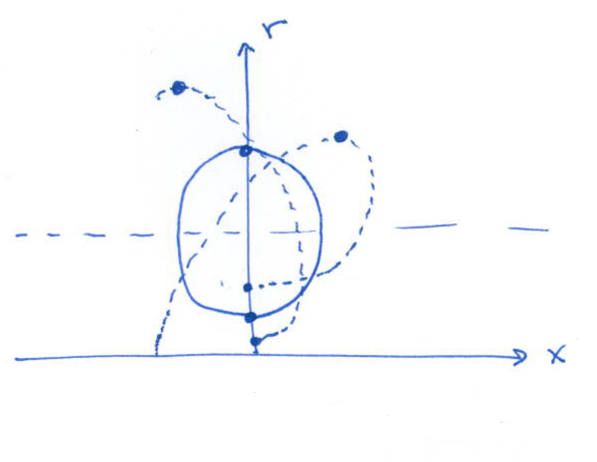
Figure 16. The profile curve of an embedded $\mathbb{S}^{1}\times\mathbb{S}^{n-1}$ self-shrinker.

5.2.3. An immersed torus self-shrinker

Consider the shooting problem:

$$T[t]\textrm{ is the solution to~{}(\ref{SSEq}) with }T[t](0)=(0,t)\textrm{ and }S[t]^{\prime}(0)=(1,0).$$

For this shooting problem we consider the geodesics $T[t]$ when $t<\sqrt{2(n-1)}$ is close to $\sqrt{2(n-1)}$. Solutions to this shooting problem cross back and forth over the geodesic $r\equiv\sqrt{2(n-1)}$ oscillating in a shape that resembles $\infty$:

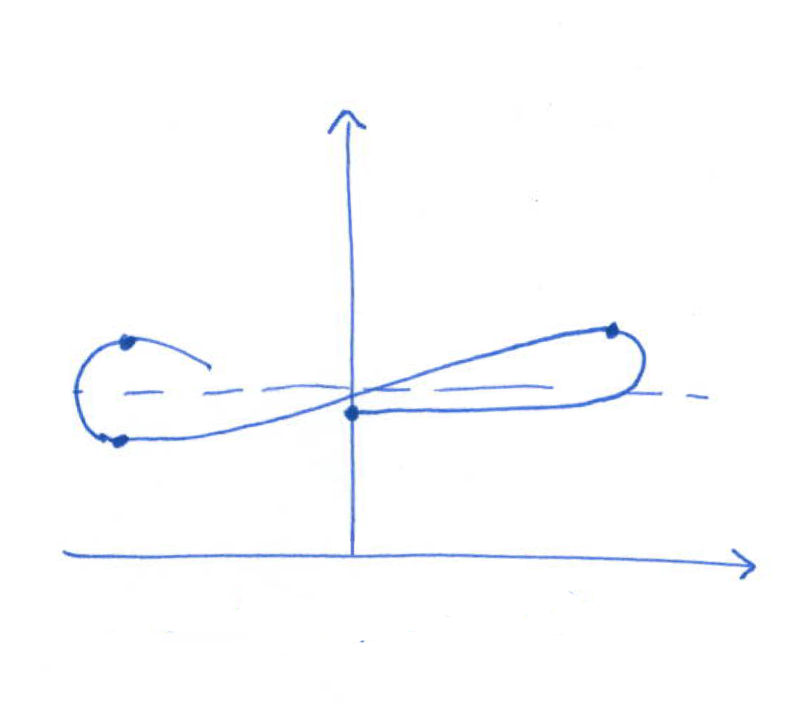
Figure 17.

Decreasing $t$ away from $\sqrt{2(n-1)}$ again leads to the profile curve for an immersed $\mathbb{S}^{n}$ self-shrinker with the shape illustrated in Figure 3. In particular, right before $t$ reaches this profile curve, $T[t]$ has the following shape:

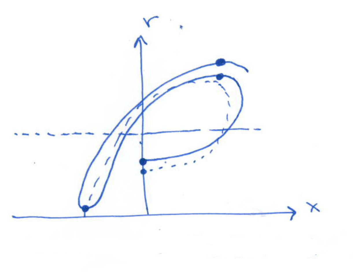
Figure 18.

Comparing the geodesic arcs in the previous two figures, we see that the second local maximum points lie on opposite sides of the $r$-axis. It follows that there is $r_{*}\in(0,\sqrt{2(n-1)})$ so that $T[r_{*}]$ intersects the $r$-axis orthogonally at two points:

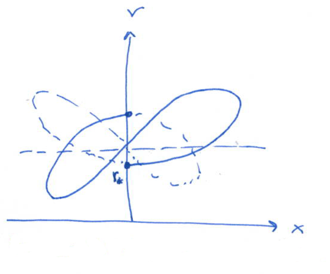
Figure 19. $T[r_{*}]$ is the profile curve for an immersed $\mathbb{S}^{1}\times\mathbb{S}^{n-1}$ self-shrinker.

5.3. The role of continuity in the shooting method

In this section we discuss the role of continuity in the shooting method for constructing closed geodesics in $(\mathbb{H},g_{Ang})$. First of all, since the shooting method is implemented by varying the initial position and velocity for solutions to (5.2), the continuous dependence of solutions on initial conditions is the main force at work. Next, we observe that the geodesic equation (5.1), re-written as

$$\frac{x^{\prime}r^{\prime\prime}-x^{\prime\prime}r^{\prime}}{(x^{\prime 2}+r^{\prime 2})^{3/2}}=\left(\frac{n-1}{r}-\frac{r}{2}\right)\frac{x^{\prime}}{\sqrt{x^{\prime 2}+r^{\prime 2}}}+\frac{1}{2}x\frac{r^{\prime}}{\sqrt{x^{\prime 2}+r^{\prime 2}}},$$

gives uniform bounds for the Euclidean curvature of geodesic arcs in a fixed compact subset of $\mathbb{H}$. This tells us that as we vary the initial conditions in the shooting problem, the limit of geodesic arcs in a fixed compact subset of $\mathbb{H}$ will not develop corners or collapse onto a curve with multiplicity. (We note that this type of behavior does occur at the boundary of $\mathbb{H}$ when geodesics converge to half-entire graphs with multiplicity [20]).

Now, the geodesic equation (5.1) is symmetric with respect to reflections across the $r$-axis, so the existence of a closed geodesic can be established by finding a geodesic arc that intersects the $r$-axis orthogonally at two points. One way to find such a geodesic arc is to build a framework where the following three properties hold:

1. There is a point $P_{1}$ so that the geodesic arc obtained from shooting orthogonally to the $r$-axis at $P_{1}$ with tangent angle 0 contains a point $Q_{1}$, located to the left of the $r$-axis with tangent angle $\pi$.

   

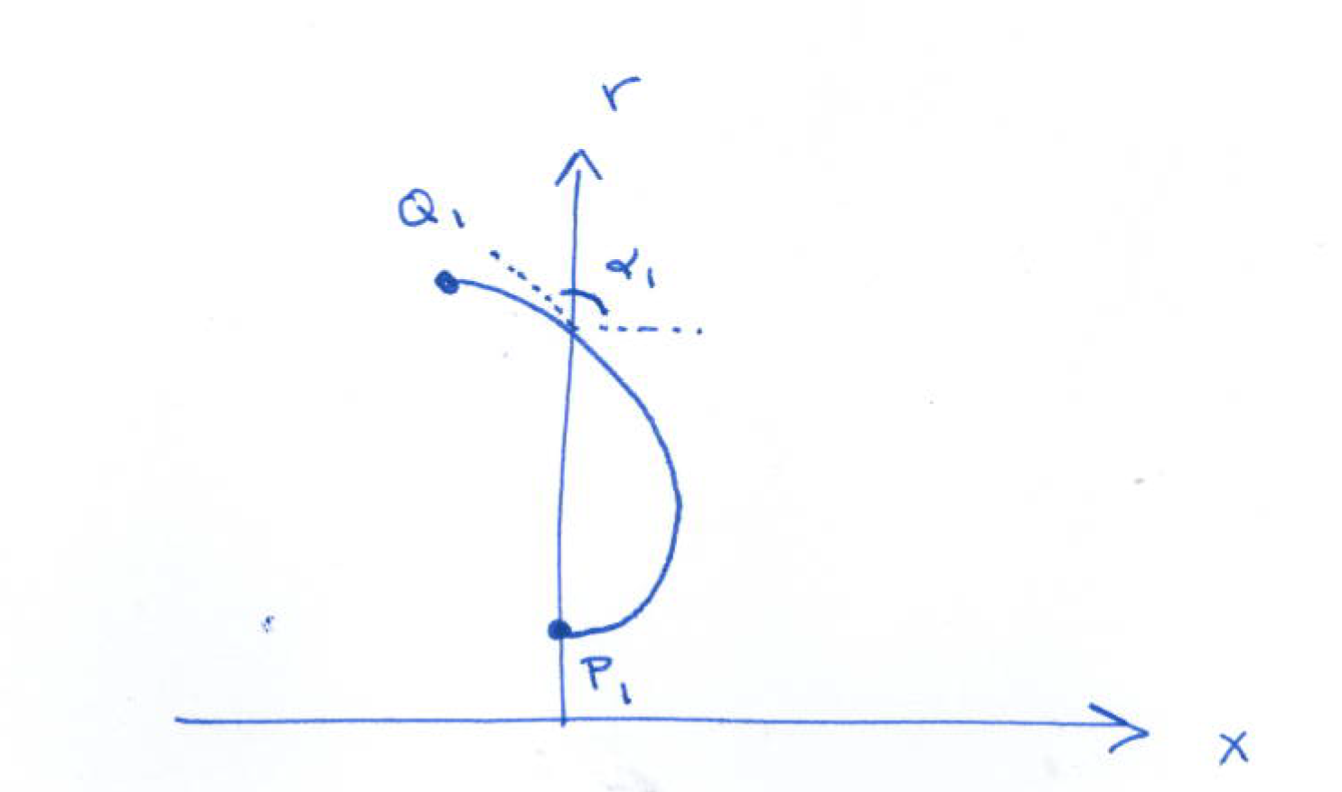
   Figure 20.

2. There is a point $P_{2}$ so that the geodesic arc obtained from shooting orthogonally to the $r$-axis at $P_{2}$ with tangent angle 0 contains a point $Q_{2}$, located to the right of the $r$-axis with tangent angle $\pi$.

   

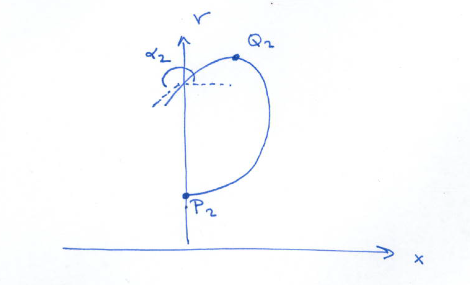
   Figure 21.

3. For each point $P$ on the $r$-axis, between $P_{1}$ and $P_{2}$, the geodesic arc obtained from shooting orthogonally to the $r$-axis at $P$ with tangent angle 0 travels from $P$ to a point $Q$ with tangent angle $\pi$. In addition, as $P$ varies from $P_{1}$ to $P_{2}$, the geodesic arcs connecting $P$ to $Q$ vary smoothly and remain inside a compact subset of $\mathbb{H}$. (We note that under these assumptions, (5.1) implies that the geodesics are strictly convex at $Q$).

Remark 5.2.

In this example, continuity, combined with the behavior of the geodesic arcs through $P_{1}$ and $P_{2}$, guarantees that there is a point $P_{*}$ on the $r$-axis (between $P_{1}$ and $P_{2}$) so that the geodesic arc from $P_{*}$ to $Q_{*}$ intersects the $r$-axis orthogonally at $Q_{*}$. Notice how the third property is stated to ensure that continuity can be applied to the problem. For a shooting problem like this, the existence of the points $Q$ needs to be established as continuous dependence on initial conditions does not guarantee that the orthogonal tangent lines (tangent angle $\pi$) will be preserved as $P$ varies.

Remark 5.3.

As an alternative to tracking the points $Q$ as $P$ varies from $P_{1}$ to $P_{2}$, the crossing angles $\alpha$, where the geodesic arc meets the $r$-axis could be studied instead. In the above illustrations, $\alpha_{1}$ is less than $\pi$ and $\alpha_{2}$ is greater than $\pi$. In this case, if the crossing points exist, the crossing angles vary continuously, and the geodesic arcs remain in a compact subset of the domain, then there is a geodesic arc that intersects the $r$-axis with a crossing angle of $\pi$.

6. Self-shrinkers with bi-rotational symmetry

In this section, we consider the problem of constructing closed self-shrinkers with bi-rotational symmetry. A hypersurface in $\mathbb{R}^{M_{1}+M_{2}+2}$ has bi-rotational symmetry if it can be written in the form

$$\mathbf{X}(s,p_{1},p_{1})=\left(x(s){\mathbf{p}_{1}},y(s){\mathbf{p}_{2}}\right),$$

where $(x(s),y(s))$ is a curve in the positive quadrant $\mathcal{Q}=\{(x,y)\in\mathbb{R}^{2}\,|\,x>0,y>0\}$, ${\mathbf{p}_{1}}\in{\mathbb{S}}^{M_{1}}$, ${\mathbf{p}_{2}}\in{\mathbb{S}}^{M_{2}}$, and $M_{1}$ and $M_{2}$ are positive integers.

Historically, bi-rotational symmetry has produced rich examples of solutions to classical problems. Hsiang [34] proved the existence of infinitely many distinct bi-rotational CMC immersions of ${\mathbb{S}}^{N-1}$ in ${\mathbb{R}}^{N\geq 4}$. These examples show that Hopf’s Theorem does not extend to higher dimensions. Alencar-Barros-Palmas-Reyes-Santo [4, Theorem 1.2] proved the existence of various bi-rotational minimal hypersurfaces in ${\mathbb{R}}^{M_{1}+M_{2}+2\geq 8}$ with $M_{1},M_{2}\geq 2$, that are asymptotic or doubly asymptotic to the minimal Clifford cone. Bombieri-De Giorgi-Giusti [10, Section IV] investigated bi-radial graphs of the form $x_{2m+1}=F(\sqrt{{x_{1}}^{2}+\cdots+{x_{m}}^{2}\,},\sqrt{{x_{m+1}}^{2}+\cdots+{x_{2m}}^{2}})$. They proved the existence of an entire, non-flat minimal graph in $\mathbb{R}^{9}$, which showed that Bernstein’s Theorem does not hold in $\mathbb{R}^{N\geq 9}$. Recently, Del Pino-Kowalczyk-Wei [15] studied the asymptotic behavior of the Bombieri-De Giorgi-Giusti graph and proved the existence of a counterexample to De Giorgi’s conjecture for the Allen-Cahn equation in $\mathbb{R}^{N\geq 9}$.

The following reduction tells us that the profile curve of a bi-rotational self-shrinker is a weighted geodesic in $\mathcal{Q}$.

Proposition 10 (Bi-rotational self-shrinkers from weighted geodesics in $\mathcal{Q}$).

Let $\alpha<0$ be a constant, let $M_{1}$ and $M_{2}$ be positive integers, and let $\gamma(s)=(x(s),y(s))$, $s\in I$, be an immersed curve in the positive quadrant $\mathcal{Q}$. The following conditions are equivalent.

• The bi-rotational hypersurface

  $${\Sigma}^{M_{1}+M_{2}+1}=\left\{\;\mathbf{X}=(x(s){\mathbf{p}_{1}},y(s){\mathbf{p}_{2}})\in{\mathbb{R}}^{M_{1}+M_{2}+2}\;\;|\;\;s\in I,\;{\mathbf{p}_{1}}\in{\mathbb{S}}^{M_{1}},\;{\mathbf{p}_{2}}\in{\mathbb{S}}^{M_{2}}\;\right\}$$

  is a self-shrinker, satisfying ${\Delta}_{{\mathbf{g}}_{{}_{\Sigma}}}\mathbf{X}=\alpha\mathbf{X}^{\bot}$.

• The profile curve $\gamma(s)=(x(s),y(s))$ is a weighted geodesic in the positive quadrant $\mathcal{Q}$ equipped with the density

  $$x^{M_{1}}y^{M_{2}}e^{\,\alpha\frac{x^{2}+y^{2}}{2}}.$$

• The profile curve $\gamma(s)=(x(s),y(s))$ satisfies the geodesic equation

  (6.1) $$\frac{x^{\prime}y^{\prime\prime}-x^{\prime\prime}y^{\prime}}{x^{\prime 2}+y^{\prime 2}}=-\left(\frac{M_{1}}{x}+\alpha x\right)y^{\prime}+\left(\frac{M_{2}}{y}+\alpha y\right)x^{\prime}.$$

As in the rotational symmetry case, the shooting method can be used to explore profile curves of bi-rotational self-shrinkers, and the existence of a closed self-shrinker with bi-rotational symmetry is equivalent to finding a solution to (6.1) that is closed or intersects the boundary of $\mathcal{Q}$ orthogonally at two points.

6.1. The shooting method for bi-rotational self-shrinkers

In this section we adopt the normalization $\alpha=-\frac{1}{2}$, and we make the additional assumption that $M_{1}=M_{2}=M\geq 1$. Then, the geodesic equation (6.1) becomes

(6.2) $$\frac{x^{\prime}y^{\prime\prime}-x^{\prime\prime}y^{\prime}}{x^{\prime 2}+y^{\prime 2}}=-\left(\frac{M}{x}-\frac{1}{2}x\right)y^{\prime}+\left(\frac{M}{y}-\frac{1}{2}y\right)x^{\prime}.$$

Notice that for a geodesic $y=y(x)$ written as a graph over the $x$-axis, we have the following equation which resembles equation (5.3) for self-shrinkers with rotational symmetry:

(6.3) $$\frac{y^{\prime\prime}}{1+y^{\prime 2}}=-\left(\frac{M}{x}-\frac{1}{2}x\right)y^{\prime}+\left(\frac{M}{y}-\frac{1}{2}y\right).$$

Examples of bi-rotational self-shrinkers in ${\mathbb{R}}^{2M+2}$ include the minimal Clifford cone, round cylinders $\mathbb{S}^{M}\times\mathbb{R}^{M+1}$ of radius $\sqrt{2M\,}$ with ‘axis’ through the origin, and the round sphere of radius $\sqrt{2(2M+1)}$ centered at the origin. We have the following profile curves for these examples:

• Minimal Clifford cone: $y=x$,

• Round cylinders: $y=\sqrt{2M\,}$ and $x=\sqrt{2M\,}$,

• Round sphere: $x^{2}+y^{2}=2(2M+1)$.

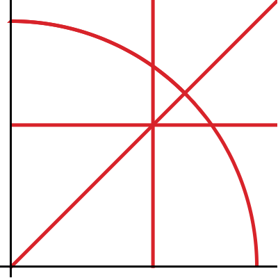
Figure 22. Geodesics corresponding to the Clifford cone, two round cylinders, and the round sphere.

The assumption $M_{1}=M_{2}=M$ introduces an additional symmetry as the geodesic equation (6.2) is now symmetric with respect to reflections about the line $y=x$. Consequently, a closed geodesic can be constructed by finding a geodesic arc that intersects the line $y=x$ orthogonally at two points.

Reparametrizing a solution to (6.2) so that the curve satisfies $x^{\prime}(s)^{2}+y^{\prime}(s)^{2}=1$, shows that the tangent angle $\alpha(s)$ is a solution to the system

(6.4) $$\left\{\begin{array}[]{lll}x^{\prime}(s)&=&\cos\alpha(s),\\ y^{\prime}(s)&=&\sin\alpha(s),\\ \alpha^{\prime}(s)&=&-\left(\frac{M_{1}}{x(s)}-\frac{x(s)}{2}\right)\sin\alpha(s)+\left(\frac{M_{2}}{y(s)}-\frac{y(s)}{2}\right)\cos\alpha(s).\end{array}\right.$$

This leads to the shooting problem:

(6.5) $$T[t]\textrm{ is the solution to~{}(\ref{bi:SSEq}) with }T[t](0)=(t,t)\textrm{ and }T[t]^{\prime}(0)=\left(-\frac{1}{\sqrt{2}},\frac{1}{\sqrt{2}}\right).$$

As described in Section 5.3, the existence of a closed geodesic can be established by showing that the above shooting problem exhibits the two types of behavior illustrated in Figure 23.

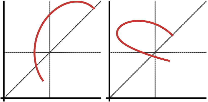
Figure 23.

McGrath has posted a preprint [47] which shows that $T[t]$ exhibits the behavior illustrated on the left of Figure 23, for large values of the parameter $t$. In this preprint, McGrath presents a shooting method argument similar to the ones used to construct closed self-shrinkers with rotational symmetry in [9] and [16]. The approach is to analyze the geodesics $T[t]$ as $t$ decreases from $\infty$ and deduce through continuity that $T[t_{*}]$ is a closed geodesic for some $t_{*}>0$. We note that the presence of the additional term in (6.2), when compared to (5.1), makes the analysis of bi-rotational geodesics more complicated than their rotational counterparts.

6.2. Numerical approximations for profile curves of bi-rotational self-shrinkers in ${\mathbb{R}}^{4}$

In this section we present numerical approximations of symmetric profile curves for closed self-shrinkers with bi-rotational symmetry in the case where $\alpha=-\frac{1}{2}$ and $M_{1}=M_{2}=1$. We used Wolfram Mathematica to plot numerical solutions to the system (6.4) for various initial values in the shooting problem (6.5).

1. Embedded ${\mathbb{T}}^{3}$ self-shrinker in ${\mathbb{R}}^{4}$: A detailed analysis of (6.3), adapted from the crossing arguments in [16] and [20], confirms there is a $t_{2}>0$ so that the geodesic $T[t]$ has the initial shape illustrated on the left of Figure 23 for $t\geq t_{2}$. Numerics show that there is a $t_{1}>\sqrt{6}$ so that $T[t_{1}]$ has the following initial shape:

   

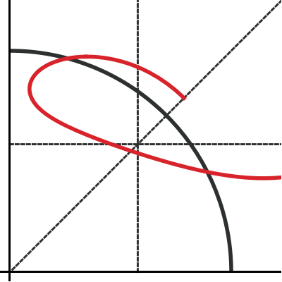
   Figure 24.

   The framework of Remark 5.3 can now be implemented to prove the existence of a simple, closed geodesic. However, as discussed in Section 5.3, additional details on the behavior of the geodesics $T[t]$, $t\in[t_{1},t_{2}]$ are needed to run the continuity argument, and the existence of a geodesic with the shape of $T[t_{1}]$ in Figure 24 still needs to be established. Here is a numerical approximation of a simple, closed geodesic:

   

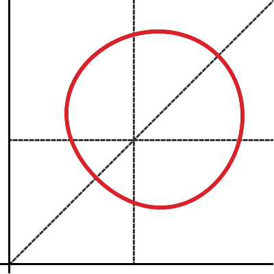
   Figure 25.

   
   

2. Three immersed ${\mathbb{T}}^{3}$ self-shrinkers in ${\mathbb{R}}^{4}$:

   

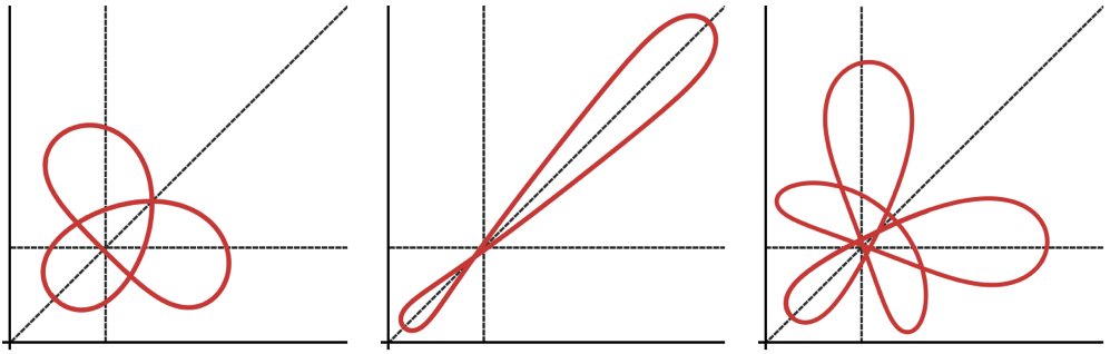
   Figure 26.

   
   

3. Two immersed ${\mathbb{S}}^{3}$ self-shrinkers in ${\mathbb{R}}^{4}$:

   

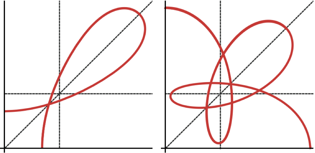
   Figure 27.

7. Open Problems

We end the survey with a list of open problems for closed self-shrinkers. One may also raise similar questions for the existence and uniqueness of closed self-shrinkers in higher dimensions.

Open Problem 1.

Is Angenet’s rotational torus the only closed, embedded, genus 1 self-shrinker in $\mathbb{R}^{3}$?

The uniqueness of Angenent’s torus is even unknown in the class of self-shrinkers with rotational symmetry. The embeddedness assumption is necessary due to the immersed examples constructed in [20]. Very recently, motivated by Lawson’s Theorem [45] for embedded minimal surfaces in the three-dimensional sphere, Mramor and Wang [51, Corollary 1.2] exploited the variational characterization of self-shrinkers (Section 2.4) to show that an embedded self shrinking torus in $\mathbb{R}^{3}$ is un-knotted.

Open Problem 2.

Is the round sphere centered at the origin the only embedded $\mathbb{S}^{3}$ self-shrinker in $\mathbb{R}^{4}$?

The embeddedness assumption is necessary due to the existence of immersed and non-embedded $\mathbb{S}^{3}$ self-shinkers constructed in [16, 20]. Uniqueness is known in the rotational case [17, 43].

Open Problem 3.

Existence and uniqueness of closed self-shrinkers with bi-rotational symmetry.

Are there bi-rotational self-shrinkers for the numeric profile curves presented in Section 6.2? Are there any uniqueness results for these or other bi-rotational examples?

References

- [1] U. Abresch, J. Langer, The normalized curved shortening flow and homothetic solutions, J. Differential Geom. 23 (1986), 175–196.
- [2] U. Abresch, Constant mean curvature tori in terms of elliptic functions, J. Reine Angew. Math. 374 (1987), 169–192.
- [3] U. Abresch. H. Rosenberg, A Hopf differential for constant mean curvature surfaces in and , Acta Math. 193 (2004), no. 2, 141–174.
- [4] H. Alencar, A. Barros, O. Palmas, J. G. Reyes, W. Santos, -invariant minimal hypersurfaces in , Ann. Global Anal. Geom. 27 (2005), 179–199.
- [5] B. Andrews, P. Bryan, A comparison theorem for the isoperimetric profile under curve-shortening flow, Comm. Anal. Geom. 19 (2011), no. 3, 503–539.
- [6] B. Andrews, P. Bryan, Curvature bound for curve shortening flow via distance comparison and a direct proof of Grayson’s theorem, J. Reine Angew. Math. 653 (2011), 179–187.
- [7] S. Angenent, Parabolic equations for curves on surfaces. I. Curves with -integrable curvature, Ann. of Math. (2), 132 (1990), 451–483.
- [8] S. Angenent Parabolic equations for curves on surfaces. II. Intersections, blow-up and generalized solutions, Ann. of Math. (2), 133 (1991), 171–215.
- [9] S. Angenent, Shrinking doughnuts, Nonlinear diffusion equations and their equilibrium states, 3 (Gregynog, 1989), 21–38, Progr. Nonlinear Differential Equations Appl. 7, Birkhäuser, Boston, 1992.
- [10] E. Bombieri, E. De Giorgi, E. Giusti, Minimal cones and the Bernstein problem, Invent. Math. 7 (1969), 243–268.
- [11] R. L. Bryant, Complex analysis and a class of Weingarten surfaces, arXiv preprint arXiv:1105.5589 (2011).
- [12] S. Brendle, Embedded self-similar shrinkers of genus , Annals of Math. 183 (2016), 715–728.
- [13] J.-E. Chang, One dimensional solutions of the -self shrinkers, Geom. Dedicata. 189 (2017), 97–112.
- [14] T. H. Colding, W. P. Minicozzi II, E. K. Pedersen, Mean curvature flow, Bull. Amer. Math. Soc. (N.S.) 52 (2015), no. 2, 297–333.
- [15] M. del Pino, M. Kowalczyk, J. Wei, On De Giorgi’s conjecture in dimension , Ann. of Math. (2) 174 (2011), no. 3, 1485–1569.
- [16] G. Drugan, An immersed self-shrinker, Trans. Amer. Math. Soc. 367 (2015), no. 5, 3139–3159.
- [17] G. Drugan, Self-shrinking solutions to mean curvature flow. Ph.D. thesis, University of Washington, 2014.
- [18] G. Drugan, X. H. Nguyen, Mean curvature flow of entire graphs evolving away from the heat flow, Proc. Amer. Math. Soc. 145 (2017), no. 2, 861–869.
- [19] G. Drugan, X. H. Nguyen, Shrinking doughnuts via variational methods, arXiv preprint arXiv:1708.08808 (2017).
- [20] G. Drugan, S. J. Kleene, Immersed self-shrinkers, Trans. Amer. Math. Soc. 369 (2017), no. 10, 7213–7250.
- [21] K. Ecker, Regularity theory for mean curvature flow, Progress in Nonlinear Differential Equations and their Applications, 57. Birkhäuser, Boston, Inc., Boston, MA, 2004.
- [22] C. L. Epstein, M. I. Weinstein, A stable manifold theorem for curve shortening equations, Comm. Pure Appl. Math. 40 (1987), no. 1, 119–139.
- [23] A. Fraser, R. Schoen, Uniqueness theorems for free boundary minimal disks in space forms, Int. Math. Res. Not. 2015, no. 17, 8268–8274.
- [24] M. Gage, Deforming curves on convex surfaces to simple closed geodesics, Indiana Univ. Math. J. 39 (1990), 1037–1059.
- [25] M. Gage, R. S. Hamilton, The heat equation shrinking convex plane curves, J. Differential Geom. 23 (1986), 69–96.
- [26] V. Gimeno, Isoperimetric inequalities for submanifolds. Jellett-Minkowski’s formula revisited, Proc. Lond. Math. Soc. (3) 110 (2015), no. 3, 593–614.
- [27] M. A. Grayson, The heat equation shrinks embedded plane curves to round points, J. Differential Geom. 26 (1987), 285–314.
- [28] H. P. Halldorsson, Self-similar solutions to the curve shortening flow, Trans. Amer. Math. Soc. 364 (2012), no. 10, 5285–5309.
- [29] H. P. Halldorsson, Self-similar solutions to the mean curvature flow in the Minkowski plane , J. Reine Angew. Math. 704 (2015), 209–243.
- [30] R. S. Hamilton, Monotonicity formulas for parabolic flows on manifolds, Comm. Anal. Geom. 1 (1993), no 1. 127–137.
- [31] H. Hopf, Differential geometry in the large: seminar lectures New York University 1946 and Stanford University 1956. Vol. 1000. Springer, 2003.
- [32] D. Hoffman, The computer-aided discovery of new embedded minimal surfaces, Math. Intelligencer, 9 (1987), no. 3, 8–21.
- [33] W. Y. Hsiang, Z. H. Teng, W.C. Yu, New examples of constant mean curvature immersions of spheres into Euclidean space, Ann. of Math. 117 (1983), no. 3, 609–625.
- [34] W. Y. Hsiang, Generalized rotational hypersurfaces of constant mean curvature in the Euclidean spaces. I. J. Differential Geom. 17 (1982), no. 2, 337–356.
- [35] C. C. Hsiung, Some integral formulas for closed hypersurfaces in Riemannian space, Pacific J. Math. 6 (1956), 291–299.
- [36] C. C. Hsiung, Some integral formulas for closed hypersurfaces, Math. Scand. 2 (1959), 286–294.
- [37] G. Huisken, Flow by mean curvature of convex surfaces into spheres, J. Differential Geom. 20 (1984), no. 1, 237–266.
- [38] G. Huisken, Asymptotic behavior for singularities of the mean curvature flow, J. Differential Geom. 31 (1990), no. 1, 285–299.
- [39] G. Huisken, A distance comparison principle for evolving curves, Asian J. Math. 2 (1998), no. 1, 127–133.
- [40] Ilmanen, Lectures on Mean Curvature Flow and Related Equations, 1998.
- [41] N. Kapouleas, S. J. Kleene, N. M. Møller, Mean curvature self-shrinkers of high genus: non-compact examples, arXiv preprint arXiv:1106.5454 (2011), to appear in J. Reine Angew. Math.
- [42] K. Kenmotsu, Weierstrass formula for surfaces of prescribed mean curvature, Math. Ann. 245 (1979), no. 2, 89–99.
- [43] S. J. Kleene, N. M. Møller, Self-shrinkers with a rotational symmetry, Trans. Amer. Math. Soc. 366 (2014), no. 8, 3943–3963.
- [44] K.-K. Kwong, An extension of Hsiung-Minkowski formulas and some applications, J. Geom. Anal. 26 (2016), no. 1, 1–23.
- [45] H. B. Lawson, The unknottedness of minimal embeddings, Invent. Math. 11 (1970), 183–187.
- [46] A. Magni, C. Mantegazza, A note on Grayson’s theorem, Rend. Semin. Mat. Univ. Padova, 131 (2014), 263–279.
- [47] P. McGrath, Closed mean curvature self-shrinking surfaces of generalized rotational type, arXiv preprint arXiv:1507.00681 (2015).
- [48] F. Morgan, Geometric Measure Theory. A Beginner’s Guide, fourth ed. Elsevier/Academic Press, Amsterdam, 2009.
- [49] N. M. Møller, Closed self-shrinking surfaces in via the torus, arXiv preprint arXiv:1111.7318 (2011).
- [50] S. Montiel, Unicity of constant mean curvature hypersurfaces in some Riemannian manifolds, Indiana Univ. Math. J. 48 (1999), no. 2, 711–748.
- [51] A. Mramor, S. Wang, On the topological rigidity of compact self shrinkers in , arXiv preprint arXiv:1708.06581 (2017).
- [52] W. W. Mullins, Two Dimensional Motion of Idealized Grain Boundaries, Journal of Applied Physics, 27 (1956), no. 8, 900–904.
- [53] H. Wente, Counterexample to a conjecture of H. Hopf, Pacific J. Math. 121 (1986), no. 1, 193–243.