Abstract

We study single spin asymmetries at one-loop accuracy in semi-inclusive DIS with a transversely polarized hadron in the initial state. Two measurable spin observables are predicted in the framework of QCD collinear factorization. One of the spin observables is the Sivers weighted asymmetry, another one is the Collins weighted asymmetry. The prediction takes a form of convolutions of perturbative coefficient functions and nonperturbative functions, which are twist-2 transversity distributions, twist-3 parton distributions, twist-2- and twist-3 parton fragmentation functions. These nonperturbative functions can be extracted from measurements of the spin observables and provide valuable information of the inner structure of hadrons. The measurements can be done in current COMPASS- and JLab experiments and in future experiments of EIC. The perturbative coefficient functions are calculated at one-loop level. There are collinear divergences in the calculation involving chirality-even- and chirality-odd twist operators. We find that all collinear divergences can be correctly subtracted so that the final results are finite.

1. Introduction

Experiments of lepton-hadron scattering have provided important information about the inner structure of hadrons. A typical example is Deeply Inelastic Scattering(DIS). From DIS one can extract parton distribution functions defined with twist-2 operators of QCD. In Semi-Inclusive DIS(SIDIS) with one detected hadron in the final state, one can learn more about the inner structure and nonperturbative properties of QCD, if the initial hadron is transversely polarized. In this case the spin-dependent part of the differential cross-section, or Single-Spin Asymmetries(SSA’s), can be predicted with parton distributions defined with twist-3 operators as shown in [1, 2], and twist-3 Fragmentation Functions(FF’s). The twist-3 parton distributions describe quark-gluon correlations inside a hadron and contain more information about the inner structure of hadrons than twist-2 parton distributions. In this work, we study SSA’s in SIDIS, in particular one-loop corrections of spin-observables.

Under one-photon-exchange approximation, the hadronic tensor of SIDIS contains all information about the process. The spin-dependent part of the tensor has been studied with collinear factorization at tree-level in different kinematic regions. In the region where the final hadron has large transverse momentum $P_{h\perp}$, SSA has been studied in [3, 4, 5], where the spin-dependent part starts at order of $\alpha_{s}$. At low $P_{h\perp}$ one can also employ collinear factorization because of the large virtuality $-Q^{2}$ of the exchanged photon. In this region, the spin-dependent part starting at order of $\alpha_{s}^{0}$ is predicted as a tensor distribution of $P_{h\perp}$ as shown in [9]. This implies that the measurable effects from this part can only be predicted when $P_{h\perp}$ is integrated over with certain weights. In this work we construct two spin-observables by integrating over $P_{h\perp}$ with different weights, and study one-loop corrections of the two spin-observables.

Various SSA’s in SIDIS can be measured in current experiment of COMPASS[6] and JLab[7] and in future experiment of EIC[8]. It is noted in the low $P_{h\perp}$ region one can employ the approach of Transverse-Momentum-Dependent(TMD) factorization studied in [10, 11, 12], where nonperturbative effects are described by TMD parton distributions and TMD FF’s. The relevant phenomenology with TMD factorization for SIDIS has been studied in [13, 14, 15, 16]. In the framework of TMD factorization, the SSA related to Sivers function, which is one of TMD parton distributions, is called Sivers Asymmetry. The SSA related to Collins fragmentation function is called Collins asymmetry. These two asymmetries have already been studied in experiment by HERMES and COMPASS. It is found that these asymmetries are different than zero[17, 18]. Recently, the so-called weighted Sivers asymmetry has been studied by COMPASS[19]. One of our two spin observables is in fact the studied weighted Sivers asymmetry. Another one is the weighted Collins asymmetry, because it is related to the transverse momentum moment of Collins fragmentation function. These two asymmetries have important implications, if they are not zero. If Sivers asymmetry is not zero, it indicates that partons inside a hadron have nonzero orbital angular momentum. Nonzero Collins asymmetry indicates that partons in their fragmentation into a hadron can have nonzero orbital angular momentum.

Without observing the spin of the final hadron, twist-3 contributions only appear in the case when the initial hadron is transversely polarized. The spin-dependent part of the hadronic tensor can obtain contributions from twist-3 parton distributions introduced in [1, 2] combined with twist-2 quark FF. These twist-3 parton distributions and twist-2 FF are defined with chirality-even operators. We will call these contributions as chirality-even contributions. Besides them the spin-dependent part also receives contributions from the twist-2 transversity distribution introduced in [20], combined with twist-3 FF’s. The transversity distribution and twist-3 FF’s are defined with chirality-odd operators. We will call these contributions as chirality-odd contributions. At the leading order of $\alpha_{s}$, i.e., at $\alpha_{s}^{0}$, one of our two spin observables has only a chirality-even contributions, while another has only a chirality-odd contribution. Therefore, through the two observables one can extract not only twist-3 parton distributions and fragmentation functions, but also the twist-2 transversity distribution, which is less known than other twist-2 parton distributions. Beyond tree-level, each spin observable can have chirality-even- and chirality-odd contributions.

It is worth to point out that there are not many results of one-loop calculation involving twist-3 operators, while calculations beyond tree-level with only twist-2 operators are rather standard and many one-loop results exist. For Drell-Yan processes with one transversely polarized hadron in the initial state, one-loop correction of a spin observable involving the twist-3 parton distributions is calculated at one-loop in [21]. In [22] two spin observables are studied and their complete one-loop corrections are derived. For SIDIS, different parts of one-loop chirality-even correction have been studied in [23, 24, 25] for one of our two spin observables. But the one-loop chirality-even corrections from [23, 24, 25] are still not completed and the one-loop chirality-odd corrections are missing. In this work we will give complete one-loop corrections of the two spin observables. One-loop study of twist-3 effect for DIS has been performed in [26].

An interesting observation has been made for the twist-3 part of the hadronic tensor in [9]. The twist-3 part at tree-level has contributions proportional to the derivative of $\delta^{2}(P_{h\perp})$. The virtual corrections beyond tree-level of these contributions are completely determined by the loop corrections of the quark form factor. Similar observation has been also made for Drell-Yan processes in [27]. In this work, the two spin observables are so constructed that they receive at tree-level only from those contributions with the derivative of $\delta^{2}(P_{h\perp})$ of the twist-3 parts. Then the virtual correction of the spin observables can be obtained from the relevant results of the quark form factor, we will mainly deal with the real correction.

Calculations involving twist-3 operators are in general more complicated than those of twist-2. The nonperturbative- and perturbative effects must be separated in a gauge-invariant way. This has been discussed in detail in [4] for SIDIS. Unlike the twist-2 factorization, where partons can never have zero momentum fraction, in the twist-3 factorization some partons participating hard scattering can have zero momentum fraction. In [2] it has been shown there are so-called soft-gluon-pole contributions, in which one gluon as a parton has zero momentum. The gluon is not exactly with zero momentum. In fact, as shown in [28], it is a Glauber gluon and its momentum can be neglected in hard scattering. It is difficult to calculate the soft-gluon-pole contributions. However, these contributions at tree-level can be related to the corresponding twist-2 contribution, as shown in [29, 30, 31]. There are so-called master formulas to obtain the contributions. This will simplify our calculation of one-loop real correction, since it is a tree-level calculation before that some final states are summed. With the results for SIDIS in [4, 29], the twist-3 calculations of SIDIS can be performed straightforwardly.

Our paper is organized as follows. In Sect. 2 we introduce our notations. We define two spin observables and derive the tree-level results. In Sect. 3 and Sect. 4 we give the one-loop corrections for the chirality-odd- and chirality-even contributions, respectively. In these sections, we also perform the subtraction of the collinear contributions. The collinear singularities will be subtracted into various parton distributions and FF’s. The final results are finite. In Sect. 5 we give our final results. Sect. 6 is our summary. In Appendix we list perturbative coefficient functions of our one-loop corrections.

2. Notations and Tree-Level Results

We consider the semi-inclusive process:

$$e(k)+h(P,s)\rightarrow e(k^{\prime})+h^{\prime}(P_{h})+X$$ (1)

where the initial hadron $h$ is a spin-1/2 one with the spin vector $s$. We will consider the case that the polarization of particles in the final state is not observed or summed over and the initial electron is unpolarized. At the leading order of QED, the process is described by the hadronic tensor:

$$W^{\mu\nu}=\sum_{X}\int\frac{d^{4}x}{(2\pi)^{4}}e^{iq\cdot x}\langle P,s|J^{\mu}(x)|P_{h},X\rangle\langle P_{h},X|J^{\nu}(0)|P,s\rangle$$ (2)

with $q=k-k^{\prime}$ as the momentum of the virtual photon emitted from the initial electron. We will consider the process in the kinematic region with $Q^{2}=-q^{2}\gg\Lambda^{2}_{QCD}$. In this region one can use the concept of QCD factorization to predict $W^{\mu\nu}$ in the form of convolutions with perturbative coefficient functions, various parton distributions and FF’s. We are interested in the transverse-spin-dependent part of $W^{\mu\nu}$. In this part twist-3 parton distributions and twist-3 FF’s are involved.

To define parton distributions and FF’s it is convenient to use the light-cone coordinate system. In this system a vector $a^{\mu}$ is expressed as $a^{\mu}=(a^{+},a^{-},\vec{a}_{\perp})=((a^{0}+a^{3})/\sqrt{2},(a^{0}-a^{3})/\sqrt{2},a^{1},a^{2})$ and $\vec{a}_{\perp}^{2}=(a^{1})^{2}+(a^{2})^{2}=-a_{\perp}\cdot a_{\perp}$. We introduce two light-cone vectors as $l^{\mu}=(1,0,0,0)$ and $n^{\mu}=(0,1,0,0)$. With these two vectors one can define:

$$g_{\perp}^{\mu\nu}=g^{\mu\nu}-n^{\mu}l^{\nu}-n^{\nu}l^{\mu},\quad\epsilon_{\perp}^{\mu\nu}=\epsilon^{\alpha\beta\mu\nu}l_{\alpha}n_{\beta}.$$ (3)

We take the initial hadron moving in the $z$-direction with the momentum $P^{\mu}=(P^{+},0,0,0)$. The initial hadron is transversely polarized with $s^{\mu}=(0,0,s_{\perp}^{1},s_{\perp}^{2})$. At twist-2 there is one parton distribution related to the transverse spin. It is the transversity distribution introduced first in [20]:

$$\int\frac{d\lambda}{4\pi}e^{-ix\lambda P^{+}}\langle P,s_{\perp}|\bar{\psi}_{i}(\lambda n)\psi_{j}(0)|P,s_{\perp}\rangle=\frac{1}{4N_{c}P^{+}}\biggr{(}\gamma_{\perp}\cdot s_{\perp}\gamma\cdot Ph_{1}(x)+\cdots\biggr{)}_{ji},$$ (4)

where $ij$ stand for Dirac indices and color indices and $\cdots$ denote irrelevant terms. Here and in the following we suppress gauge links between field operators for brevity. $x$ is the momentum fraction carried by the quark. This distribution is defined with the operator which is chirality-odd. Hence, the contributions to $W^{\mu\nu}$ involving $h_{1}$ will always be combined with chirality-odd FF’s.

At twist-3 there are two transverse-spin dependent parton distributions defined with quark-gluon-quark correlations. They are the so-called ETQS matrix elements defined in [1, 2]:

$$\int\frac{d\lambda_{1}d\lambda_{2}}{4\pi}e^{-i\lambda_{2}(x_{2}-x_{1})P^{+}-i\lambda_{1}x_{1}P^{+}}\langle P,s_{\perp}|\bar{\psi}_{i}(\lambda_{1}n)g_{s}G^{+\mu}(\lambda_{2}n)\psi_{j}(0)|P,s_{\perp}\rangle$$

$$=\frac{1}{4}\left[\gamma^{-}\right]_{ji}\tilde{s}_{\perp}^{\mu}T_{F}(x_{1},x_{2})+\frac{1}{4}\left[i\gamma_{5}\gamma^{-}\right]_{ji}s^{\mu}_{\perp}T_{\Delta}(x_{1},x_{2})+\cdots,$$ (5)

where $\tilde{s}_{\perp}^{\mu}$ is defined as $\tilde{s}_{\perp}^{\mu}=\epsilon_{\perp}^{\mu\nu}s_{\perp\nu}$ and $\cdots$ denote irrelevant terms. The two twist-3 parton distribution functions have the property:

$$T_{F}(x_{1},x_{2})=T_{F}(x_{2},x_{1}),\quad T_{\Delta}(x_{1},x_{2})=-T_{\Delta}(x_{2},x_{1}).$$ (6)

Replacing the field-strength tensor operator in Eq.(5) with the covariant derivative $D_{\perp}^{\mu}$ one can define other two twist-3 distributions. There are three twist-3 distributions defined with a product of two quark field operators. Two of them are given in [3], and one of them is defined in [9]. These twist-3 distributions can be expressed with the two defined in Eq.(5)[3, 9].

Four twist-3 distributions can be defined with purely gluonic operators[32]. One of them can be defined as:

$$T^{(f)}_{G}(x_{1},x_{2})\tilde{s}^{\mu} = \frac{ig_{s}f^{abc}g_{\perp\alpha\beta}}{P^{+}}\int\frac{dy_{1}dy_{2}}{4\pi}e^{-iP^{+}(y_{2}(x_{2}-x_{1})+y_{1}x_{1})}$$ (7)

$$\langle P,s_{\perp}|G^{a,+\alpha}(y_{1}n)G^{b,+\mu}(y_{2}n)G^{c,+\beta}(0)|P,s_{\perp}\rangle,$$

Replacing $if^{abc}$ with $d^{abc}$ one obtains the definition of $T^{(d)}_{G}$. Besides these two distributions $T^{(f,d)}_{G}$ other two twist-3 distributions are defined by replacing $g_{\perp\alpha\beta}$ with $\epsilon_{\perp\alpha\beta}$ in Eq.(7). But, the contributions with these two twist-3 distributions do not appear in the two spin observables studied in this work. For the matrix elements with $f^{abc}$ one has:

$$T^{(f)}_{G}(x_{1},x_{2})=-T^{(f)}_{G}(-x_{2},-x_{1}),\quad T^{(f)}_{G}(x_{1},x_{2})=T^{(f)}_{G}(x_{2},x_{1}),$$ (8)

Similar relations can be derived for distributions defined with $d^{abc}$.

To define FF’s, we assume that the produced hadron moves in the $-z$-direction with the momentum $P_{h}^{\mu}=(0,P_{h}^{-},0,0)$. From two-parton correlations we define:

$$\Gamma_{ji}(k) = \int\frac{d^{4}\xi}{(2\pi)^{4}}e^{-i\xi\cdot k}\sum_{X}\langle 0|\psi_{j}(0)|P_{h}X\rangle\langle P_{h}X|\bar{\psi}_{i}(\xi)|0\rangle$$ (9)

$$= \frac{\delta(k^{+})}{z^{d-3}P^{-}_{h}}\biggr{[}\delta^{2}(k_{\perp})\biggr{(}\gamma^{+}P_{h}^{-}\hat{d}(z)+\hat{e}(z)+\sigma^{-+}\hat{e}_{I}(z)\biggr{)}-i\gamma^{+}\gamma_{\perp}^{\mu}P_{h}^{-}\hat{e}_{\partial}(z)\frac{\partial}{\partial k_{\perp}^{\mu}}\delta^{2}(k_{\perp})\biggr{]}_{ji}+\cdots,$$

where $ij$ stand for Dirac indices and color indices and $k^{-}$ is fixed as $P_{h}^{-}/z$. $\hat{d}(z)$ is the standard twist-2 FF[33]. $\hat{e}$, $\hat{e}_{I}$ and $\hat{e}_{\partial}$ are of twist-3. $\hat{e}$, $\hat{e}_{I}$ have been first introduced in [34]. From three-parton correlations one can define three twist-3 FF’s. Two of them are:

$$\hat{E}_{F}(z_{1},z_{2}) = -\frac{z_{2}^{d-3}g_{s}}{2(d-2)N_{c}}\int\frac{d\lambda_{1}d\lambda_{2}}{(2\pi)^{2}}e^{-i\lambda_{1}P_{h}^{-}/z_{1}-i\lambda_{2}P_{h}^{-}/{z_{3}}}$$

$$\sum_{X}{\rm Tr}\langle 0|i\gamma^{-}\gamma_{\perp\mu}\psi(0)|P_{h}X\rangle\langle P_{h}X|\bar{\psi}(\lambda_{1}l)G^{-\mu}(\lambda_{2}l)|0\rangle,$$

$$\hat{E}_{G}(z_{1},z_{2}) = -\frac{z_{2}^{d-3}g_{s}}{4(N_{c}^{2}-1)}\frac{2}{d-2}\int\frac{d\lambda_{1}d\lambda_{2}}{(2\pi)^{2}}e^{i\lambda_{1}P_{h}^{-}/z_{1}-i\lambda_{2}P_{h}^{-}/z_{2}}$$ (10)

$$\sum_{X}{\rm Tr}\langle 0|\bar{\psi}(\lambda_{1}l)i\gamma^{-}\gamma_{\perp\mu}T^{a}\psi(0)|P_{h}X\rangle\langle P_{h}X|G^{a,-\mu}(\lambda_{2}l)|0\rangle$$

with $1/{z_{3}}=1/z_{2}-1/z_{1}$. Through charge conjugation of the operator in $\hat{E}_{F}$ one can define anther FF $\hat{E}_{\bar{F}}$ which is for fragmentation with an anti-quark. Similarly one can define an additional FF $\hat{E}_{D}$ by replacing $g_{s}G^{-\mu}(\lambda_{2}l)$ with $P_{h}^{-}D_{\perp}^{\mu}(\lambda_{2}l)$. But this function is completely determined by $\hat{E}_{F}$ and $\hat{e}_{\partial}$[35]. $\hat{e}(z)$ and $\hat{e}_{I,\partial}(z)$ have the support $|z|<1$. For $z>0$, these FF’s are for fragmentation of a quark. $\hat{E}_{F,G}(z_{1},z_{2})$ has the support[36]:

$$0<z_{2}<1,\quad{\rm or}\quad z_{2}<z_{1}<\infty.$$ (11)

In [36] it is shown that these functions are zero at $z_{1}=z_{2}$ or $1/z_{1}=0$, i.e., no parton in these FF’s can have zero momentum fraction.

All introduced twist-3 FF’s are chirality-odd. The functions $\hat{e}$, $\hat{e}_{I}$ and $\hat{e}_{\partial}$ are real, while $\hat{E}_{F,G}$ is complex in general. If there are no final-state interactions, $\hat{e}_{I}$ and $\hat{e}_{\partial}$ are zero and $\hat{E}_{F,\bar{F},G}$ is real. It is shown in [35] that there are relations among these twist-3 FF’s. In our notations they are:

$$z_{2}^{2}\int\frac{dz_{1}}{z_{1}}P\frac{1}{z_{2}-z_{1}}{\rm Im}\hat{E}_{F}(z_{1},z_{2})=2z_{2}\hat{e}_{\partial}(z_{2})-\hat{e}_{I}(z_{2}),\quad\hat{e}(z_{2})=z_{2}^{2}\int\frac{dz_{1}}{z_{1}}P\frac{1}{z_{2}-z_{1}}{\rm Re}\hat{E}_{F}(z_{1},z_{2}).$$ (12)

In this work, we will take $\hat{e}_{I}$ and $\hat{e}$ as redundant in calculations of one-loop corrections.

The standard variables for the considered process are:

$$x_{B}=\frac{Q^{2}}{2P\cdot q},\quad y=\frac{P\cdot q}{P\cdot k},\quad z_{h}=\frac{P\cdot P_{h}}{P\cdot q}.$$ (13)

It is convenient to take the frame for the process in which the initial hadron moves in the $z$-direction, and the virtual photon moves in the $-z$-direction. In this frame the relevant momenta are given by:

$$q^{\mu}=(q^{+},q^{-},0,0),\quad P^{\mu}\approx(P^{+},0,0,0),\quad P_{h}^{\mu}=(P_{h}^{+},P_{h}^{-},P_{h\perp}^{1},P_{h\perp}^{2}),\quad P_{h\perp}^{\mu}=g_{\perp}^{\mu\nu}P_{h\nu}.$$ (14)

To simplify notations, we will give our results for QCD with one flavor quark and its electric charge fraction is set to be 1. It is easy to generalize our results to the case of multi-flavor quarks and to implement the real electric charges.

In [9] the transverse-spin dependent part of $W^{\mu\nu}$ at tree-level has been derived. The symmetric and twist-3 part of $W^{\mu\nu}$ is given by:

$$W^{\mu\nu} = \frac{2}{x_{B}P\cdot q}\delta^{2}(P_{h\perp})\biggr{(}(2x_{B}P+q)^{\mu}\tilde{s}_{\perp}^{\nu}+(2x_{B}P+q)^{\nu}\tilde{s}_{\perp}^{\mu}\biggr{)}h_{1}(x_{B})\biggr{(}2z_{h}\hat{e}_{\partial}(z_{h})-\hat{e}_{I}(z_{h})\biggr{)}$$ (15)

$$-z_{h}^{2}\frac{\partial}{\partial P_{h\perp}^{\rho}}\delta^{2}(P_{h\perp})\biggr{[}T_{F}(x_{B},x_{B})\hat{d}(z_{h})g_{\perp}^{\mu\nu}\tilde{s}_{\perp}^{\rho}+2\biggr{(}g_{\perp}^{\mu\nu}\tilde{s}_{\perp}^{\rho}-g_{\perp}^{\mu\rho}\tilde{s}_{\perp}^{\nu}-g_{\perp}^{\nu\rho}\tilde{s}_{\perp}^{\mu}\biggr{)}h_{1}(x_{B})\hat{e}_{\partial}(z_{h})\biggr{]}.$$

This expression is explicitly $U(1)$-gauge invariant in the frame because of $q_{\perp}^{\mu}=0$. Although the two transverse tensors $g_{\perp}^{\mu\nu}$ and $\epsilon_{\perp}^{\mu\nu}$ from Eq.(3) are used here, the above result and $P_{h\perp}^{\mu}$ are covariant by realizing that the two transverse tensors can be defined covariantly:

$$g_{\perp}^{\mu\nu}=g^{\mu\nu}-\frac{1}{P\cdot\bar{P}}\left(P^{\mu}\bar{P}^{\nu}+P^{\nu}\bar{P}^{\mu}\right),\quad\epsilon_{\perp}^{\mu\nu}=\frac{1}{P\cdot\bar{P}}\epsilon^{\alpha\beta\mu\nu}P_{\alpha}\bar{P}_{\beta},\quad\bar{P}=x_{B}P+q.$$ (16)

Beyond tree-level, Eq.(15) receives corrections starting at order of $\alpha_{s}$. In the derivation of the result in [9] it is found that the virtual correction to the derivative part of hadronic tensors is determined by the correction of the quark form factor. Based on this result, the virtual correction to the second line in Eq.(15) is determined by the correction of the quark form factor.

The kinematics of the process has been discussed in detail in [16, 37]. The differential cross-section is given by:

$$\frac{d\sigma}{dx_{B}dydz_{h}d\psi d^{2}P_{h\perp}}=\frac{\alpha^{2}y}{4z_{h}Q^{4}}L_{\mu\nu}W^{\mu\nu},$$ (17)

where $\psi$ is the azimuthal angle of the outgoing lepton. $L^{\mu\nu}$ is the leptonic tensor:

$$L^{\mu\nu}=2\left(k^{\mu}k^{\prime\nu}+k^{\nu}k^{\prime\mu}-k\cdot k^{\prime}g^{\mu\nu}\right).$$ (18)

In principle one can measure the differential cross-section in Eq.(17) to detect the twist-3 effects or SSA’s, because tat at twist-3 $W^{\mu\nu}$ is predicted as a tensor distribution, indicated by the $\delta$-function $\delta^{2}(P_{h\perp})$ and its derivative. This implies that measurable quantities can only be predicted when one integrates in Eq.(17) over $P_{h\perp}$ with some weights depending on $P_{h\perp}$. We can define these measurable quantities or observables as weighted differential cross-sections as:

$$\frac{d\sigma\langle\mathcal{O}\rangle}{dx_{B}dydz_{h}}=\frac{\alpha^{2}y}{4z_{h}Q^{4}}\int d\psi d^{2}P_{h\perp}{\mathcal{O}}L_{\mu\nu}W^{\mu\nu},$$ (19)

with ${\mathcal{O}}$ as a weight depending on $P_{h},k^{\prime}$ and $s_{\perp}$. We will use dimensional regularization with $d=4-\epsilon$ to regularize divergences, Eq.(19) should be understood as in $d$-dimensional space-time. In our final results one can set $d=4$ because they are finite. In this work we will study two spin-observables. They are defined with the weights:

$${\mathcal{O}}_{1}=P_{h\perp}\cdot\tilde{s}_{\perp},\quad{\mathcal{O}}_{2}=P_{h\perp}\cdot k^{\prime}_{\perp}k^{\prime}_{\perp}\cdot\tilde{s}_{\perp}-\frac{1}{2-\epsilon}\frac{Q^{2}(y-1)}{y^{2}}P_{h\perp}\cdot\tilde{s}_{\perp}.$$ (20)

These two weights are proportional to $P_{h\perp}$. To clarify the meaning of these two observables, we take a frame in which the initial hadron moves in the $z$-direction and the virtual photon moves in the $-z$-direction. In this frame we denote the azimuthal angle between the lepton plane and the observed hadron $h^{\prime}$ in the final state as $\phi_{h}$ and the azimuthal angle between the lepton plane and the transverse spin as $\phi_{s}$. The two weights are related to these azimuthal angles as:

$${\mathcal{O}}_{1}=-|P_{h\perp}||s_{\perp}|\sin(\phi_{h}-\phi_{s}),\quad{\mathcal{O}}_{2}=-Q^{2}\frac{1-y}{2y^{2}}|P_{h\perp}||s_{\perp}|\sin(\phi_{h}+\phi_{s}).$$ (21)

It is noted that nonzero Sivers- or Collins asymmetry indicates that the azimuthal-angle distribution has a nonzero contribution proportional to $\sin(\phi_{h}-\phi_{s})$ or $\sin(\phi_{h}+\phi_{s})$, respectively. Therefore, the differential cross-section in Eq.(19) with the weight ${\mathcal{O}}_{1}$ or ${\mathcal{O}}_{2}$ is proportional to the coefficient in the front of $\sin(\phi_{h}-\phi_{s})$ or $\sin(\phi_{h}+\phi_{s})$ in the azimuthal-angle distribution, respectively. Hence, our two spin observables are weighted Sivers- or Collins asymmetry. It is noted that one can construct observables more than two given in this work as shown, e.g., in [9].

Substituting the two weights into Eq.(19), it is easy to find that only the part of $W^{\mu\nu}$ in Eq.(15) with the derivative of $\delta^{2}(P_{h\perp})$ will contribute to the two spin observables. For given ${\mathcal{O}}_{1,2}$ the integration over $\psi$ can be performed trivially:

$$\int d\psi L^{\mu\nu}{\mathcal{O}}_{1} = 2\pi Q^{2}\biggr{(}-Y_{M}g^{\mu\nu}+Y_{L}P^{\mu}P^{\nu}\biggr{)}P_{h\perp}\cdot\tilde{s}_{\perp},$$

$$\int d\psi L^{\mu\nu}{\mathcal{O}}_{2} = 2\pi Q^{4}Y_{2}\biggr{(}P_{h\perp}^{\mu}\tilde{s}_{\perp}^{\nu}+P_{h\perp}^{\nu}\tilde{s}_{\perp}^{\mu}-\frac{2}{d-2}g_{\perp}^{\mu\nu}P_{h\perp}\cdot\tilde{s}_{\perp}\biggr{)}.$$ (22)

The above integrals should be understood as in $d$-dimensional space-time, i.e., $d\psi$ should be understood as $d\Omega_{d-2}$. Our final results are obtained by taking $d=4$. With $d=4$ we have for $Y_{L,M,2}$:

$$Y_{M}=\frac{1}{y^{2}}((1-y)^{2}+1),\quad Y_{L}=\frac{4x_{B}^{2}}{Q^{2}}((2-y)^{2}+2-2y),\quad Y_{2}=\frac{(1-y)^{2}}{2y^{4}}.$$ (23)

With the tree-level result of the twist-3 part of $W^{\mu\nu}$ in Eq.(15) we have the results for the two observables:

$$\frac{d\sigma\langle{\mathcal{O}}_{1}\rangle}{dx_{B}dydz_{h}} = \pi\frac{\alpha^{2}yz_{h}}{Q^{2}}Y_{M}|s_{\perp}|^{2}\int\frac{dxdz}{xz}\delta(1-\hat{x})\delta(1-\hat{z})\biggr{[}\hat{d}(z)T_{F}(x,x)(1-\epsilon/2)-\epsilon h_{1}(x)\hat{e}_{\partial}(z)\biggr{]},$$

$$\frac{d\sigma\langle{\mathcal{O}}_{2}\rangle}{dx_{B}dydz_{h}} = \pi\alpha^{2}yz_{h}|s_{\perp}|^{2}Y_{2}\int\frac{dxdz}{xz}\delta(1-\hat{x})\delta(1-\hat{z})2h_{1}(x)\hat{e}_{\partial}(z)\biggr{(}3-\epsilon-\frac{2}{2-\epsilon}\biggr{)},$$ (24)

with

$$\hat{x}=\frac{x_{B}}{x},\quad\hat{z}=\frac{z_{h}}{z}.$$ (25)

From Eq.(24) it is observed that with $\epsilon=0$ the first observable only receives a chirality-even contribution, while the second one only receives a chirality-odd contribution. In Eq.(24) we have not included the contribution from charge-conjugated partonic process. This can be easily added to Eq.(24) through charge-conjugation. The two observables have different dimensions in mass because the weights ${\mathcal{O}}_{1,2}$ are of different mass dimensions. This result in that different powers of $Q^{2}$ in the two observables.

We will study one-loop corrections of these two observables. As discussed before, the virtual correction is determined by the quark form factor. We will only need to calculate the real corrections.

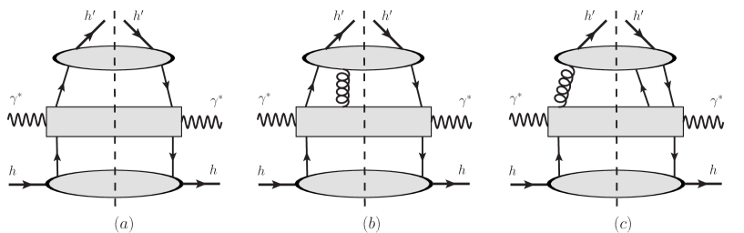
Figure 1: Patterns of diagrams for chiral-odd contributions to $W^{\mu\nu}$. The broken lines are the cuts.

3. One-Loop Chirality-Odd Correction

In this section we study one-loop chiral-odd corrections. They are from those diagrams which have the general patterns given in Fig.1. In Fig.1. the bubbles in the lower part of diagrams represent the parton correlation given by the transversity distribution as in Eq.(4). In Fig.1a the upper bubbles denote two parton correlations of fragmentation, while in Fig.1b and 1c they stand for corresponding three-parton correlations. The boxes in the middle of Fig.1 represent various parton scatterings. Contributions from complex conjugated diagrams of Fig.1b and Fig.1c should also be included. In our case, we only need to consider the real corrections. Hence, there is always one parton crossing the cut in the middle boxes. The virtual corrections are obtained as mentioned before.

In Fig.1 we can in the first step make the projection for the lower bubbles with $h_{1}(x)$ as given in Eq.(4). The projection can be done in a frame in which the initial hadron moves in the $z$-direction, while the final hadron moves in an arbitrary direction. After the projection the contributions from Fig.1a and Fig.1b are:

$$W^{\mu\nu}\biggr{|}_{1a} = \frac{1}{2N_{c}}\int\frac{dx}{x}h_{1}(x)\int d^{4}k_{b}{\rm Tr}\biggr{\{}\gamma\cdot s_{\perp}\gamma\cdot k_{a}{\mathcal{M}}_{1a}^{\mu\nu}(k_{a},k_{b})\Gamma_{1a}(k_{b})\biggr{\}},$$

$$W^{\mu\nu}\biggr{|}_{1b} = \frac{1}{2N_{c}}\int\frac{dx}{x}h_{1}(x)\int d^{4}k_{b}d^{4}k_{g}{\rm Tr}\biggr{\{}\gamma\cdot s_{\perp}\gamma\cdot k_{a}{\mathcal{M}}^{a,\mu\nu\alpha}_{1b}(k_{a},k_{b},k_{g})\Gamma_{1b}^{a,\beta}(k_{b},k_{g})\biggr{\}}g_{\alpha\beta},$$ (26)

with $\Gamma_{1a,1b}$ for the upper bubbles given as:

$$\Gamma_{1a,ij}(k_{b}) = \int\frac{d^{4}\xi}{(2\pi)^{4}}e^{-i\xi\cdot k_{b}}\sum_{X}\langle 0|\psi_{j}(0)|P_{h},X\rangle\langle P_{h},X|\bar{\psi}_{i}(\xi)|0\rangle,$$

$$\Gamma_{1b,ij}^{a,\beta}(k_{b},k_{g}) = \int\frac{d^{4}\xi d^{4}\xi_{1}}{(2\pi)^{4}(2\pi)^{4}}e^{-i\xi\cdot k_{b}-ik_{g}\cdot\xi_{1}}\sum_{X}\langle 0|\psi_{j}(0)|P_{h},X\rangle\langle P_{h},X|\bar{\psi}_{i}(\xi)G^{a,\beta}(\xi_{1})|0\rangle,$$ (27)

where $ij$ stand for Dirac- and color indices. ${\mathcal{M}}_{1a}^{\mu\nu}$ and ${\mathcal{M}}_{1b}^{\mu\nu\alpha}$ stand for the boxes in the middle of Fig.1a and Fig.1b, respectively. The contribution from Fig.1c takes a similar form. $k_{a}$ is the momentum of the quark from the lower bubbles and it is given by $k_{a}=xP$. It is noted that the projection, as given by the $(\cdots)$ in Eq.(4), can be written in a covariant form. After the projections from the lower bubbles we can do projections from the upper bubbles in a frame in which the final hadron moves in the $-z$-direction.

To find the contributions involving twist-3 parts of the upper bubbles one needs to perform collinear expansion for the parts represented by the middle boxes. The expansion includes the expansion of momenta carried by the parton lines connecting the boxes with the bubbles and projecting out perturbative parts from the middle boxes with the different parts of upper bubbles. It is noted that there are contributions at leading twist from Fig.1a. In general it is nontrivial to find the contributions at the next-to-leading twist if there are loops in the middle box. At twist-3 one of the two quark lines entering the upper bubble represents the bad component of the quark field. This component should be eliminated with equation of motion(See [38] and references therein). Since we deal here in fact only with tree-level diagrams with a parton crossing the cut before its momentum is integrated over, the separation is rather easy. One can simply use the twist-3 part in the two-parton correlation in Eq.(9) for the upper bubble in Fig.1a. The diagrams represented by the middle box in Fig.1a at the considered order of $\alpha_{s}$ are given in Fig.2. It is well-known that the existence of the transverse-spin part requires the existence of final state interactions in SIDIS, or nonzero absorptive part in scattering amplitudes. In the contributions of Fig.1a at the order of $\alpha_{s}$, the middle box can not have an absorptive part. The final state interactions can only appear in fragmentation.

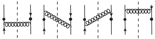
Figure 2: Diagrams for chiral-odd contributions, represented by the middle box in Fig.1a. Black dots denote the insertion of the operator of electromagnetic current.

The contributions from Fig.1b and Fig.1c are of twist-3 or higher twist. Because FF’s from three-parton correlations have the support given in Eq.(11) and are zero if any parton carries zero momentum fraction, one finds at the order of $\alpha_{s}$ that the amplitudes of parton scatterings, represented by the left- or right parts of middle boxes, have no imaginary part, i.e., no physical cut. This is in contrast to chiral-even contributions studied in the next section. Therefore, the needed final state interactions only appear in FF’s. The diagrams represented by the middle box in Fig.1b and Fig.1c are then given by Fig.3 and Fig.4, respectively.

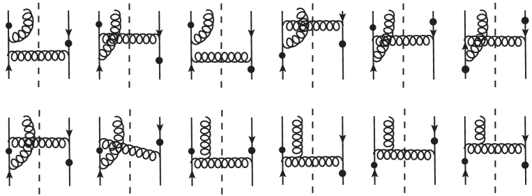
Figure 3: Diagrams for chiral-odd contributions, represented by the middle box in Fig.1b.

Figure 4: Diagrams for chiral-odd contributions, represented by the middle box in Fig.1c.

The calculation is rather straightforward. One needs to perform the collinear expansion in the frame where the final hadron moves in the $-z$-direction. One essentially expands parton momenta $k_{b}$ and $k_{g}$ around the direction of $P_{h}^{\mu}$ and takes the large components of quark fields in the upper bubble of Fig.1b. Details about the expansion can be found in [2, 3]. We first calculate $W^{\mu\nu}$ from Fig.1 with diagrams given explicitly in Fig.2, Fig.3 and Fig.4. The $U(1)$ gauge invariance is checked. From Fig.1a we obtain contributions involving $\hat{e}_{\partial}$ and $\hat{e}_{I}$. We use the relation in Eq.(12) to express $\hat{e}_{I}$ with $\hat{e}_{\partial}$ and $\hat{E}_{F}$. With the obtained $W^{\mu\nu}$ we can calculate our spin-observables. Since there is only one parton in the intermediate state, the length of $P_{h\perp}$ is fixed as:

$$P_{h\perp}\cdot P_{h\perp}=-\frac{zz_{h}Q^{2}}{\hat{x}}(1-\hat{x})(1-\hat{z}).$$ (28)

Therefore, the integration over $P_{h\perp}$ in Eq.(19) can be performed easily. We have then the chiral-odd real corrections:

$$\frac{d\sigma\langle{\mathcal{O}}_{1}\rangle}{dx_{B}dydz_{h}}\biggr{|}_{Re.} = \frac{z_{h}\alpha_{s}\alpha^{2}y}{4Q^{2}}|s_{\perp}|^{2}F_{D}\int\frac{dxdz}{xz}h_{1}(x)\biggr{\{}\hat{e}_{\partial}(z)\biggr{(}-8Y_{M}C_{F}\frac{2}{\epsilon}\delta(1-\hat{x})\delta(1-\hat{z})+{\mathcal{A}}_{1\sigma\partial}(\hat{x},\hat{z})\biggr{)}$$

$$+2\int\frac{dz_{1}}{z_{1}}\biggr{[}{\rm Im}\hat{E}_{F}(z_{1},z){\mathcal{A}}_{1\sigma F}(\hat{x},\hat{z},\hat{z}_{1})+{\rm Im}\hat{E}_{G}(z_{1},z){\mathcal{A}}_{1\sigma G}(\hat{x},\hat{z},\hat{z}_{1})\biggr{]}\biggr{\}},$$

$$\frac{d\sigma\langle{\mathcal{O}}_{2}\rangle}{dx_{B}dydz_{h}}\biggr{|}_{Re.} = \frac{z_{h}\alpha_{s}\alpha^{2}y}{4}|s_{\perp}|^{2}F_{D}Y_{2}\int\frac{dxdz}{xz}h_{1}(x)\biggr{\{}-\hat{e}_{\partial}(z)\frac{8}{\hat{z}}C_{F}\biggr{[}\biggr{(}-2\biggr{(}\frac{2}{\epsilon}\biggr{)}^{2}+3\frac{2}{\epsilon}\biggr{)}\delta(1-\hat{x})\delta(1-\hat{z})$$ (29)

$$+\delta(1-\hat{x})\frac{2}{\epsilon}\frac{2\hat{z}}{(1-\hat{z})_{+}}+\delta(1-\hat{z})\frac{2}{\epsilon}\frac{2\hat{x}}{(1-\hat{x})_{+}}\biggr{]}+\hat{e}_{\partial}(z){\mathcal{A}}_{2\sigma\partial}(\hat{x},\hat{z})+2\int\frac{dz_{1}}{z_{1}}\biggr{[}{\rm Im}\hat{E}_{F}(z_{1},z)$$

$$\biggr{(}\frac{2}{\epsilon}\delta(1-\hat{x})\hat{z}\biggr{(}C_{F}(\hat{z}-\hat{z}_{1}-1)-\frac{N_{c}}{2}\frac{\hat{z}^{2}+\hat{z}_{1}^{2}-\hat{z}-\hat{z}_{1}}{(\hat{z}-\hat{z}_{1})(1-\hat{z}_{1})}\biggr{)}\frac{4}{\hat{z}-\hat{z}_{1}}+{\mathcal{A}}_{2\sigma F}(\hat{x},\hat{z},\hat{z}_{1})\biggr{)}$$

$$+{\rm Im}\hat{E}_{G}(z_{1},z)\biggr{(}\delta(1-\hat{x})\frac{2}{\epsilon}\frac{4C_{F}(\hat{z}-1)^{2}}{N_{c}(1+\hat{z}_{1}-\hat{z})}+{\mathcal{A}}_{2\sigma G}(\hat{x},\hat{z},\hat{z}_{1})\biggr{)}\biggr{]}\biggr{\}},$$

where the poles of $1/\epsilon$ stand for collinear- or I.R. divergences. These divergences come from the momentum region where the unobserved parton in the intermediate state is soft or collinear to the initial- of final hadron. These divergences will be cancelled by those in the virtual parts or subtracted into parton distributions or FF’s as we will show. The integrating ranges of $x$, $z$ and $z_{1}$ are given by:

$$\int dx=\int_{x_{B}}^{1}dx,\quad\int dz=\int_{z_{h}}^{1}dz,\quad\int dz_{1}=\int_{z}^{\infty}dz_{1}.$$ (30)

In Eq.(29) we have already neglected those terms which are proportional to $\epsilon$ and will not contribute to our final results. $F_{D}$ and $\hat{z}_{1}$ are given by:

$$F_{D}=\left(\frac{4\pi\mu_{c}^{2}}{Q^{2}}\right)^{\epsilon/2}\frac{1}{\Gamma(1-\epsilon/2)},\quad\hat{z}_{1}=\frac{z_{h}}{z_{1}}$$ (31)

with $\mu_{c}$ as the scale associated with collinear divergences. In Eq.(29) we have listed divergent contributions explicitly. The finite parts are given by functions ${\mathcal{A}}^{\prime}s$ which can be found in Appendix.

As discussed before, the virtual correction to the derivative part of the hadronic tensor, hence to our observables, is given by the correction of the quark form factor. The correction is well-known. The virtual part can be simply obtained by multiplying our tree-level results in Eq.(24) with the factor:

$$1+\frac{\alpha_{s}C_{F}}{2\pi}F_{D}\biggr{[}-2\left(\frac{2}{\epsilon}\right)^{2}-3\left(\frac{2}{\epsilon}\right)-8\biggr{]}+{\mathcal{O}}(\alpha_{s}^{2}).$$ (32)

Summing the divergent part in the real- and virtual part, we have the divergent parts of one-loop chirality-odd corrections:

$$\frac{d\sigma\langle{\mathcal{O}}_{1}\rangle}{dx_{B}dydz_{h}}\biggr{|}_{Div.} = 0,$$

$$\frac{d\sigma\langle{\mathcal{O}}_{2}\rangle}{dx_{B}dydz_{h}}\biggr{|}_{Div.} = z_{h}\alpha_{s}\alpha^{2}y|s_{\perp}|^{2}Y_{2}F_{D}\left(\frac{2}{\epsilon}\right)\int\frac{dxdz}{xz}h_{1}(x)\biggr{\{}2\hat{e}_{\partial}(z)C_{F}\biggr{(}-3\delta(1-\hat{x})\delta(1-\hat{z})$$ (33)

$$-\frac{2\delta(1-\hat{x})}{(1-\hat{z})_{+}}-\frac{2\hat{x}\delta(1-\hat{z})}{(1-\hat{x})_{+}}\biggr{)}+\delta(1-\hat{x})\int\frac{dz_{1}}{z_{1}}\biggr{[}{\rm Im}\hat{E}_{F}(z_{1},z)\frac{2\hat{z}}{\hat{z}-\hat{z}_{1}}$$

$$\biggr{(}C_{F}(\hat{z}-\hat{z}_{1}-1)-\frac{N_{c}}{2}\frac{\hat{z}^{2}+\hat{z}_{1}^{2}-\hat{z}-\hat{z}_{1}}{(\hat{z}-\hat{z}_{1})(1-\hat{z}_{1})}\biggr{)}+{\rm Im}\hat{E}_{G}(z_{1},z)\frac{2C_{F}(\hat{z}-1)^{2}}{N_{c}(1+\hat{z}_{1}-\hat{z})}\biggr{]}\biggr{\}}.$$

In the sums, the infrared divergences are cancelled. The remaining divergences are collinear ones. The one-loop correction to our first spin observables is finite. The correction to the second observable contains collinear divergences.

It should be noted that the contributions from exchanging collinear partons are in fact already included in the parton distributions and FF’s of the tree-level results in Eq.(24), or they are already contained in the lower- and upper bubbles in Fig.5. In order to avoid double counting, we should subtract these contributions from the one-loop corrections calculated in the above. The subtraction at one-loop level can be easily done with the replacement in the tree-level results in Eq.(24):

$$h_{1}(x)\rightarrow h_{1}(x)-\Delta h_{1}(x),\quad\hat{e}_{\partial}(x)\rightarrow\hat{e}_{\partial}(x)-\Delta\hat{e}_{\partial}(x)$$ (34)

and the contributions which need to be subtracted are:

$$\Delta\frac{d\sigma\langle{\mathcal{O}}_{1}\rangle}{dx_{B}dydz_{h}} = \frac{\pi z_{h}y\alpha^{2}}{Q^{2}}Y_{M}|s_{\perp}|^{2}\epsilon\biggr{(}\Delta h_{1}(x_{B})\hat{e}_{\partial}(z_{h})+h_{1}(x_{B})\Delta\hat{e}_{\partial}(z_{h})\biggr{)},$$

$$\Delta\frac{d\sigma\langle{\mathcal{O}}_{2}\rangle}{dx_{B}dydz_{h}} = -\pi z_{h}y\alpha^{2}Y_{2}|s_{\perp}|^{2}\biggr{(}4-3\epsilon\biggr{)}\biggr{(}\Delta h_{1}(x_{B})\hat{e}_{\partial}(z_{h})+h_{1}(x_{B})\Delta\hat{e}_{\partial}(z_{h})\biggr{)}.$$ (35)

These contributions should be added in our final results to avoid the double counting.

In the case with dimensional regularization for collinear divergences of massless partons, the quantities $\Delta h_{1}$ and $\Delta e_{\partial}$ are determined by the evolution of $h_{1}$ and $\hat{e}_{\partial}$, respectively. The evolution of twist-3 FF’s have been studied in [38, 39, 40]. The evolution of $h_{1}$ can be found in [41]. The evolution of $\hat{e}_{\partial}$ can be found in [38, 40]. According to these results $\Delta h_{1}$ and $\Delta e_{\partial}$ are given by:

$$\Delta h_{1}(x_{B}) = \frac{\alpha_{s}}{2\pi}\biggr{(}-\frac{2}{\epsilon}+\ln\frac{e^{\gamma}\mu^{2}}{4\pi\mu_{c}^{2}}\biggr{)}\int\frac{dx}{x}C_{F}\biggr{(}\frac{2\hat{x}}{(1-\hat{x})_{+}}+\frac{3}{2}\delta(1-\hat{x})\biggr{)}h_{1}(x)$$

$$= \frac{\alpha_{s}}{2\pi}\biggr{(}-\frac{2}{\epsilon}+\ln\frac{e^{\gamma}\mu^{2}}{4\pi\mu_{c}^{2}}\biggr{)}\biggr{(}P_{\perp q}\otimes h_{1}\biggr{)}(x_{B}),$$

$$\Delta\hat{e}_{\partial}(z_{h}) = \frac{\alpha_{s}}{2\pi}\biggr{(}-\frac{2}{\epsilon}+\ln\frac{e^{\gamma}\mu^{2}}{4\pi\mu_{c}^{2}}\biggr{)}\int\frac{dz}{z}\biggr{\{}\hat{e}_{\partial}(z)C_{F}\biggr{(}\frac{2}{(1-\hat{z})_{+}}+\frac{3}{2}\delta(1-\hat{z})\biggr{)}-\int\frac{dz_{1}}{z_{1}}\biggr{[}{\rm Im}\hat{E}_{F}(z_{1},z)$$ (36)

$$\frac{\hat{z}}{\hat{z}-\hat{z}_{1}}\biggr{(}C_{F}(\hat{z}-\hat{z}_{1}-1)-\frac{N_{c}}{2}\frac{\hat{z}^{2}+\hat{z}_{1}^{2}-\hat{z}-\hat{z}_{1}}{(\hat{z}-\hat{z}_{1})(1-\hat{z}_{1})}\biggr{)}+{\rm Im}\hat{E}_{G}(z_{1},z)\frac{C_{F}(\hat{z}-1)^{2}}{N_{c}(1+\hat{z}_{1}-\hat{z})}\biggr{]}\biggr{\}}$$

$$= \frac{\alpha_{s}}{2\pi}\biggr{(}-\frac{2}{\epsilon}+\ln\frac{e^{\gamma}\mu^{2}}{4\pi\mu_{c}^{2}}\biggr{)}\biggr{(}{\mathcal{F}}_{\partial}\otimes\hat{e}_{\partial}+{\mathcal{F}}_{F}\otimes\hat{E}_{F}+{\mathcal{F}}_{G}\otimes\hat{E}_{G}\biggr{)}(z_{h}),$$

where the poles in $\epsilon$ stand for collinear divergence and $\mu$ is the renormalization scale. In Eq.(36) we have introduced four evolution kernels $P_{\perp q}$, ${\mathcal{F}}_{\partial}$ , ${\mathcal{F}}_{F}$ and ${\mathcal{F}}_{G}$ for a short notation. Taking the derivative of $\Delta h_{1}$ and $\Delta e_{\partial}$ with respect to $\ln\mu$ one obtains the evolution of $h_{1}$ and $\hat{e}_{\partial}$, respectively.

Substituting the results in Eq.(36) into the contributions in Eq.(35) and adding them to the divergent part of the one-loop corrections in Eq.(33), one can realize that the divergences represented by the poles in $\epsilon$ are cancelled. The final results of chirality-odd contributions are finite. We will present the final results in Sect. 5.

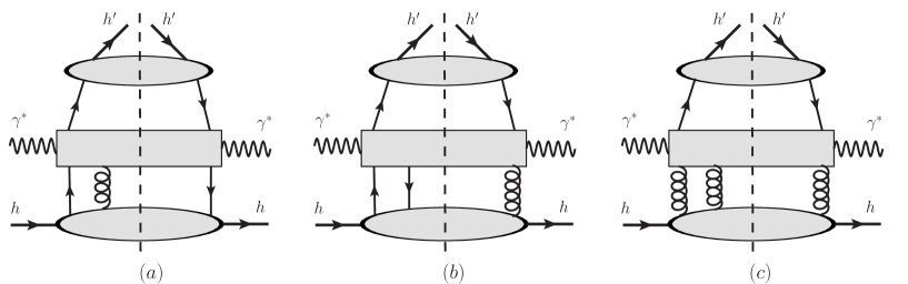
Figure 5: Patterns of diagrams for chiral-even contributions to $W^{\mu\nu}$. The broken lines are the cuts.

4. One-Loop Chirality-Even Correction

In this section we study the one-loop chirality-even corrections. As discussed before, we only need to calculate the real correction. The virtual correction is given by the one-loop correction of the quark form factor. The chirality-even contributions involve twist-2 parton FF’s and twist-3 parton distributions of the initial hadron.

In the case of quark fragmentation, the contributions are from these diagrams, whose general structure can be represented by Fig.5. To calculate, e.g., the contribution from Fig.5a, one can in the first step project out the contribution of the twist-2 quark FF from the upper bubble. After the projection the contribution to $W^{\mu\nu}$ can be written as:

$$W^{\mu\nu}\biggr{|}_{5a}=\int\frac{dz}{z^{d-3}}\hat{d}(z)\int d^{d}k_{a}d^{d}k_{g}{\rm Tr}\biggr{\{}\gamma\cdot P_{h}{\mathcal{M}}_{5a}^{a,\mu\nu\alpha}(k_{a},k_{g},k_{b})\Gamma_{5a}^{a,\beta}(k_{a},k_{g})\biggr{\}}g_{\alpha\beta},$$ (37)

with $\Gamma_{5a}$ for the lower bubble in Fig.5a given as:

$$\Gamma_{5a,ij}^{a,\beta}(k_{a},k_{g})=\int\frac{d^{d}\xi_{a}d^{d}\xi_{g}}{(2\pi)^{2d}}e^{i\xi_{a}\cdot k_{a}+i\xi_{g}\cdot k_{g}}\langle P,s_{\perp}|\bar{\psi}_{j}(0)G^{a,\beta}(\xi_{g})\psi_{i}(\xi_{a})|P,s_{\perp}\rangle$$ (38)

and ${\mathcal{M}}_{5a}^{a,\mu}$ standing for the middle box in Fig.5a. In the above contribution the collinear expansion relevant to the produced hadron is performed and the momentum carried by the quark lines between the middle box and the upper bubble is given by $k_{b}=P_{h}/z$. $k_{a}$ and $k_{g}$ are the momenta carried by the quark- and gluon lines in the low-left part of Fig.5a, respectively.

At the order we consider, there is always one parton contained in the middle boxes crossing the cut. Unlike the case of chiral-odd contributions studied before, where the final-state interactions only appear in parton fragmentation, the final-state interactions in chirality-even contributions can only appear in the middle boxes, i.e., in the hard scatterings. This is due to that twist-2 parton FF’s do not contain final-state interactions. The amplitudes represented by the left parts of the middle boxes have nonzero absorptive part, or the left parts contain a physical cut implicitly. Because of the cut, one of the parton lines in the low-left part of diagrams in Fig.5 can carry zero momentum. The resulted contributions are called as soft-quark- or soft-gluon pole contributions. There are contributions in which none of the parton lines carry zero momentum. These contributions are called as hard-pole contributions. There is also the case that the final hadron is produced through gluon fragmentation. In this case, there are types of diagrams similar to Fig.5.

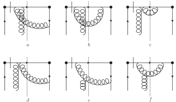
Figure 6: Feynman diagrams for the hard-pole contribution with quark- or gluon fragmentation.

It has been studied in detail how to make the collinear expansion in a gauge-invariant way in [4] and how to calculate the soft-gluon-pole contributions with the master formulas found in [29, 30, 31]. Employing these technics various contributions can be calculated in a straightforward way. Therefore, we will not give the detail of how these calculations are done. We first discuss the contributions of hard-poles. For the case of quark fragmentation, the hard scattering part represented by the middle box in Fig.5a is given by the diagrams in Fig.6, where the quark propagators with a short bar implies the cut for the absorptive part, i.e., only the absorptive part of the propagators is taken into account. The dispersive part will not contribute. Fig.6 stands for two cases, the final hadron can be produced from quark- or gluon fragmentation. The contributions from Fig.6 are:

$$\frac{d\sigma\langle{\mathcal{O}}_{1}\rangle}{dx_{B}dydz_{h}}\biggr{|}_{Fig.6} = \frac{z_{h}y\alpha^{2}\alpha_{s}}{4Q^{2}}|s_{\perp}|^{2}F_{D}\int\frac{dxdz}{xz}\biggr{\{}\hat{d}(z)\biggr{[}Y_{M}T_{F}(x,x_{B})\biggr{(}2N_{c}\left(\frac{2}{\epsilon}\right)^{2}\delta(1-\hat{x})\delta(1-\hat{z})$$

$$-\frac{1+\hat{z}(N_{c}^{2}-1)}{\hat{z}N_{c}}\frac{2}{\epsilon}\delta(1-\hat{x})\frac{1+\hat{z}^{2}}{(1-\hat{z})_{+}}-N_{c}\delta(1-\hat{z})\frac{2}{\epsilon}\frac{1+\hat{x}}{(1-\hat{x})_{+}}\biggr{)}$$

$$+Y_{M}T_{\Delta}(x,x_{B})N_{c}\delta(1-\hat{z})\frac{2}{\epsilon}+T_{F}(x,x_{B}){\mathcal{A}}_{1hq}(\hat{x},\hat{z})+T_{\Delta}(x,x_{B}){\mathcal{B}}_{1hq}(\hat{x},\hat{z})\biggr{]}$$

$$+\hat{g}(z)\biggr{[}Y_{M}T_{F}(x,x_{B})\frac{\hat{z}+N_{c}^{2}(1-\hat{z})}{\hat{z}^{2}N_{c}}\delta(1-\hat{x})\frac{2}{\epsilon}(2-2\hat{z}+z^{2})$$

$$+T_{F}(x,x_{B}){\mathcal{A}}_{1hg}(\hat{x},\hat{z})+T_{\Delta}(x,x_{B}){\mathcal{B}}_{1hg}(\hat{x},\hat{z})\biggr{]}\biggr{\}},$$

$$\frac{d\sigma\langle{\mathcal{O}}_{2}\rangle}{dx_{B}dydz_{h}}\biggr{|}_{Fig.6} = 0.$$ (39)

Here we only list the divergent results explicitly. ${\mathcal{A}}_{1hi}(\hat{x},\hat{z})$ and ${\mathcal{B}}_{1hi}(\hat{x},\hat{z})$ for $i=q,g$ are finite functions given in Appendix. In the following, we will give various contributions in the same way as Eq.(39). From Fig.6 our second observable receives no contributions.

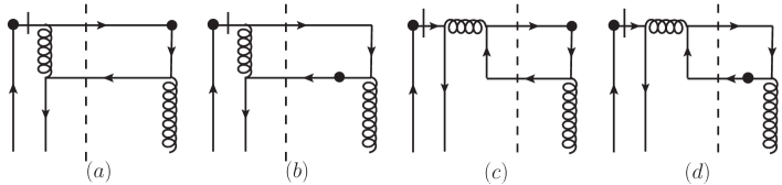
Figure 7: Feynman diagrams for the hard scattering represented by the middle part of Fig.5b. Their contributions are of hard-pole with quark- or antiquark fragmentation.

There are partonic processes as the forward scattering in which a $q\bar{q}$ pair participates as indicated by Fig.5b. Their contributions are given by Fig.7. These contributions are of hard-pole. The contributions from Fig.7 are:

$$\frac{d\sigma\langle{\mathcal{O}}_{1}\rangle}{dx_{B}dydz_{h}}\biggr{|}_{Fig.7} = \frac{z_{h}y\alpha^{2}\alpha_{s}}{4Q^{2}}|s_{\perp}|^{2}F_{D}\int\frac{dxdz}{xz}\biggr{\{}\hat{d}(z)\biggr{[}-\frac{1}{N_{c}}Y_{M}T_{F}(x_{B}-x,x_{B})\frac{2}{\epsilon}\delta(1-\hat{z})(1-2\hat{x})$$

$$+\frac{1}{N_{c}}Y_{M}T_{\Delta}(x_{B}-x,x_{B})\frac{2}{\epsilon}\delta(1-\hat{z})\biggr{]}+T_{F}(x_{B}-x,x_{B})\biggr{(}\hat{d}(z){\mathcal{C}}_{1Fq}(\hat{x},\hat{z})$$

$$-\hat{d}(-z){\mathcal{C}}_{1F\bar{q}}(\hat{x},\hat{z})\biggr{)}+T_{\Delta}(x_{B}-x,x_{B})\biggr{(}\hat{d}(z){\mathcal{C}}_{1Dq}(\hat{x},\hat{z})-\hat{d}(-z){\mathcal{C}}_{1D\bar{q}}(\hat{x},\hat{z})\biggr{)}\biggr{\}},$$

$$\frac{d\sigma\langle{\mathcal{O}}_{2}\rangle}{dx_{B}dydz_{h}}\biggr{|}_{Fig.7} = \frac{z_{h}y\alpha^{2}\alpha_{s}}{4}|s_{\perp}|^{2}Y_{2}\int\frac{dxdz}{xz}\biggr{\{}T_{F}(x_{B}-x,x_{B})\biggr{(}\hat{d}(z){\mathcal{C}}_{2Fq}(\hat{x},\hat{z})$$ (40)

$$-\hat{d}(-z){\mathcal{C}}_{2F\bar{q}}(\hat{x},\hat{z})\biggr{)}+T_{\Delta}(x_{B}-x,x_{B})\biggr{(}\hat{d}(z){\mathcal{C}}_{2Dq}(\hat{x},\hat{z})-\hat{d}(-z){\mathcal{C}}_{1D\bar{q}}(\hat{x},\hat{z})\biggr{)}\biggr{\}}.$$

In the above contributions, one of variables of twist-3 parton distributions $T_{F,\Delta}(x_{1},x_{2})$ is negative, its absolute value is the momentum fraction of the anti-quark. The anti-quark FF is given by $-\hat{d}(-z)$. The contributions from Fig.7 to our second observable is nonzero but finite.

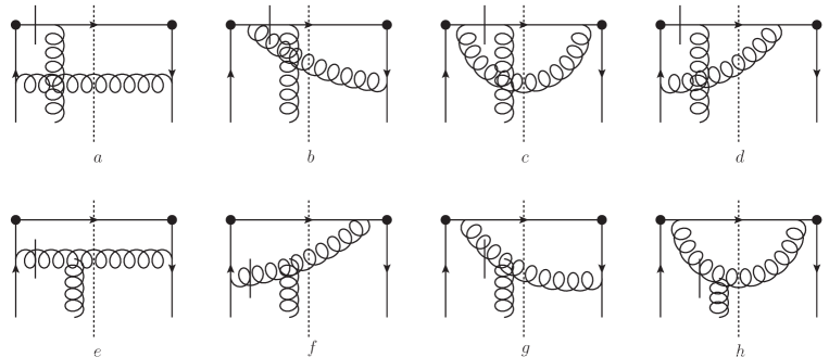
Figure 8: Feynman diagrams for the hard scattering represented by the middle part of Fig.5a. Their contributions are of soft-gluon-pole. Diagrams in the first(second) row are of quark(gluon) fragmentation.

There are soft-pole contributions, in which one of initial partons carries zero momentum. This parton can be a gluon or quark. The soft-gluon pole contributions can be calculated conveniently with the master formulas found in [29, 30, 31]. From the type of diagrams of Fig.5a there are soft-gluon-pole contributions. They are given by diagrams in Fig.8. In Fig.8 the diagrams of the first row are for quark fragmentation, those in the second row are for gluon fragmentation. The total contributions from Fig.8 are:

$$\frac{d\sigma\langle{\mathcal{O}}_{1}\rangle}{dx_{B}dydz_{h}}\biggr{|}_{Fig.8} = \frac{z_{h}y\alpha^{2}\alpha_{s}}{4Q^{2}}|s_{\perp}|^{2}F_{D}\int\frac{dxdz}{xz}T_{F}(x,x)\biggr{\{}\hat{d}(z)\biggr{[}\frac{1}{\hat{z}N_{c}}Y_{M}\biggr{(}(\epsilon-2)\left(\frac{2}{\epsilon}\right)^{2}\delta(1-\hat{x})\delta(1-\hat{z})$$

$$+\frac{2}{\epsilon}\frac{1+\hat{z}^{2}}{(1-\hat{z})_{+}}\delta(1-\hat{x})+\frac{2}{\epsilon}\frac{1+\hat{x}^{2}}{(1-\hat{x})_{+}}\delta(1-\hat{z})\biggr{)}+{\mathcal{D}}_{1q}(\hat{x},\hat{z})\biggr{]}$$

$$+\hat{g}(z)\biggr{[}\frac{N_{c}}{\hat{z}^{2}}Y_{M}\biggr{(}-\frac{2}{\epsilon}\delta(1-\hat{x})(2-2\hat{z}+\hat{z}^{2})\biggr{)}+{\mathcal{D}}_{1g}(\hat{x},\hat{z})\biggr{]}\biggr{\}},$$

$$\frac{d\sigma\langle{\mathcal{O}}_{2}\rangle}{dx_{B}dydz_{h}}\biggr{|}_{Fig.8} = 0.$$ (41)

Our second observable does not receive contributions from Fig.8.

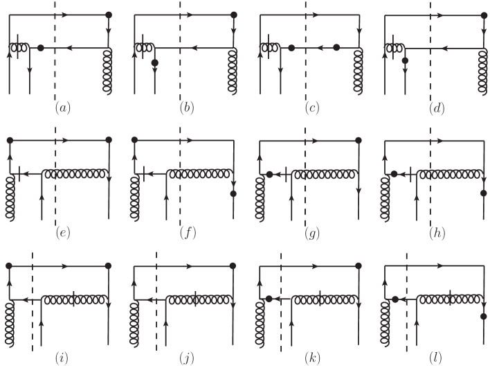
Figure 9: Feynman diagrams for the hard scattering represented by the middle part of Fig.5b. Their contributions are of soft-quark-pole.

From the type of diagrams of Fig.5b there are soft-quark-pole contributions. The diagrams are given in Fig.9. There are contributions involving quark-, antiquark and gluon fragmentation functions. The contributions from gluon fragmentation are represented by the diagrams in the second row. Those from antiquark fragmentation are given by the first- and third row. Contributions with quark fragmentation are from all three rows of Fig.9. But the contributions from the second row cancel those from the complex conjugated diagrams of third row. This is because the diagrams in the third row are from the second row by cutting the unobserved parton lines in different ways. It is easy to show the cancellation. Therefore, the contributions of quark fragmentation are only from the first row. We have:

$$\frac{d\sigma\langle{\mathcal{O}}_{1}\rangle}{dx_{B}dydz_{h}}\biggr{|}_{Fig.9} = \frac{z_{h}y\alpha^{2}\alpha_{s}}{4Q^{2}}|s_{\perp}|^{2}\int\frac{dxdz}{xz}\biggr{\{}\hat{d}(z)\biggr{[}T_{F}(-x,0){\mathcal{E}}_{1Fq}(\hat{x},\hat{z})+T_{\Delta}(-x,0){\mathcal{E}}_{1\Delta q}(\hat{x},\hat{z})\biggr{]}$$

$$-\hat{d}(-z)\biggr{[}T_{F}(0,x){\mathcal{E}}_{1F\bar{q}}(\hat{x},\hat{z})+T_{\Delta}(0,x){\mathcal{E}}_{1\Delta\bar{q}}(\hat{x},\hat{z})\biggr{]}$$

$$+\hat{g}(z)\biggr{[}T_{F}(x,0){\mathcal{E}}_{1Fg}(\hat{x},\hat{z})+T_{\Delta}(x,0){\mathcal{E}}_{1\Delta g}(\hat{x},\hat{z})\biggr{]}\biggr{\}},$$

$$\frac{d\sigma\langle{\mathcal{O}}_{2}\rangle}{dx_{B}dydz_{h}}\biggr{|}_{Fig.9} = \frac{z_{h}y\alpha^{2}\alpha_{s}}{4}|s_{\perp}|^{2}Y_{2}\int\frac{dxdz}{xz}\biggr{\{}\hat{d}(z)\biggr{[}T_{F}(-x,0){\mathcal{E}}_{2Fq}(\hat{x},\hat{z})+T_{\Delta}(-x,0){\mathcal{E}}_{2\Delta q}(\hat{x},\hat{z})\biggr{]}$$ (42)

$$-\hat{d}(-z)\biggr{[}T_{F}(0,x){\mathcal{E}}_{2F\bar{q}}(\hat{x},\hat{z})+T_{\Delta}(0,x){\mathcal{E}}_{2\Delta\bar{q}}(\hat{x},\hat{z})\biggr{]}$$

$$+\hat{g}(z)\biggr{[}T_{F}(x,0){\mathcal{E}}_{2Fg}(\hat{x},\hat{z})+T_{\Delta}(x,0){\mathcal{E}}_{2\Delta g}(\hat{x},\hat{z})\biggr{]}\biggr{\}}.$$

The soft-quark-pole contributions are finite.

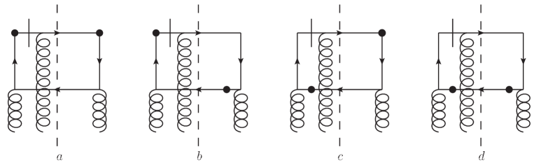
Figure 10: Feynman diagrams for the hard scattering represented by the middle part of Fig.5c. Their contributions are of soft-gluon-pole

At the order we consider, there are contributions involving gluonic twist-3 parton distributions defined in Eq.(7). These contributions are represented by the type of diagrams specified in Fig.5c. Since there are three gluons exchanged between the middle box and the lower bubble, the Bose-symmetry should be kept. For this it is convenient to use the symmetric notation in [31, 32, 42] for the twist-3 gluonic matrix elements in the calculation and to express the final result with the gluonic distributions in Eq.(7). In the symmetric notation the matrix element of twist-3 gluonic operator can be parameterized as:

$$\frac{i^{3}g_{s}}{P^{+}}\int\frac{d\lambda_{1}}{2\pi}\frac{d\lambda_{2}}{2\pi}e^{i\lambda_{1}x_{1}P^{+}+i\lambda_{2}(x_{2}-x_{1})P^{+}}\langle P,s_{\perp}|G^{a,+\alpha}(\lambda_{1}n)G^{c,+\gamma}(\lambda_{2}n)G^{b,+\beta}(0)|P,s_{\perp}\rangle$$

$$=\frac{N_{c}}{(N_{c}^{2}-1)(N_{c}^{2}-4)}d^{abc}O^{\alpha\beta\gamma}(x_{1},x_{2})-\frac{i}{N_{c}(N_{c}^{2}-1)}f^{abc}N^{\alpha\beta\gamma}(x_{1},x_{2}),$$ (43)

where all indices $\alpha,\beta$ and $\gamma$ are transverse. From Bose-symmetry and covariance the two tensors take the form:

$$O^{\alpha\beta\gamma}(x_{1},x_{2}) = -2i\biggr{[}O(x_{1},x_{2})g^{\alpha\beta}\tilde{s}_{\perp}^{\gamma}+O(x_{2},x_{2}-x_{1})g^{\beta\gamma}\tilde{s}_{\perp}^{\alpha}+O(x_{1},x_{1}-x_{2})g^{\gamma\alpha}\tilde{s}_{\perp}^{\beta}\biggr{]},$$

$$N^{\alpha\beta\gamma}(x_{1},x_{2}) = -2i\biggr{[}N(x_{1},x_{2})g^{\alpha\beta}\tilde{s}_{\perp}^{\gamma}-N(x_{2},x_{2}-x_{1})g^{\beta\gamma}\tilde{s}_{\perp}^{\alpha}-N(x_{1},x_{1}-x_{2})g^{\gamma\alpha}\tilde{s}_{\perp}^{\beta}\biggr{]},$$ (44)

with the properties of the function $O$ and $N$

$$O(x_{1},x_{2})=O(x_{2},x_{1}),\quad O(x_{1},x_{2})=O(-x_{1},-x_{2}),\quad N(x_{1},x_{2})=N(x_{2},x_{1}),$$

$$N(x_{1},x_{2})=-N(-x_{1},-x_{2}).$$ (45)

The function $O$ and $N$ are related to those defined in Eq.(7) as

$$T_{G}^{(f)}(x_{1},x_{2}) = 2\pi\biggr{(}(d-2)N(x_{1},x_{2})-N(x_{2},x_{2}-x_{1})-N(x_{1},x_{1}-x_{2})\biggr{)},$$

$$T_{G}^{(d)}(x_{1},x_{2}) = 2\pi\biggr{(}(d-2)O(x_{1},x_{2})+O(x_{2},x_{2}-x_{1})+O(x_{1},x_{1}-x_{2})\biggr{)}.$$ (46)

It should be noted that the relations depend on $d=4-\epsilon$. It will affect on the subtraction discussed later.

With the symmetric notation, the middle box of Fig.5c is given by diagrams in Fig.10. The contributions from Fig.5c are of soft-gluon-pole, i.e., one of the three gluon-lines carries zero momentum. One can use the so-called master formula in [29, 30, 31] to calculate the twist-3 contributions. From Fig.10 we have:

$$\frac{d\sigma\langle{\mathcal{O}}_{1}\rangle}{dx_{B}dydz_{h}}\biggr{|}_{Fig.10} = \frac{z_{h}y\alpha^{2}\alpha_{s}}{4Q^{2}}|s_{\perp}|^{2}F_{D}(-4\pi)\int\frac{dxdz}{x^{2}z}\hat{d}(z)\biggr{\{}\biggr{(}O(x,x)+N(x,x)+O(x,0)-N(x,0)\biggr{)}$$

$$\biggr{[}Y_{M}\frac{2}{\epsilon}\delta(1-\hat{z})(1-2\hat{x}+2\hat{x}^{2})+Y_{L}{\mathcal{F}}_{1L}(\hat{x},\hat{z})\biggr{]}+Y_{M}\biggr{(}O(x,x)+N(x,x)\biggr{)}$$

$${\mathcal{F}}_{1M+}(\hat{x},\hat{z})+Y_{M}\biggr{(}O(x,0)-N(x,0)\biggr{)}{\mathcal{F}}_{1M-}(\hat{x},\hat{z})\biggr{\}},$$

$$\frac{d\sigma\langle{\mathcal{O}}_{2}\rangle}{dx_{B}dydz_{h}}\biggr{|}_{Fig.10} = \frac{z_{h}y\alpha^{2}\alpha_{s}}{4}|s_{\perp}|^{2}Y_{2}(-4\pi)\int\frac{dxdz}{x^{2}z}\hat{d}(z)\biggr{(}O(x,0)-N(x,0)\biggr{)}\frac{4\hat{x}^{2}}{\hat{z}}.$$ (47)

We observe that the contribution from Fig.10 to our second observable is finite.

The real part of one-loop chirality-even correction to our observables is the sum of the contributions listed in Eq.(39, 40, 41, 42, 47). The virtual part, as mentioned before, is obtained by multiplying our tree-level results in Eq.(24) by the factor in Eq.(32). Since our second observable at tree-level does not contain chirality-even part, its virtual part of the chirality-even part is zero. Adding all divergent contributions together, we obtain the sum:

$$\frac{d\sigma\langle{\mathcal{O}}_{1}\rangle}{dx_{B}dydz_{h}}\biggr{|}_{Div.} = \frac{z_{h}y\alpha^{2}\alpha_{s}}{2Q^{2}}|s_{\perp}|^{2}Y_{M}F_{D}\int\frac{dxdz}{xz}\left(-\frac{2}{\epsilon}\right)\biggr{\{}\delta(1-\hat{x})T_{F}(x,x)\biggr{(}{\mathcal{P}}_{qq}(\hat{z})\hat{d}(z)$$

$$+{\mathcal{P}}_{gq}(\hat{z})\hat{g}(z)\biggr{)}+\delta(1-\hat{z})\hat{d}(z)\biggr{[}\biggr{(}{\mathcal{P}}_{qq}(\hat{x})-\frac{N_{c}}{2}\frac{1+\hat{x}^{2}}{(1-\hat{x})_{+}}-N_{c}\delta(1-\hat{x})\biggr{)}T_{F}(x,x)$$

$$+\frac{N_{c}}{2}\frac{1+\hat{x}}{(1-\hat{x})_{+}}T_{F}(x,x_{B})+\frac{N_{c}}{2}T_{\Delta}(x_{B},x)+\frac{1}{2N_{c}}T_{\Delta}(x_{B},x_{B}-x)$$

$$+\frac{1}{2N_{c}}(1-2\hat{x})T_{F}(x_{B},x_{B}-x)-\frac{1}{2x}(1-2\hat{x}+2\hat{x}^{2})T_{G+}(x,x)\biggr{]}\biggr{\}},$$

$$\frac{d\sigma\langle{\mathcal{O}}_{2}\rangle}{dx_{B}dydz_{h}}\biggr{|}_{Div.} = 0,$$ (48)

with the standard splitting functions:

$${\mathcal{P}}_{qq}(z)=C_{F}\biggr{(}\frac{1+z^{2}}{(1-z)_{+}}+\frac{3}{2}\delta(1-z)\biggr{)},\quad{\mathcal{P}}_{gq}(z)=C_{F}\frac{2-2z+z^{2}}{z}.$$ (49)

In Eq.(48) and in our final results the contributions from gluonic twist-3 distributions can be conveniently expressed by two combinations $T_{G\pm}(x_{1},x_{2})$ of gluonic twist-3 distributions. They are defined as:

$$T_{G\pm}(x_{1},x_{2})=T_{G}^{(f)}(x_{1},x_{2})\pm T_{G}^{(d)}(x_{1},x_{2}).$$ (50)

In Eq.(48) the divergent gluonic contribution is only related to $T_{G+}(x,x)$, which are given by those twist-3 gluonic distributions in Eq.(44) as:

$$T_{G+}(x,x) = 2\pi\biggr{[}2\biggr{(}O(x,x)+N(x,x)+O(x,0)-N(x,0)\biggr{)}-\epsilon\biggr{(}O(x,x)+N(x,x)\biggr{)}\biggr{]}.$$ (51)

Inspecting Eq.(48), we find that our second observable is finite, while the first one is divergent. The divergence is represented by the single pole in $\epsilon$. The divergence of double pole in the real- and virtual part is cancelled in the sum. The divergence in Eq.(48) comes from the exchanged parton in the kinematic region of momentum which is collinear to the initial hadron $h$ or the final $h^{\prime}$. This divergent contribution from the collinear region is in fact already included in the tree-level result of the chiral-even part of our first observable in Eq.(24), i.e., in the twist-3 parton distributions and twist-2 parton FF’s. Therefore, this divergent contribution needs to be subtracted to avoid a double counting.

The subtraction can be done by the replacement in the chirality-even part of the tree-level results in Eq.(24):

$$T_{F}(x,x)\rightarrow T_{F}(x,x)-\Delta T_{F}(x,x),\quad\hat{d}(z)\rightarrow\hat{d}(z)-\Delta\hat{d}(z).$$ (52)

The contributions which should be added in the final results for the subtraction are:

$$\Delta\frac{d\sigma\langle{\mathcal{O}}_{1}\rangle}{dx_{B}dydz_{h}} = -\pi\frac{z_{h}y\alpha^{2}\alpha_{s}}{Q^{2}}|s_{\perp}|^{2}Y_{M}\biggr{(}1-\frac{\epsilon}{2}\biggr{)}\biggr{[}\Delta\hat{d}(z_{h})T_{F}(x_{B},x_{B})+\hat{d}(z_{h})\Delta T_{F}(x_{B},x_{B})\biggr{]},$$

$$\Delta\frac{d\sigma\langle{\mathcal{O}}_{2}\rangle}{dx_{B}dydz_{h}} = 0.$$ (53)

In dimensional regularization for regularizing all divergences, the quantities $\Delta\hat{d}(z)$ and $\Delta T_{F}(x,x)$ are determined by the evolution kernels. The evolution kernel of the quark fragmentation function is well-known. The evolution of $T_{F}(x,x)$ is studied in [43, 44, 45, 46, 47, 48]. At one-loop level we have:

$$\Delta T_{F}(x,x) = \frac{\alpha_{s}}{2\pi}\left(-\frac{2}{\epsilon_{c}}+\ln\frac{e^{\gamma}\mu^{2}}{4\pi\mu_{c}^{2}}\right)\biggr{\{}-N_{c}T_{F}(x,x)+\int_{x}^{1}\frac{dz}{z}\biggr{[}{\mathcal{P}}_{qq}(z)T_{F}(\xi,\xi)+\frac{N_{c}}{2}\biggr{(}T_{\Delta}(x,\xi)$$

$$+\frac{(1+z)T_{F}(x,\xi)-(1+z^{2})T_{F}(\xi,\xi)}{1-z}\biggr{)}+\frac{1}{2N_{c}}\biggr{(}(1-2z)T_{F}(x,x-\xi)$$

$$+T_{\Delta}(x,x-\xi)\biggr{)}-\frac{1}{2}\frac{(1-z)^{2}+z^{2}}{\xi}T_{G+}(\xi,\xi)\biggr{]}\biggr{\}}$$

$$= \frac{\alpha_{s}}{2\pi}\left(-\frac{2}{\epsilon_{c}}+\ln\frac{e^{\gamma}\mu^{2}}{4\pi\mu_{c}^{2}}\right)\biggr{(}{\mathcal{F}}_{q}\otimes T_{F}+{\mathcal{F}}_{\Delta q}\otimes T_{\Delta}+{\mathcal{F}}_{g}\otimes T_{G+}\biggr{)}(x),$$

$$\Delta\hat{d}(x) = \frac{\alpha_{s}}{2\pi}\left(-\frac{2}{\epsilon_{c}}+\ln\frac{e^{\gamma}\mu^{2}}{4\pi\mu_{c}^{2}}\right)\int\frac{d\xi}{\xi}\biggr{\{}P_{qq}(z)\hat{d}(\xi)+P_{gq}(z)\hat{g}(\xi)\biggr{\}}$$ (54)

$$= \frac{\alpha_{s}}{2\pi}\left(-\frac{2}{\epsilon_{c}}+\ln\frac{e^{\gamma}\mu^{2}}{4\pi\mu_{c}^{2}}\right)\biggr{(}{\mathcal{P}}_{qq}\otimes\hat{d}+{\mathcal{P}}_{gq}\otimes\hat{g}\biggr{)}(x),$$

with $z=x/\xi$. In the above we define five convolutions ${\mathcal{F}}$’s and ${\mathcal{P}}$’s for short notations. $\mu$ is the renormalization scale. $\mu_{c}$ is the scale related to collinear divergences. The derivative of $\Delta T_{F}(x,x)$ with respect to $\mu$ gives the evolution kernel of $T_{F}(x,x)$ derived. Adding the contributions in Eq.(53) to our calculated one-loop correction, we find that the chirality-even part of the one-loop correction is finite.

The chirality-even corrections to our first observable have been studied in [23, 24, 25]. In [24] the contributions from Fig.10 are obtained, where there is a soft-gluon-pole contributions involving the derivative of $N(x,x)$ or $N(x,0)$ with respect to $x$, and the derivative of $O(x,x)$ or $O(x,0)$. These derivative terms can be eliminated by integration by part. It is noted that there is an integration over $P_{h\perp}$ in Eq.(19) for our spin observables. With the master formulas in [29, 30, 31], such derivative terms are eliminated automatically through the integration over $P_{h\perp}$. This also holds for the case of $T_{F}(x,x)$, where there is a derivative contribution of $T_{F}(x,x)$ in [23]. In [23] the contributions from Fig.6 and Fig.8 are obtained, but without the contributions from $T_{\Delta}(x_{1},x_{2})$. In [25] the contributions with $T_{\Delta}(x_{1},x_{2})$ from Fig.6 and Fig.8 and the contributions from Fig.7 are included. But, the soft-quark-pole contributions are still missing. In all these works, only the first term with $g^{\mu\nu}$ in the first equation in Eq.(22) is taken into account and the contributions from the second term with $Y_{L}$ are not considered. It is true that the second term with $Y_{L}$ does not contribute at tree-level. But it will contribute beyond tree-level. Except these missing contributions our results agree with those in [23, 24, 25]. The missing contributions with $Y_{L}$ and the soft-quark-pole contributions are included in this work, they are finite.

5. Final Results

As mentioned in previous sections, the evolutions of involved parton distributions and FF’s take the forms of convolutions. We denote these evolutions as:

$$\frac{\partial\hat{d}(z)}{\partial\ln\mu} = \frac{\alpha_{s}}{\pi}\biggr{(}{\mathcal{P}}_{qq}\otimes\hat{d}+{\mathcal{P}}_{gq}\otimes\hat{g}\biggr{)}(z),$$

$$\frac{\partial T_{F}(x,x)}{\partial\ln\mu} = \frac{\alpha_{s}}{\pi}\biggr{(}{\mathcal{F}}_{q}\otimes T_{F}+{\mathcal{F}}_{\Delta q}\otimes T_{\Delta}+{\mathcal{F}}_{g}\otimes T_{G+}\biggr{)}(x),$$

$$\frac{\partial h_{1}(x)}{\partial\ln\mu} = \frac{\alpha_{s}}{\pi}\biggr{(}P_{\perp q}\otimes h_{1}\biggr{)}(x),$$

$$\frac{\partial\hat{e}_{\partial}(z)}{\partial\ln\mu} = \frac{\alpha_{s}}{\pi}\biggr{(}{\mathcal{F}}_{\partial}\otimes\hat{e}_{\partial}+{\mathcal{F}}_{F}\otimes\hat{E}_{F}+{\mathcal{F}}_{G}\otimes\hat{E}_{G}\biggr{)}(z).$$ (55)

The definitions of the convolutions can be found in Eq.(36) and Eq.(54). With these notations we can write our final results in the form which are explicitly $\mu$-independent at one-loop level:

$$\frac{d\sigma\langle{\mathcal{O}}_{1}\rangle}{dx_{B}dydz_{h}} = \frac{\pi z_{h}y\alpha^{2}}{Q^{2}}|s_{\perp}|^{2}Y_{M}\biggr{[}\hat{d}(z_{h})T_{F}(x_{B},x_{B})-\frac{1}{2}\ln\frac{e\mu^{2}}{Q^{2}}\frac{\partial}{\partial\ln\mu}\biggr{(}T_{F}(x_{B},x_{B})\hat{d}(z_{h})\biggr{)}$$

$$-\frac{\partial}{\partial\ln\mu}\biggr{(}h_{1}(x_{B})\hat{e}_{\partial}(z_{h})\biggr{)}-\frac{\alpha_{s}}{2\pi}C_{F}\biggr{(}5\hat{d}(z_{h})T_{F}(x_{B},x_{B})-6h_{1}(x_{B})\hat{e}_{\partial}(z_{h})\biggr{)}$$

$$+\frac{\alpha_{s}}{8\pi}\hat{d}(z_{h})\int\frac{dx}{x^{2}}((1-\hat{x})^{2}+\hat{x}^{2})\biggr{(}3T_{G+}(x,x)-2T_{G-}(x,0)\biggr{)}\biggr{]}+\frac{d\sigma\langle{\mathcal{O}}_{1}\rangle_{F}}{dx_{B}dydz_{h}},$$

$$\frac{d\sigma\langle{\mathcal{O}}_{2}\rangle}{dx_{B}dydz_{h}} = 2\pi z_{h}y\alpha^{2}|s_{\perp}|^{2}Y_{2}\biggr{[}2h_{1}(x_{B})\hat{e}_{\partial}(z_{h})-\biggr{(}\ln\frac{\mu^{2}}{Q^{2}}+\frac{3}{2}\biggr{)}\frac{\partial}{\partial\ln\mu}\biggr{(}h_{1}(x_{B})\hat{e}_{\partial}(z_{h})\biggr{)}$$ (56)

$$-\frac{5\alpha_{s}}{2\pi}C_{F}h_{1}(x_{B})\hat{e}_{\partial}(z_{h})\biggr{]}+\frac{d\sigma\langle{\mathcal{O}}_{2}\rangle_{F}}{dx_{B}dydz_{h}},$$

where the last term with the sub-index $F$ in the result of our two observables is the sum of all finite contributions from sets of diagrams studied in previous sections. The sums are:

$$\frac{d\sigma\langle{\mathcal{O}}_{1}\rangle_{F}}{dx_{B}dydz_{h}} = \frac{z_{h}\alpha_{s}\alpha^{2}y}{4Q^{2}}|s_{\perp}|^{2}\int\frac{dxdz}{xz}\biggr{\{}h_{1}(x)\biggr{[}\hat{e}_{\partial}(z){\mathcal{A}}_{1\sigma\partial}(\hat{x},\hat{z})$$

$$+2\int\frac{dz_{1}}{z_{1}}\biggr{(}{\rm Im}\hat{E}_{F}(z_{1},z){\mathcal{A}}_{1\sigma F}(\hat{x},\hat{z},\hat{z}_{1})+{\rm Im}\hat{E}_{G}(z_{1},z){\mathcal{A}}_{1\sigma G}(\hat{x},\hat{z})\biggr{)}\biggr{]}$$

$$+\hat{d}(z)\biggr{[}T_{F}(x,x_{B}){\mathcal{A}}_{1hq}(\hat{x},\hat{z})+T_{\Delta}(x,x_{B}){\mathcal{B}}_{1hq}(\hat{x},\hat{z})+T_{F}(x_{B}-x,x_{B}){\mathcal{C}}_{1Fq}(\hat{x},\hat{z})$$

$$+T_{\Delta}(x_{B}-x,x_{B}){\mathcal{C}}_{1Dq}(\hat{x},\hat{z})+T_{F}(x,x){\mathcal{D}}_{1q}(\hat{x},\hat{z})+T_{F}(-x,0){\mathcal{E}}_{1Fq}(\hat{x},\hat{z})$$

$$+T_{\Delta}(-x,0){\mathcal{E}}_{1\Delta q}(\hat{x},\hat{z})+\frac{1}{x}T_{G+}(x,x){\mathcal{F}}_{1g+}(\hat{x},\hat{z})+\frac{1}{x}T_{G-}(x,0){\mathcal{F}}_{1g-}(\hat{x},\hat{z})\biggr{]}$$

$$-\hat{d}(-z)\biggr{[}T_{F}(x_{B}-x,x_{B}){\mathcal{C}}_{1F\bar{q}}(\hat{x},\hat{z})+T_{\Delta}(x_{B}-x,x_{B}){\mathcal{C}}_{1D\bar{q}}(\hat{x},\hat{z})$$

$$+T_{F}(0,x){\mathcal{E}}_{1F\bar{q}}(\hat{x},\hat{z})+T_{\Delta}(0,x){\mathcal{E}}_{1\Delta\bar{q}}(\hat{x},\hat{z})\biggr{]}$$

$$+\hat{g}(z)\biggr{[}T_{F}(x,x_{B}){\mathcal{A}}_{1hg}(\hat{x},\hat{z})+T_{\Delta}(x,x_{B}){\mathcal{B}}_{1hg}(\hat{x},\hat{z})$$

$$+T_{F}(x,x){\mathcal{D}}_{1g}(\hat{x},\hat{z})+T_{F}(x,0){\mathcal{E}}_{1Fg}(\hat{x},\hat{z})+T_{\Delta}(x,0){\mathcal{E}}_{1\Delta g}(\hat{x},\hat{z})\biggr{]}\biggr{\}},$$

$$\frac{d\sigma\langle{\mathcal{O}}_{2}\rangle_{F}}{dx_{B}dydz_{h}} = \frac{z_{h}\alpha_{s}\alpha^{2}y}{4}|s_{\perp}|^{2}\int\frac{dxdz}{xz}\biggr{\{}h_{1}(x)\biggr{[}\hat{e}_{\partial}(z){\mathcal{A}}_{2\sigma\partial}(\hat{x},\hat{z})$$ (57)

$$+2\int\frac{dz_{1}}{z_{1}}\biggr{(}{\rm Im}\hat{E}_{F}(z_{1},z){\mathcal{A}}_{2\sigma F}(\hat{x},\hat{z},\hat{z}_{1})+{\rm Im}\hat{E}_{G}(z_{1},z){\mathcal{A}}_{2\sigma G}(\hat{x},\hat{z})\biggr{)}\biggr{]}$$

$$+\hat{d}(z)\biggr{[}T_{F}(x_{B}-x,x_{B}){\mathcal{C}}_{2Fq}(\hat{x},\hat{z})+T_{\Delta}(x_{B}-x,x_{B}){\mathcal{C}}_{2Dq}(\hat{x},\hat{z})$$

$$+T_{F}(-x,0){\mathcal{E}}_{2Fq}(\hat{x},\hat{z})+T_{\Delta}(-x,0){\mathcal{E}}_{2\Delta q}(\hat{x},\hat{z})+\frac{2\hat{x}^{2}}{x\hat{z}}(T_{G+}(x,x)+2T_{G-}(x,0))\biggr{]}$$

$$-\hat{d}(-z)\biggr{[}T_{F}(x_{B}-x,x_{B}){\mathcal{C}}_{1F\bar{q}}(\hat{x},\hat{z})+T_{\Delta}(x_{B}-x,x_{B}){\mathcal{C}}_{1D\bar{q}}(\hat{x},\hat{z})$$

$$+T_{F}(0,x){\mathcal{E}}_{1F\bar{q}}(\hat{x},\hat{z})+T_{\Delta}(0,x){\mathcal{E}}_{1\Delta\bar{q}}(\hat{x},\hat{z})\biggr{]}$$

$$+\hat{g}(z)\biggr{[}T_{F}(x,0){\mathcal{E}}_{2Fg}(\hat{x},\hat{z})+T_{\Delta}(x,0){\mathcal{E}}_{2\Delta g}(\hat{x},\hat{z})\biggr{]}\biggr{\}}.$$

Eq.(56,57) are our main results. The perturbative functions ${\mathcal{A}}$’s, ${\mathcal{B}}$’s, ${\mathcal{C}}$’s and ${\mathcal{E}}$’s are given in Appendix. In Eq.(24) and the results in this section the contributions from charge-conjugated parton processes are not included. They can be obtained from our results with charge-conjugation.

6. Summary

In this work we have studied two spin observables of SIDIS in which the initial hadron is transversely polarized. They are weighted differential cross-sections corresponding to Sivers- or Collins asymmetry, respectively. These asymmetries have been measured in experiment already. In fact, one of the studied observables is weighted Sivers asymmetry, while another is weighted Collins asymmetry. In collinear factorization they take factorized forms as convolutions of perturbative coefficient functions with twist-3 parton distributions combined twist-2 FF’s or twist-2 transversity distribution combined with twist-3 FF’s. The perturbative coefficient functions have been calculated at one-loop level in this work. The collinear divergences are correctly subtracted so that these functions are finite. With our results the spin observables or SSA’s are predicted more precisely than with tree-level results. The spin observables studied here can already be measured in current COMPASS- and JLab experiment, and in future experiment at EIC.

It is interesting to note that at tree-level our first observable is predicted only with ETQS matrix element and the twist-2 quark FF, and the second observable is predicted only with the twist-2 transversity distribution and one of twist-3 quark FF’s. This implies that through the measurement of these observables, it is possible to determine these nonperturbative quantities at tree-level accuracy. But, at one-loop level more twist-3 parton distributions and FF’s are involved. To determine all involved parton distributions and FF’s, one has to combine theoretical- and experimental results from other processes, like Drell-Yan processes and inclusive single hadron production at hadron-hadron collisions, where the involved parton distributions and FF’s also appear in theoretical predictions. This requires more studies both in theory and experiment.

Acknowledgments

The work is supported by National Nature Science Foundation of P.R. China(No.11275244, 11675241, 11605195). The partial support from the CAS center for excellence in particle physics(CCEPP) is acknowledged.

Appendix

We list here all functions appearing in the finite part of our results. We define two functions

$$L_{\pm}(\xi)=\left(\frac{\ln(1-\xi)}{1-\xi}\right)_{+}\pm\frac{\ln\xi}{1-\xi}.$$ (A.1)

The functions in the chirality-odd contributions in Eq.(29) are:

$$\mathcal{A}_{1\sigma\partial} = 8Y_{M}C_{F}\biggr{(}\delta(1-\hat{x})\frac{1}{(1-\hat{z})_{+}}+\delta(1-\hat{z})\frac{\hat{x}}{(1-\hat{x})_{+}}\biggr{)},$$ (A.2)

$$\mathcal{A}_{1\sigma F} = \frac{Y_{M}}{\hat{z}(\hat{z}-\hat{z}_{1})^{2}}\biggr{[}2C_{F}\hat{z}_{1}\biggr{(}-3\hat{z}^{2}+\hat{z}(\hat{z}_{1}+4)-2\hat{z}_{1}\biggr{)}-\frac{1}{N_{c}}\hat{z}\biggr{(}\hat{x}(\hat{z}_{1}-\hat{z})+2(\hat{z}-1)\hat{z}_{1}\biggr{)}$$ (A.3)

$$-\delta(1-\hat{x})\frac{\hat{z}^{2}}{\hat{z}_{1}-1}\biggr{(}2C_{F}\hat{z}_{1}(\hat{z}^{2}-2\hat{z}\hat{z}_{1}+\hat{z}+\hat{z}_{1}^{2}+\hat{z}_{1}-2)-\frac{1}{N_{c}}(\hat{z}+\hat{z}_{1}-\hat{z}^{2}-\hat{z}_{1}^{2})\biggr{)}\biggr{]}$$

$$-\frac{Q^{2}Y_{L}\hat{x}\hat{z}}{2x_{B}^{2}(\hat{z}-\hat{z}_{1})(\hat{x}\hat{z}-\hat{x}\hat{z}_{1}-\hat{z}\hat{z}_{1}+\hat{z}_{1})}\biggr{[}2C_{F}\hat{z}\hat{z}_{1}(\hat{z}_{1}-\hat{z})-\frac{1}{N_{c}}(\hat{z}-1)(\hat{x}\hat{z}-\hat{x}\hat{z}_{1}+\hat{z}_{1})\biggr{]},$$

$$\mathcal{A}_{1\sigma G} = -Y_{M}\delta(1-\hat{x})\frac{2C_{F}(\hat{z}-1)^{2}}{N_{c}(\hat{z}_{1}+1-\hat{z})}-\biggr{(}Y_{M}+\frac{Q^{2}Y_{L}(\hat{z}-1)\hat{z}}{2x_{B}^{2}}\biggr{)}\frac{2C_{F}\hat{x}(\hat{z}-1)}{\hat{z}(\hat{z}-\hat{z}_{1})(\hat{x}\hat{z}-\hat{x}\hat{z}_{1}-\hat{z}\hat{z}_{1}+\hat{z}_{1})}$$ (A.4)

$$\times\frac{\hat{x}^{2}\hat{z}_{1}^{2}+\hat{x}(\hat{z}^{3}-3\hat{z}^{2}\hat{z}_{1}+2\hat{z}\hat{z}_{1}^{2}+\hat{z}\hat{z}_{1}-2\hat{z}_{1}^{2})+(\hat{z}-1)^{2}\hat{z}_{1}(\hat{z}_{1}-\hat{z})}{N_{c}(\hat{x}\hat{z}_{1}-\hat{z}^{2}+\hat{z}\hat{z}_{1}+\hat{z}-\hat{z}_{1})},$$

$$\mathcal{A}_{2\sigma\partial} = 8C_{F}\biggr{\{}-\delta(1-\hat{x})\delta(1-\hat{z})+\delta(1-\hat{x})\biggr{(}L_{+}(\hat{z})+\frac{3}{(1-\hat{z})_{+}}\biggr{)}$$ (A.5)

$$+\hat{x}\delta(1-\hat{z})\biggr{[}2L_{-}(\hat{x})+\frac{3}{(1-\hat{x})_{+}}\biggr{]}+\frac{2\hat{x}}{(1-\hat{x})_{+}(1-\hat{z})_{+}}\biggr{\}},$$

$$\mathcal{A}_{2\sigma F} = \frac{4}{\hat{z}-\hat{z}_{1}}\delta(1-\hat{x})\biggr{[}-L_{+}(\hat{z})(1-\hat{z})\hat{z}\biggr{(}C_{F}(\hat{z}-\hat{z}_{1}-1)-\frac{N_{c}}{2}\frac{\hat{z}^{2}+\hat{z}_{1}^{2}-\hat{z}-\hat{z}_{1}}{(\hat{z}-\hat{z}_{1})(1-\hat{z}_{1})}\biggr{)}$$ (A.6)

$$-\frac{1}{\hat{z}}\biggr{(}\frac{C_{F}}{2}(3\hat{z}^{3}-3\hat{z}^{2}(\hat{z}_{1}+1)+2\hat{z}(\hat{z}_{1}+1)-2\hat{z}_{1})-\frac{N_{c}}{4}\frac{1}{(\hat{z}-\hat{z}_{1})(1-\hat{z}_{1})}$$

$$\times\hat{z}^{2}(3\hat{z}^{2}-2\hat{z}\hat{z}_{1}^{2}-3\hat{z}+5\hat{z}_{1}^{2}-5\hat{z}_{1}+2)\biggr{)}\biggr{]}+\frac{4\hat{x}\hat{z}}{(1-\hat{x})_{+}(\hat{z}-\hat{z}_{1})^{2}}$$

$$\times\frac{1}{(\hat{x}\hat{z}-\hat{x}\hat{z}_{1}-\hat{z}\hat{z}_{1}+\hat{z}_{1})}\biggr{[}\frac{N_{c}^{2}-1}{2N_{c}}\hat{z}_{1}\biggr{(}\hat{x}\hat{z}^{3}+\hat{x}\hat{z}^{2}(1-2\hat{z}_{1})+\hat{x}\hat{z}(\hat{z}_{1}^{2}-2\hat{z}_{1}-2)$$

$$+\hat{x}\hat{z}_{1}(\hat{z}_{1}+2)+\hat{z}_{1}(3\hat{z}-\hat{z}_{1}-2)\biggr{)}+\frac{1}{2N_{c}}\biggr{(}\hat{x}^{2}(\hat{z}-1)(\hat{z}-\hat{z}_{1})^{2}$$

$$+\hat{x}(2\hat{z}-3)\hat{z}_{1}(\hat{z}-\hat{z}_{1})+2(\hat{z}-1)\hat{z}_{1}^{2}\biggr{)}\biggr{]},$$

$$\mathcal{A}_{2\sigma G} = 2C_{F}\delta(1-\hat{x})\biggr{[}L_{+}(\hat{z})(1-\hat{z})(2\hat{z}-2)\hat{z}+(3\hat{z}^{2}-3\hat{z}+2\hat{z}_{1}+2)\bigg{]}\frac{(1-\hat{z})}{N_{c}\hat{z}(1+\hat{z}_{1}-\hat{z})}$$ (A.7)

$$-\frac{4C_{F}\hat{x}^{2}(\hat{z}-1)^{2}}{(1-\hat{x})_{+}(\hat{z}-\hat{z}_{1})(\hat{x}\hat{z}-\hat{x}\hat{z}_{1}-\hat{z}\hat{z}_{1}+\hat{z}_{1})}$$

$$\times\frac{\hat{x}^{2}\hat{z}_{1}^{2}+\hat{x}(\hat{z}^{3}-3\hat{z}^{2}\hat{z}_{1}+2\hat{z}\hat{z}_{1}^{2}+\hat{z}\hat{z}_{1}-2\hat{z}_{1}^{2})+(\hat{z}-1)^{2}\hat{z}_{1}(\hat{z}_{1}-\hat{z})}{N_{c}(\hat{x}\hat{z}_{1}-\hat{z}^{2}+\hat{z}\hat{z}_{1}+\hat{z}-\hat{z}_{1})}.$$

The functions in the chirality-even contributions in Eq.(39,40,41,42,47) are:

$$\mathcal{A}_{1hq}(\hat{x},\hat{z}) = Y_{M}\biggr{[}\frac{1+\hat{z}(N_{c}^{2}-1)}{\hat{z}N_{c}}\delta(1-\hat{x})\biggr{(}L_{+}(\hat{z})(1+\hat{z}^{2})-\hat{z}+1\biggr{)}+N_{c}\delta(1-\hat{z})$$ (A.8)

$$\times L_{-}(\hat{x})(1+\hat{x})+\frac{1+\hat{z}(N_{c}^{2}-1)}{\hat{z}N_{c}}\frac{1+\hat{x}\hat{z}^{2}}{(1-\hat{x})_{+}(1-\hat{z})_{+}}\biggr{]},$$

$$\mathcal{B}_{1hq}(\hat{x},\hat{z}) = Y_{M}\biggr{[}N_{c}\delta(1-\hat{z})L_{-}(\hat{x})(\hat{x}-1)+\frac{1+\hat{z}(N_{c}^{2}-1)}{\hat{z}N_{c}}\frac{\hat{x}\hat{z}^{2}-1}{(1-\hat{x})_{+}(1-\hat{z})_{+}}\biggr{]},$$ (A.9)

$$\mathcal{A}_{1hg}(\hat{x},\hat{z}) = Y_{M}\biggr{[}\delta(1-\hat{x})\biggr{(}-L_{+}(\hat{z})(1-\hat{z})(2-2\hat{z}+\hat{z}^{2})-\hat{z}^{2}\biggr{)}-\frac{1+\hat{x}(1-\hat{z})^{2}}{(1-\hat{x})_{+}}\biggr{]}$$ (A.10)

$$\times\frac{N_{c}^{2}(1-\hat{z})+\hat{z}}{\hat{z}^{2}N_{c}},$$

$$\mathcal{B}_{1hg}(\hat{x},\hat{z}) = Y_{M}\frac{N_{c}^{2}(1-\hat{z})+\hat{z}}{\hat{z}^{2}N_{c}}\frac{\hat{x}(1-\hat{z})^{2}-1}{\hat{x}-1},$$ (A.11)

$$\mathcal{C}_{1Fq}(\hat{x},\hat{z}) = Y_{M}\biggr{[}\frac{1}{N_{c}}\biggr{(}\delta(1-\hat{z})L_{-}(\hat{x})(1-\hat{x})(1-2\hat{x})+\frac{(1-2\hat{x})\hat{z}}{(1-\hat{z})_{+}}\biggr{)}$$ (A.12)

$$-\frac{1}{\hat{z}}(2\hat{x}-1)(2\hat{z}^{2}-2\hat{z}+1)\biggr{]},$$

$$\mathcal{C}_{1Dq}(\hat{x},\hat{z}) = -Y_{M}\biggr{[}\frac{1}{N_{c}}\biggr{(}\delta(1-\hat{z})L_{-}(\hat{x})(1-\hat{x})+\frac{\hat{z}}{(1-\hat{z})_{+}}\biggr{)}+\frac{2\hat{z}^{2}-2\hat{z}+1}{\hat{z}}\biggr{]},$$ (A.13)

$$\mathcal{C}_{1F\bar{q}}(\hat{x},\hat{z}) = -Y_{M}\biggr{[}\frac{(2\hat{x}-1)(\hat{z}-1)^{2}}{N_{c}\hat{z}^{2}}+\frac{(2\hat{x}-1)(2\hat{z}^{2}-2\hat{z}+1)}{\hat{z}}\biggr{]},$$ (A.14)

$$\mathcal{C}_{1D\bar{q}}(\hat{x},\hat{z}) = -Y_{M}\biggr{[}\frac{(\hat{z}-1)^{2}}{N_{c}\hat{z}^{2}}+\frac{2\hat{z}^{2}-2\hat{z}+1}{\hat{z}}\biggr{]},$$ (A.15)

$$\mathcal{C}_{2Fq}(\hat{x},\hat{z}) = -\frac{1}{N_{c}}2\hat{x}+4\hat{x}(\hat{z}-1),$$ (A.16)

$$\mathcal{C}_{2Dq}(\hat{x},\hat{z}) = \frac{1}{N_{c}}2\hat{x}-4\hat{x}(\hat{z}-1),$$ (A.17)

$$\mathcal{C}_{2F\bar{q}}(\hat{x},\hat{z}) = \frac{1}{N_{c}}2\hat{x}\frac{\hat{z}-1}{\hat{z}}+4\hat{x}(\hat{z}-1),$$ (A.18)

$$\mathcal{C}_{2D\bar{q}}(\hat{x},\hat{z}) = -\frac{1}{N_{c}}2\hat{x}\frac{\hat{z}-1}{\hat{z}}-4\hat{x}(\hat{z}-1),$$ (A.19)

$$\mathcal{D}_{1q}(\hat{x},\hat{z}) = \frac{-1}{\hat{z}N_{c}}\biggr{\{}Y_{M}\biggr{[}\delta(1-\hat{x})\biggr{(}L_{+}(\hat{z})(1+\hat{z}^{2})+\frac{2(\hat{z}^{2}-\hat{z}+1)}{(1-\hat{z})_{+}}\biggr{)}$$ (A.20)

$$+\delta(1-\hat{z})\biggr{(}L_{-}(\hat{x})(1+\hat{x}^{2})+\frac{2(\hat{x}^{2}-\hat{x}+1)}{(1-\hat{x})_{+}}\biggr{)}$$

$$+\frac{(1-\hat{x})^{2}+(1-\hat{z})^{2}+2\hat{x}\hat{z}}{(1-\hat{x})_{+}(1-\hat{z})_{+}}\biggr{]}+\frac{Y_{L}Q^{2}}{2x_{B}^{2}}\hat{x}\hat{z}\biggr{\}},$$

$$\mathcal{D}_{1g}(\hat{x},\hat{z}) = \frac{N_{c}}{\hat{z}^{2}}\biggr{\{}Y_{M}\biggr{[}\delta(1-\hat{x})L_{+}(\hat{z})(1-\hat{z})(\hat{z}^{2}+2-2\hat{z})+\delta(1-\hat{x})$$ (A.21)

$$\times(2\hat{z}^{2}+2-2\hat{z})+\frac{(1-\hat{x})^{2}+\hat{z}^{2}+2\hat{x}(1-\hat{z})}{(1-\hat{x})_{+}}\biggr{]}+\frac{Y_{L}Q^{2}}{2x_{B}^{2}}\hat{x}(1-\hat{z})\hat{z}\biggr{\}},$$

$$\mathcal{E}_{1Fq}(\hat{x},\hat{z}) = \frac{1}{\hat{z}N_{c}}\biggr{(}\frac{Y_{M}}{\hat{z}}(-2\hat{x}^{2}+2\hat{x}\hat{z}+\hat{x}-\hat{z}^{2})-\frac{Y_{L}Q^{2}}{x_{B}^{2}}\hat{x}(\hat{x}-1)(\hat{z}-1)\biggr{)},$$ (A.22)

$$\mathcal{E}_{1\Delta q}(\hat{x},\hat{z}) = \frac{Y_{M}}{\hat{z}^{2}N_{c}}(\hat{x}+\hat{z}^{2}-2\hat{x}\hat{z}),$$ (A.23)

$$\mathcal{E}_{1F\bar{q}}(\hat{x},\hat{z}) = \frac{1}{\hat{z}N_{c}}\biggr{(}\frac{Y_{M}}{\hat{z}}(2\hat{x}^{2}-2\hat{x}\hat{z}-\hat{x}+\hat{z}^{2})+\frac{Y_{L}Q^{2}}{x_{B}^{2}}\hat{x}(\hat{x}-1)(\hat{z}-1)\biggr{)},$$ (A.24)

$$\mathcal{E}_{1\Delta\bar{q}}(\hat{x},\hat{z}) = \frac{Y_{M}}{\hat{z}^{2}N_{c}}(\hat{x}+\hat{z}^{2}-2\hat{x}\hat{z}),$$ (A.25)

$$\mathcal{E}_{1Fg}(\hat{x},\hat{z}) = -\frac{1}{\hat{z}N_{c}}\biggr{(}\frac{Y_{M}}{\hat{z}}(-2\hat{x}^{2}+2\hat{x}\hat{z}+\hat{x}-\hat{z}^{2})-\frac{Y_{L}Q^{2}}{x_{B}^{2}}\hat{x}(\hat{x}-1)(\hat{z}-1)\biggr{)},$$ (A.26)

$$\mathcal{E}_{1\Delta g}(\hat{x},\hat{z}) = -\frac{Y_{M}}{\hat{z}^{2}N_{c}}(\hat{x}+\hat{z}^{2}-2\hat{x}\hat{z}),$$ (A.27)

$$\mathcal{E}_{2Fq}(\hat{x},\hat{z}) = \frac{1}{\hat{z}N_{c}}2\hat{x}(\hat{z}-1)(2\hat{x}-1),$$ (A.28)

$$\mathcal{E}_{2\Delta q}(\hat{x},\hat{z}) = \frac{1}{\hat{z}N_{c}}2\hat{x}(\hat{z}-1),$$ (A.29)

$$\mathcal{E}_{2F\bar{q}}(\hat{x},\hat{z}) = -\frac{1}{\hat{z}N_{c}}2\hat{x}(\hat{z}-1)(2\hat{x}-1),$$ (A.30)

$$\mathcal{E}_{2\Delta\bar{q}}(\hat{x},\hat{z}) = \frac{1}{\hat{z}N_{c}}2\hat{x}(\hat{z}-1),$$ (A.31)

$$\mathcal{E}_{2Fg}(\hat{x},\hat{z}) = -\frac{1}{\hat{z}N_{c}}2\hat{x}(\hat{z}-1)(2\hat{x}-1),$$ (A.32)

$$\mathcal{E}_{2\Delta g}(\hat{x},\hat{z}) = -\frac{1}{\hat{z}N_{c}}2\hat{x}(\hat{z}-1),$$ (A.33)

$$\mathcal{F}_{1M+}(\hat{x},\hat{z}) = \biggr{(}L_{-}(\hat{x})(1-\hat{x})+1\biggr{)}\delta(1-\hat{z})(1-2\hat{x}+2\hat{x}^{2})+\delta(1-\hat{z})$$ (A.34)

$$+\frac{1-2\hat{x}-2\hat{z}+2\hat{x}^{2}+2\hat{z}^{2}}{\hat{z}^{2}(1-\hat{z})_{+}},$$

$$\mathcal{F}_{1M-}(\hat{x},\hat{z}) = L_{-}(\hat{x})(1-\hat{x})\delta(1-\hat{z})(1-2\hat{x}+2\hat{x}^{2})+\delta(1-\hat{z})$$ (A.35)

$$+\frac{1-2\hat{x}-2\hat{z}+2\hat{x}^{2}+2\hat{z}^{2}}{\hat{z}^{2}(1-\hat{z})_{+}},$$

$$\mathcal{F}_{1L}(\hat{x},\hat{z}) = \frac{Q^{2}}{x_{B}^{2}}\frac{(1-\hat{x})\hat{x}}{\hat{z}}.$$ (A.36)

The perturbative functions ${\mathcal{F}}_{1g+}$ and ${\mathcal{F}}_{1g-}$ in Eq.(57) for the gluonic contributions are determined by ${\mathcal{F}}_{1M\pm}$ and ${\mathcal{F}}_{1L}$ as:

$${\mathcal{F}}_{1g+}(\hat{x},\hat{z}) = \frac{1}{2}Y_{M}\biggr{(}{\mathcal{F}}_{1M-}(\hat{x},\hat{z})-3{\mathcal{F}}_{1M+}(\hat{x},\hat{z})\biggr{)}-Y_{L}{\mathcal{F}}_{1L}(\hat{x},\hat{z})$$

$${\mathcal{F}}_{1g-}(\hat{x},\hat{z}) = Y_{M}{\mathcal{F}}_{1M-}(\hat{x},\hat{z})-Y_{M}{\mathcal{F}}_{1M+}(\hat{x},\hat{z}).$$ (A.37)

References

[1] A.V. Efremov and O.V. Teryaev, Sov. J. Nucl. Phys. 36 1982 142,
Phys. Lett. B150 (1985) 383.
[2] J.W. Qiu and G. Sterman, Phys. Rev. Lett 67 (1991) 2264,
Nucl. Phys. B378 (1992) 52, Phys. Rev. D59 (1998) 014004.
[3] H. Eguchi, Y. Koike and K. Tanaka, Nucl. Phys. B752 (2006) 1, e-Print:hep-ph/0604003.
[4] H. Eguchi, Y. Koike and K. Tanaka, Nucl. Phys. B763 (2007) 198,
e-Print: hep-ph/0610314.
[5] K. Kanazawa and Y. Koike, Phys. Rev. D88 (2013) 074022,
e-Print: arXiv:1309.1215 [hep-ph].
[6] S. Patchkov, EPJ Web Conf. 126 (2016) 02025.
[7] V. D. Burkert, Proc. Int. Sch. Phys. Fermi 180 (2012) 303-332,
e-Print: arXiv:1203.2373 [nucl-ex].
[14] D. Boer and P.J. Mulders, Phys. Rev. D57 (1998) 5780, e-Print:hep-ph/9711485.
[15] D. Boer, R. Jakob and P.J. Mulders, Nucl. Phys. B564 (2000) 471, e-Print:hep-ph/9907504.
[16] A.Bacchetta, et al. JHEP 0702:093,2007.
e-Print: hep-ph/0611265.
[17] A. Airapetian et al. (Herrmes)
Phys. Rev. Lett. 103 (2009) 152002, e-Print: arXiv:0906.3918[hep-ex].
[18] C. Adolph et al. (COMPASS) Phys. Lett. B736 (2014) 124, e-Print:arXiv:1401.7873[hep-ex].
[19] F. Bradamante, (COMPASS. Collaboration), e-Print:arXiv:1711.03304[hep-ex].
[20] R.L. Jaffe, X.-D. Ji, Phys. Rev. Lett. 67 (1991) 552, Nucl. Phys. B375 (1992) 527-560.
[21] W. Vogelsang and F. Yuan, Phys. Rev. D79 (2009) 094010, e-Print: arXiv:0904.0410 [hep-ph].
[22]A.P. Chen, J.P. Ma and G.P. Zhang, Phys. Rev. D95 (2017) no.7,074005, e-Print: arXiv:1607.08676[hep-ph].
[23] Z.-B. Kang, I. Vitev and H.-X. Xing, Phys. Rev. D87 (2013) 034024,
e-Print: arXiv:1212.1221[hep-ph].
[24] L.-Y. Dai, Z.B. Kang, A. Prokudin and I. Vitev, Phys. Rev. D92 (2015) no.11, 114024, e-Print:arXiv:1409.5851[hep-ph].
[25] S. Yoshida, Phys. Rev. D93 (2016) no.5, 054048, e-Print:arXiv:1601.07737[hep-ph].
[26] X. Ji and J. Osborne, Nucl. Phys. B608 (2001) 235,
A.V. Belitsky, X.-D. Ji, W. Lu and J. Osborne, Phys. Rev. D63 (2001) 094012, e-Print:hep-ph/0007305,
X.-D. Ji, W. Lu, J. Osborne and X.T. Song, Phys. Rev. D62 (2000) 094016, e-Print:hep-ph/0006121.
[27] J.P. Ma and G.P. Zhang, JHEP 1502 (2015) 163,
e-Print: arXiv:1409.2938 [hep-ph].
[28] J.P. Ma and H.Z. Sang, JHEP 1104 (2011) 062, e-Print:arXiv:1102:1007[hep-ph].
[29] Y. Koike and K. Tanaka, Phys. Lett. B646 (2007) 232-241, Erratum-ibid. B668 (2008) 458-459
e-Print: hep-ph/0612117.
[30] Y. Koike and K. Tanaka, Phys. Rev. D76 (2007) 011502, e-Print: hep-ph/0703169.
[31] Y. Koike, K. Tanaka and S. Yoshida, Phys. Rev. D83 (2011) 114014, e-Print: arXiv:1104.0798[hep-ph].