Tracking Triadic Cardinality Distributions for Burst Detection in High-Speed Multigraph Streams

Abstract

In everyday life, we often observe unusually frequent interactions among people before or during important events, e.g., people send/receive more greetings to/from their friends on holidays than regular days. We also observe that some videos or hashtags suddenly go viral through people’s sharing on online social networks (OSNs). Do these seemingly different phenomena share a common structure? All these phenomena are associated with sudden surges of user interactions in networks, which we call “bursts” in this work. We uncover that the emergence of a burst is accompanied with the formation of triangles in some properly defined networks. This finding motivates us to propose a new and robust method to detect bursts on OSNs. We first introduce a new measure, “triadic cardinality distribution”, corresponding to the fractions of nodes with different numbers of triangles, i.e., triadic cardinalities, in a network. We show that this distribution not only changes when a burst occurs, but it also has a robustness property that it is immunized against common spamming social-bot attacks. Hence, by tracking triadic cardinality distributions, we can more reliably detect bursts than simply counting interactions on OSNs. To avoid handling massive activity data generated by OSN users during the triadic tracking, we design an efficient “sample-estimate” framework to provide maximum likelihood estimate on the triadic cardinality distribution. We propose several sampling methods, and provide insights about their performance difference, through both theoretical analysis and empirical experiments on real world networks.

I Introduction

Online social networks (OSNs) have become ubiquitous platforms that provide various ways for users to interact over the Internet, such as tweeting tweets, sharing links, messaging friends, commenting on posts, and mentioning/replying to other users (i.e., @someone). When intense user interactions take place in a short time period, there will be a surge in the volume of user activities in an OSN. Such a surge of user activity, which we call a “burst” in this work, usually relates to emergent events that are occurring or about to occur in the real world. For example, Michael Jackson’s death on June 25, 2009 triggered a global outpouring of grief on Twitter [1], and the event even crashed Twitter for several minutes [2]. In addition to bursts caused by real world events, some bursts arising from OSNs can also cause enormous social impact in the real world. For example, the 2011 England riots, in which people used OSNs to organize, resulted in $3,443$ crimes across London due to this disorder [3]. Hence, detecting bursts in OSNs is an important task, both for OSN managers to monitor the operation status of an OSN, as well as for government agencies to anticipate any emergent social disorder.

Typically, there are two types of user interactions in OSNs. First is the interaction between users (we refer to this as user-user interaction), e.g., a user sends a message to another user, while the second is the interaction between a user and a media content piece (we refer to this as user-content interaction), e.g., a user (re-)posts a video link. Examples of bursts caused by these two types of interactions include, many greetings being sent/received among people on Christmas Day, and videos suddenly becoming viral after one day of sharing in an OSN. At first sight, detecting such bursts in an OSN is not difficult. For example, a naive way to detect bursts caused by user-user interactions is to count the number of pairwise user interactions within a time window, and report a burst if the volume lies above a given threshold. However, this method is vulnerable to spamming social-bot attacks [4, 5, 6, 7, 8, 9], which can suddenly generate a huge amount of spamming interactions in the OSN. Hence, this method can result in many false alarms due to the existence of social bots. Similar problem also exists when detecting bursts caused by user-content interactions. Many previous works on burst detection are based on idealized assumptions [10, 11, 12, 13] and simply ignore the existence of social bots.

Present work. The primary goal of this work is to leverage a special triangle structure, which is a feature of human interaction and behavior, to design a robust burst detection method that is immune against common social-bot attacks. We first describe the triangle structure shared by both types of user interactions.

Interaction triangles in user-user interactions. Humans form social networks with larger clustering coefficients than those in random networks [14] because social networks exhibit many triadic closures [15]. This is due to the social phenomenon of “friends of my friends are also my friends”. Since user-user interactions usually take place along social links, this property implies that user-user interactions should also exhibit many triadic closures (which we will verify in later experiments). In other words, when a group of users suddenly become active, or we say an interaction burst occurs, in addition to observing the rise of volume of pairwise interactions, we expect to also observe many interactions among three neighboring users, i.e., many interaction triangles form if we consider an edge of an interaction triangle to be a user-user interaction. This is illustrated in Fig. 1(a) when no interaction burst occurs, while in Fig. 1(b), an interaction burst occurs. In contrast, activities generated by social bots do not possess many triangles since social bots typically select their targets randomly from an OSN [7, 8].

((a)) normal

((b)) interaction burst

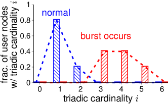
((c)) triadic cardinality dist.

Figure 1: Interaction burst and interaction triangle, in which edges in (a) and (b) represent interactions among users.

Influence triangles in user-content interactions. Similar triangle structure can also be observed in bursts caused by user-content interactions. We say that a media content piece becomes bursty if many users interact with it in a short time period. There are many reasons why a user interacts with a piece of media content. Here, we are particularly interested in the case where one user influences another user to interact with the content, a.k.a., the cascading diffusion [16] or word-of-mouth spreading [17]. It is known that many emerging news stories arising from OSNs are related to this mechanism such as the story about the killing of Osama bin Laden [18]. We find that a bursty media content piece formed by this mechanism is associated with triangle formations in a network. To illustrate this, consider Fig. 2(a), in which there are five user nodes $\{a,b,d,e,u\}$ and four content nodes $\{c_{1},c_{2},c_{3},c_{4}\}$. A directed edge between two users means that one follows another, and an undirected edge labeled with a timestamp between a user node and a content node represents an interaction between the user and the content at the labeled time. We say content node $c$ has an influence triangle if there exist two users $a,b$ such that $a$ follows $b$ and $a$ interacts with $c$ later than $b$ does. In other words, the reason $a$ interacts with $c$ is due to the influence of $b$ on $a$. In Fig. 2(a), only $c_{2}$ has an influence triangle, the others have no influence triangle, meaning that the majority of user-content interactions are not due to influence; while in Fig. 2(b), every content node is part of at least one influence triangle, meaning that many content pieces are spreading in a cascading manner in the OSN. From the perspective of an OSN manager who wants to know the operation status of the OSN, if the OSN suddenly switches to a state similar to Fig. 2(b) (from a previous state similar to Fig. 2(a)), he knows that a cascading burst is present on the network.

((a)) normal

((b)) cascading burst

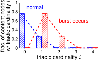
((c)) triadic cardinality dist.

Figure 2: Cascading burst and influence triangle.

Characterizing bursts. So far, we find a common structure shared by different types of bursts: the emergence of interaction bursts (caused by user-user interaction) and cascading bursts (caused by user-content interaction) are both accompanied with the formation of triangles, i.e., interaction or influence triangles, in appropriately defined networks. This finding motivates us to characterize patterns of bursts in an OSN by characterizing the triangle statistics of a network, which we called the triadic cardinality distribution.

Triadic cardinality of a node in a network, e.g., a user node in Fig. 1(a) or a content node in Fig. 2(a), is the number of triangles that it belongs to. The triadic cardinality distribution then characterizes the fractions of nodes with certain triadic cardinalities. When a burst occurs, because many new interaction/influence triangles are formed, we will observe that some nodes’ triadic cardinalities increase, and this results in the distribution “shifting” to right, as illustrated in Figs. 1(c) and 2(c). The triadic cardinality distribution provides succinct summary information to characterize burst patterns of a large scale OSN. Hence, by tracking triadic cardinality distributions, we can detect the presence of bursts.

In this paper, we assume that user interactions are aggregated chronologically to form a social activity stream, which can be considered as an abstraction of a tweet stream in Twitter, or a news feed in Facebook. We aim to calculate triadic cardinality distributions from this stream. The challenge is that when a network is large or users are active, the social activity stream will be of high speed. For example, the speed of the Twitter’s tweets stream can be as high as $5,700$ tweets per second on average, $143,199$ tweets per second during the peak time, and about $500$ million to $12$ billion tweets are aggregated per day [19]. To handle such a high-speed social activity stream, we design a sample-estimate framework, which can provide maximum likelihood estimates of the triadic cardinality distribution using sampled data. Our system works in a near-real-time fashion, and is demonstrated to be accurate and efficient.

Contributions. In this work, we make the following contributions:

• We find a useful and robust measure, triadic cardinality distribution, that can be used to characterize burst patterns of user interactions in a large OSN. It has a robustness property that is immunized against common spamming social-bot attacks.

• We design a unified sample-estimate framework that is able to provide maximum likelihood estimates of the triadic cardinality distribution. Under this framework, we study two types of stream sampling methods, and provide insights about their performance difference, through calculating the Fisher information matrices, and empirical evaluations.

• We conduct extensive experiments using real world data to demonstrate the usefulness of triadic cardinality distribution, and prove the effectiveness of our sample-estimate framework.

The remainder of the work will proceed as follows. In § II, we formally define the triadic cardinality distribution, and give an overview about our sample-estimate solution. In § III, we design two types of stream sampling methods to reduce storage complexity and improve computational efficiency. We then elaborate a maximum likelihood estimation method in § IV, and obtain the Cramér-Rao lower bound in § V. We provide detailed validations of our methods in § VI, including a real world application on detecting bursts during the 2014 Hong Kong occupy central movement. Finally, § VII summarizes some related work, and § VIII concludes.

II Problem Formulation

We first formally define the notions of social activity stream and triadic cardinality distribution mentioned in Introduction. Then we give an overview of our sample-estimate framework.

II-A Social Activity Stream

We represent an OSN by a simple graph $G=(V,E,C)$, where $V$ is a set of users, $E$ is a set of relations among users, and $C$ is a set of media content such as hashtags and video links. Here, a relation between two users can be undirected like the friend relationship in Facebook, or directed like the follower relationship in Twitter.

Users in the OSN generate social activities, e.g., interact with other users in $V$, or content in $C$. We denote a social activity by $a\in V\times(V\cup C)\times[0,\infty)$. Here user-user interaction, $a=(u,v,t)$, corresponds to user $u$ interacting with user $v$ at time $t$; and user-content interaction, $a=(u,c,t)$, corresponds to user $u$ interacting with content $c$ at time $t$. These social activities are then aggregated chronologically to form a social activity stream, denoted by $S=\{a_{1},a_{2},\ldots\}$, where $a_{l}$ denotes the $l$-th social activity in the stream.

II-B Triadic Cardinality Distribution

We introduce two interaction multigraphs formed by the two types of user interactions respectively. Triadic cardinality distribution is then defined on these two interaction multigraphs.

Interaction multigraphs. Within a time window (e.g., an hour, a day, or a week), user-user interactions in stream $S$ form a multigraph $\mathcal{G}_{\text{uu}}=(V,\mathcal{E}_{\text{uu}})$, where $V$ is the original set of users, and $\mathcal{E}_{\text{uu}}$ is a multiset consisting of user-user interactions in the window. The triadic cardinality of a user $u\in V$ is the number of interaction triangles related to $u$ in $\mathcal{G}_{\text{uu}}$. For example, user $u$ in Fig. 1(a) has triadic cardinality two, and all other users have triadic cardinality one.

Likewise, user-content interactions also form a multigraph $\mathcal{G}_{\text{uc}}=(V\cup C,E\cup\mathcal{E}_{\text{uc}})$ in a time window. Unlike $\mathcal{G}_{\text{uu}}$, the node set in $\mathcal{G}_{\text{uc}}$ includes both user nodes $V$ and content nodes $C$, and the edge set includes user relations $E$ and a multiset $\mathcal{E}_{\text{uc}}$ denoting user-content interactions in the window. Note that in $\mathcal{G}_{\text{uc}}$, triadic cardinality is only defined for content nodes, and the triadic cardinality of a content node $c\in C$ is the number of influence triangles related to $c$ in $\mathcal{G}_{\text{uc}}$. For example, in Fig. 2(a), content $c_{2}$ has triadic cardinality one, and all other content nodes have triadic cardinality zero.

Triadic cardinality distribution. Let $\theta=(\theta_{0},\ldots,\theta_{W})$ and $\vartheta=(\vartheta_{0},\ldots,\vartheta_{W^{\prime}})$ denote the triadic cardinality distributions on $\mathcal{G}_{\text{uu}}$ and $\mathcal{G}_{\text{uc}}$ respectively. Here, $\theta_{i}$ (or $\vartheta_{i}$) is the fraction of user (or content) nodes with triadic cardinality $i$ in $\mathcal{G}_{\text{uu}}$ (or $\mathcal{G}_{\text{uc}}$), and $W$ (or $W^{\prime}$) denotes the maximum triadic cardinality.

The importance of the triadic cardinality distribution lies in its capability of providing succinct summary information to characterize burst patterns in a large scale OSN as we mentioned previously. By tracking triadic cardinality distributions, we will discover burst occurrences in an OSN.

II-C Overview of Our Sample-Estimate Framework

We propose an online solution capable of tracking the triadic cardinality distribution from a high-speed social activity stream in a near-real-time fashion, as illustrated in Fig. 3.

Figure 3: A sample-estimate framework

Our system consists of two stages. In the first stage, we sample a social activity stream in a time window maintaining only summary statistics, and in the second stage, we construct an estimate of the triadic cardinality distribution from the summary statistics at the end of a time window. The advantage of this approach is that it reduces the amount of data need to be stored and processed in the system, and enables detecting bursts in a near-real-time fashion.

III Stream Sampling Methods

In this section, we elaborate the sampling module in our system, and design two types of stream sampling methods. The purpose of sampling is to reduce the computational cost in handling the massive amount of data in a high-speed stream.

III-A Identical Triangle Sampling (ITS)

The simplest stream sampling method should work as follows. We toss a biased coin for each coming social activity $a\in S$. We keep $a$ with probability $p$, and ignore it with probability $1-p$. Hence, each social activity is independently sampled, and at the end of the time window, only a fraction $p$ of the stream is kept. When social activities are sampled, triangles in graphs $\mathcal{G}_{\text{uu}}$ and $\mathcal{G}_{\text{uc}}$ are sampled accordingly. Obviously, an interaction triangle is sampled with identical probability $p^{3}$, as illustrated in Fig. 4(a).

((a)) interaction triangle

((b)) influence triangle

((c)) triangles sharing edges

Figure 4: Sampling triangles. A solid edge represents an interaction in $\mathcal{E}_{\text{uu}}\cup\mathcal{E}_{\text{uc}}$, and a dashed edge represents a social edge in $E$.

For influence triangle, we need a few more considerations. First, an influence triangle consists of two user-content interaction edges in $\mathcal{E}_{\text{uc}}$ and one social edge in $E$. Second, stream sampling only applies to edges in $\mathcal{E}_{\text{uc}}\cup\mathcal{E}_{\text{uu}}$, and edges in $E$ are not sampled because they do not appear in the stream. In Fig. 4(b), suppose we have sampled two user-content interactions $(u,c,t_{1})$ and $(v,c,t_{2})$, and assume $t_{1}\leq t_{2}$, i.e., user $u$ interacts with $c$ earlier than $v$. To determine whether content $c$ has an influence triangle formed by users $u$ and $v$, we need to check whether (directed) edge $(v,u)$ exists in $E$. This can be done by querying neighbors of one of the two users in the OSN. For example, in Twitter, we query followees of $v$ and check whether $v$ follows $u$; or in Facebook, we query friends of $v$ and check whether $u$ is a friend of $v$. Sometimes this query cost is expensive if we do not own $G$ and need to call the API provided by the OSN. To reduce this query cost, we check a user pair with probability $p^{\prime}$. This is equivalent to sampling a social edge in $E$ with probability $p^{\prime}$, conditioned on the two associated user-content interactions having been sampled. Thus, an influence triangle is sampled with identical probability $p^{2}p^{\prime}$. In summary, we have the following result.

Theorem 1.

If we independently sample each social activity in stream $S$ with probability $p$, and check a user relation in $E$ with probability $p^{\prime}$, then each interaction (influence) triangle in $\mathcal{G}_{\text{uu}}$ ($\mathcal{G}_{\text{uc}}$) is sampled with identical probability

$$p_{\triangle}^{\text{ITS}}=\begin{cases}p^{3}&\text{for an interaction triangle},\\ p^{2}p^{\prime}&\text{for an influence triangle}.\end{cases}$$ (1)

A more efficient ITS method. An obvious drawback of the previous sampling method is that an interaction triangle is sampled with probability cubic to the edge sampling probability. This means that an interaction triangle is hardly sampled if $p$ is too small. In fact, we can increase triangle sampling probability to $p^{2}$ (and still keep each edge being sampled with probability $p$) by leveraging a clever colorful triangle sampling method [20]. Let $N=1/p$ be an integer, and $[N]$ represents a set of $N$ colors. Define a hash function $h\colon V\mapsto[N]$ that maps a node to one of these $N$ colors uniformly at random. During sampling, for a coming social activity $a=(u,v,t)$, we keep $a$ if $h(u)=h(v)$, and drop $a$ otherwise. We can see that a user-user interaction is still sampled with probability $p$, but an interaction triangle is now sampled with probability $p^{2}$, and hence it is more efficient in collecting triangles from edge samples. For influence triangle, we can let $p^{\prime}=1$, i.e., we check every sampled user pair (similar to gSH [21]), and an influence triangle is also sampled with probability $p^{2}$. We will refer to ITS method with colorful triangle sampling as ITS-color in the following discussion.

Remark In both ITS and ITS-color, although triangles are sampled identically, they may not be sampled independently, such as the cases two triangles share edges in Fig. 4(c). We will consider this issue in detail later.

III-B Harvesting Triangles by Subgraph Sampling (SGS)

The ITS based methods are easy to implement, and they are already used for counting the triangles in a large network [22, 20]. However, ITS based methods have drawbacks when they are used for estimating the triadic cardinality distribution. One main drawback is that, because ITS samples each triangle with identical probability, the sampling will be biased towards nodes belonging to many triangles. That is, nodes with larger triadic cardinalities are more likely to be sampled, and for nodes with small triadic cardinalities, the triangles these nodes belonging to will be seldom sampled. This hence may incur large estimation error for nodes with small triadic cardinalities. To address this weakness, we propose another triangle sampling method that leverages interaction multigraphs and social graph in a different way, which we call the subgraph sampling (SGS) method.

For interaction triangle, assume that we are only interested in user-user interactions along social edges. Then SGS works as follows. At the beginning of a time window, we first sample a set of user samples that each user is sampled with probability $p_{n}$ (and this step can be independently implemented on social graph $G$ using well-studied graph sampling techniques [23]). For each sampled user, a subgraph induced by the user and the user’s neighbors in $G$ is maintained, i.e., each edge in the induced subgraph is an social edge in $G$. During stream sampling, for each social activity $a=(u,v,t)$, if $(u,v)$ is an edge in one of these subgraphs, we keep $a$; otherwise $a$ is dropped. In this way, interaction triangles related to the user sample are kept completely.

Similar procedure is also applied to sample influence triangles, and here we aim to keep complete influence triangles related to each sampled content node. To sample a content node with probability $p_{n}$, we need to store content nodes seen so far in a Bloom filter for ease of testing whether a coming content node is new or not. For a coming social activity $a=(u,c,t)$, if $c$ is already marked as a sampled content node, we keep $a$; if $c$ is new (i.e., $c$ is not found in the Bloom filter), we mark $c$ as a content node sample with probability $p_{n}$ and save $a$, otherwise we drop $a$. No matter $a$ is saved or discarded, if $c$ is new, we need to store $c$ in the Bloom filter. So, we can see that social activities related to sampled content nodes are all kept, if we also check the existence of social edges with probability $p^{\prime}=1$, then influence triangles related to sampled content nodes are kept completely.

SGS method thus keeps every triangle a node sample belonging to, whatever the node sample has large or small triadic cardinality. We will later develop rigorous method to compare the performance of ITS based methods and SGS method.

III-C Statistics of Sampled Data

Both ITS (including ITS-color) and SGS can be thought of as sampling edges in multigraphs $\mathcal{G}_{\text{uu}}$, $\mathcal{G}_{\text{uc}}$, and social graph $G$, in different manners. In ITS, interaction edges $e\in\mathcal{E}_{\text{uu}}\cup\mathcal{E}_{\text{uc}}$ are independently sampled with probability $p$, and social edges $e^{\prime}\in E$ are sampled with conditional probability $p^{\prime}$. In SGS, we first sample a collection of user/content nodes with probability $p_{n}$, and then only keep triangles related to these sampled user/content nodes.

At the end of the time window, we obtain two sampled multigraphs $\mathcal{G}_{\text{uu}}^{\prime}$ and $\mathcal{G}_{\text{uc}}^{\prime}$. Calculating the triadic cardinalities for nodes in these smaller graphs is much efficient than on the original graphs. For the sampled graph $\mathcal{G}_{\text{uu}}^{\prime}$, we calculate triadic cardinality for each (sampled) user node in ITS (SGS), and obtain statistics $g=(g_{0},\ldots,g_{W})$, where $g_{j}$, $0\leq j\leq W$, denotes the number of user nodes belonging to $j$ triangles in graph $\mathcal{G}_{\text{uu}}^{\prime}$. Similar statistics are also obtained from $\mathcal{G}_{\text{uc}}^{\prime}$, denoted by $f=(f_{0},\ldots,f_{W^{\prime}})$ (where $f_{j}$ is the number of content nodes belonging to $j$ influence triangles in graph $\mathcal{G}_{\text{uc}}^{\prime}$). We only need to store $g$ and $f$ in main memory and use them to estimate $\theta$ and $\vartheta$ in the next section.

IV Maximum Likelihood Estimate

In this section, we elaborate the estimation module in our system, and derive a maximum likelihood estimate (MLE) of the triadic cardinality distribution using statistics obtained in the sampling step. The estimation in this section can be viewed as an analog of the network flow size distribution estimation [24, 25, 26, 27, 28], in which a packet in a flow is viewed to be a triangle a node belonging to. However, in our case, triangle samples are not independent, and a node may have no triangles at all. These issues complicate the estimation design, and we will describe how to solve these issues in this section.

Note that we only discuss how to estimate $\theta$ using $g$, as the MLE of $\vartheta$ using $f$ is easily obtained using a similar approach. To estimate $\theta$, we first consider the easier case where graph size $|V|=n$ is known. Later, we extend our analysis to the case where $|V|$ is unknown.

IV-A A General MLE Framework when Graph Size is Known

Recall that $g_{j}$, $0\leq j\leq W$, is the number of nodes having $j$ sampled triangles in graph $\mathcal{G}_{\text{uu}}^{\prime}$. First, note that observing a node with $j$ sampled triangles in graph $\mathcal{G}_{\text{uu}}^{\prime}$ implies that the node has at least $j$ triangles in graph $\mathcal{G}_{\text{uu}}$. Second, we also need to pay special attention to $g_{0}$, which is the number of nodes with no triangle observed in graph $\mathcal{G}_{\text{uu}}^{\prime}$. Due to sampling, some nodes may be unobserved (e.g., no edge attached to the node is sampled in ITS, or the node is not sampled in SGS), and these “evaporated” nodes are actually “observed” to have zero triangle because graph $\mathcal{G}_{\text{uu}}$ has $n$ nodes. Hence, we need to include these evaporated nodes in $g_{0}$, i.e.,

$$g_{0}\coloneqq g_{0}+n-\sum_{j=0}^{W}g_{j}=n-\sum_{j=1}^{W}g_{j}.$$

To derive a MLE of $\theta$, we use a conditional probability to model the sampling process. For a randomly chosen node, let $X$ denote the number of triangles to which it belongs in $\mathcal{G}_{\text{uu}}$, and let $Y$ denote the number of triangles observed during sampling. Let $b_{ji}\triangleq P(Y=j|X=i)$ for $0\leq j\leq i$ be the conditional probability that a node has $j$ sampled triangles in $\mathcal{G}_{\text{uu}}^{\prime}$ given that it has $i$ triangles in the original graph $\mathcal{G}_{\text{uu}}$. Then the probability of observing a node to have $j$ sampled triangles is

$$P(Y=j)\!=\!\sum_{i=j}^{W}P(Y=j|X=i)P(X=i)\!=\!\sum_{i=j}^{W}b_{ji}\theta_{i}.$$ (2)

Then, the log-likelihood of observations $\{Y_{l}=y_{l}\}_{k=1}^{n}$, where $Y_{l}=y_{l}$ denotes the $k$-th node having $y_{l}$ sampled triangles, yields

$$\mathcal{L}(\theta)\triangleq\log P(\{Y_{l}=y_{l}\}_{k=1}^{n})=\sum_{j=0}^{W}g_{j}\log\sum_{i=j}^{W}b_{ji}\theta_{i}.$$ (3)

The MLE of $\theta$ can then be obtained by maximizing $\mathcal{L}(\theta)$ with respect to $\theta$ under the constraint that $\sum_{i=0}^{W}\theta_{i}=1$. To solve the likelihood maximization problem, we face two challenges: (1) What are the specific formulas of $b_{ji}$ for the sampling methods we have proposed previously? (2) Note that it is impossible to obtain a closed form solution maximizing Eq. (3), so how should we design an algorithm to maximize Eq. (3) conveniently?

IV-A1 Sampling Model Specification

We specify the sampling models $b_{ji}$ for ITS and SGS, respectively. We start with SGS for its simplicity.

SGS: Remember that SGS keeps all the triangles of each sampled node, and a node is sampled with probability $p_{n}$. Hence, if we observe a node belonging to $j>0$ triangles in $\mathcal{G}_{\text{uu}}^{\prime}$, the node must have $i=j$ triangles in $\mathcal{G}_{\text{uu}}$, and this occurs with probability $p_{n}$. If we observe a node having no triangle in $\mathcal{G}_{\text{uu}}^{\prime}$, i.e., $j=0$, there are two possibilities, i.e., the node indeed has no triangle in $\mathcal{G}_{\text{uu}}$, $i=0$, or the node is not sampled. Therefore,

$$b_{ji}=\begin{cases}1,&\text{if }j=i=0,\\ 1-p_{n},&\text{if }j=0\wedge i>0,\\ p_{n},&\text{if }j=i,\\ 0,&\text{otherwise}.\end{cases}$$

ITS and ITS-color: In ITS or ITS-color, each triangle is sampled with identical probability, denoted by $p_{\triangle}$. Sampling a triangle can be thought of as a Bernoulli trial with success probability $p_{\triangle}$. If Bernoulli trials are independent, meaning that triangles are independently sampled, then $b_{ji}=P(Y=j|X=i)$ should follow the standard binomial distribution parameterized by $i$ and $p_{\triangle}$. Unfortunately, independence does not hold for triangles sharing edges, as illustrated in Fig. 4(c). As a result, it is non-trivial to derive an accurate sampling model $b_{ji}$ for ITS and ITS-color due to the dependence among triangle samples. To deal with this issue, we propose to approximate the sums of dependent Bernoulli random variables by a Beta-binomial distribution [29, 30], which is given by

$$\text{BetaBin}(j|i,p_{\triangle},\alpha)$$

$$\triangleq\binom{i}{j}\frac{\prod_{s=0}^{j-1}(s\alpha+p_{\triangle})\prod_{s=0}^{i-j-1}(s\alpha+1-p_{\triangle})}{\prod_{s=0}^{i-1}(s\alpha+1)}$$

and $\prod_{0}^{-1}\triangleq 1$. The above distribution parameterized by $\alpha\geq 0$ allows pairwise identically distributed Bernoulli random variables to have covariance $\alpha p_{\triangle}(1-p_{\triangle})/(1+\alpha)$. It reduces to the standard binomial distribution when $\alpha=0$. Hence, for ITS and ITS-color, the sampling model is approximated by

$$b_{ji}(\alpha)=\text{BetaBin}(j|i,p_{\triangle},\alpha),\quad j\in[0,i].$$

IV-A2 MLE via EM Algorithm

To solve the second challenge, we propose to use the expectation-maximization (EM) algorithm to obtain the MLE in a more convenient way. For general consideration, we use $b_{ji}(\alpha)$ to denote the sampling model.

If we already know that the $k$-th node has $x_{l}$ triangles in $\mathcal{G}_{\text{uu}}$, i.e., $X_{l}=x_{l}$, then the complete likelihood of observations $\{(Y_{l},X_{l})\}_{l=1}^{n}$ is

$$P(\{(Y_{l},X_{l})\}_{l=1}^{n})=\prod_{l=1}^{n}P(Y_{l}=y_{l},X_{l}=x_{l})$$

$$=\prod_{j=0}^{W}\prod_{i=j}^{W}P(Y=j,X=i)^{z_{ij}}=\prod_{j=0}^{W}\prod_{i=j}^{W}\left[b_{ji}(\alpha)\theta_{i}\right]^{z_{ij}}$$

where $z_{ij}=\sum_{l=1}^{n}\mathbf{1}(x_{l}=i\wedge y_{l}=j)$ is the number of nodes with $i$ triangles and $j$ of them being sampled; $\mathbf{1}(\cdot)$ is the indicator function. The complete log-likelihood is

$$\mathcal{L}_{c}(\theta,\alpha)\triangleq\sum_{j=0}^{W}\sum_{i=j}^{W}z_{ij}\log\left[b_{ji}(\alpha)\theta_{i}\right].$$ (4)

Here, we can treat $\{X_{l}\}_{l=1}^{n}$ as hidden variables, and apply the EM algorithm to calculate the MLE.

E-step. We calculate the expectation of the complete log-likelihood in Eq. (4) with respect to hidden variables $\{X_{l}\}_{l}$, conditioned on data $\{Y_{l}\}_{l}$ and previous estimates $\theta^{(t)}$ and $\alpha^{(t)}$. That is

$$Q(\theta,\alpha;\theta^{(t)},\alpha^{(t)})\triangleq\sum_{j=0}^{W}\sum_{i=j}^{W}\mathbb{E}[z_{ij}|\theta^{(t)},\alpha^{(t)}]\log\left[b_{ji}(\alpha)\theta_{i}\right].$$

Here, $\mathbb{E}[z_{ij}|\theta^{(t)},\alpha^{(t)}]$ can be viewed as the average number of nodes that have $i$ triangles in $\mathcal{G}_{\text{uu}}$, of which $j$ are sampled. Because

$$P(X=i|Y=j,\theta^{(t)},\alpha^{(t)})$$

$$=\frac{P(Y=j|X=i,\alpha^{(t)})P(X=i|\theta^{(t)})}{\sum_{i^{\prime}}P(Y=j|X=i^{\prime},\alpha^{(t)})P(X=i^{\prime}|\theta^{(t)})}$$

$$=\frac{b_{ji}(\alpha^{(t)})\theta_{i}^{(t)}}{\sum_{i^{\prime}}b_{ji^{\prime}}(\alpha^{(t)})\theta_{i^{\prime}}^{(t)}}\triangleq p_{i|j}$$

and we have observed $g_{j}$ nodes belonging to $j$ sampled triangles, then $\mathbb{E}[z_{ij}|\theta^{(t)},\alpha^{(t)}]=g_{j}p_{i|j}$.

M-step. We now maximize $Q(\theta,\alpha;\theta^{(t)},\alpha^{(t)})$ with respect to $\theta$ and $\alpha$ subject to the constraint $\sum_{i=0}^{W}\theta_{i}=1$. After the $\log$ operation, $\theta$ and $\alpha$ are well separated. Hence, we obtain

$$\theta_{i}^{(t+1)} =\arg\max_{\theta}Q(\theta,\alpha;\theta^{(t)},\alpha^{(t)})$$

$$=\frac{\sum_{j=0}^{i}\mathbb{E}[z_{ij}|\theta^{(t)},\alpha^{(t)}]}{\sum_{j=0}^{W}\sum_{i^{\prime}=j}^{W}\mathbb{E}[z_{i^{\prime}j}|\theta^{(t)},\alpha^{(t)}]},\quad 0\leq i\leq W,$$

and $\alpha^{(t+1)}=\arg\max_{\alpha}Q(\theta,\alpha;\theta^{(t)},\alpha^{(t)})$ can be solved using classic gradient ascent methods.

Alternating iterations of the E-step and M-step, EM algorithm converges to a solution, which is a local maximum of $\mathcal{L}(\theta,\alpha)$. We denote this solution by $\hat{\theta}$ and $\hat{\alpha}$.

IV-B MLE when Graph Size is Unknown

When the graph size is unknown, one can use probabilistic counting methods such as loglog counting [31] to obtain an estimate of graph size from the stream, and then apply our previously developed method to obtain estimate $\hat{\theta}$. Note that this introduces additional statistical errors to $\hat{\theta}$ due to the inaccurate estimate of the graph size. In what follows, we slightly reformulate the problem and develop a method that can simultaneously estimate both the graph size and the triadic cardinality distribution from the sampled data.

When the graph size is unknown, we cannot calibrate $g_{0}$ because “evaporated” nodes are indeed unobservable in this case. There is no clear relationship between an unsampled node and its triadic cardinality. As a result, we cannot easily model the absence of nodes by $\theta$. If we observe a node having no triangle after sampling, we cannot reason out which way caused the observation, the node has no triangle in the original graph, or the triangles the node belonging to are not sampled. This difficulty hence complicates the estimation design.

To solve this issue, we need to slightly reformulate our problem: (1) Instead of estimating the total number of nodes in $\mathcal{G}_{\text{uu}}$, we estimate the number of nodes belonging to at least one triangle in $\mathcal{G}_{\text{uu}}$, denoted by $n_{+}$; (2) We estimate the triadic cardinality distribution $\theta^{+}=(\theta_{1}^{+},\ldots,\theta_{W}^{+})$, where $\theta_{i}^{+}$ is the fraction of nodes with $i$ triangles over the nodes having at least one triangle in $\mathcal{G}_{\text{uu}}$.

Estimating $n_{+}$. Under the Beta-binomial model, the probability that a node has $i$ triangles in $\mathcal{G}_{\text{uu}}$, of which none are sampled, is

$$q_{i}(\alpha)\triangleq P(Y=0|X=i)=b_{0i}(\alpha).$$

Then, the probability that a node has triangles in $\mathcal{G}_{\text{uu}}$, of which none are sampled, is

$$q(\theta^{+},\alpha)\triangleq P(Y=0|X\geq 1)=\sum_{i=1}^{W}q_{i}(\alpha)\theta_{i}^{+}.$$

Because there are $\sum_{j=1}^{W}g_{j}$ nodes having been observed to have at least one sampled triangle, $n_{+}$ can be estimated by

$$\hat{n}_{+}=\frac{\sum_{j=1}^{W}g_{j}}{1-q(\theta^{+},\alpha)}.$$ (5)

Note that estimator (5) relies on $\theta^{+}$ and $\alpha$, and we can estimate them using the following procedures.

Estimating $\theta^{+}$ and $\alpha$. We discard $g_{0}$ and only use $g^{+}\triangleq(g_{1},\ldots,g_{W})$ to estimate $\theta^{+}$ and $\alpha$. The basic idea is to derive the likelihood for nodes that are observed to have at least one sampled triangle, i.e., $\{Y_{l}=y_{l}\colon y_{l}\geq 1\}$. In this case, the probability that a node has $X=i$ triangles, and $Y=j$ of them are sampled, conditioned on $Y\geq 1$, is

$$P(Y=j|X=i,Y\geq 1) =\frac{P(Y=j|X=i)}{P(Y\geq 1|X=i)}$$

$$=\frac{b_{ji}(\alpha)}{1-q_{i}(\alpha)}\triangleq a_{ji}(\alpha),\quad j\geq 1.$$

Then the probability that a node is observed to have $j$ sampled triangles, conditioned on $Y\geq 1$, is

$$P(Y=j|Y\geq 1)$$

$$=\sum_{i=j}^{W}P(Y=j|X=i,Y\geq 1)P(X=i|Y\geq 1)$$

$$=\sum_{i=j}^{W}a_{ji}(\alpha)\phi_{i},$$

where

$$\phi_{i}\triangleq P(X=i|Y\geq 1)=\frac{\theta_{i}^{+}[1-q_{i}(\alpha)]}{\sum_{i^{\prime\prime}=1}^{W}\theta_{i^{\prime}}^{+}[1-q_{i^{\prime}}(\alpha)]},$$ (6)

is the distribution of observed node triadic cardinalities. Now it is straightforward to obtain the previously mentioned likelihood. Furthermore, we can leverage our previously developed EM algorithm by replacing $\theta_{i}$ by $\phi_{i}$, $b_{ji}$ by $a_{ji}$, to obtain MLEs for $\phi$ and $\alpha$. We omit these details, and directly provide the final EM iterations:

$$\phi_{i}^{(t+1)}=\frac{\sum_{j=1}^{i}\mathbb{E}[z_{ij}|\phi^{(t)},\alpha^{(t)}]}{\sum_{j=1}^{W}\sum_{i^{\prime}=j}^{W}\mathbb{E}[z_{i^{\prime}j}|\phi^{(t)},\alpha^{(t)}]},\quad i\geq 1,$$

where

$$\mathbb{E}[z_{ij}|\phi^{(t)},\alpha^{(t)}]=\frac{g_{j}a_{ji}(\alpha^{(t)})\phi_{i}^{(t)}}{\sum_{i^{\prime}=j}^{W}a_{ji^{\prime}}(\alpha^{(t)})\phi_{i^{\prime}}^{(t)}},\quad i\geq j\geq 1,$$

and $\alpha^{(t+1)}=\arg\max_{\alpha}Q(\phi,\alpha;\phi^{(t)},\alpha^{(t)})$ is solved using gradient ascent methods.

Once EM converges, we obtain estimates $\hat{\phi}$ and $\hat{\alpha}$. The estimate for $\theta^{+}$ is then obtained by Eq. (6), i.e.,

$$\hat{\theta}_{i}^{+}=\frac{\hat{\phi}_{i}/[1-q_{i}(\hat{\alpha})]}{\sum_{i^{\prime}=1}^{W}\hat{\phi}_{i^{\prime}}/[1-q_{i^{\prime}}(\hat{\alpha})]},\quad 1\leq i\leq W.$$ (7)

Finally, $\hat{n}_{+}$ is obtained by the estimator in Eq. (5).

IV-C Logarithmic Binning Simplification

In our previous study [32], we have observed that triadic cardinality distributions in many real-world networks exhibit heavy tails. Thus, it is better to characterize them in the logarithmic scale. That is, instead of estimating the fraction of nodes having exact triadic cardinality $i$, we may want to estimate the fraction of nodes with triadic cardinality in $\log_{2}$ scaled bins. We aim to estimate the fraction of nodes having triadic cardinality in the $k$-th bin $[2^{k},2^{k+1})$, denoted by $\theta^{+}_{k}$, for $k=0,1,\ldots,K$ where $K\triangleq\lfloor\log_{2}W\rfloor$. If we allow $i=0$ as in the case where graph size is known, we define the first bin to be $\{0\}$ assigning to bin $k=-1$, and use $\theta_{k},k=-1,0,\ldots,K$, to represent the binned triadic cardinality distribution.

In the logarithmic binning simplification, for each $i$ in the $k$-th bin, we assume that $\theta_{i}$ has the same value, and $\theta_{i}=2^{-k}\theta_{k}$ for $k\geq 0$. We further define

$$b_{jk} \triangleq P(Y=j|X\in\text{bin}(k))$$

$$=\sum_{i=2^{k}}^{2^{k+1}-1}P(Y=j|X=i)P(X=i|X\in\text{bin}(k))$$

$$=2^{-k}\sum_{i=2^{k}}^{2^{k+1}-1}b_{ji}$$

for $k\geq 0$. For $k=-1$, we define $b_{jk}=1$ if $j=0$ and $0$ otherwise. Similar to Eq. (2), the probability of observing a node having $j$ triangles after sampling becomes $P(Y=j)=\sum_{k=-1}^{K}b_{jk}\theta_{k}$. Thus, it is straightforward to obtain a MLE of $\theta_{k}$ using previously developed methods. Similar analysis can also be applied to estimate $\theta_{k}^{+}$, and hence is omitted.

The logarithmic binning simplification reduces the number of parameters from $W+1$ to $\lfloor\log_{2}W\rfloor+1$ that allows us to consider large triadic cardinality bound $W$ in large networks. Meanwhile, $\{\theta_{k}\}$ and $\{\theta_{k}^{+}\}$ are actually smoothed versions of $\{\theta_{i}\}$ and $\{\theta_{i}^{+}\}$, which we will observe in experiments.

V Asymptotic Estimation Error Analysis

To evaluate the performance of MLEs using different sampling methods, this section devotes to analyze the asymptotic estimation error of the MLEs by calculating the Cramér-Rao lower bound (CRLB) of $\hat{\theta}$ and $\hat{\theta}^{+}$. It is well-known that MLE is asymptotically Gaussian centered at the true value with variance the CRLB, and the Cramér-Rao theorem further states that the mean squared error of any unbiased estimator is lower bounded by the CRLB, which is the inverse of the Fisher information (see [33, Chapter 2] for more details).

Intuitively, the Fisher information can be thought of as the amount of information that observations $\{Y_{l}\}$ carry about unobservable parameters $\theta$ (or $\theta^{+}$) upon which the probability distribution of the observations depends. When graph size is known, the Fisher information of observations $\{Y_{l}\}$ is a $(W+1)\times(W+1)$ square matrix $J(\theta)$ whose $ir$-th element is given by

$$J_{ir}(\theta)\triangleq\mathbb{E}_{Y}\left[\frac{\partial\log P(\{Y_{l}\}_{l}|\theta)}{\partial\theta_{i}}\frac{\partial\log P(\{Y_{l}\}_{l}|\theta)}{\partial\theta_{r}}\right].$$

In our problem, $J_{ir}(\theta)$ can be further simplified to

$$J_{ir}(\theta) =n\sum_{j=0}^{W}\frac{\partial\log P(Y|\theta)}{\partial\theta_{i}}\frac{\partial\log P(Y|\theta)}{\partial\theta_{r}}P(Y=j)$$

$$=n\sum_{j=0}^{W}\frac{b_{ji}(\alpha)b_{jr}(\alpha)}{P(Y=j)}.$$

When graph size is unknown, the Fisher information matrix $J(\theta^{+})$ is a $W\times W$ matrix. To obtain $J(\theta^{+})$, we can first obtain the Fisher information matrix regarding to $\phi$, denoted by $J(\phi)$, using an approach similar to above (by replacing $n$ by $n^{+}$). Then $J(\phi)$ and $J(\theta^{+})$ are known to have the following relationship [34]

$$J(\theta^{+})^{-1}=\nabla HJ(\phi)^{-1}\nabla H^{T},$$

where $\nabla H$ is the Jacobian matrix, and its $ir$-th element is given by $\partial\theta_{i}^{+}(\phi)/\partial\phi_{r}$ (and $\theta_{i}^{+}(\phi)$ is given by Eq. (7)).

The inverse constrained Fisher information of $\theta$ with constraint $\sum_{i}\theta_{i}=1$ is then obtained by

$$I(\theta)=J(\theta)^{-1}-\theta\theta^{T},$$

where the term $\theta\theta^{T}$ corresponds to the accuracy gain due to constraint $\sum_{i}\theta_{i}=1$ (see [35, 26] for more details). Then, mean squared error of an estimator $\hat{\theta}$ is lower bounded by the diagonal elements of $I(\theta)$, i.e., $\mathbb{E}[(\hat{\theta}_{i}-\theta_{i})^{2}]\geq I_{ii}(\theta)$. Similar relation also holds for $\hat{\theta}^{+}$.

MLE is asymptotically efficient, and CRLB is its asymptotic variance. We are thus able to leverage CRLB to compare the asymptotic estimation accuracy of MLEs using different sampling methods.

VI Experiments and Validations

In this section, we first empirically verify the claims we have made previously. Then, we validate the proposed estimation methods on several real-world networks. Finally, we illustratively show the usefulness of triadic cardinality distribution in detecting bursts during the Hong Kong Occupy Central movement in Twitter.

VI-A Analyzing Bursts in Enron Dataset

In the first experiment, we use a public email communication dataset to empirically show how bursts in networks can change the triadic cardinality distribution, and verify our claims previously made.

VI-A1 Enron email dataset

The Enron email dataset [36] includes the entire email communications (e.g., who sent an email to whom at what time) of the Enron corporation from its startup to bankruptcy. The used dataset is carefully cleaned by removing spamming accounts/emails and emails with incorrect timestamps. The cleaned dataset contains $22,477$ email accounts and $164,081$ email communications between Jan 2001 and Apr 2002. We use this dataset to study patterns of bursts caused by email communications among people, i.e., by user-user interactions.

VI-A2 Observations from data

Because the data has been cleaned, the number of user-user interactions, i.e., number of sent emails per time window, reliably indicates burst occurrences. We show the number of emails sent per week in Fig. 5, and observe at least two bursts that occurred in Jun and Oct 2001, respectively. We also show the number of interaction triangles formed during each week. The Pearson correlation coefficient (PCC) between the email and triangle volum series is $0.8$, which reflects a very strong correlation. The sudden increase (or decrease) of email volumes during the two bursts is accompanied with the sudden increase (or decrease) of the number of triangles. Thus, this observation verifies our claim that the emergence of a burst is accompanied with the formation of triangles in networks.

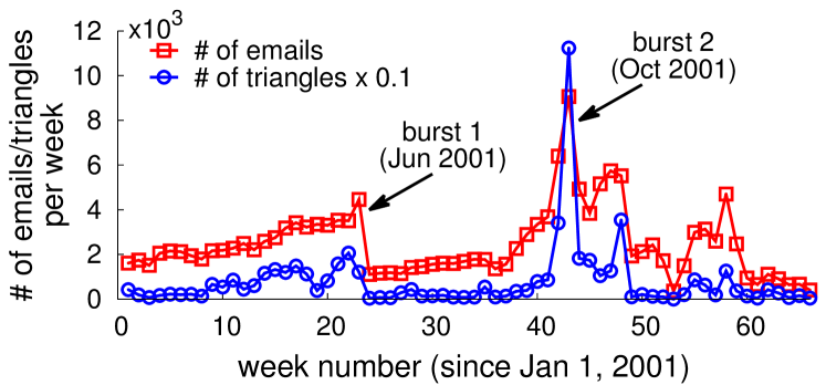
Figure 5: Email and triangle volumes per week

How bursts change triadic cardinality distributions. Our burst detection method relies on a claim that, when a burst occurs, the triadic cardinality distribution changes. To see this, we show the triadic cardinality distributions before and during the bursts in Fig. 6. For the first burst, due to the sudden decrease of email communications from week 23 to week 24, we observe in Fig. 6(a) that the distribution “shifts” to the left. While for the second burst, due to the gradual increase of email communications, we observe in Fig. 6(b) that the distribution in week 43 shifts to the right in comparison to previous weeks. Again, the observation verifies our claim that triadic cardinality distribution changes when a burst occurs.

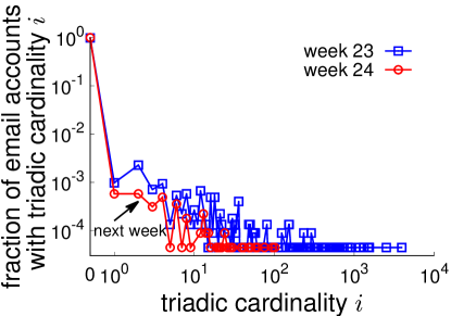
((a)) Burst 1 “shifts” the dist. to left

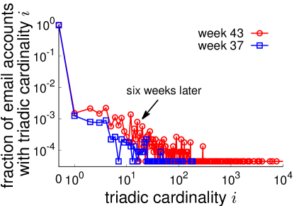
((b)) Burst 2 “shifts” the dist. to right

Figure 6: Bursts change distribution curves. For burst 1 (burst 2), the probability mass at $i=0$ slightly increases (decreases) actually.

Impacts of spam. As we mentioned earlier, if spam exists, simply using the volume of user interactions to detect bursts will result in false alarms, while the triadic cardinality distribution is a good indicator immune to spam. To demonstrate this claim, suppose a spammer suddenly becomes active in week 23, and generates email spams to distort the original triadic cardinality distribution of week 23. We consider the following two spamming strategies:

• Random: The spammer randomly chooses many target users to send spam.

• Random-Friend: At each step, the spammer randomly chooses a user and a random friend of the user, as two targets; and sends spams to each of these two targets. The spammer repeats this step a number of times.

In order to measure the extent that spams can distort the original triadic cardinality distribution of week 23, we use Kullback-Leibler (KL) divergence to measure the difference between the original and distorted distributions. The relationship between KL divergence and the number of injected spams is shown in Fig. 7(a). For both strategies, KL divergences both increase as more spams are injected into the interaction network, which is expected. The Random-Friend strategy can cause larger divergences than the Random strategy, as Random-Friend strategy is easier to introduce new triangles to the interaction network of week 23 for the reason that two friends are more likely to communicate in a week. However, even when $10^{4}$ spams are injected, the spams incur an increasing KL divergence of less than $0.04$. From Fig. 7(b), we can see that the divergence is indeed small. (This may be explained by the “center of attention” phenomenon [37], i.e., a person may have hundreds of friends but he usually only interacts with a small fraction of them in a time window. Hence, Random-Friend strategy does not form many triangles.) Therefore, these observations verify that triadic cardinality distribution is robust against common spamming attacks.

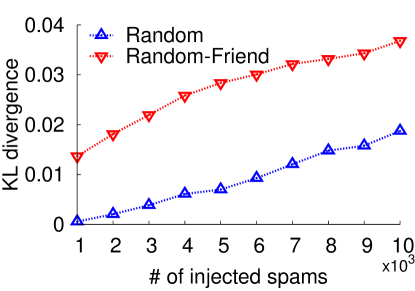
((a)) KL divergence

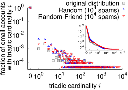
((b)) Distorted distributions

Figure 7: Impacts of spam. In (b), the inset shows fitted curves of the three distributions.

VI-B Validating Estimation Performance

In the second experiment, we evaluate the MLE performance using different sampling methods and demonstrate the computational efficiency.

VI-B1 Datasets

Because the input of our estimation methods is actually a sampled graph, we use public available graphs of different types and scales from the SNAP graph repository (http://snap.stanford.edu/data) as our testbeds. We summarize the statistics of these graphs in Table I.

TABLE I: Network statistics

Network	Type	Nodes	Edges
HepTh	directed, citation	$27,770$	$352,807$
DBLP	undirected, coauthor	$317,080$	$1,049,866$
YouTube	undirected, OSN	$1,134,890$	$2,987,624$
Pokec	directed, OSN	$1,632,803$	$30,622,564$

For each graph, we first shuffle the edges to form a stream, then we apply stream sampling methods on the stream, and obtain a sampled graph. We calculate the triadic cardinality for nodes in the sampled graph, and obtain statistics $g$. Note that the estimator uses $g$ to obtain an estimate of the triadic cardinality distribution for each graph, which is then compared with the ground truth distribution, i.e., the triadic cardinality distribution of the original unsampled graph, to evaluate the performance of the estimation method.

VI-B2 CRLB analysis

Our goal is to compare the amount of information contained in edge samples collected using different sampling methods, in terms of CRLB. A small CRLB indicates small asymptotic variance of a MLE, and hence implies that the corresponding sampling method is efficient in gathering information from data. We will mainly use the HepTh and DBLP networks in this study, and for ease of conducting matrix algebra, we truncate the stream with $W=20$ by discarding edges that may increase a node’s triadic cardinality to larger than $20$.

We depict the results when graph size is known in Fig. 8. In LABEL:sub@f:crlb_its_1 and LABEL:sub@f:crlb_its_2, we show the rooted CRLB of ITS and ITS-color with different triangle sampling rates $p_{\triangle}$ on the two networks respectively. As expected, when $p_{\triangle}$ increases, CRLB decreases, indicating that we can obtain more accurate estimates by increasing edge sampling rate. However, we find that ITS and ITS-color are not efficient in gathering information from data. As we can see, to decrease CRLB to less than $0.1$, we need to increase $p_{\triangle}$ to about $0.6$, which corresponds to a very large edge sampling rate! We then study the performance of SGS in LABEL:sub@f:crlb_sgs_1 and LABEL:sub@f:crlb_sgs_2. We observe that CRLB decreases when $p_{n}$ increases, i.e., when more nodes (or subgraphs) are sampled. We also observe that CRLB of SGS is much smaller than ITS, even with small $p_{n}$. It seems that SGS is more efficient in gathering information from data than ITS. However, people may argue that SGS may sample more edges than ITS even with small $p_{n}$. To compare them fairly, we need to fix the number of edge samples used by different methods. In ITS or ITS-color, if the graph contains $m$ edges, then ITS or ITS-color samples $mp$ edges on average. In SGS, because a randomly chosen node has $\sum_{i}i\theta_{i}$ triangles, then approximately, SGS samples $\Theta(np_{n}\sum_{i}i\theta_{i})$ edges on average (if we assume $\text{\#edges}=\Theta(\text{\#triangles})$). In the experiment, we turn $p_{\triangle}$ and $p_{n}$ to make sure that different methods indeed use same amounts of edge samples approximately, and show the results in LABEL:sub@f:crlb_cmp_1 and LABEL:sub@f:crlb_cmp_2. We can see clearly that SGS is indeed more efficient than ITS and ITS-color. ITS-color is also more efficient than ITS since ITS-color samples a triangle with larger probability than ITS using same edge sampling rate.

We also conduct same experiments when graph size is unknown, and the results are depicted in Fig. 9. The observations are consistent with the results when graph size is known.

HepTh	DBLP

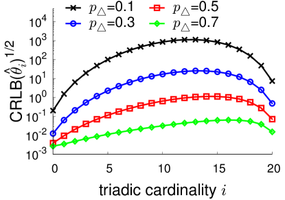
((a)) ITS (ITS-color)

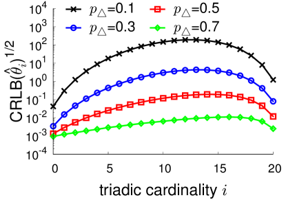
((b)) ITS (ITS-color)

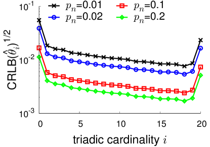
((c)) SGS

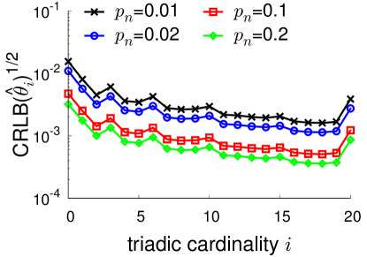
((d)) SGS

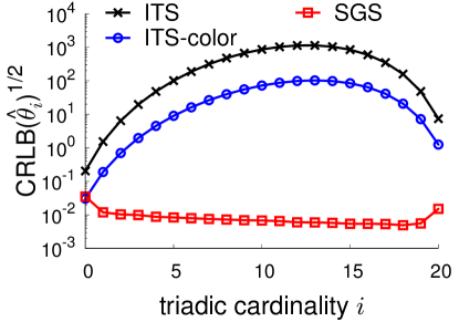
((e)) comparisons

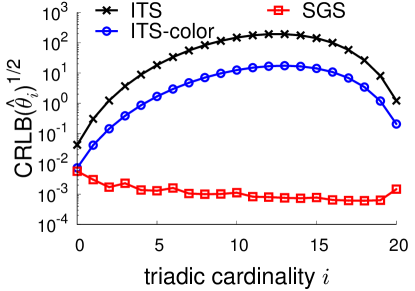
((f)) comparisons

Figure 8: CRLB analysis when graph size is known. $\alpha=0.1$. In LABEL:sub@f:crlb_cmp_1 and LABEL:sub@f:crlb_cmp_2, $p_{\triangle}^{\text{ITS}}=0.1$ and $p_{\triangle}^{\text{ITS-color}}=0.22$. In LABEL:sub@f:crlb_cmp_1, $p_{n}=0.024$. In LABEL:sub@f:crlb_cmp_2, $p_{n}=0.07$.

HepTh	DBLP

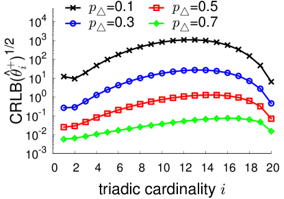
((a)) ITS (ITS-color)

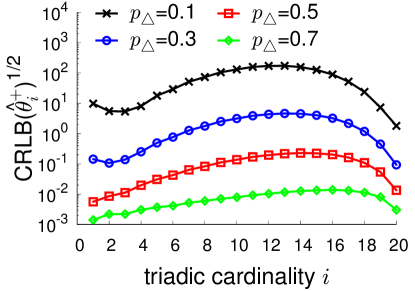
((b)) ITS (ITS-color)

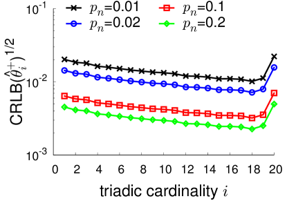
((c)) SGS

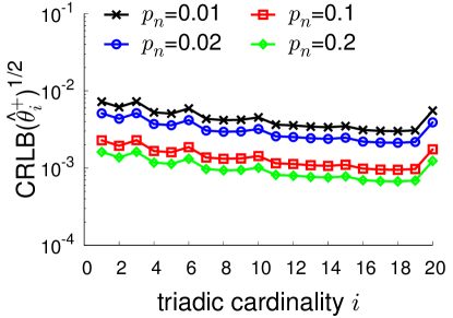
((d)) SGS

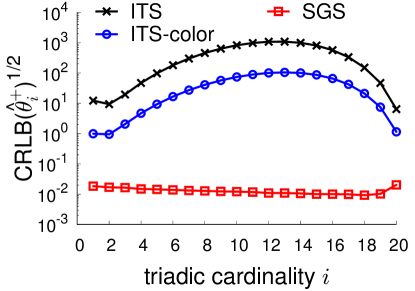
((e)) comparisons

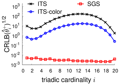
((f)) comparisons

Figure 9: CRLB analysis when graph size is unknown. In ITS and ITS-color, $\alpha=0.1$. Parameters in LABEL:sub@f:crlb_un_cmp_1 and LABEL:sub@f:crlb_un_cmp_2 are the same as in Fig. 8.

VI-B3 NRMSE analysis

CRLB reflects the asymptotic variance of a MLE, i.e., the variance when sample size approaches infinity. However, in practice, we cannot collect infinite many samples because the number of edges in a stream is finite, or afford to use large sample rate. When sample rate is small, or collected edge samples are not large, MLE is usually biased and we cannot leverage CRLB to analyze its performance (see [33, p. 147] for details). Instead, we propose to use the normalized rooted mean squared error (NRMSE) of an estimator, which is defined by $\text{NRMSE}(\hat{\theta}_{i})=\sqrt{\mathbb{E}{(\hat{\theta}_{i}-\theta_{i})^{2}}}/\theta_{i}$. The smaller the NRMSE, the more accurate an estimator is. In the following experiment, we mainly use the HepTh network, and compare different sampling methods using approximately the same amount of edge samples.

We depict the results when graph size is known in Fig. 10. In LABEL:sub@f:nrmse_sm_1 and LABEL:sub@f:nrmse_sm_2, we compare the estimates and NRMSE of different methods. In general, SGS is better than ITS-color, and ITS-color is better than ITS. This observation is consistent with our previous CRLB analysis. The NRMSE plots in LABEL:sub@f:nrmse_sm_2 provide more valuable observations. We observe that SGS can provide more accurate estimates for nodes with small triadic cardinalities than ITS and ITS-color; however, SGS performs much worse than ITS and ITS-color for nodes with large triadic cardinalities. This observation can be explained from the different nature between SGS and ITS based methods. The ITS based methods sample each triangle with identical probability, and if dependence between triangles is negligible, the sampling will be strongly biased towards nodes with many triangles. That is, nodes with larger triadic cardinalities are more likely to be sampled, and for nodes with small triadic cardinalities, the triangles these nodes belonging to will be seldom sampled. This results in that triangles of small triadic cardinality nodes are difficult to be sampled, and hence incurs large estimation error for these nodes. SGS is completely different, and it reserves all the triangles of each node sample. Because nodes are sampled with same probability, node samples will be dominated by nodes with small triadic cardinalities. Hence, SGS can provide more accurate estimates for the head of triadic cardinality distribution. However, SGS is inefficient in sampling nodes with large triadic cardinalities, resulting in large NRMSE at the tail of the triadic cardinality distribution. To address their weaknesses, one way is to increase sampling rates, as depicted in LABEL:sub@f:nrmse_bg_1 and LABEL:sub@f:nrmse_bg_2. We observe that after increasing sampling rates, estimation accuracy increases more or less for each method. An alternative way is to design a mixture estimator, which combines the advantage (and the disadvantage) of each method. For example, we define

$$\hat{\theta}_{i}^{\text{mix}}\triangleq c\hat{\theta}_{i}^{\text{ITS-color}}+(1-c)\hat{\theta}_{i}^{SGS},$$

where $c\in[0,1]$ is a constant. $\hat{\theta}_{i}^{\text{mix}}$ has the property that, its variance is smaller than $\hat{\theta}^{\text{SGS}}$ for nodes with large triadic cardinalities, with the loss of accuracy for nodes with small triadic cardinalities, and the variance of the mixture estimator achieves minimal at $c^{*}=var(\hat{\theta}_{i}^{SGS})/[var(\hat{\theta}_{i}^{\text{ITS-color}})+var(\hat{\theta}_{i}^{SGS})]$. Figs. LABEL:sub@f:nrmse_mx_1 and LABEL:sub@f:nrmse_mx_2 show the results of a mixture estimator with $c=0.5$. We indeed observe improvements for nodes with large triadic cardinalities.

estimates	NRMSE

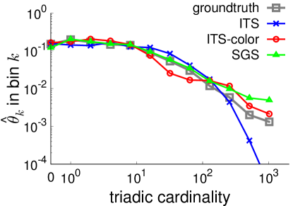
((a)) $p=0.1,p_{n}=0.005$

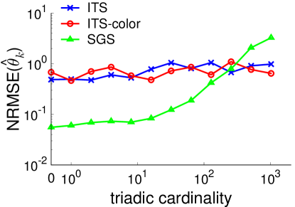
((b)) $p=0.1,p_{n}=0.005$

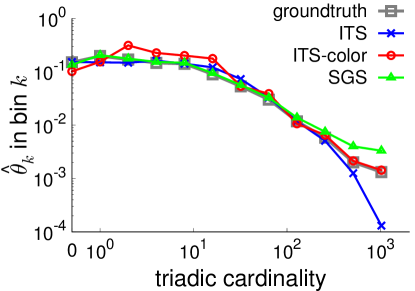
((c)) $p=0.2,p_{n}=0.01$

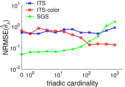
((d)) $p=0.2,p_{n}=0.01$

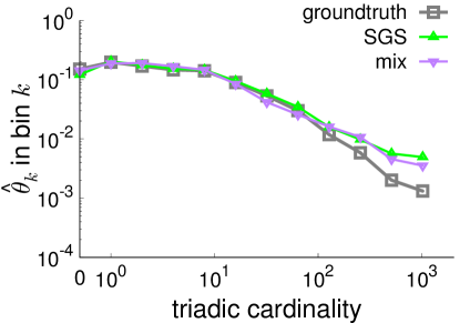
((e)) $p=0.1,p_{n}=0.005,c=0.5$

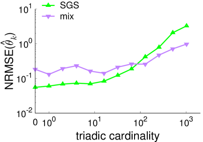
((f)) $p=0.1,p_{n}=0.005,c=0.5$

Figure 10: Estimation accuracy analysis on HepTh when graph size is known.

estimates	NRMSE

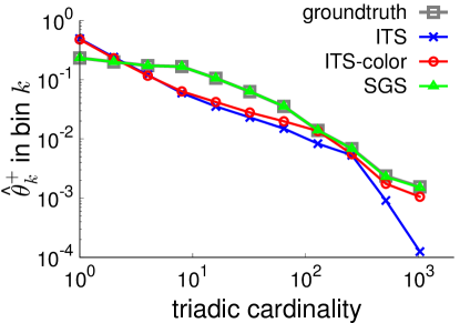
((a)) $p=0.1,p_{n}=0.005$

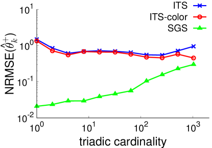
((b)) $p=0.1,p_{n}=0.005$

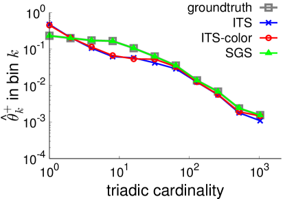
((c)) $p=0.2,p_{n}=0.01$

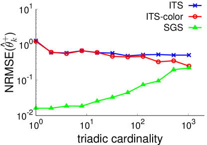
((d)) $p=0.2,p_{n}=0.01$

Figure 11: Estimation accuracy analysis on HepTh when graph size is unknown.

We also conduct experiments when graph size is unknown, and show the results in Fig. 11. The observations are consistent with the results when graph size is known in general, and we observe that SGS has smaller NRMSE than ITS based methods even for nodes with large triadic cardinalities.

Finally, we also conducted experiments on two larger networks, YouTube and Pokec. Here, we mainly compare the computational efficiency of our sampling approach against a naive method that uses all of the original graph to calculate $\theta$ in an exact fashion. The results are depicted in Fig. 12. In general, for ITS, using edge sampling rates between $0.1$ and $0.3$, we have speedup about $10$ to $50$.

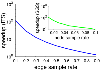
((a)) YouTube

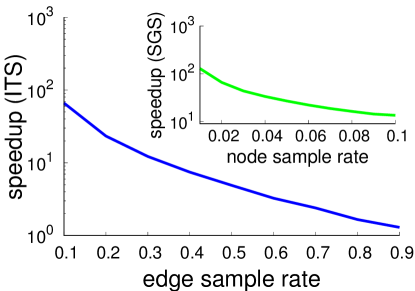
((b)) Pokec

Figure 12: Computational efficiency comparison

VI-C Application: Tracking Triadic Cardinality Distributions during the 2014 Hong Kong Occupy Central Movement

Last, we conduct an application to illustratively show the usefulness of tracking triadic cardinality distributions during the 2014 Hong Kong Occupy Central movement in Twitter.

Hong Kong Occupy Central movement a.k.a. the Umbrella Revolution, began in Sept 2014 when activists in Hong Kong protested against the government and occupied several major streets of Hong Kong to go against a decision made by China’s Standing Committee of the National People’s Congress on the proposed electoral reform. Protesters began gathering from Sept 28 on and we collected the data between Sept 1 and Nov 30 in 2014.

Building a Twitter social activity stream. The input of our solution is a social activity stream from Twitter. For Twitter itself, this stream is easily obtained by directly aggregating tweets of users. While for third parties who do not own user’s tweets, the stream can be obtained by following a set of users, and aggregating tweets from these users to form a social activity stream. Since the movement had already begun prior to our starting this work, we rebuilt the social activity stream by searching tweets containing at least one of the following hashtags: #OccupyCentral, #OccupyHK, #UmbrellaRevolution, #UmbrellaMovement and #UMHK, between Sept 1 and Nov 30 using Twitter search APIs. This produced $66,589$ Twitter users, and these users form the detectors from whom we want to detect bursts. Next, we collect each user’s tweets between Sept 1 and Nov 30, and extract user mentions (i.e., user-user interactions) and user hashtags (i.e., user-content interactions) from tweets to form a social activity stream, with a time span of $91$ days.

Settings. We set the length of a time window to be one day. For interaction bursts caused by user-user interactions, because we know the user population, i.e., $n=66,589$, we apply the first estimation method to obtain $\hat{\theta}=(\hat{\theta}_{0},\ldots,\hat{\theta}_{W})$ for each window. For cascading bursts caused by user-content interactions, as we do not know the number of hashtags in advance, we apply the second method to obtain estimates $\hat{n}_{+}$, i.e., the number of hashtags with at least one influence triangle, and $\hat{\vartheta}^{+}=(\hat{\vartheta}_{1}^{+},\ldots,\hat{\vartheta}_{W}^{+})$ for each window. Combining $\hat{n}_{+}$ with $\hat{\vartheta}^{+}$, we use $\hat{n}_{+}\hat{\vartheta}^{+}$, i.e., frequencies, to characterize patterns of user-content interactions in each window.

Results. We first answer the question: are there significant differences for the two distributions before and during the movement? In Fig. 13, we compare the distributions before (Sept 1 to Sept 3) and during (Sept 28 to Sept 30) the movement. We can find that when the movement began on Sept 28, the distributions of the two kinds of interactions shift to the right, indicating that many interaction and influence triangles form when the movement starts. Therefore, these observations confirm our motivation for detecting bursts by tracking triadic cardinality distributions.

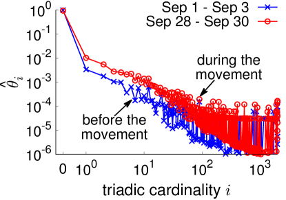
((a)) Interaction burst

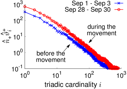
((b)) Cascading burst

Figure 13: Triadic cardinality distributions before and during the movement. Estimated using a mixture estimator with $c=0.5,p=0.2,p_{n}=0.002$.

Next, we track the daily triadic cardinality distributions to look up the distribution change during the movement. To characterize the sudden change in the distributions, we use KL divergence to calculate the difference between $\hat{\theta}$ and a base distribution $\theta_{\text{base}}$. The base distribution $\theta_{\text{base}}$ represents a distribution when the network is dormant, i.e., no bursts are occurring. Here we omit the technique details, and simply average the triadic cardinality distributions from Sept 1 to Sept 7 to obtain an approximate base distribution $\hat{\theta}_{\text{base}}$, and show the KL divergence $D_{\text{KL}}(\hat{\theta}_{\text{base}}\parallel\hat{\theta})$ in Fig. 14.

Figure 14: Triadic cardinality distributions change during the 2014 Hong Kong Occupy Central movement in Twitter.

We find that the KL divergence exhibits a sudden increase on Sept 28 when the movement broke out. The movement keeps going on and reaches a peak on Oct 19 when repeated clashes happened in Mong Kok at that time. The movement temporally returned to peace between Oct 22 and Oct 25, and restarted again after Oct 26. In Fig. 14, we also show the estimated number of hashtags having at least one influence triangle. Its trend is similar to the trend of KL divergence which indicates that the movement is accompanied with rumors spreading in a word-of-mouth manner.

In conclusion, the application in this section demonstrates that the using of the triadic cardinality distribution can track bursts from a social activity stream and the result is consistent with real world events.

VII Related Work

Kleinberg first studied the topic of burst detection from streams in [10], where he used a multistate automaton to model a stream consisting of messages, e.g., an email stream. The occurrence of a burst is modeled by an underlying state transiting into a bursty state that emits messages at a higher rate than at the non-bursty state. Based on this model, many variant models are proposed for detecting bursts from document streams [11, 38], e-commerce queries [12], time series [39], and social networks [13]. Although these models are theoretically interesting, some assumptions made by them are inappropriate, such as the Poisson process of message arrivals (see [40]) and nonexistence of spams/bots, which may limit their practical usage.

The topic of (anomaly) event detection is also related to our work. Recently, Chierichetti et al. [41] found that Twitter user tweeting and retweeting count information can be used to detect sub-events during some large event such as the soccer World Cup of 2010. Takahashi et al. [42] proposed a probabilistic model to detect emerging topics in Twitter by assigning an anomaly score for each user. Sakaki et al. [43] proposed a spatiotemporal model to detect earthquakes using tweets. Manzoor et al. [44] studied anomaly event detection from a graph stream based on graph similarity metrics. Different from theirs, we exploit the triangle structure existing in user interactions which is robust against common spams and can be efficiently estimated using our method.

The triangle structure can be considered as a type of network motif, which is introduced in [45] when the authors were studying how to characterize structures of different types of networks. Turkett et al. [46] used motifs to analyze computer network usage, and [47] proposed sampling methods to efficiently estimate motif statistics in a large graph. However, both the motivation in [46] and subgraph statistics defined in [47] are different from ours.

Recently, there are many works on estimating the number of global and local triangles [22, 48, 49, 50, 21, 51, 52, 53], or clustering coefficient [54] in a large graph. However, triadic cardinality distribution is much complicated than triangle counts, and these methods cannot be used to estimate the triadic cardinality distribution. Becchetti et al. [55] used a min-wise hashing method to approximately count triangles for each individual node in an undirected simple graph. Our method does not rely on counting triangles for each individual node. Rather, we use a carefully designed estimator to estimate the statistics from a sampled graph, which is demonstrated to be efficient and accurate.

VIII Conclusion

Online social networks provide various ways for users to interact with other users or media content over the Internet, which bridge the online and offline worlds tightly. This provides an opportunity to researchers to leverage online users’ interactions to detect bursts that may cause negative impacts to the offline world. This work studied the burst detection problem from a high-speed social activity stream generated by user’s interactions in an OSN. We show that the emergence of bursts caused by either user-user or user-content interaction are accompanied with the formation of triangles in users’ interaction networks. This finding prompts us to devise a novel method for burst detection in OSNs by introducing the triadic cardinality distribution. Triadic cardinality distribution is found to be robust against common spamming attacks which makes it a more suitable indicator for detecting bursts than the volume of user activities. We design a sample-estimate solution that aims to estimate triadic cardinality distribution from a sampled social activity stream. We show that, in general, SGS is more efficient in gathering information from data than ITS based methods. However, SGS incurs larger NRMSE than ITS for nodes with large triadic cardinalities. We can combine ITS and SGS and use a mixture estimator to further reduce the NRMSE of SGS at the tail estimates. We believe our work sets the foundation for robust burst detection, and it is an open problem for finding and designing better or optimal sampling and estimation methods.

References

- [1] M. Harvey, “Fans mourn artist for whom it didn’t matter if you were black or white,” http://wayback.archive.org/web/20100531165925/http://www.timesonline.co.uk/tol/news/world/us_and_americas/article6580897.ece, Retrived Jun 2017.
- [2] M. Shiels, “Web slows after Jackson’s death,” http://news.bbc.co.uk/2/hi/technology/8120324.stm, Retrived Jun 2017.
- [3] “London riots: More than 2,000 people arrested over disorder,” http://www.mirror.co.uk/news/uk-news/london-riots-more-than-2000-people-185548, Retrived Jun 2017.
- [4] Z. Chu, S. Gianvecchio, H. Wang, and S. Jajodia, “Who is tweeting on Twitter: Human, bot, or cyborg?” in Proceedings of the 26th Annual Computer Security Applications Conference, 2010.
- [5] C. Grier, K. Thomas, V. Paxson, and M. Zhang, “@spam: The underground on 140 characters or less,” in Proceedings of the ACM SIGSAC Conference on Computer and Communications Security, 2010.
- [6] G. Stringhini, C. Kruegel, and G. Vigna, “Detecting spammers on social networks,” in Proceedings of the 26th Annual Computer Security Applications Conference, 2010.
- [7] Y. Boshmaf, I. Muslukhov, K. Beznosov, and M. Ripeanu, “The socialbot network: When bots socialize for fame and money,” in Proceedings of the 27th Annual Computer Security Applications Conference, 2011.
- [8] K. Thomas, C. Grier, V. Paxson, and D. Song, “Suspended accounts in retrospect: An analysis of Twitter spam,” in Proceedings of the 11th ACM SIGCOMM Conference on Internet Measurement, 2011.
- [9] A. Beutel, W. Xu, V. Guruswami, C. Palow, and C. Faloutsos, “CopyCatch: Stopping group attacks by spotting lockstep behavior in social networks,” in Proceedings of the 22nd International World Wide Web Conference, 2013.
- [10] J. Kleinberg, “Bursty and hierarchical structure in streams,” in Proceedings of the 8th ACM SIGKDD International Conference on Knowledge Discovery and Data Mining, 2002.
- [11] J. Yi, “Detecting buzz from time-sequenced document streams,” in Proceedings of the IEEE International Conference on e-Technology, e-Commerce and e-Service, 2005.
- [12] N. Parikh and N. Sundaresan, “Scalable and near real-time burst detection from ecommerce queries,” in Proceedings of the 14th ACM SIGKDD International Conference on Knowledge Discovery and Data Mining, 2008.
- [13] M. Eftekhar, N. Koudas, and Y. Ganjali, “Bursty subgraphs in social networks,” in Proceedings of the 6th International ACM Conference on Web Search and Data Mining, 2013.
- [14] D. J. Watts and S. H. Strogatz, “Collective dynamics of ‘small-world’ networks,” Nature, vol. 393, pp. 440–442, 1998.
- [15] G. Kossinets and D. J. Watts, “Empirical analysis of an evolving social network,” Science, vol. 311, no. 5757, pp. 88–90, 2006.
- [16] J. Leskovec, M. McGlohon, C. Faloutsos, N. Glance, and M. Hurst, “Cascading behavior in large blog graphs,” in Proceedings of the 7th SIAM International Conference on Data Mining, 2007.
- [17] T. Rodrigues, F. Benevenuto, M. Cha, K. P. Gummadi, and V. Almeida, “On word-of-mouth based discovery of the web,” in Proceedings of the 11th ACM SIGCOMM Conference on Internet Measurement, 2011.
- [18] A. Tsotsis, “First credible reports of Bin Laden’s death spread like wildfire on Twitter,” https://techcrunch.com/2011/05/01/news-of-osama-bin-ladens-death-spreads-like-wildfire-on-twitter, Retrived Jun 2017.
- [19] R. Krikorian, “New tweets per second record, and how!” https://blog.twitter.com/engineering/en_us/a/2013/new-tweets-per-second-record-and-how.html, Retrived Jun 2017.
- [20] R. Pagh and C. E. Tsourakakis, “Colorful triangle counting and a MapReduce implementation,” Journal of Information Processing Letters, vol. 112, no. 7, pp. 277–281, 2012.
- [21] N. K. Ahmed, N. Duffield, J. Neville, and R. Kompella, “Graph sample and hold: A framework for big-graph analytics,” in Proceedings of the 20th ACM SIGKDD International Conference on Knowledge Discovery and Data Mining, 2014.
- [22] C. E. Tsourakakis, U. Kang, G. L. Miller, and C. Faloutsos, “DOULION: Counting triangles in massive graphs with a coin,” in Proceedings of the 15th ACM SIGKDD International Conference on Knowledge Discovery and Data Mining, 2009.
- [23] M. Gjoka, M. Kurant, C. T. Butts, and A. Markopoulou, “Practical recommendations on crawling online social networks,” IEEE Journal on Selected Areas in Communications, vol. 29, no. 9, pp. 1872–1892, 2011.
- [24] N. Duffield, C. Lund, and M. Thorup, “Estimating flow distributions from sampled flow statistics,” in Proceedings of the ACM Special Interest Group on Data Communication, 2003.
- [25] B. Ribeiro, D. Towsley, T. Ye, and J. C. Bolot, “Fisher information of sampled packets: An application to flow size estimation,” in Proceedings of the 6th ACM SIGCOMM Conference on Internet Measurement, 2006.
- [26] P. Tune and D. Veitch, “Fisher information in flow size distribution estimation,” IEEE Transactions on Information Theory, vol. 57, no. 10, pp. 7011–7035, 2011.
- [27] P. Wang, X. Guan, J. Zhao, J. Tao, and T. Qin, “A new sketch method for measuring host connection degree distribution,” IEEE Transactions on Information Forensics and Security, vol. 9, no. 6, pp. 948–960, 2014.
- [28] D. Veitch and P. Tune, “Optimal skampling for the flow size distribution,” IEEE Transactions on Information Theory, vol. 61, no. 6, pp. 3075–3099, 2015.
- [29] “Beta-binomial distribution,” https://en.wikipedia.org/wiki/Beta-binomial_distribution, Retrived Jun 2017.
- [30] C. Yu and D. Zelterman, “Sums of dependent Bernoulli random variables and disease clustering,” Statistics and Probability Letters, vol. 57, no. 1, pp. 363–373, 2002.
- [31] M. Durand and P. Flajolet, “Loglog counting of large cardinalities,” in Proceedings of the 11th Annual European Symposium on Algorithms, 2003.
- [32] J. Zhao, J. C. Lui, D. Towsley, P. Wang, and X. Guan, “Tracking triadic cardinality distributions for burst detection in social activity streams,” in ACM Conferencec on Online Social Networks, 2015.
- [33] H. L. V. Trees, Detection, Estimation, and Modulation Theory, Part I. Wiley-Interscience, 2001.
- [34] “Cramér-Rao bound,” https://en.wikipedia.org/wiki/Cram%C3%A9r%E2%80%93Rao_bound#Multivariate_case, Retrived Aug 2017.
- [35] J. D. Gorman and A. O. Hero, “Lower bounds for parametric estimation with constraints,” IEEE Transition on Information Theory, vol. 26, no. 6, pp. 1285–1301, 1990.
- [36] B. Klimt and Y. Yang, “The Enron corpus: A new dataset for email classification research,” in Proceeding of the European Conference on Machine Learning and Principles and Practice of Knowledge Discovery in Databases, 2004.
- [37] L. Backstrom, E. Bakshy, J. Kleinberg, T. M. Lento, and I. Rosenn, “Center of attention: How Facebook users allocate attention across friends,” in Proceedings of the 5th International AAAI Conference on Weblogs and Social Media, 2011.
- [38] M. Mathioudakis, N. Bansal, and N. Koudas, “Identifying, attributing and describing spatial bursts,” in Proceedings of the VLDB Endowment, 2010.
- [39] Y. Zhu and D. Shasha, “Efficient elastic burst detection in data streams,” in Proceedings of the 9th ACM SIGKDD International Conference on Knowledge Discovery and Data Mining, 2003.
- [40] A.-L. Barabasi, “The origin of bursts and heavy tails in human dynamics,” Nature, vol. 435, pp. 207–211, 2005.
- [41] F. Chierichetti, J. Kleinberg, R. Kumar, M. Mahdian, and S. Pandey, “Event detection via communication pattern analysis,” in Proceedings of the 8th International AAAI Conference on Weblogs and Social Media, 2014.
- [42] T. Takahashi, R. Tomioka, and K. Yamanishi, “Discovering emerging topics in social streams via link anomaly detection,” in Proceedings of the IEEE International Conference on Data Mining, 2011.
- [43] T. Sakaki, M. Okazaki, and Y. Matsuo, “Earthquake shakes Twitter users: Real-time event detection by social sensors,” in Proceedings of the 19th International World Wide Web Conference, 2010.
- [44] E. Manzoor, S. M. Milajerdi, and L. Akoglu, “Fast memory-efficient anomaly detection in streaming heterogeneous graphs,” in KDD, San Francisco, California, USA, 2016.
- [45] R. Milo, S. Shen-Orr, S. Itzkovitz, N. Kashtan, D. Chklovskii, and U. Alon, “Network motifs: Simple building blocks of complex networks,” Science, vol. 298, no. 5594, pp. 824–827, 2002.
- [46] W. Turkett, E. Fulp, C. Lever, and J. Edward Allan, “Graph mining of motif profiles for computer network activity inference,” in Proceedings of the 7th Workshop on Mining and Learning with Graphs, 2011.
- [47] P. Wang, J. C. Lui, B. Ribeiro, D. Towsley, J. Zhao, and X. Guan, “Efficiently estimating motif statistics of large networks,” ACM Transactions on Knowledge Discovery from Data, vol. 9, no. 2, pp. 1–27, 2014.
- [48] C. Budak, D. Agrawal, and A. E. Abbadi, “Structural trend analysis for online social networks,” in Proceedings of the VLDB Endowment, 2011.
- [49] A. Pavan, K. Tangwongsan, S. Tirthapura, and K.-L. Wu, “Counting and sampling triangles from a graph stream,” in Proceedings of the VLDB Endowment, 2013.
- [50] M. Jha, C. Seshadhri, and A. Pinar, “A space efficient streaming algorithm for triangle counting using the birthday paradox,” in Proceedings of the 19th ACM SIGKDD International Conference on Knowledge Discovery and Data Mining, 2013.
- [51] Y. Lim and U. Kang, “MASCOT: Memory-efficient and accurate sampling for counting local triangles in graph streams,” in Proceedings of the 21st ACM SIGKDD International Conference on Knowledge Discovery and Data Mining, Sydney, Australia, 2015.
- [52] L. D. Stefani, A. Epasto, M. Riondato, and E. Upfal, “TRIEST: Counting local and global triangles in fully-dynamic streams with fixed memory size,” in Proceedings of the 22nd ACM SIGKDD International Conference on Knowledge Discovery and Data Mining, 2016.
- [53] B. Wu, K. Yi, and Z. Li, “Counting triangles in large graphs by random sampling,” IEEE Transactions on Knowledge and Data Engineering, vol. 28, no. 8, pp. 2013–2026, 2016.
- [54] C. Seshadhri, A. Pinar, and T. G. Kolda, “Triadic measures on graphs: The power of wedge sampling,” in Proceedings of the 13th SIAM International Conference on Data Mining, 2013.
- [55] L. Becchetti, P. Boldi, C. Castillo, and A. Gionis, “Efficient semi-streaming algorithms for local triangle counting in massive graphs,” in Proceedings of the 14th ACM SIGKDD International Conference on Knowledge Discovery and Data Mining, 2008.