Sampling Online Social Networks by
Random Walk with Indirect Jumps

Abstract

Random walk-based sampling methods are gaining popularity and importance in characterizing large networks. While powerful, they suffer from the slow mixing problem when the graph is loosely connected, which results in poor estimation accuracy. Random walk with jumps (RWwJ) can address the slow mixing problem but it is inapplicable if the graph does not support uniform vertex sampling (UNI). In this work, we develop methods that can efficiently sample a graph without the necessity of UNI but still enjoy the similar benefits as RWwJ. We observe that many graphs under study, called target graphs, do not exist in isolation. In many situations, a target graph is related to an auxiliary graph and a bipartite graph, and they together form a better connected two-layered network structure. This new viewpoint brings extra benefits to graph sampling: if directly sampling a target graph is difficult, we can sample it indirectly with the assistance of the other two graphs. We propose a series of new graph sampling techniques by exploiting such a two-layered network structure to estimate target graph characteristics. Experiments conducted on both synthetic and real-world networks demonstrate the effectiveness and usefulness of these new techniques.

1 Introduction

Online social networks (OSNs) such as Facebook and Twitter have attracted much attention in recent years because of their ever-increasing popularity and importance in our daily lives. An OSN not only provides a platform for people to connect with their friends, but also offers an opportunity to study various user characteristics, which are valuable in many applications such as understanding human behaviors [1, 2, 3] and inferring user preferences [4, 5]. Exactly measuring user characteristics requires the complete OSN data. For third parties who do not possess the data, they can only rely on public APIs to crawl the OSN. However, commercial OSNs are typically unwilling to grant third parties full permission to access the data due to user privacy and business secrecy. They often impose barriers to limit third parties’ large-scale crawling [6], e.g., by limiting the API requesting rate [7, 8]. As a result, collecting the complete data of a large-scale OSN is practically impossible.

To address this challenge, sampling methods have been developed, i.e., a small fraction of OSN users are sampled and used to estimate the OSN user characteristics. In the literature, random walk based sampling methods have gained popularity [9, 10, 11, 12, 13, 14, 15]. In a typical random walk sampling, a walker is launched over a graph, which continuously moves from a node to one of its neighbors selected uniformly at random, to obtain a collection of node samples. These samples can be used to obtain unbiased estimates of nodal or topological properties of the graph. Because a random walk only explores neighborhood of a node during sampling, it is suitable for crawling and sampling large-scale OSNs.

1.1 Problems in Random Walk Based Sampling

While random walk sampling is powerful, if a graph is loosely connected, e.g., consists of communities, it will suffer from slow mixing [16], i.e., requires a long “burn-in” period to reach steady state, which results in the need of a large number of samples in order to achieve desired estimation accuracy. Previous studies have found that mixing times in many real-world networks are larger than expected [17].

To overcome the slow mixing problem, an effective approach is to incorporate uniform node sampling (UNI) into random walk sampling, and enable the walker to jump to other parts of the graph while walking, aka the random walk with jumps (RWwJ) [10, 13, 15]. In UNI, a node is independently sampled uniformly at random from the graph, and in practice, if users in an OSN have unique numerical IDs, then UNI is conducted by generating random numbers in the ID space and including those valid IDs as UNI samples. RWwJ then leverages UNI to perform jumps on a graph. Specifically, at each step of RWwJ, the walker jumps with a probability determined by the node where it currently resides, to a node sampled by UNI. By incorporating UNI into random walk sampling, the walker can jump out of a community or disconnected component of a graph, and avoid being trapped, thereby reducing the mixing time [10].

The main problem of using RWwJ to sample an OSN is that, some OSNs may not support UNI at all because user IDs are not numerical, or the UNI is resource intensive because the valid IDs are sparsely populated. For example, in Pinterest [18], a user’s ID is an arbitrary length string, which hence makes UNI practically impossible. In MySpace and Flickr, although the user IDs are numerical, the fractions of valid user IDs are only about $10\%$ and $1.3\%$, respectively [13]; in other words, one has to generate about $10$ (or $77$) random numbers (and verify them by querying OSN APIs) to obtain one valid user ID in MySpace (or Flickr). In some situations, the valid ID space could become extremely sparse.

Example 1 (Sampling Weibo users in a city).

Suppose we want to measure user characteristics in Sina Weibo [19], which is a popular OSN in China. Rather than measuring all the Weibo users, we are only interested in users who checked in venues in a specified city. For example, users who shared check-in information at tourist spots, hotels, and restaurants of a city could be used to evaluate the city’s internationality, economic index, etc. Suppose the users who checked in the city account for about $0.1\%$ of all Weibo users. We also know that each Weibo user has a unique $10$-digit numerical ID, and the fraction of valid IDs is about $10\%$.

In the above example, when conducting UNI, we expect that a randomly generated number is a valid user ID, and the corresponding user checked in the city. This happens with probability $10^{-4}$, and as a result, we have to try $10^{4}$ times on average to obtain one valid UNI sample! Without the efficiency of conducting UNI on a graph, we cannot perform jumps, and hence RWwJ is inapplicable. This raises the following problem we want to solve in this work:

If we cannot perform jumps on a graph, can we conduct random walk sampling that still has the similar benefits as RWwJ?

1.2 Overview of Our Approach

In this work, we design a series of graph sampling techniques that can efficiently sample a network without the necessity of UNI, but still enjoy the similar benefits as RWwJ. The main idea behind our method is to leverage a “two-layered network structure” to perform “indirect jumps” on the graph under study, and indirect jumps can bring similar benefits as the direct jumps in RWwJ. We first use Example 1 to briefly explain what we mean by two-layered network structure, and then this discovery immediately motivates us to design an indirect sampling method, which enables us to perform indirect jumps on a graph.

In Example 1, directly applying UNI on the user network is inefficient because of the sparsity of user ID space, i.e., a randomly generated number is very likely to be an invalid user ID, or the user just lies outside of the city. Since directly sampling users by UNI is difficult, we propose to sample users in an indirect manner. We notice that besides the user network, we are actually also provided with a space consisting of venues on a map, as illustrated in Fig. 1(a). If we can sample venues in the city by UNI (or its variants), then we can sample users indirectly because venues and users are related by their check-in relationships. The check-ins tell us which user checked in which place, and for a given venue, we can query the users who checked in this venue, and hence easily obtain a user sample from a venue sample. Sampling venues in an area is indeed possible by leveraging the APIs provided by many location-based OSNs (LBSNs). Many LBSNs provide APIs for querying venues within an area specified by a rectangle region with southwest and northeast corners latitude-longitude coordinates given [21, 22]. This function can be used to design efficient sampling methods for sampling venues in an area on a map [23, 24, 25]. For example, we can efficiently sample a venue in the city specified by a rectangle region, and the probability of obtaining this venue sample is calculable. Note that a user sample obtained from a venue sample is no longer uniformly distributed. Because if a user checked in many venues in the city, the user is likely to be heavily sampled. But such bias can be easily removed by a reweighting strategy, which we will elaborate in Section 4.

((a)) user network and venues on a map

((b)) accounts sharing between two OSNs

((c)) item network and tag/category network

Figure 1: Examples of two-layered network structures

An important lesson learned from solving the problem in Example 1 is that, the two-layered network structure, consisting of the user network layer and the venues layer, can help us to obtain samples of one layer when sampling another layer is easy. Hence, this enables us to conduct “indirect jumps” on the user network with the help of venue sampling. We further find that the two-layered network structure is not unique to the problem in Example 1, but is pervasive in a wide range of graph sampling problems, and more examples will be presented in Section 3. Hence, it is necessary to develop some unified graph sampling techniques that can leverage the two-layered network structure to address these graph sampling problems.

In general, there are three graphs related to the two-layered network structure: (1) a target graph, whose characteristics are of interest to us and need to be estimated, e.g., the user sub-network in Example 1; (2) an auxiliary graph, which is easier to be sampled than the target graph, e.g., the venues can be thought of as nodes in an auxiliary graph, and Example 1 is a special case where the auxiliary graph has an empty edge set; and (3) a bipartite graph that connects nodes in the target and auxiliary graphs. When directly sampling the target graph is difficult, we can turn to sample the auxiliary graph, and the bipartite graph bridges the two sample spaces and allows us to sample the target graph in an indirect manner. This thus enables us to perform indirect jumps on the target graph, and allows us to develop random walk sampling methods with indirect jumps that have the similar benefits as RWwJ.

1.3 Contributions

We make three contributions in this work:

• We discover the pervasiveness and usefulness of a “two-layered network structure”, that exists in many real-world applications, and can be exploited to efficiently sample a graph in an indirect manner if directly sampling the graph is difficult.

• We design three new sampling techniques by leveraging such a two-layered network structure. These new techniques enable us to conduct random walk sampling that has the similar benefits as RWwJ.

• We conduct extensive experiments on both synthetic and real-world networks to validate our proposed methods. The experimental results demonstrate the effectiveness of our designed sampling techniques.

1.4 Outline

The reminder of this paper will proceed as follows. In Section 2, we provide some preliminaries about graph sampling. In Section 3, we formally define the two-layered network structure along with more examples. In Section 4 we elaborate three new sampling methods. In Section 5, we conduct experiments to validate our methods. Section 6 reviews some related literature, and Section 7 concludes.

2 Preliminaries

In this section, we provide some preliminaries about the graph sampling problem, and review a random walk based sampling method named random walk with jumps (RWwJ).

2.1 Graph Sampling

An OSN can be modeled as an undirected graph $G=(U,E)$, where $U$ is a finite set of nodes representing users, and $E\in U\times U$ is a set of edges representing relations between users. We assume that the graph $G$ has no self-loops and no multiple edges connecting two nodes. Also, the graph size $|U|=n$ may be not known in advance.

Let $f\colon U\mapsto\mathbb{R}$ be any desired characteristic function that maps a node in the graph to a real number. The goal of measuring the characteristic of graph $G$ is to estimate

$$\theta\triangleq\frac{1}{n}\sum_{u\in U}f(u),$$

which is the aggregated nodal characteristic of the graph. For example, in an OSN, we let $f(u)=1$ if user $u$ is female, and otherwise $f(u)=0$, then $\theta$ represents the fraction of female users in the OSN.

The goal of graph sampling is to design an algorithm for collecting node samples $S$ from graph $G$, constrained by a budget $|S|\leq B\ll n$, and for providing unbiased estimate of $\theta$ with low statistical error.

2.2 Random Walk with Jumps

Random walk with jumps (RWwJ) [10] is a popular graph sampling method that can address the slow mixing issue of a simple random walk when the graph has community structures. RWwJ generally works as follows: A walker starts from a node in the graph, and at each step, it moves to a neighbor selected uniformly at random, or jumps to a node uniformly sampled from the graph, and the probability of jumping is determined by the node where the walker currently resides; this process continues until enough samples are collected.

An easier way to think about RWwJ is that, we modify the structure of the original graph by connecting every node in the graph to a virtual jumper node, with edge weight $\alpha\geq 0$; then a simple random walk on this modified graph is equivalent to RWwJ. Figure 2 illustrates RWwJ on a loosely connected graph. Comparing the modified graph with the original graph, we can find that the modified graph always has larger graph conductance than the original graph, and because larger graph conductance usually implies faster mixing of a random walk [16], hence, RWwJ has the advantage of faster mixing than a simple random walk on poorly connected graphs [10].

Figure 2: RWwJ is viewed as a simple random walk on the modified graph.

In RWwJ, the probability transition matrix of the underlying Markov chain is given by

$$P_{ij}^{\text{RWwJ}}=\begin{cases}\frac{\alpha/n+1}{d_{i}+\alpha},&(i,j)\in E,\\ \frac{\alpha/n}{d_{i}+\alpha},&(i,j)\notin E.\\ \end{cases}$$

That is, if $(i,j)\in E$, the walker starting from $i$ could walk to $j$ (in one step) through the edge $(i,j)$ with probability $\frac{1}{d_{i}+\alpha}$; or jump to $j$ through UNI with probability $\frac{\alpha}{d_{i}+\alpha}\cdot\frac{1}{n}=\frac{\alpha/n}{d_{i}+\alpha}$; thus the transition probability on edge $(i,j)$ is $\frac{\alpha/n+1}{d_{i}+\alpha}$. If $(i,j)\notin E$, the walk starting from $i$ can only walk to $j$ (in one step) by jumping with probability $\frac{\alpha/n}{d_{i}+\alpha}$.

When RWwJ reaches the steady state, a node $u\in U$ is sampled with probability proportional to $d_{u}+\alpha$. If we let $S$ denote the samples collected by RWwJ, an asymptotically unbiased estimator of $\theta$ is given by

$$\hat{\theta}^{\text{RWwJ}}=\frac{1}{Z^{\text{RWwJ}}}\sum_{s\in S}\frac{f(s)}{d_{s}+\alpha},$$ (1)

where $Z^{\text{RWwJ}}\triangleq\sum_{s\in S}1/(d_{s}+\alpha)$. We can understand the unbiasedness of Estimator (1) by leveraging the ratio form of the Law of Large Numbers of Markov chains.

Lemma 1 (Law of Large Numbers [26, p.427–428]).

Let $S$ be a sample path obtained by a Markov chain defined on state space $U$ with stationary distribution $\pi$. For any function $f,g\colon U\mapsto\mathbb{R}$, and let $F_{S}(f)\triangleq\sum_{s\in S}f(s)$, $\mathbb{E}_{\pi}[f]\triangleq\sum_{u\in U}\pi_{u}f(u)$. It holds that

$$\lim_{|S|\rightarrow\infty}\frac{1}{|S|}F_{S}(f) =\mathbb{E}_{\pi}[f]\quad a.s.,$$ (2)

$$\lim_{|S|\rightarrow\infty}\frac{F_{S}(f)}{F_{S}(g)} =\frac{\mathbb{E}_{\pi}[f]}{\mathbb{E}_{\pi}[g]}\quad a.s..$$ (3)

Here, “a.s.” denotes “almost sure” convergence, i.e., the event of interest happens with probability one.

Therefore, in Estimator (1), replacing $f(s)/(d_{s}+\alpha)$ by $f(s)$, and $1/(d_{s}+\alpha)$ by $g(s)$, we obtain that $\hat{\theta}^{\text{RWwJ}}$ converges to $\mathbb{E}_{\pi}[f]/\mathbb{E}_{\pi}[g]=\theta$, almost surely.

Although RWwJ can address the slow mixing problem, it requires UNI to perform jumps on a graph. If the OSN does not support UNI, or UNI is inefficient, RWwJ becomes inapplicable. In this work, we introduce a two-layered network structure that exists in many real-world applications, and we will show that such a structure can be leveraged to design random walk sampling methods having the similar benefits as RWwJ even though we cannot conduct UNI on the graph.

3 Two-Layered Network Structure

In this section, we first formally describe the two-layered network structure we discovered in Example 1. Then we provide more examples to demonstrate the pervasiveness of such a structure.

3.1 Definition

We use three undirected graphs to describe a two-layered network structure: $G(U,E)$, $G^{\prime}(V,E^{\prime})$, and $G_{b}(U,V,E_{b})$, where $U,V$ are two sets of nodes, and $E\subseteq U\times U,E^{\prime}\subseteq V\times V,E_{b}\subseteq U\times V$ are three sets of edges. More specifically,

• $G(U,E)$ is the target graph, whose characteristic $\theta$ is of interest to us and needs to be measured. For example, the user social network in Example 1 can be treated as the target graph.

• $G^{\prime}(V,E^{\prime})$ is an auxiliary graph, which can be more efficiently sampled than the target graph. In Example 1, we can construct an auxiliary graph where the nodes represent the venues in the city, and the edge set is left empty (i.e., $E^{\prime}=\emptyset$).

• $G_{b}(U,V,E_{b})$ is a bipartite graph that connects nodes in the target and auxiliary graphs. In Example 1, the bipartite graph is formed by users, venues and their check-in relationships.

An example of such a two-layered network structure is illustrated in Fig. 3. The target graph consists of two disconnected components, however, if we view the three graphs as a whole, they form a better connected graph than the target graph itself. Hence, it is possible to sample target graph efficiently with the help of the other two graphs. With this intuition in mind, we will see in next section that we indeed can design efficient sampling methods by leveraging this two-layered network structure.

Figure 3: Illustration of the two-layered network structure.

3.2 More Examples

The two-layered network structure is not unique to Example 1, but exists in a wide range of real-world applications. In the following, we provide more examples.

Example 2 (Accounts sharing between two OSNs).

Many OSNs now support using an existing OSN’s accounts to login another OSN. For example, Facebook users can login Pinterest using their Facebook accounts. This naturally forms a two-layered network structure consisting of Facebook and Pinterest. Suppose we want to measure Pinterest, then we can let target graph represent Pinterest, auxiliary graph represent Facebook, and bipartite graph represent their account sharing relations.

Figure 1(b) illustrates Example 2. Note that Pinterest does not support UNI, hence RWwJ is inapplicable. Instead, using the techniques developed in this work, we will be able to leverage Facebook to sample Pinterest.

Example 3 (Amazon item network and categories).

Items in Amazon are related with each other to form an item network. Each item also belongs to one or more categories. Meanwhile, Amazon provides a complete category list to facilitate customers to quickly navigate to the items they are looking for. This forms a two-layered network structure consisting of items and categories. Suppose we want to measure the item network, then we can let target graph represent the item network, auxiliary graph represent the category list, and bipartite graph represent the affiliation relations between items and categories.

Figure 1(c) illustrates Example 3. Note that categories could also be tags and they may also form a tag network. Items are very likely to form clusters, and hence easily trap a random walker. If we can leverage the category information, and help a random walker to jump out of clusters, we can sample the item network in a more efficient way.

4 Sampling Design

In this section, we leverage the two-layered network structure and design three new sampling techniques to sample and characterize the target graph.

4.1 Indirectly Sampling Target Graph by Vertex Sampling on Auxiliary Graph (VS^A)

The first method assumes that vertex sampling is easier to conduct on the auxiliary graph than on the target graph, as is the case in Example 1. We present a sampling method VS^A (and its two implementations VS^A-I and VS^A-II) to indirectly sample the target graph under this setting. The basic idea of VS^A is illustrated in Fig. 4.

Figure 4: Illustration of VS^A. Edges in $G$ and $G^{\prime}$ are omitted.

VS^A-I. Assume that a node $v\in V$ is sampled with probability $p_{v}\propto a_{v}>0$ in auxiliary graph $G^{\prime}$. For example, if auxiliary graph $G^{\prime}$ supports UNI, then $a_{v}\equiv 1,\forall v\in V$. The simplest way to implement VS^A is as follows: We first sample a node $v\in V$ in $G^{\prime}$, and then sample a neighbor of $v$ in $G_{b}$ uniformly at random, denoted by $u$. Obviously, $u\in U$, and we collect $u$ as a sample. We refer to this simple sampling method as VS^A-I, and will show that samples collected by VS^A-I can indeed yield unbiased estimate of $\theta$. The detailed design of VS^A-I is described as follows.

Sampling design. VS^A-I repeats the following two steps until sample collection $S$ reaches budget $B$.

• Sample a node $v$ from auxiliary graph $G^{\prime}$;

• If $v$ has neighbors in bipartite graph $G_{b}$, sample a neighbor $u$ uniformly at random, and put $u$ into samples $S$.

Estimator. In VS^A-I, we can see that a node $u\in U$ is sampled with probability

$$p_{u}\propto b_{u}\triangleq\sum_{v\in V_{u}}\frac{a_{v}}{d_{v}^{(b)}},$$ (4)

where $V_{u}\subseteq V$ is the set of neighbors of $u$ in $G_{b}$, and $d_{v}^{(b)}$ is the degree of $v$ in $G_{b}$. Then, we propose to use the following estimator to estimate $\theta$:

$$\hat{\theta}^{VS\textsuperscript{A}\text{-I}}=\frac{1}{Z^{VS\textsuperscript{A}\text{-I}}}\sum_{u\in S}\frac{f(u)}{b_{u}},$$ (5)

where $Z^{VS\textsuperscript{A}\text{-I}}\triangleq\sum_{u\in S}1/b_{u}$. The following theorem guarantees its unbiasedness.

Theorem 1.

Estimator (5) is asymptotically unbiased.

Proof.

VS^A-I can be viewed as sampling $U$ with replacement according to distribution $\{p_{u}\}_{u\in U}$. This can be further viewed as generating samples according to a Markov chain which has a probability transition matrix with all rows the same vector $[p_{u}]_{u\in U}$, and $\pi_{u}=p_{u},\forall u\in U$. This allows us to leverage Lemma 1, and obtain that

$$\lim_{B\rightarrow\infty}\hat{\theta}^{VS\textsuperscript{A}\text{-I}} =\frac{\mathbb{E}[f(u)/b_{u}]}{\mathbb{E}[1/b_{u}]}=\frac{\sum_{u\in U}p_{u}f(u)/b_{u}}{\sum_{u\in U}p_{u}/b_{u}}$$

$$=\frac{1}{n}\sum_{u\in U}f(u)=\theta\qquad a.s.$$

This thus completes the proof. ∎

VS^A-I has one drawback, i.e., to correct the bias of each sample $u\in S$, we require $b_{u}$, which further requires $a_{v}$ for each neighbor of $u$ in $G_{b}$ by Eq. (4). This is not an issue if we are conducting UNI (or its variants) on the auxiliary graph, as we have known $a_{v},\forall v\in V$ before conducting UNI. But in some cases where more complicated vertex sampling methods are applied on auxiliary graph, this condition may not be met: we know $a_{v}$ only if $v$ is sampled, otherwise $a_{v}$ is not known in advance. And this is actually the case we met in Example 1: we know the probability of obtaining a venue sample only if the venue is sampled (this should become clear when we describe the venue sampling method in Section 5). To address this problem, we propose another sampling method VS^A-II.

VS^A-II. When a node $v\in V$ is sampled in auxiliary graph, we collect all of its neighbors in the bipartite graph as samples; we repeat this process until enough samples are collected. We use these samples to estimate $\theta$. The detailed design of VS^A-II is described as follows.

Sampling design. VS^A-II repeats the following steps to obtain two sample collections $S$ and $S^{\prime}$ from $G$ and $G^{\prime}$ respectively. Samples in $S$ are used to estimate $\theta$.

• Sample a node $v$ from auxiliary graph $G^{\prime}$;

• If $v$ has neighbors in bipartite graph $G_{b}$, put $v$ into samples $S^{\prime}$, and put all the neighbors of $v$ in $G_{b}$ into samples $S$.

Estimator design for VS^A-II. We propose to estimate $\theta$ using the following estimator:

$$\hat{\theta}^{\text{VS\textsuperscript{A}-II}}=\frac{1}{Z^{\text{VS\textsuperscript{A}-II}}}\sum_{v\in S^{\prime}}\frac{1}{a_{v}}\sum_{u\in U_{v}}\frac{f(u)}{d_{u}^{(b)}},$$ (6)

where $U_{v}\subseteq U$ is the set of neighbors of $v$ in $G_{b}$, and $Z^{\text{VS\textsuperscript{A}-II}}\triangleq\sum_{v\in S^{\prime}}1/a_{v}\sum_{u\in U_{v}}1/d_{u}^{(b)}$. The following theorem guarantees its unbiasedness.

Theorem 2.

Estimator (6) is asymptotically unbiased.

Proof.

Using the similar idea as we proved Theorem 1, we have

$$\mathbb{E}[\frac{1}{a_{v}}\sum_{u\in U_{v}}\frac{f(u)}{d_{u}^{(b)}}] =\sum_{v\in V}\frac{p_{v}}{a_{v}}\sum_{u\in U_{v}}\frac{f(u)}{d_{u}^{(b)}}=c\sum_{v\in V}\sum_{u\in U_{v}}\frac{f(u)}{d_{u}^{(b)}}$$

$$=c\sum_{u\in U}d_{u}^{(b)}\frac{f(u)}{d_{u}^{(b)}}=c\sum_{u\in U}f(u)=cn\theta$$

where $c\triangleq p_{v}/a_{v}$ is a constant. The third equation holds because each inside item is added exactly $d_{u}^{(b)}$ times before we merge the two sums into one sum. Similarly,

$$\mathbb{E}[\frac{1}{a_{v}}\sum_{u\in U_{v}}\frac{1}{d_{u}^{(b)}}]=\sum_{v\in V}\frac{p_{v}}{a_{v}}\sum_{u\in U_{v}}\frac{1}{d_{u}^{(b)}}=c\sum_{v\in V}\sum_{u\in U_{v}}\frac{1}{d_{u}^{(b)}}=cn.$$

By Lemma (1), we thus obtain

$$\lim_{B\rightarrow\infty}\hat{\theta}^{\text{VS\textsuperscript{A}-II}}=\frac{\mathbb{E}[1/a_{v}\sum_{u\in U_{v}}f(u)/d_{u}^{(b)}]}{\mathbb{E}[1/a_{v}\sum_{u\in U_{v}}1/d_{u}^{(b)}]}=\theta\quad a.s.$$

∎

Remark. It is important to know that VS^A (either VS^A-I or VS^A-II) can provide unbiased estimate of target graph characteristic under the condition that every node in the target graph is connected to nodes in the auxiliary graph. If a node $u$ is not connected to any node in $G^{\prime}$, $u$ cannot be indirectly sampled by VS^A. This will result in biased estimates, and it is difficult to correct the bias. In Example 1, since we are only interested in users who share their check-ins in Weibo, therefore Example 1 satisfies this condition.

4.2 Random Walk on Target Graph Incorporating with Vertex Sampling on Auxiliary Graph (RW^TVS^A)

In some situations, $d_{u}^{(b)}=0$ for some $u\in U$, such as the case in Example 2, where some Pinterest users may not have Facebook accounts at all, and these users cannot be sampled by VS^A (and as a result, VS^A can not provide unbiased estimates of Pinterest user characteristics). To address this issue, we propose a second sampling method RW^TVS^A, which combines random walk sampling on the target graph with vertex sampling on the auxiliary graph.

The basic idea of RW^TVS^A is that, we launch a random walk on the target graph, and at each step allow the walker to jump with a probability dependent on the node where the walker currently resides. This is similar to RWwJ on the target graph $G$, but with the major difference that in RW^TVS^A the walker jumps to a node in $G$ by jumping first to a node in $G^{\prime}$, and then randomly selecting one of its neighbors in $G_{b}$ (similar to VS^A-I). We refer to this as an indirect jump, and show in experiments that indirect jumps in RW^TVS^A bring similar benefits as the direct jumps in RWwJ. An additional advantage of using random walk on the target graph is that it better characterizes highly connected nodes than uniform node sampling as random walks are biased towards high degree nodes in $G$. We depict RW^TVS^A in Fig. 5, where each node in $G$ is connected to a virtual jumper node to conduct indirect jumps, through doing vertex sampling over auxiliary graph $G^{\prime}$.

Figure 5: Illustration of RW^TVS^A and indirect jump. Each node $u$ in $G$ is virtually connected to a jumper node $j$ with weight $w_{u}$. An indirect jump is performed by: (i) randomly sampling a node $v$ in $G^{\prime}$, and (ii) randomly choosing a neighbor of $v$ in $G_{b}$ as the target node to jump to.

Similar to VS^A, we assume that a node $v$ in $G^{\prime}$ can be sampled with probability $p_{v}\propto a_{v}>0$. Similar to the discussion of RWwJ in Section 2, in RW^TVS^A, we virtually connect each node $u\in U$ to a jumper node $j$ with edge $(u,j)$, and assign a weight $w_{u}$ for edge $(u,j)$. The main challenge in designing RW^TVS^A is to determine the edge weights $\{w_{u}\}_{u\in U}$. With proper edge weights assignment, we can guarantee the time reversibility of random walks, which can facilitate us to determine the stationary probability of a random walk visiting a node on target graph, and also simplify the estimator design. The following theorem states our main result on edge weights assignment.

Theorem 3.

If we assign the edge weights $\{w_{u}\}_{u\in U}$ by

$$w_{u}=\alpha\sum_{v\in V_{u}}\frac{a_{v}}{d_{v}^{(b)}},\ u\in U$$ (7)

for any $\alpha\geq 0$, then the random walk in RW^TVS^A is time reversible, and the stationary probability of the random walk visiting node $u\in U$ satisfies $\pi_{u}\propto d_{u}+w_{u}$, where $d_{u}$ is the degree of $u$ in $G$.

Proof.

If the random walk is time reversible, the stationary probabilities of visiting $u$ and $j$ are

$$\pi_{u}=\frac{d_{u}+w_{u}}{2|E|+2\sum_{u}w_{u}}\quad\text{and}\quad\pi_{j}=\frac{\sum_{u}w_{u}}{2|E|+2\sum_{u}w_{u}}.$$

Because for any $w_{u}\geq 0$, it always holds that

$$\pi_{u}p_{uu^{\prime}}=\pi_{u^{\prime}}p_{u^{\prime}u}=\frac{1}{2|E|+2\sum_{u}w_{u}},\forall(u,u^{\prime})\in E.$$

That is, the random walk is always time reversible along the transitions in $E$. We only need to prove that with the $w_{u}$ given by Theorem 3, the random walk is also time reversible along the transitions $(u,j)$ and $(j,u)$, i.e., $\pi_{u}p_{uj}=\pi_{j}p_{ju}$.

The walker residing at node $u$ moves to $j$ to perform an indirect jump with probability $p_{uj}=w_{u}/(d_{u}+w_{u})$. Because an indirect jump is performed by first sampling a node $v$ in $G^{\prime}$, and then choosing a neighbor $u$ of $v$ uniformly at random. Thus, the walker jumps from $j$ to $u$ with probability

$$p_{ju}=c\sum_{v\in V_{u}}\frac{a_{v}}{d_{v}^{(b)}}\triangleq cb_{u}$$ (8)

where $c$ is a constant. When $w_{u}=\alpha b_{u}$, so $\sum_{u}w_{u}=\alpha/c$, it indeed holds that

$$\pi_{u}p_{uj}=\pi_{j}p_{ju}=\frac{w_{u}}{2|E|+2\alpha/c},\ \forall u\in U.$$

This demonstrates that when $w_{u}=\alpha b_{u}$, the random walk is time reversible, and the stationary probability of visiting $u$ satisfies $\pi_{u}\propto d_{u}+w_{u}$. ∎

Note that if $d_{u}^{(b)}=0$, then $p_{uj}=p_{ju}=0$, i.e., the walker does not jump from/to $u$; the worker just moves from/to $u$ to/from a neighbor of $u$. Hence, $u$ can still be sampled by the random walk. $\alpha$ controls the probability of conducting a jump on a node. If $\alpha=0$, RW^TVS^A does not perform jumps, and it actually becomes a simple random walk on the target graph; if $\alpha\rightarrow\infty$, RW^TVS^A is equivalent to VS^A-I. Thus, RW^TVS^A behaves similarly as RWwJ.

Sampling design. Suppose the random walk starts at node $x_{1}\in U$, and at step $i$ the random walk is at node $x_{i}$. We calculate the probability of jumping $w_{x_{i}}$ by Eq. (7). At step $i$, the walker jumps with probability $w_{x_{i}}/(d_{x_{i}}+w_{x_{i}})$; otherwise, the walker moves to a neighbor $u$ of $x_{i}$ chosen uniformly at random and let $x_{i+1}=u$. An indirect jump is performed as follows:

• sample a node $v\in V$ in the auxiliary graph;

• sample a neighbor $u$ of $v$ in $G_{b}$ uniformly at random, and let $x_{i+1}=u$.

Estimator. Using the collected samples, denoted by $S=(x_{i},\ldots,x_{B})$, we propose to estimate $\theta$ by

$$\hat{\theta}^{RW\textsuperscript{T}VS\textsuperscript{A}}=\frac{1}{Z^{RW\textsuperscript{T}VS\textsuperscript{A}}}\sum_{u\in S}\frac{f(u)}{d_{u}+w_{u}},$$ (9)

where $Z^{RW\textsuperscript{T}VS\textsuperscript{A}}\triangleq\sum_{u\in S}1/(d_{u}+w_{u})$.

Theorem 4.

Estimator (9) is asymptotically unbiased.

Proof.

Since $\pi_{u}\propto d_{u}+w_{u}$, then

$$\mathbb{E}_{\pi}[\frac{f(u)}{d_{u}+w_{u}}]=\sum_{u\in U}\pi_{u}\frac{f(u)}{d_{u}+w_{u}}=cn\theta.$$

Similarly,

$$\mathbb{E}_{\pi}[\frac{1}{d_{u}+w_{u}}]=\sum_{u\in U}\pi_{u}\frac{1}{d_{u}+w_{u}}=cn.$$

By Lemma (1), we obtain

$$\lim_{B\rightarrow\infty}\hat{\theta}^{RW\textsuperscript{T}VS\textsuperscript{A}}=\frac{\mathbb{E}_{\pi}[f(u)/(d_{u}+w_{u})]}{\mathbb{E}_{\pi}[1/(d_{u}+w_{u})]}=\theta\quad a.s.$$

∎

Remark. Note that RW^TVS^A requires vertex sampling (e.g., UNI) on the auxiliary graph $G^{\prime}$. If vertex sampling is also not allowed on $G^{\prime}$, RW^TVS^A is inapplicable. However, one can replace the vertex sampling on $G^{\prime}$ by a random walk on $G^{\prime}$. Unfortunately, this naive approach can perform very poorly when the auxiliary graph $G^{\prime}$ is not well connected, because a poorly connected graph can easily trap a simple random walk in a community. In what follows, we design a third method to address this challenge.

4.3 Random Walk on Target Graph Incorporating with Random Walk on Auxiliary Graph (RW^TRW^A)

When both the target and auxiliary graphs do not support vertex sampling, neither VS^A nor RW^TVS^A is applicable. Therefore, we design the RW^TRW^A method to address this challenge. RW^TRW^A consists of two parallel random walks on $G$ and $G^{\prime}$ respectively. The two random walks cooperate with each other, and can be viewed as two RWwJs, as illustrated in Fig. 6. Unlike RW^TVS^A where only nodes in $G$ are virtually connected to a jumper node, in RW^TRW^A, nodes in both $G$ and $G^{\prime}$ are virtually connected to two jumper nodes $j$ and $j^{\prime}$ with weights $\{w_{u}\}_{u\in U}$ and $\{w_{v}\}_{v\in V}$ to perform indirect jumps on $G$ and $G^{\prime}$ respectively.

Figure 6: Illustration of RW^TRW^A and indirect jumps

The basic idea behind RW^TRW^A is as follows. Suppose the two random walks are $RW$ on $G$ and $RW^{\prime}$ on $G^{\prime}$, and at step $i$, they reside at $x_{i}\in U$ and $y_{i}\in V$, respectively. If one random walk needs to jump at step $i$, say $RW$ on $G$, then it jumps to a uniformly at random chosen neighbor of $y_{i}$ in the bipartite graph, which is assigned to $x_{i+1}$. Similar jumping procedure also applies to $RW^{\prime}$ on $G^{\prime}$. Hence, they are analogous to two RWwJs, and both can avoid being trapped on $G$ and $G^{\prime}$.

Similar to RW^TVS^A, the main challenge in designing RW^TRW^A is to determine edge weights $\{w_{u}\}_{u\in U}$ and $\{w_{v}\}_{v\in V}$, which control the probability of jumping of the two random walks. Obviously, the stationary distributions $\{\pi_{u}\}_{u\in U}$ and $\{\pi_{v}\}_{v\in V}$ of the two random walks are also related to these weights. Here we leverage our previous analysis of RW^TVS^A, and derive that, when parameters $w_{u}$ and $w_{v}$ satisfy the following conditions

$$w_{u}=\alpha\sum_{v\in V_{u}}\frac{\pi_{v}}{d_{v}^{(b)}},u\in U,\quad w_{v}=\beta\sum_{u\in U_{v}}\frac{\pi_{u}}{d_{u}^{(b)}},v\in V,$$ (10)

for any $\alpha,\beta>0$, the stationary distributions of the two random walks on $G$ and $G^{\prime}$ (discarding states $j$ and $j^{\prime}$) are

$$\pi_{u}=\frac{d_{u}+w_{u}}{2|E|+\alpha},u\in U,\quad\pi_{v}=\frac{d_{v}+w_{v}}{2|E^{\prime}|+\beta},v\in V.$$ (11)

The matrix forms of Eqs. (10)–(11) yield

$$w_{U} =\alpha AD_{V}^{-1}\pi_{V}, w_{V} =\beta A^{T}D_{U}^{-1}\pi_{U},$$ (12)

$$\pi_{U} =\frac{d_{U}+w_{U}}{2|E|+\alpha}, \pi_{V} =\frac{d_{V}+w_{V}}{2|E^{\prime}|+\beta},$$ (13)

where $A_{n\times n^{\prime}}$ is the adjacency matrix of $G_{b}$, $w_{U}=[w_{u}]_{u\in U}^{T}$, $w_{V}=[w_{v}]_{v\in V}^{T}$, $\pi_{U}=[\pi_{u}]_{u\in U}^{T}$, $\pi_{V}=[\pi_{v}]_{v\in V}^{T}$, $d_{U}=[d_{u}]_{u\in U}^{T}$ and $d_{V}=[d_{v}]_{v\in V}^{T}$ are vectors, $D_{U}=diag(d_{u_{1}}^{(b)},\ldots,d_{u_{n}}^{(b)})$ and $D_{V}=diag(d_{v_{1}}^{(b)},\ldots,d_{v_{n^{\prime}}}^{(b)})$ are diagonal matrices.

Equations (12)–(13) uniquely determine $w_{U}$ and $w_{V}$, i.e.,

$$w_{U}^{*} =c(I-cc^{\prime}AD_{V}^{-1}A^{T}D_{U}^{-1})^{-1}AD_{V}^{-1}(d_{V}+c^{\prime}A^{T}D_{U}^{-1}d_{U})$$

$$w_{V}^{*} =c^{\prime}(I-cc^{\prime}A^{T}D_{U}^{-1}AD_{V}^{-1})^{-1}A^{T}D_{U}^{-1}(d_{U}+cAD_{V}^{-1}d_{V})$$

where $c=\alpha/(2|E^{\prime}|+\beta)$ and $c^{\prime}=\beta/(2|E|+\alpha)$ are constants.

The above results illustrate that, when $\alpha$ and $\beta$ are given, $w_{U}$ and $w_{V}$ are uniquely determined. However, one needs complete knowledge of $G$, $G^{\prime}$ and $G_{b}$ to determine their values. In graph sampling, we are interested in methods without having to know the complete graph structure in advance. In what follows, we design RW^TRW^A in a way that only makes use of local knowledge of these graphs.

In general, if $w_{U}\neq w_{U}^{*}$ (or $w_{V}\neq w_{V}^{*}$), the random walks on the two modified graphs are no longer timer reversible, and Eqs. (12)–(13) do not hold. There is another way to understand why they do not hold, and this understanding could motivate us to propose a solution. Variables in Eqs. (12)–(13) form dependent relations, as illustrated in Fig. 7. Given $w_{U}$, we can obtain $\pi_{U}$ (from the first equation of (13)), and then obtain $w_{V}$ (from the second equation of (12)), and finally obtain $w_{U}^{\prime}$ (from the first equation of (12)). If $w_{U}=w_{U}^{*}$, then $w_{U}^{\prime}=w_{U}^{*}$; otherwise, $w_{U}^{\prime}\neq w_{U}\neq w_{U}^{*}$, and this forms a contradiction.

((a)) perfect weights

((b)) imperfect weights

Figure 7: Dependent relations among variables. The variable at the head of an arrow depends on the variable at the tail of the arrow.

We find that this contradiction has a physical meaning, and it is fixable. The normalized weights $w_{U}$ can be viewed as a distribution that describes the probability a walker jumping to a node in $G$. When we specify some particular weights $w_{U}$, it means that we expect the walker to jump to a node in $G$ following a distribution specified by $w_{U}$. If $w_{U}\neq w_{U}^{*}$, we will derive a different $w_{U}^{\prime}$ using Eqs. (12)–(13). It means that the walker actually jumps to a node in $G$ following a different distribution specified by $w_{U}^{\prime}$. This is the reason why the random walk is not time reversible. Fortunately, with this understanding, the contradiction becomes fixable by applying the famous Metropolis-Hastings (MH) sampler [27]. We can treat (normalized) $w_{U}$ as the desired distribution, and (normalized) $w_{U}^{\prime}$ as the proposal distribution, and we use a MH sampler to build a Markov chain (referred as the MH chain) that generates samples with the desired distribution. Each time when the walker requires jumping, it jumps to a node generated by the MH chain. This guarantees that the walker jumps to nodes in $G$ following the desired distribution, and ensures that $\pi_{U}$ and $\pi_{V}$ are still the stationary distributions of the random walks.

Sampling design. The complete design of RW^TRW^A comprises three parallel Markov chains as illustrated in Fig. 8, and we need to specify desired weights $w_{U}$ in advance, e.g., from a uniform distribution.

Figure 8: Three parallel Markov chains in RW^TRW^A.

• Random walk on auxiliary graph $G^{\prime}$: Suppose the random walk resides at node $y_{i}\in V$ at step $i$. Then we can calculate $w_{y_{i}}$ according to Eq. (10). At step $i+1$, the random walk executes one of the following two steps.

Jump:

With probability $w_{y_{i}}/(d_{y_{i}}+w_{y_{i}})$, the walker jumps to a random neighbor $v\in V$ of node $x_{i}$ in $G_{b}$, and $y_{i+1}=v$;

Walk:

Otherwise, the walker moves to a random neighbor $v\in V$ of $y_{i}$ in $G^{\prime}$, and $y_{i+1}=v$.

• MH chain: Suppose the MH chain resides at node $x^{\prime}_{i}$ at step $i$. At step $i+1$, we randomly choose a neighbor $u\in U$ of $y_{i}$ in $G_{b}$. This is equivalent to sample a node $u\in U$ with probability proportional to $w_{u}^{\prime}$.

Acceptance:

With probability $r_{i}$, we accept $u$ and $x^{\prime}_{i+1}=u$, where $r_{i}=\min\{1,(w_{u}w_{x^{\prime}_{i}}^{\prime})/(w_{x^{\prime}_{i}}w_{u}^{\prime})\}$;

Rejection:

Otherwise, we reject $u$ and $x^{\prime}_{i+1}=x^{\prime}_{i}$.

• Random walk on target graph $G$: Suppose the random walk resides at node $x_{i}\in U$ at step $i$. At step $i+1$, the walker executes one of the following two steps.

Jump:

With probability $w_{x_{i}}/(d_{x_{i}}+w_{x_{i}})$, the walker jumps to $x^{\prime}_{i+1}$, and $x_{i+1}=x^{\prime}_{i+1}$;

Walk:

Otherwise, the walker moves to a random neighbor $u\in U$ of $x_{i}$ in $G$, and $x_{i+1}=u$.

This sampling design ensures that we use only local knowledge of the three graphs to obtain a sample path $S=(x_{1},\ldots,x_{B})$, which can yield unbiased estimate of $\theta$.

Estimator. Given the sample path $S=(x_{1},\ldots,x_{B})$, we propose to use the following estimator to estimate $\theta$.

$$\hat{\theta}^{RW\textsuperscript{T}RW\textsuperscript{A}}=\frac{1}{Z^{RW\textsuperscript{T}RW\textsuperscript{A}}}\sum_{u\in S}\frac{f(u)}{d_{u}+w_{u}},$$ (14)

where $Z^{RW\textsuperscript{T}RW\textsuperscript{A}}\triangleq\sum_{u\in S}1/(d_{u}+w_{u})$.

Theorem 5.

Estimator (14) is asymptotically unbiased.

Proof.

Since we have constructed the Markov chain on $G$ with stationary distribution $\pi_{u}\propto d_{u}+w_{u}$, the proof is exactly the same as Theorem 4. ∎

5 Experiments

In this section, we conduct experiments on both synthetic and real datasets to validate our sampling designs. Our goal is to demonstrate the unbiasedness of proposed estimators ((5), (6), (9), and (14)) and study their estimation errors with respect to different factors such as sampling budget $B$ and parameter settings $\alpha$ and $\beta$.

We consider to estimate the PDF and CCDF of degree distribution of a graph. For PDF, the characteristic function is defined as $f_{d}(u)\triangleq\mathbf{1}\left(d_{u}=d\right)$, where $\mathbf{1}\left(\cdot\right)$ is the indicator function, and the graph characteristic is the distribution $\{\theta_{d}\}_{d\geq 0}$ where $\theta_{d}=\sum_{u}f_{d}(u)/n$ is the fraction of nodes with degree $d$ in graph $G$. For CCDF, the characteristic function is defined as $f_{d}(u)\triangleq\mathbf{1}\left(d_{u}>d\right)$, and the graph characteristic is the distribution $\{\theta_{d}\}_{d\geq 0}$ where $\theta_{d}=\sum_{u}f_{d}(u)/n$ is the fraction of nodes with degree larger than $d$ in graph $G$. In some experiments, we will only show the results of estimating CCDF due to space limitation.

5.1 Experiments on Synthetic Data

In the first experiment, we validate the sampling methods using synthetic data.

Synthetic data. We generate a two-layered network structure by connecting three Barabási-Albert (BA) graphs [28] $G_{1},G_{2}$ and $G_{3}$. Each BA graph contains 100,000 nodes, and the three BA graphs have average degree $4$, $10$ and $20$, respectively. $G_{1}$ and $G_{3}$ are connected by one edge to form the target graph $G$, which thus has a barbell structure. $G_{2}$ is the auxiliary graph $G^{\prime}$, and the bipartite graph $G_{b}$ is formed by connecting nodes in $G$ and $G^{\prime}$ according to the following two steps:

• connect every node in $G$ to a randomly selected node in $G^{\prime}$;

• randomly connect $200,000$ pairs of nodes, and each pair has one node in $G$ and the other node in $G^{\prime}$.

The first step ensures that every node in $U$ satisfies $d_{u}^{(b)}>0$ so that we can apply VS^A on this dataset.

Results and analysis. First we demonstrate that the proposed estimators $\hat{\theta}_{d}^{VS\textsuperscript{A}\text{-I}},\hat{\theta}_{d}^{VS\textsuperscript{A}\text{-II}},\hat{\theta}_{d}^{RW\textsuperscript{T}VS\textsuperscript{A}}$, and $\hat{\theta}_{d}^{RW\textsuperscript{T}RW\textsuperscript{A}}$ are asymptotically unbiased. To show this, we apply these sampling methods to estimate the fraction of nodes with degree $2$ and $12$ in the target graph, denoted by $\theta_{2}$ and $\theta_{12}$. We compare their estimates to the ground truth for different sampling budgets $B$. We also show the estimates using a simple random walk on the target graph. Because the target graph has a barbell structure, the random walk is easily to be trapped into one component and fail to explore the other component. We expect to see that the random walk estimator does not perform well. The results are depicted in Fig. 9. Indeed, the random walk incurs large biases, and always overestimates $\theta_{2}$ and $\theta_{12}$. In comparison, our proposed estimators can obtain more accurate estimates, and it is clear to see that when sampling budget $B$ increases, all our proposed estimators can converge to the ground truth. Hence, these results demonstrate that our proposed estimators are asymptotically unbiased.

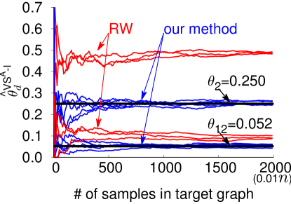
((a)) $\hat{\theta}^{VS\textsuperscript{A}\text{-I}}_{d}$

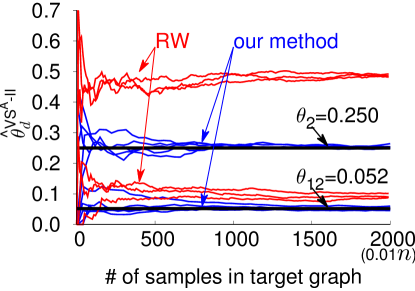
((b)) $\hat{\theta}^{VS\textsuperscript{A}\text{-II}}_{d}$

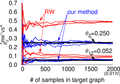
((c)) $\hat{\theta}^{RW\textsuperscript{T}VS\textsuperscript{A}}_{d}$ ($\alpha=10$)

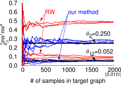
((d)) $\hat{\theta}^{RW\textsuperscript{T}RW\textsuperscript{A}}_{d}$ ($\alpha=\beta=10$)

Figure 9: Asymptotic unbiasedness of estimators.

Next, we study the estimation error of each estimator for estimating the PDF and CCDF of degree distribution. We choose the normalized rooted mean squared error (NRMSE) as a metric to evaluate the estimation error of an estimator, which is defined as follows

$$\text{NRMSE}(\hat{\theta})=\frac{\sqrt{\mathbb{E}[(\hat{\theta}-\theta)^{2}]}}{\theta}.$$

NRMSE measures the relative difference between an estimated value $\hat{\theta}$ and a real value $\theta$. The smaller the NRMSE, the more accurate the estimator $\hat{\theta}$ is. To compare the NRMSE of different estimators, we fix the sampling budget $B$ to be $1\%$ of the target graph size, and calculate the averaged empirical NRMSE over $1,000$ runs. The results are depicted in Figs. 10 and 11.

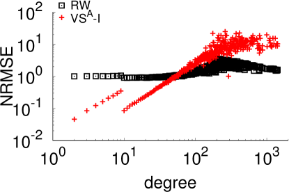
((a)) VS^A-I

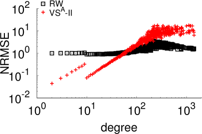
((b)) VS^A-II

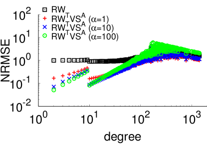
((c)) RW^TVS^A

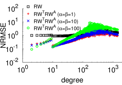
((d)) RW^TRW^A

Figure 10: PDF NRMSE of different estimators.

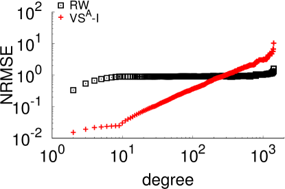
((a)) VS^A-I

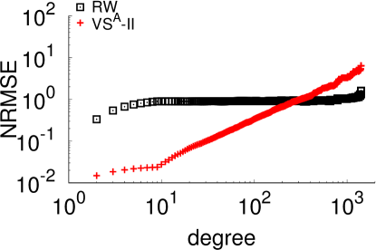
((b)) VS^A-II

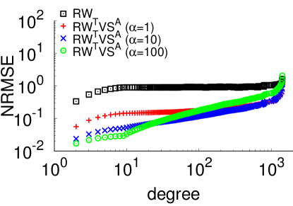
((c)) RW^TVS^A

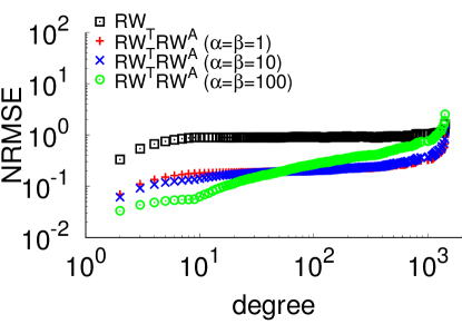
((d)) RW^TRW^A

Figure 11: CCDF NRMSE of different estimators.

To clearly see the performance difference, we also show the NRMSE of the random walk (RW) estimator as a baseline. Because a RW can hardly converge over a barbell graph within $B=0.01n$ steps, we observe that NRMSE of RW is almost the largest among all estimators for low degrees. Comparing VS^A-I and VS^A-II with RW, we find that the two VS^A estimators can provide smaller PDF/CCDF NRMSE for low degree nodes than RW. However, VS^A estimators produce larger NRMSE for high degree nodes than RW. Therefore, VS^A can better estimate low degree nodes than high degree nodes in a graph.

The weakness of VS^A can be overcome by RW^TVS^A and RW^TRW^A. From Fig. 11, it is clearer to see that when indirect jumps are incorporated into random walks in RW^TVS^A and RW^TRW^A, NRMSE for high degree nodes decreases, and NRMSE for low degree nodes remains smaller than RW. If we increase the probability of jumping at each step of random walk by increasing $\alpha$ and $\beta$, we observe that NRMSE for low degree nodes decreases, but NRMSE for high degree nodes increases. This behavior is similar to RWwJ [10, 13] and demonstrates that the indirect jumps in RW^TVS^A and RW^TRW^A indeed behave similarly as the direct jumps in RWwJs.

5.2 Experiments on LBSN Datasets

In the second experiment, we apply the VS^A-II method on two real-world LBSN datasets to solve the problem in Example 1, i.e., measure user characteristics in an area of interest on the map.

LBSN datasets. We obtain two public LBSN datasets from Brightkite and Gowalla [29]. Brightkite and Gowalla are once two popular LBSNs where users shared their locations by checking-in. Users in the two LBSNs are also connected by undirected friendship relations, which form two user social networks. The statistics of these two datasets are summarized in Table I.

TABLE I: Summary of two LBSN datasets.

[b] dataset Brightkite Gowalla $G$ network type undirected undirected users $58,228$ $196,591$ friendship edges $214,078$ $950,327$ users in LCC¹ $56,739$ $196,591$ edges in LCC $212,945$ $950,327$ $G^{\prime}$ and $G_{b}$ venues $772,966$ $1,280,969$ users having check-ins $51,406$ $107,092$ check-ins $4,491,143$ $6,442,890$ $G^{\prime}$ and $G_{b}$ for NYC venues in NYC² $23,484$ $26,448$ users checking in NYC $4,257$ $7,399$ check-ins in NYC $33,656$ $113,423$

• The largest connected component.

• The New York City (Fig. 12).

Because we are only interested in users that have check-ins, i.e., each node in the target graph connects to at least one node in the auxiliary graph, VS^A is applicable on these two datasets. Suppose that we want to measure characteristics of users located around New York City (NYC), which is specified by a rectangle region on a map: latitude range $40.4^{\circ}\sim 41.4^{\circ}$, longitude range $-74.3^{\circ}\sim-73.3^{\circ}$ (see Fig. 12). The goal is to estimate degree distribution of the users who checked in this region. As we explained in Introduction, directly sampling users is inefficient. Here, we apply the VS^A-II along with a venue sampling method — Random Region Zoom-In (RRZI) [25] to illustrate how to sample users in NYC more efficiently.

Figure 12: Venue distribution in New York City and illustration of accessible subregions used by RRZI. Each subregion contains less than $K$ venues.

Venue sampling. RRZI utilizes a venue query API provided by LBSNs to sample venues on a map. The API requires a user to specify a rectangle region by providing the south-west and north-east corners latitude-longitude coordinates, and then the API returns a set of venues in this region. Usually, the API can only return at most $K$ venues in a queried region. RRZI regularly zooms in the region until the subregion is fully accessible, i.e., the API returns less than $K$ venues in the subregion. The zooming-in process is equivalent to dividing the region into many non-overlapping accessible subregions, as illustrated in Fig. 12, and each subregion is associated with a fixed probability related to the zooming-in strategy. This feature enables RRZI to sample venues within an area of interest.

Results. Combining VS^A-II with RRZI, denoted by RRZI-VS^A, we conduct experiments on Brightkite and Gowalla to indirectly sample users in NYC. We totally sample $5\%$ of venues in NYC and calculate the degree distribution of users in NYC. The results are depicted in Fig. 13.

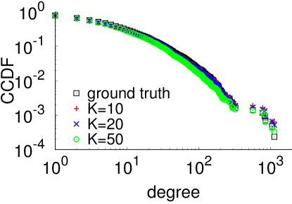
((a)) estimates (Brightkite)

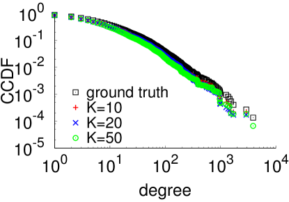
((b)) estimates (Gowalla)

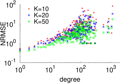
((c)) PDF NRMSE (Brightkite)

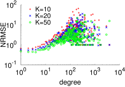
((d)) PDF NRMSE (Gowalla)

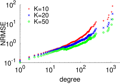
((e)) CCDF NRMSE (Brightkite)

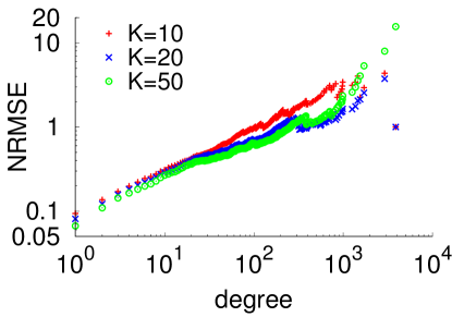
((f)) CCDF NRMSE (Gowalla)

Figure 13: Performance of RRZI-VS^A on Brightkite and Gowalla.

Figures 13(a) and 13(b) depict the estimates of CCDF with different query capacity $K$. We observe that our RRZI-VS^A method can provide good estimates of user characteristics in NYC on both datasets. Specifically, the estimates for low degree users are better than high degree users, and this is clear to see from the PDF/CCDF NRMSE plots. This feature coincides with our previous analysis using synthetic data. From the NRMSE plots, we can also find an approximate law that a larger query capacity $K$, i.e., the maximum number of venues the API can return, reduces the estimation error of RRZI-VS^A. However, it is not true for estimating high degree users on Gowalla in Fig. 13(f). In fact, a better way to reduce estimation error is to combine VS^A-II with other better venue sampling methods discussed in [23, 24, 25]. However, we have to omit this due to space limitation.

5.3 Experiments on Amazon Product Co-purchasing Network

In the third experiment, we compare the performance of VS^A-I and RW^TVS^A sampling methods on the Amazon product co-purchasing network.

Amazon product co-purchasing network. We build an Amazon product co-purchasing network from the Amazon dataset provided by [30]. The network is created based on “customers who bought this item also bought” feature of the Amazon website. That is, if a product $i$ is co-purchased with product $j$, the network contains an undirected edge between $i$ and $j$. In addition, each product belongs to at least one category on Amazon, and Amazon provides a complete category list on its homepage to facilitate customers to conveniently browse the products. Thus, we can leverage this category list to perform indirect sampling of the co-purchasing network. The detailed statistics of the Amazon dataset are provided in Table II.

TABLE II: Amazon product co-purchasing network statistics.

$G$	product co-purchasing network	undirected
	# of products	$4,015,942$
	# of co-purchases	$78,792,050$
$G^{\prime}$	# of categories	$10,164$
$G_{b}$	# of product-category associations	$15,829,046$
	avg. # of categories a product belongs to	$4$
	avg. # of products in a category	$1,557$

This dataset is suitable for us to study the performance of VS^A-I and RW^TVS^A, where the availability of the complete category list allows us to conduct uniform vertex sampling on the auxiliary graph. Here we sample $1\%$ of the nodes from target graph, and compare the accuracy of estimating PDF/CCDF degree distribution using different methods. The results are averaged over $1,000$ runs and are depicted in Fig. 14.

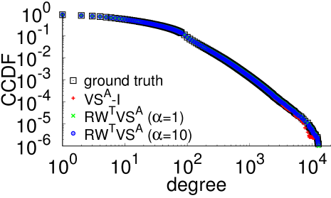
((a)) unbiasedness of CCDF estimates

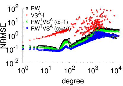
((b)) PDF NRMSE

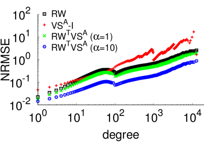
((c)) CCDF NRMSE

Figure 14: Amazon product co-purchasing network characterizing.

Results. From Fig. 14(a), we observe that the two methods can indeed provide unbiased estimates of the CCDF. From Figs. 14(b) and 14(c), we also observe that different methods have different estimation accuracy. In general, VS^A-I has relatively large estimation error, then comes the random walk estimator, and RW^TVS^A has the lowest estimation error among these three estimators. RW^TVS^A leverages the category list to perform indirect jumps on the target graph, and this approach can significantly improve the estimation accuracy. If we slightly increase $\alpha$ to increase the jumping probability, we observe that the estimation error further decreases.

5.4 Experiments on Mtime Dataset

In the fourth experiment, we apply RW^TVS^A and RW^TRW^A on Mtime to measure the Mtime user characteristics.

Mtime dataset. Mtime [31] is a popular online movie database in China, which comprises two types of accounts: Mtime users and movie actors. Mtime users can follow each other to form a social network, and movie actors can form connections with each other if they cooperated in the same movies. A Mtime user can follow movie actors if she is a fan of the actor. Suppose we want to measure Mtime user characteristics, then the relations between Mtime users and movie actors naturally form a two-layered network structure, where

• the target graph consists of Mtime users and their following relations;

• the auxiliary graph consists of movie actors and their cooperation relations;

• and the bipartite graph consists of Mtime users, movie actors and the fan relations between them.

To build a groundtruth dataset, we have collected the complete Mtime network by traversing Mtime user and movie actor ID spaces. For each Mtime user, we collect the set of users she follows and users who follow her. This builds up a directed follower network among Mtime users. Each Mtime user maintains a list including a subset of movie actors she is interested in. This information is used to build up the fan-relations between Mtime users and movie actors. For each movie actor, we collect the movies she participated in, and if two actors participated in a same movie, we connect them. This builds up a cooperative network among actors. The complete Mtime dataset is summarized in Table III.

TABLE III: Summary of the Mtime dataset

$G$	user follower network type	directed
	total users (isolated and non-isolated)	$1,878,127$
	non-isolated users in follower network	$1,035,164$
	following relations	$14,861,383$
	users in LCC	$987,055$
	following relations in LCC	$14,791,482$
$G^{\prime}$	actor cooperative network type	undirected
	total actors (isolated and non-isolated)	$1,123,340$
	non-isolated actors in cooperative network	$1,122,166$
	cooperative relations	$10,344,364$
	actors in LCC	$1,114,065$
	cooperative relations in LCC	$10,328,904$
$G_{b}$	fan relations	$225,558,343$
	users following actors	$1,419,339$
	isolated users following actors	$842,963$
	actors having fans	$441,413$
	isolated actors having fans	$1,174$
	isolated actors having only isolated fans	$225$
	isolated users following only isolated actors	$393$

Analysis of the dataset. First we provide some analysis about the Mtime dataset. In Table III, comparing the first block with second block, which are related to target graph $G$ and auxiliary graph $G^{\prime}$ respectively, we find that about $19\%$ of the user IDs and $93\%$ of the actor IDs are valid. This indicates that conducting UNI on the auxiliary graph is more efficient than conducting UNI on the target graph. Moreover, we find that more than $47\%$ of the Mtime users are not in LCC, but the number for actors is less than $0.1\%$. This indicates that the auxiliary graph is better connected than the target graph. Although a large fraction of users are isolated nodes in the target graph, from the last block, we find that almost all the isolated users are connected to non-isolated actors (except a few hundreds of them). So the majority of isolated users are indirectly connected to other users through actors. This is illustrated in Fig. 15. The advantage of introducing the two-layered network structure is now clear for Mtime dataset, i.e., we can study a larger user space than simply the LCC of target graph.

Figure 15: The Mtime network components. Dashed red lines denote fan relations between actors and users.

Results. Using the Mtime dataset as a testbed, we demonstrate that RW^TVS^A and RW^TRW^A methods can provide good estimates of user characteristics. Although the user follower network is directed, we can build an undirected version of the target graph on-the-fly while sampling because a user’s in-coming and out-going neighbors are known once the user is queried [11, 13]. Slightly different from previous experiments, here we will estimate both the in- and out-degree distributions.

Figure 16 depicts the results of RW^TVS^A. In Figs. 16(a) and 16(e), we show the in-degree and out-degree CCDF estimates. We can see that RW^TVS^A can provide unbiased estimates. From Figs. 16(b) and 16(f), we observe that when sampling budget increases, the NRMSE decreases for both in-degree and out-degree estimations. From Figs. 16(c) and 16(g) we observe that when more jumps are allowed by increasing $\alpha$ from $1$ to $100$, estimation accuracy also increases.

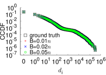
((a)) in-degree estimates ($\alpha=1$)

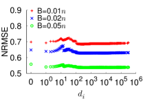
((b)) CCDF NRMSE ($\alpha=1$)

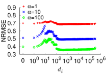
((c)) CCDF NRMSE ($B=0.01n$)

((d)) too frequent jumping ($B\!=\!0.01n$)

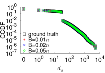
((e)) out-degree estimates ($\alpha=1$)

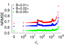
((f)) CCDF NRMSE ($\alpha=1$)

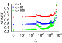
((g)) CCDF NRMSE ($B=0.01n$)

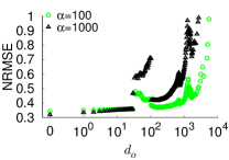
((h)) too frequent jumping ($B\!=\!0.01n$)

Figure 16: RW^TVS^A degree distribution estimation and NRMSE analysis.

Figure 17 depicts the results of RW^TRW^A, and they are similar to the results of RW^TVS^A. First, from Figs. 17(a) and 17(e), we observe that RW^TRW^A can also provide unbiased estimates of the in- and out-degree distributions. Second, from Figs. 17(b) and 17(f), we can find that as sampling budget increases, the estimation error decreases accordingly for both in- and out-degree estimations. Last, from Figs. 17(c) and 17(g), we find that when jumping probability increases (by increasing $\alpha$ and $\beta$), the NRMSE also decreases.

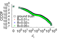
((a)) in-degree est. ($\alpha=\beta=0.1$)

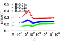
((b)) CCDF NRMSE ($\alpha=\beta=0.1$)

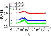
((c)) CCDF NRMSE ($B=0.01n$)

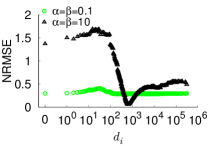
((d)) too frequent jumping ($B\!=\!0.01n$)

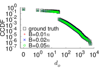
((e)) out-degree est. ($\alpha=\beta=0.1$)

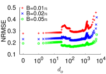
((f)) CCDF NRMSE ($\alpha=\beta=0.1$)

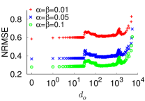
((g)) CCDF NRMSE ($B=0.01n$)

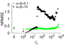
((h)) too frequent jumping ($B\!=\!0.01n$)

Figure 17: RW^TRW^A degree distribution estimation and NRMSE analysis.

However, it is worth noting that $\alpha$ and $\beta$ should not be too large for both RW^TVS^A and RW^TRW^A. Because we know that when $\alpha\rightarrow\infty$, RW^TVS^A becomes VS^A, which is biased on the Mtime dataset, and hence causes large NRMSE. Similar behavior happens to RW^TRW^A, too.

6 Related Work

We briefly review some related literature in this section.

Graph sampling methods, especially random walk based graph sampling methods, have been widely used to characterize large-scale complex networks. These applications include, but are not limited to, estimating peer statistics in peer-to-peer networks [32, 9], uniformly sampling users from OSNs [33, 12, 14, 15], characterizing structure properties of large-scale networks [34, 35, 36, 37], and measuring statistics of point-of-interests on maps [25]. The above literature is mostly concerned with sampling methods that seek to directly sample nodes (or samples) in target graphs (or some sample spaces). However, direct sampling is not always efficient as we argued in this work.

When the target graph (or sample space) can not be directly sampled or direct sampling is inefficient, several methods based on graph manipulation have been proposed to improve sampling efficiency. For example, Gjoka et al. [38] study an approach to improve sampling efficiency through building a multigraph using different kinds of relations (i.e., different types of edges) that exist on an OSN. A multigraph is better connected than any individual graph formed by only one kind of relations. Therefore, the random walk can converge fast on this multigraph. Zhou et al. [39] exploit several criteria to rewire the target graph on-the-fly to increase the graph conductance [16] and reduce mixing time of a random walk. Our method differs from theirs in that we do not manipulate target graphs. We study a new approach that utilizes a widely existed two-layered network structure to assist sampling on target graph indirectly.

Birnbaum and Sirken [40] designed a survey method for estimating the number of diagnosed cases of a rare disease in a population. Directly sampling patients of a rare disease from the huge human population is obviously inefficient, so they studied how to sample hospitals so as to sample patients indirectly. Their method motivates us to design the VS^A method. However, as we pointed out, VS^A method cannot sample nodes that are not connected to auxiliary graph, and we overcome this problem by designing RW^TVS^A and RW^TRW^A methods. Our work also complements existing sampling methods related to random walk with jumps [10, 13, 15] by removing the necessity of uniform node sampling on target graphs.

7 Conclusion

When graphs become large in scale, sampling methods become necessary tools in the study of characterizing their properties. Among these sampling methods, random walk-based crawling methods are effective and are gaining popularity. However, if the graph under study is not well connected, random walk-based graph sampling methods suffer from the slow mixing problem. In this work, we observe that a graph usually does not exist in isolation. In many applications, the target graph is accompanied with an auxiliary graph and a bipartite graph, and they together form a better connected two-layered network structure. This new viewpoint brings extra benefits to the graph sampling framework. We design three sampling methods to measure the target graph from this new viewpoint, and these methods are demonstrated to be effective on both synthetic and real datasets. Therefore, our method complements existing methods in the literature of graph sampling.

References

- [1] J. Leskovec, D. Huttenlocher, and J. Kleinberg, “Signed networks in social media,” in Proceedings of the SIGCHI Conference on Human Factors in Computing Systems, 2010.
- [2] B. Zhang, G. Kreitz, M. Isaksson, J. Ubillos, G. Urdaneta, J. A. Pouwelse, and D. Epema, “Understanding user behavior in spotify,” in Proceedings of the 32nd Annual IEEE International Conference on Computer Communications, 2013.
- [3] L. Backstrom and J. Kleinberg, “Romantic partnerships and the dispersion of social ties: A network analysis of relationship status on Facebook,” in Proceedings of the 17th ACM Conference on Computer Supported Cooperative Work and Social Computing, 2014.
- [4] H. Li, W. Ai, X. Liu, J. Tang, G. Huang, F. Feng, and Q. Mei, “Voting with their feet: Inferring user preferences from app management activities,” in Proceedings of the 25th International World Wide Web Conference, 2016.
- [5] J. Han, D. Choi, B.-G. Chun, T. T. Kwon, H. chul Kim, and Y. Choi, “Collecting, organizing, and sharing pins in Pinterest: Interest-driven or social-driven?” in Proceedings of the ACM Special Interest Group (SIG) for the computer systems performance evaluation community, 2014.
- [6] M. Mondal, B. Viswanath, P. Druschel, K. P. Gummadi, A. Clement, A. Mislove, and A. Post, “Defending against large-scale crawls in online social networks,” in Proceedings of the 8th International Conference on emerging Networking EXperiments and Technologies, 2012.
- [7] “Sina Weibo API rate limiting,” http://open.weibo.com/wiki/Rate-limiting, May 2017.
- [8] “Twitter API rate limiting,” https://dev.twitter.com/rest/public/rate-limiting, May 2017.
- [9] L. Massoulié, E. L. Merrer, A.-M. Kermarrec, and A. Ganesh, “Peer counting and sampling in overlay networks: Random walk methods,” in Proceedings of ACM Symposium on Principles of Distributed Computing, 2006.
- [10] K. Avrachenkov, B. Ribeiro, and D. Towsley, “Improving random walk estimation accuracy with uniform restarts,” in Proceedings of the 7th Workshop on Algorithms and Models for the Web Graph, 2010.
- [11] B. Ribeiro and D. Towsley, “Estimating and sampling graphs with multidimensional random walks,” in Proceedings of the 10th ACM SIGCOMM conference on Internet measurement conference, 2010.
- [12] M. Gjoka, M. Kurant, C. T. Butts, and A. Markopoulou, “Practical recommendations on crawling online social networks,” IEEE Journal on Selected Areas in Communications, vol. 29, no. 9, pp. 1872–1892, 2011.
- [13] B. Ribeiro, P. Wang, F. Murai, and D. Towsley, “Sampling directed graphs with random walks,” in Proceedings of the 31st Annual IEEE International Conference on Computer Communications, 2012.
- [14] C.-H. Lee, X. Xu, and D. Y. Eun, “Beyond random walk and Metropolis-Hastings samplers: Why you should not backtrack for unbiased graph sampling,” in Proceedings of the ACM Special Interest Group (SIG) for the computer systems performance evaluation community, 2012.
- [15] X. Xu, C.-H. Lee, and D. Y. Eun, “A general framework of hybrid graph sampling for complex network analysis,” in Proceedings of the 33rd Annual IEEE International Conference on Computer Communications, 2014.
- [16] A. Sinclair and M. Jerrum, “Approximate counting, uniform generation and rapidly mixing markov chains,” Information and Computation, vol. 82, no. 1, pp. 93–133, 1989.
- [17] A. Mohaisen, A. Yun, and Y. Kim, “Measuring the mixing time of social graphs,” in Proceedings of the 10th ACM SIGCOMM conference on Internet measurement conference, 2010.
- [18] “Pinterest,” http://www.pinterest.com, May 2017.
- [19] “Sina Weibo,” http://weibo.com, May 2017.
- [20] “Weibo place,” http://place.weibo.com, May 2017.
- [21] “Weibo search API,” http://open.weibo.com/wiki/2/location/pois/search/by_area, May 2017.
- [22] “Foursquare search API,” https://developer.foursquare.com/docs/venues/search, May 2017.
- [23] Y. Li, M. Steiner, L. Wang, Z.-L. Zhang, and J. Bao, “Dissecting Foursquare venue popularity via random region sampling,” in Proceedings of the 8th International Conference on emerging Networking EXperiments and Technologies, 2012.
- [24] Y. Li, L. Wang, M. Steiner, J. Bao, and T. Zhu, “Region sampling and estimation of geosocial data with dynamic range calibration,” in Proceedings of the 30th IEEE International Conference on Data Engineering, 2014.
- [25] P. Wang, W. He, and X. Liu, “An efficient sampling method for characterizing points of interests on maps,” in Proceedings of the 30th IEEE International Conference on Data Engineering, 2014.
- [26] S. Meyn and R. L. Tweedie, Markov Chains and Statistic Stability, 2nd ed. Cambridge University Press, 2009.
- [27] C. P. Robert and G. Casella, Monte Carlo Statistic Methods, 2nd ed. Springer, 2004.
- [28] A. L. Barabási and R. Albert, “Emergence of scaling in random networks,” Science, vol. 286, no. 5439, pp. 509–512, 1999.
- [29] E. Cho, S. A. Myers, and J. Leskovec, “Friendship and mobility: User movement in location-based social networks,” in Proceedings of the 17th ACM SIGKDD international conference on Knowledge discovery and data mining, 2011.
- [30] J. McAuley, R. Pandey, and J. Leskovec, “Inferring networks of substitutable and complementary products,” in Proceedings of the 21st ACM SIGKDD International Conference on Knowledge Discovery and Data Mining, 2015.
- [31] “Mtime,” http://www.mtime.com, May 2017.
- [32] C. Gkantsidis, M. Mihail, and A. Saberi, “Random walks in peer-to-peer networks: Algorithms and evaluation,” Performance Evaluation, vol. 63, no. 3, pp. 241–263, 2006.
- [33] M. Gjoka, M. Kurant, C. T. Butts, and A. Markopoulou, “Walking in Facebook: A case study of unbiased sampling of OSNs,” in Proceedings of the 29th Annual IEEE International Conference on Computer Communications, 2010.
- [34] L. Katzir, E. Liberty, and O. Somekh, “Estimating sizes of social networks via biased sampling,” in Proceedings of the 19th International World Wide Web Conference, 2011.
- [35] S. J. Hardiman and L. Katzir, “Estimating clustering coefficients and size of social networks via random walk,” in Proceeding of the 22nd International World Wide Web Conference, 2013.
- [36] C. Seshadhri, A. Pinar, and T. G. Kolda, “Triadic measures on graphs: The power of wedge sampling,” in Proceedings of the 13th SIAM International Conference on Data Mining, 2013.
- [37] P. Wang, J. C. Lui, B. Ribeiro, D. Towsley, J. Zhao, and X. Guan, “Efficiently estimating motif statistics of large networks,” ACM Transactions on Knowledge Discovery from Data, 2014.
- [38] M. Gjoka, C. T. Butts, M. Kurant, and A. Markopoulou, “Multigraph sampling of online social networks,” IEEE Journal on Selected Areas in Communications, vol. 29, no. 9, pp. 1893–1905, 2011.
- [39] Z. Zhou, N. Zhang, Z. Gong, and G. Das, “Faster random walks by rewiring online social networks on-the-fly,” in Proceedings of the 29th IEEE International Conference on Data Engineering, 2013.
- [40] Z. W. Birnbaum and M. G. Sirken, “Design of sample surveys to estimate the prevalence of rare diseases: Three unbiased estimates,” Vital and Health Statistics, vol. 2, no. 11, pp. 1–8, 1965.