Tensor network method for reversible classical computation

Abstract

We develop a tensor network technique that can solve universal reversible classical computational problems, formulated as vertex models on a square lattice [Nat. Commun. 8, 15303 (2017)]. By encoding the truth table of each vertex constraint in a tensor, the total number of solutions compatible with partial inputs/outputs at the boundary can be represented as the full contraction of a tensor network. We introduce an iterative compression-decimation (ICD) scheme that performs this contraction efficiently. The ICD algorithm first propagates local constraints to longer ranges via repeated contraction-decomposition sweeps over all lattice bonds, thus achieving compression on a given length scale. It then decimates the lattice via coarse-graining tensor contractions. Repeated iterations of these two steps gradually collapse the tensor network and ultimately yield the exact tensor trace for large systems, without the need for manual control of tensor dimensions. Our protocol allows us to obtain the exact number of solutions for computations where a naive enumeration would take astronomically long times.

I Introduction

Physics-inspired approaches have led to efficient algorithms for tackling typical instances of hard computational problems, shedding new light on our understanding of the complexity of such problems Mézard et al. (2002); Mezard and Montanari (2009). The conceptual framework of these approaches is based on the realization that the solutions of certain computational problems are encoded in ground states of appropriate statistical mechanics models. However, the existence of either a thermodynamic phase transition into a glassy phase or a first-order quantum phase transition represent obstructions to reaching the ground state, often even for easy problems Ricci-Tersenghi (2010); Jörg et al. (2010); Young et al. (2010); Hen and Young (2011); Farhi et al. (2012). Recently, Ref. Chamon et al. (2017) introduced a new class of problems by mapping a generic reversible classical computation onto a two-dimensional vertex model with appropriate boundary conditions. The statistical mechanics model resulting from this mapping displays no bulk thermodynamic phase transitions and the bulk thermodynamics is independent of the classical computation represented by the model. Taken together, these features remove an obvious obstacle to reaching the ground state of a large class of computational problems and imply that the time-to-solution and the complexity of the problem are determined by the dynamics of the relaxation of the corresponding system to its ground state. However, when thermal annealing is employed, the resulting dynamics is found to be extremely slow, and even easy computational problems cannot be efficiently solved. Since any classical computation implemented as a reversible circuit can be formulated in this fashion, finding an algorithm that can solve the resulting vertex models efficiently would have far-reaching repercussions.

In this paper, we introduce a tensor network approach that can treat vertex models encoding computational problems. Tensor networks are a powerful tool in the study of classical and quantum many-body systems in two and higher spatial dimensions, and are also used as compressed representations of large-scale structured data in “big-data” analytics Cichocki (2014a); Vervliet et al. (2014); Cichocki (2014b). Here we are interested in taking the trace of tensor networks Biamonte et al. (2013, 2015); Biamonte and Bergholm (2017), to count the number of solutions of a computational problem. As opposed to thermal annealing, which serially visits individual configurations, tensor network schemes sum over all configurations simultaneously. As a result, tensor-based approaches lead to a form of virtual parallelization Chamon and Mucciolo (2012), which, under certain circumstances, speeds up the computation of the trace. Most of the physics-driven applications have focused on tensor network renormalization group (TNRG) algorithms that coarse grain the network while optimally removing short-range entanglement Verstraete and Cirac (2004); Levin and Nave (2007); Gu et al. (2008); Jiang et al. (2008); Gu and Wen (2009); Evenbly and Vidal (2009); Xie et al. (2012); Evenbly and Vidal (2015); Zhao et al. (2016); Yang et al. (2017a); Bal et al. (2017); Liao et al. (2017); Evenbly (2017a); Goldsborough and Evenbly (2017). There are, however, two aspects of our physics-motivated work that are qualitatively different from that of TNRG approaches. First, vertex models of computational gates are intrinsically not translationally invariant. Second, the trace over the tensor network, which counts the number of solutions of the computational circuit (the analogue of the zero temperature partition function of statistical mechanics models) must be computed exactly, within machine precision. (Approximations of the tensors lead to approximate counting, which in certain problems is no easier than exact counting Feige et al. (1991).) Both features are naturally treated by the methods proposed in this paper.

In our tensor network approach, the truth table of each vertex constraint corresponding to a computational gate is encoded in a tensor, such that the local compatibility between neighboring bits (or spins) is automatically guaranteed upon contracting the shared bond between two tensors. Summing over all possible unfixed boundary vertex states and contracting the entire tensor network give the partition function, which counts the total number of solutions compatible with the boundary conditions, a problem belonging to the class #P. Finding a solution can then be accomplished by fixing one boundary vertex at a time, with the total number of trials linear in the number of input bits Chamon and Mucciolo (2012).

Our tensor network method, which we refer to as the iterative compression-decimation (ICD) algorithm, can be regarded as a set of local moves defining a novel dynamical path to the ground state of generalized vertex models on a square lattice. These moves can be shown to decrease or leave unchanged the bond dimensions of the tensors involved, thus achieving optimal compression (i.e., minimal bond dimension) of the tensor network on a lattice of fixed size. The algorithm’s first step is to propagate local vertex constraints across the system via repeated contraction-decomposition sweeps over all lattice bonds. These back and forth sweeps are the higher dimensional tensor-network analog of those employed in the one-dimensional finite-system density matrix renormalization group (DMRG) method Schollwöck (2005). For problems with non-trivial boundary conditions, such as those encountered in computation, these sweeps also propagate the boundary constraints into the bulk, thus progressively building the connection between opposite (i.e., input/output) boundaries. In the next step, the algorithm decreases the size of the lattice by coarse-graining the tensor network via suitable contractions. Repeated iterations of these two steps allow us to reach larger and larger system sizes while keeping the tensor dimensions under control, such that ultimately the full tensor trace can be taken.

The computational cost of ICD hinges upon the maximum bond dimension of the tensors during the coarse-graining procedure. We identify the hardness of a given counting problem by studying the scaling of the maximum bond dimension as a function of the system size, the concentration of nontrivial constraints imposed by TOFFOLI gates, and the ratio of unfixed boundary vertices. We further present both the average and typical maximum bond dimension distributions over random instances of computations. While we cannot distinguish between polynomial and exponential scaling for the hardest regime of high TOFFOLI concentration, there exist certain regimes of the problem where the bond dimension grows relatively slowly with system size. Therefore, within this regime, we are able to count the exact number of solutions within a large search space that is intractable via direct enumerations.

The rest of the paper is organized as follows. We first briefly introduce the tensor network representation of generic vertex models on a square lattice in Sec. II. Section III describes the ICD algorithm for coarse-graining and efficiently contracting the tensor network. In Section IV we apply the ICD method to reversible classical computational problems as encoded in the vertex model of computation introduced in Ref. Chamon et al. (2017), and discuss a relation between the number of solutions of the computational problem and the maximum bond dimension of the tensor network from an entanglement perspective. Section V presents the implementation of the ICD and the accompanying numerical scaling results for random computational networks defined by the concentration of Toffoli gates placed randomly at vertices of a tilted planar square lattice. Finally, we close with Sec. VI, where we outline future applications of our ICD algorithm to both computational and physics problems.

II Tensor network for vertex models

We start by introducing the tensor network representation for a generic vertex model. In our formulation, discrete degrees of freedom reside on the edges of a regular lattice and they are coupled locally to their neighboring degrees of freedom. Couplings between degrees of freedom are denoted by vertices. The couplings at each vertex $n=1,\ldots,N_{\mathrm{sites}}$, where $N_{\mathrm{sites}}$ denotes the total number of vertices, are encoded into a tensor $T[n]$ whose rank will depend on the connectivity of the lattice. Fixing the state at all edges incident to a vertex collapses the corresponding tensor to a scalar. For concreteness, let us consider the square lattice as an example, as shown in Fig. 1; generalizations to other types of lattices are straightforward. Each tensor $T[n]$ is therefore a rank-4 tensor $T[n]_{ijkl}$, where $i,j,k,l$ denote bond indices.

Figure 1: (Color online) Vertex model on a square lattice. A local tensor $T[n]_{ijkl}$ is defined on each lattice site.

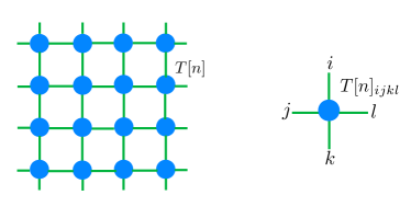
The tensor representation is quite general. If, for example, one associates a Boltzmann weight with each combination of bond index values, one can encode statistical mechanics problems into the tensor network Levin and Nave (2007); Gu et al. (2008); Xie et al. (2012); Evenbly and Vidal (2015); Zhao et al. (2016); Yang et al. (2017a). Alternatively, by assigning boolean 1s to “compatible” combinations of bond index values and boolean 0s to “incompatible” ones, such that the tensor represent a vertex constraint or a truth table, one can either study statistical mechanical vertex models at zero temperature, or implement computational circuits with the tensor network (Sec. IV). Finally, one could even embed the weights of a discretized path integral for a 1+1D quantum problem in a two-dimensional network. For finite systems with boundaries, the boundary tensors will have a different rank from the bulk tensors.

We define the tensor trace of the network as

$$Z={\rm tTr}\prod_{n}T[n]_{ijkl},$$ (1)

where $n$ runs over all lattice sites and tTr denotes full contractions of all bond indices. This trace may correspond to the partition function for the 2D classical system, or the number of possible solutions of a computation, or the imaginary-time path integral for a 1D quantum system, etc. In general, a brute-force evaluation of the full tensor trace multiplies the dimensions of the tensors, thereby requiring a number of operations exponential in system sizes. It is therefore expedient for any strategy of evaluating the trace to keep the dimensions of tensors under control at intermediate steps, so that the tensor trace can be ultimately taken. Ideally, one would like a protocol that uses all available information — such as boundary conditions, compatibility constraints, energy costs or Boltzmann weights, depending on the particular problem at hand — to compress the tensor network as much as possible, while maintaining all the essential information therein. In Sec. III, we propose an efficient iterative scheme that achieves this goal. In particular, as we detail in Sec. IV, our algorithm provides a simple way to deal with finite systems without translational invariance, and subject to various types of boundary conditions.

III compression-decimation algorithm

In this section, we describe the compression-decimation algorithm that facilitates the exact contraction of tensor networks. The algorithm consists of two steps. First, we perform sweeps on the lattice via a singular value decomposition (SVD) of pairs of tensors in order to eliminate short-range entanglement and propagate information from the boundary to the bulk, hence removing the redundancies in the bond dimensions. Due to its nature, we call this step compression. Next, we contract pairs of rows and columns of the lattice such that the system size is reduced. This step is referred to as decimation. The two steps are then repeated until the size and bond dimensions of the tensor network become small enough to allow an exact full contraction of the network.

Locally, the sweeps remove redundancies due to either short-range entanglement or incompatibility in the local tensors, and compress the information into tensors with smaller bond dimensions. Globally, the sweeps propagate information about the boundary conditions to the bulk, thus imposing global constraints on the local bulk tensors. Moreover, since the sweeping is performed back and forth across the entire lattice, it does not differentiate between whether or not translational invariance is present. Therefore, our scheme may be thought of as a higher dimensional analog of the finite-system DMRG algorithm that applies to generic vertex models on finite lattices.

III.1 Compression

In this step, we visit sequentially each bond in the lattice and contract the corresponding indices of the two tensors sharing this bond. We then perform an SVD on the contracted bond and truncate the singular value spectrum keeping only those greater than a certain threshold $\delta$. After that, the tensors are reconstructed with a smaller bond dimension. We define each forward plus backward traversal of all the bonds in the network as one sweep. The specific choice of the threshold $\delta$ depends on the desired precision, as well as the problem we are dealing with. For example, in formulating TNRG algorithms, $\delta$ can be chosen to be some small but finite number. On the other hand, for computational problems such as counting, $\delta$ is chosen to be zero within machine precision.

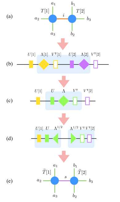
Let us take two tensors with the shared bond labeled by $i$, $T[1]_{a_{1}a_{2}a_{3}i}$ and $T[2]_{b_{1}ib_{2}b_{3}}$, as shown in Fig. 2a, where we denote the dimension of bond $i$ as $d_{i}$. We would like to reduce $d_{i}$ via a SVD. In principle, this can be achieved by directly contracting $T[1]$ and $T[2]$ along dimension $i$ into a matrix $M_{A,B}=T[1]_{A,i}T[2]_{i,B}$, where we have grouped the other three indices of each tensor into superindices $A\equiv(a_{1}a_{2}a_{3})$ and $B\equiv(b_{1}b_{2}b_{3})$, and then performing an SVD. However, to avoid decomposing the matrix $M_{A,B}$ with potentially large bond dimensions, we first do an SVD on each individual tensor (Fig. 2b):

$$T[1]_{A,i} = U[1]_{A,r}\,\Lambda[1]_{r}\,V[1]^{\intercal}_{r,i}\,,$$ (2a)

$$T[2]_{i,B} = U[2]_{i,r^{\prime}}\,\Lambda[2]_{r^{\prime}}\,V[2]^{\intercal}_{r^{\prime},B}.$$ (2b)

Notice that the contraction of $$T[1] T[2]$$ and can then be written as

$$T[1]T[2]=U[1]_{A,r}\bigg{[}\Lambda[1]_{r}V[1]^{\intercal}_{r,i}U[2]_{i,r^{\prime}}\Lambda[2]_{r^{\prime}}\bigg{]}V[2]^{\intercal}_{r^{\prime},B}.$$ (2c)

This implies that we can instead perform an SVD on the part shown within brackets in Eq. (2c): $$\widetilde{M}_{r,r^{\prime}}=\Lambda[1]_{r}V[1]^{\intercal}_{r,i}U[2]_{i,r^{\prime}}\Lambda[2]_{r^{\prime}} d_{r}\leq{\rm min}(d_{A},d_{i}),d_{r^{\prime}}\leq{\rm min}(d_{B},d_{i}) \widetilde{M}_{r,r^{\prime}}$$, which has much smaller dimensions since . Now we perform an SVD on the matrix to obtain (Fig. 2c)

$$\widetilde{M}_{r,r^{\prime}}=U_{r,s}\Lambda_{s}V^{\intercal}_{s,r^{\prime}}.$$ (2d)

(At each SVD step described above, we discard singular values that are smaller than $$\delta d_{s}\leq{\rm min}(d_{r},d_{r^{\prime}})\leq{\rm min}(d_{i},d_{A},d_{B})$$.) Therefore, after the above steps, the bond dimension . Finally, we construct new tensors as

$$\widetilde{T}[1]_{a_{1}a_{2}a_{3}s}\equiv {\ }\widetilde{U}_{(a_{1}a_{2}a_{3}),s}\,(\Lambda_{s})^{1/2}\,,$$ (2e)

$$\widetilde{T}[2]_{sb_{1}b_{2}b_{3}}\equiv {\ }(\Lambda_{s})^{1/2}\,\widetilde{V}^{\intercal}_{s,(b_{1}b_{2}b_{3})}\,,$$ (2f)

where the dimension of the shared bond is reduced (Fig. 2d,e). Starting from one boundary, we visit sequentially each bond $i\in 1,\ldots,N_{\mathrm{bonds}}$, where $N_{\mathrm{bonds}}$ is the total number of bonds in the lattice, and perform the steps outlined above, until we reach the opposite boundary. Then we repeat the procedure in the opposite direction, until we reach the original boundary. The sweeping can be repeated $N_{\mathrm{sweeps}}$ times, or until convergence of all bond dimensions.

Figure 2: (Color online) The contraction-decomposition step in the sweeping. (a) Two tensors $T[1]$ and $T[2]$ sharing a bond $i$. (b) Perform SVDs on individual tensors respectively. (c) Perform an SVD on the shaded part. (d) Split the resultant matrices into two pieces. (e) Construct new tensors $\widetilde{T}[1]$ and $\widetilde{T}[2]$.

III.2 Decimation

Figure 3: (Color online) (a) A column contraction involving pairs of tensors along the $x$ direction. (b) A row contraction involving pairs of tensors along the $y$ direction. The new tensors resulting from the contractions are denoted by pink dots, and the new bonds are denoted by orange lines.

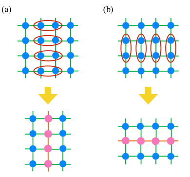
The second step of the algorithm is to contract pairs of rows and columns of the tensor network, so as to yield a lattice with a smaller number of sites Xie et al. (2012); Zhao et al. (2016). As we show in Fig. 3, this step consists of a column contraction (Fig. 3a), followed by a row contraction (Fig. 3b). In the column contraction, we contract pairs of tensors along the $x$ direction, and obtain a new tensor (see also Fig. 2a):

$$\mathcal{T}_{(a_{1}b_{1})a_{2}(a_{3}b_{2})b_{3}}=\sum_{i}T[1]_{a_{1}a_{2}a_{3}i}\,T[2]_{b_{1}ib_{2}b_{3}}.$$ (3)

We then perform a row contraction similarly, during which pairs of tensors are contracted along the $y$ direction.

During this step, the dimensions of the bonds perpendicular to the current direction of contractions are multiplied and hence will inevitably grow. Therefore, after all columns/rows are contracted, we sweep back and forth again to reduce the bond dimensions. A simplified version of the compression-decimation scheme is presented as pseudocode in Algorithm 1.

Algorithm 1 Iterative Compression-Decimation

Input: tensor network on a square lattice $\{T[n]\,|\,n\in 1,\dots,N_{\mathrm{sites}}\}$; $N_{\mathrm{sweeps}}\geq 1$; $\delta\geq 0$ (SVD truncation parameter).
Output: $Z$, as defined in Eq. (1)

1:repeat

2:     for $i=1,\ldots,N_{\mathrm{sweeps}}$ do (compression)

3:         for $b=1,\ldots,N_{\mathrm{bonds}}$ do (forward sweep)

4:              Contract, SVD, and update tensors as in Eq. 2

5:         end for

6:         for $b=N_{\mathrm{bonds}},\ldots,1$ do (backward sweep)

7:              Carry out backward sweep similarly

8:         end for

9:     end for

10:     Perform column contractions by Eq.(3) (decimation)

11:     Perform row contractions similarly (decimation)

12:until network is decimated to single site

13:Carry out tensor trace Eq. (1)

A few remarks are in order. First, the lattice structure lends us more flexibility with the coarse-graining step since one does not have to contract every pair of rows and columns. For example, in cases of systems without translational invariance, representing either disordered statistical mechanics models or models encoding computational circuits, the bond dimensions are in general not distributed uniformly across the entire lattice. One could then perform the contractions selectively on rows and columns containing mostly tensors with small bond dimensions while leaving the rest for the next coarse-graining step. In practice, one could set an appropriate threshold in the algorithm depending on the specific problems. Second, the procedure described here is closely related to the TNRG algorithms where the key is to optimally remove short-range entanglement at each RG step. For example, Ref. Yang et al. (2017a) proposes a loop optimization approach for TNRG. An important step in that method is to filter out short-range entanglement within a plaquette via a QR decomposition, which we believe should be equivalent to our SVD-based sweeping. Moreover, as shall be shown in Sec. V.3, the sweeps take into account the local environment around each tensor. The loop structure of short-range entanglement is eliminated (at least partially) when we visit each bond around the loop and sweep across the whole system. Whether or not more elaborate schemes Gu and Wen (2009); Evenbly and Vidal (2009); Xie et al. (2012); Evenbly and Vidal (2015); Zhao et al. (2016); Yang et al. (2017a); Bal et al. (2017); Liao et al. (2017); Evenbly (2017a); Goldsborough and Evenbly (2017); Evenbly (2017b) for taking into account the tensor environment can improve the performance of the sweeps in the ICD scheme will not concern us in this work: we will see that even the simple sweep protocol described above is sufficient for the solution of complex generic computational problems. Third, our procedure is more apt for systems without translational invariance, e.g., spin glasses. Finally, the computational cost scales as $O(\chi^{5})$ for the SVD steps, and $O(\chi^{7})$ for the tensor contraction steps, where $\chi$ is the maximum bond dimension of the tensors. Hence the computational cost of our compression-decimation algorithm scales as $O(\chi^{7})$.

IV The general TOFFOLI-based vertex model

In this section, we provide an example of a hard computational problem where our scheme can be applied to find solutions in cases that are otherwise intractable. The models we study here follow from the vertex model representation of reversible classical computations introduced in Ref. Chamon et al. (2017). We remark that this general vertex model can address generic satisfiability problems, a statement that follows from a series of results already documented in the literature:

1. The circuit satisfiability (CSAT) problem is NP-complete Cook (1971); Levin (1973);

2. The CSAT problem can be formulated in terms of reversible circuits Nielsen and Chuang (2004);

3. Any reversible circuit can be constructed using only TOFFOLI gates Nielsen and Chuang (2004);

4. Any reversible circuit constructed out of TOFFOLI gates can be mapped onto our vertex model representation, with the addition of an appropriate number of identity and swap gates Chamon et al. (2017).

Hence, our vertex model can encode other satisfiability problems such as 3-SAT, which can be mapped into CSAT. (Indeed, it is possible to program 3-SAT with $n$ variables and $m$ clauses into a vertex model using a lattice of size $n\times 2m$ pre .)

The vertex model is defined on a square lattice of finite size with periodic boundary conditions in the transverse direction, thus placing the model on a cylinder. Depending on the specific computation, different types of boundary conditions are imposed in the longitudinal direction. In addition, this model does not display translational invariance since different gates of the computational circuit are implemented by different vertices. This model can encode general computational problems, including any of the hard instances, and serves as an excellent candidate to benchmark the performance of our scheme.

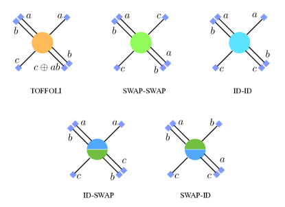
We start by giving a self-contained review of the general vertex model encoding reversible classical computations introduced in Ref. Chamon et al. (2017) and construct its tensor network representation. This is based on the fact that any Boolean function can be implemented using a reversible circuit constructed out of TOFFOLI gates, which are reversible three-bit logic gates taking the inputs $(a,b,c)$ to $(a,b,ab\oplus c)$. To facilitate the coupling of far-away bits while maintaining the locality of TOFFOLI gates, we use two-bit SWAP gates to swap neighboring bits, $(a,b)\rightarrow(b,a)$, until pairs of distant bits are adjacent to one another. Bits that do not need to be moved are simply copied forward using two-bit Identity (ID) gates. To obtain a plane-covering tiling and thus a square-lattice representation of the circuit, we combine the SWAP and ID gates into the three-bit gates: ID-ID, ID-SWAP, SWAP-ID, SWAP-SWAP, and represent each of them as well as the TOFFOLI gate as a vertex with three inputs and three outputs. The five types of vertices are shown in Fig. 4, with the input and output bits explicitly drawn on the links.

Figure 4: (Color online) Five types of vertices used for the vertex model representation of reversible classical computations. The input and output bits are denoted by blue squares on the links associated with a given vertex.

Alternatively, one can think of bits as spin 1/2 particles located on the bonds between vertices, whereas each vertex imposes local constraints between “input” and “output” spins, such that only $2^{3}=8$ out of the $2^{6}=64$ total configurations are allowed. For all five types of vertices, one can write local one- and two-spin interaction terms, such that the allowed configurations are given by the ground-state manifold of the Hamiltonian comprised of all these terms Chamon et al. (2017). The allowed configurations are then separated from the excited states by a gap set by the energy scale of the couplings. In the large-couplings limit, interactions can be equivalently thought of as constraints and one therefore needs only to consider the subspace where local vertex constraints are always satisfied.

Using the five types of vertices introduced above, one can map an arbitrary classical computational circuit onto a vertex model on a tilted square lattice, as shown in Fig. 5.

Figure 5: (Color online) Vertex model on a tilted square lattice encoding a generic classical computation. The left and right boundaries stores the input and output states, and periodic boundary condition is taken along the transverse direction.

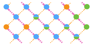
Bits at the left and right boundaries store the input and output respectively, and the horizontal direction corresponds to the computational “time” direction. The boundary condition along the transverse direction is chosen to be periodic. Spin degrees of freedom representing input and output bits associated with each vertex are placed on the links. This model can be shown to display no thermodynamic phase transition irrespective of the circuit realizations via a straightforward transfer matrix calculation Chamon et al. (2017).

When either only the input or only the output boundary bits are fully determined a priori, the physical system functions as a regular circuit: the solution can be obtained by passing the boundary state through the next column of gates, obtaining the output, then passing this output on to the next column of gates, repeating the procedure until the other boundary is reached. This mode of solution, which we shall call direct computation, is trivial and its computational cost scales linearly with the area of the system.

On the other hand, by fixing only a subset of the left and right boundaries, a class of nontrivial problems can be encoded in the vertex model. For example, one can cast the integer factorization problem on a reversible multiplication circuit precisely in this way Chamon et al. (2017); Vedral et al. (1996). In these cases, the boundary state cannot be straightforwardly propagated from the boundaries throughout the entire bulk, as the input or output of one or more gates is at most only partly fixed, and therefore direct computation unavoidably halts. Without any protocol of communication between the two partially fixed boundaries, one is left with trial-and-error enumeration of all boundary configurations, whose number grows exponentially with the number of unfixed bits at the boundaries. Even though it is sometimes possible to exploit special (nonuniversal) features of specific subsets of problems in order to devise efficient strategies of solution (e.g., factorization with sieve algorithms), general schemes that perform favorably in solving the typical instances in the encompassing class are important, both for highlighting the underlying universal patterns and as launchpads towards customized solvers for particular subsets of problems. The algorithm introduced in this work is of the latter general kind.

IV.1 Tensor network representation

We shall now construct a tensor network representation of the vertex model, such that the full contraction of the tensors yields the total number of solutions satisfying the boundary conditions. In the statistical mechanics language, this is the partition function of the vertex model at zero temperature, which essentially counts the ground state degeneracy.

Bulk tensors. We define a rank-4 tensor associated with each vertex in the bulk, $T_{ijkl}$, as shown in Fig. 6a. The tensor components are initialized to satisfy the truth table of the vertex constraint, meaning that $T_{ijkl}=1$ if $(ij)\rightarrow(kl)$ satisfies the vertex constraint, and $T_{ijkl}=0$ otherwise. Here the indices should be understood as integers labeling the spin (bit) states on each bond. Notice that the indices $i,l$ correspond to double bonds on the lattice while $j,k$ correspond to single bonds. Therefore, the original bond dimensions of the indices $(i,j,k,l)$ are $(4,2,2,4)$.

For concreteness, let us give an example of encoding the truth table of the TOFFOLI gate into the tensor $T_{ijkl}$. First, recall that the gate function of TOFFOLI is $(a,b,c)\rightarrow(a,b,d=c\oplus ab)$. Comparing Fig. 6a with Fig. 4, we identify on the input side, $i\equiv(ab)=2^{1}b+2^{0}a,j=c$; on the output side, $k=a,l\equiv(bd)=2^{1}d+2^{0}b$. In Table 1, we explicitly list the truth table of the TOFFOLI gate and its corresponding non-zero tensor components. All unspecified tensor components are set to zero. Tensors encoding the other four types of vertex constraints can be obtained in a similar fashion.

input			output			tensor component
$a$	$b$	$c$	$a$	$b$	$d$	$T_{ijkl}\equiv T_{(ab)ca(bd)}$
0	0	0	0	0	0	$T_{0000}=1$
0	0	1	0	0	1	$T_{0102}=1$
0	1	0	0	1	0	$T_{2001}=1$
0	1	1	0	1	1	$T_{2103}=1$
1	0	0	1	0	0	$T_{1010}=1$
1	0	1	1	0	1	$T_{1112}=1$
1	1	0	1	1	1	$T_{3013}=1$
1	1	1	1	1	0	$T_{3111}=1$

Table 1: Truth table and the corresponding tensor components for the TOFFOLI gate. On the input side, $i\equiv(ab)=2^{1}b+2^{0}a,j=c$; on the output side, $k=a,l\equiv(bd)=2^{1}d+2^{0}b$. All unspecified components are zero.

Boundary tensors. The vertices at the boundary have only two bonds. Hence we define a rank-2 tensor $T_{ij}$ at the boundary, where the indices $i,j$ have the same meaning as the bulk tensors (Fig. 6b). Here we draw a distinction between boundary tensors whose vertex states are fixed and those that are not. For fixed boundary vertices, $T_{ij}=1$ only for one component corresponding to the fixed state, whereas for unfixed ones, $T_{ij}=1\,\forall\,i,j$.

Figure 6: (Color online) Definition of (a) bulk and (b) boundary tensors.

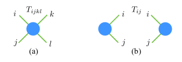
Under the above definitions of local tensors, local compatibility between spins shared by two vertices is automatically guaranteed when contracting the corresponding two tensors. Moreover, the unfixed boundary tensors already encode the information of all possible vertex states in a compact way, fulfilling a form of classical virtual parallelization Chamon and Mucciolo (2012). Therefore, the full contraction of the tensor network — if it can be performed — will give the total number of solutions subject to a certain boundary condition.

IV.2 Entanglement and number of solutions

Before moving on to the concrete application of the algorithm, let us try to gain some insights into the bond dimensions of local tensors needed to encode the information of the total number of solutions from an entanglement point of view Chamon and Mucciolo (2013). Let us denote the collection of free vertex states at the input and output boundaries by $\{q_{{\rm in}}\}$ and $\{q_{{\rm out}}\}$. We construct a weight $W(\{q_{{\rm in}},q_{{\rm out}}\})$ which equals 1 if the state $\{q_{\rm in},q_{\rm out}\}$ is a solution, and 0 otherwise. The partition function is then given by

$$Z=\sum_{\{q_{\rm in},q_{\rm out}\}}W(\{q_{{\rm in}},q_{{\rm out}}\}),$$ (4)

which equals the total number of solutions. Now we construct a quantum state as follows:

$$|\psi\rangle = \sum_{\{q_{{\rm in}},q_{{\rm out}}\}}W(\{q_{{\rm in}},q_{{\rm out}}\})\ |\{q_{{\rm in}},q_{{\rm out}}\}\rangle$$ (5)

$$= \sum_{\{q_{{\rm in}},q_{{\rm out}}\}}{\rm tTr}\left(T[1]^{q_{\rm in1}}T[2]^{q_{\rm in2}}\dotsb T[i]T[i+1]\dotsb T[N]^{q_{{\rm out}L_{\partial}}}\right)\ |\{q_{{\rm in}}\},\{q_{{\rm out}}\}\rangle,$$

where $N$ is the total number of vertices, $L_{\partial}$ is the number of unfixed vertices on each boundary, and tTr denotes tracing over all internal indices of the tensors. Let us imagine taking a cut perpendicular to the periodic direction and divide the system into two subsystems. The entanglement between subsystem left and right is determined by the singular value spectrum of the matrix $\mathcal{W}(\{q_{{\rm in}}\},\{q_{{\rm out}}\})$ reshaped from the weight $W(\{q_{{\rm in}},q_{{\rm out}}\})$. $\mathcal{W}$ is a matrix whose entries are either 1 or 0, and there can be at most one entry in each row and column that equals 1 due to the reversible nature of the circuit. Thus the rank of the matrix $\mathcal{W}$ is $Z$, and the zeroth-order Rényi entropy $S^{(0)}={\rm ln}Z$. The entanglement entropy of the quantum state (5) is hence upper bounded by $S^{(1)}\leq S^{(0)}={\rm ln}Z$. Therefore, at least when there is only a small (nonextensive) number of solutions, the amount of entanglement is low and the information can be encoded in tensors with small bond dimensions.

It may seem from the above argument that in the opposite limit of a large (extensive) number of solutions, the bond dimensions would necessarily be large. However, this is not true in general. Consider the open boundary condition under which every locally compatible configuration is a solution. In this extreme limit, the quantum state (5) is an equal amplitude superposition of all configurations, i.e., a product state. Such a state can be represented with tensors of bond dimension one in the ‘$x$-basis’. One thus expects that in cases of many solutions, the state should also be close to a product state with low entanglement, and hence can be represented with tensors of small bond dimensions. The above arguments indicate that, if there is a highly entangled regime where the bond dimensions required to represent the solution are large, then it must necessarily be for systems with an intermediate number of solutions. In Sec. V.3, we show numerically that, even in the intermediate regime where the solutions of an arbitrary vertex model are more than just a few, it is possible to obtain an efficient and compressed tensor network representation of the allowed-configuration manifold.

Having argued that, for the case of problems with a small number of solutions, solutions of vertex models with partially fixed boundaries can be encoded into tensor networks with small bond dimensions, we set out to find this tensor-network representation. The pertinent motivating question is: given that there is a representation that can compress the full information of all solutions with relatively small bond dimensions, how can we find it efficiently?

V Application of the ICD to the Random Vertex Model

In this section we apply ICD to $N$ random instances of vertex lattices of fixed concentration of TOFFOLI gates, and fixed and equal concentrations of all four other types of gates shown in Fig. 4, with random input states for each instance. By evaluating the full tensor trace for each of these $N$ instances and for various lattice sizes, we obtain information about the average scaling of performing the underlying classical computations by means of the ICD method. Moreover, we study the full distribution of the maximum bond dimension $\chi$ over random realizations and find that the typical behavior is generally different than the average, due to the presence of heavy tails in the bond-dimension distribution. Finally, we establish numerically that the scaling of the actual running time $\tau$ with the maximum bond dimension is always better than the worst-case estimate $\tau\sim\mathcal{O}(\chi^{7})$.

V.1 Local moves

Since the vertex model is defined on a tilted square lattice, we first need to turn it into a lattice as shown in Fig. 1 in order to apply our algorithm in Sec. III. This can be done by performing local moves on the tilted lattice, which we explain below.

Figure 7: (Color online) Illustration of the local moves which turn the original lattice into a square lattice rotated by $45^{\circ}$. In (a), sites belonging to sublattice $A$ and $B$ are shown in blue and green dots, respectively. From (b) to (c), four sites belonging to a diamond are contracted into one.

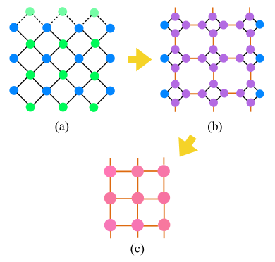
The tilted square lattice Fig. 7a is bipartite, with two sublattices A and B. Local tensor decompositions and contractions for tensors on each sublattice can rearrange the lattice into an “untilted” one, rotated by $45^{\circ}$ with respect to the original lattice. We start by splitting each tensor on the original vertex lattice into two along either horizontal or vertical direction, depending on which sublattice the corresponding site belongs to. Let us take a bulk tensor $T_{ijkl}$ on the original lattice. If the site belongs to sublattice $A$, we decompose the tensor horizontally into two rank-3 tensors, $T_{ijkl}=\sum_{q}A_{ijq}\,B_{klq}$; if the site belongs to sublattice $B$, we instead decompose the tensor vertically, $T_{ijkl}=\sum_{q}\widetilde{A}_{ikq}\,\widetilde{B}_{jlq}$, as shown in Fig. 8. Such a decomposition can be achieved via an SVD on the original tensors, $T_{(ij),(kl)}=U_{(ij),q}\,\Lambda_{q}\,V^{\intercal}_{q,(kl)}$ to yield $A_{ijq}=U_{(ij),q}\,(\Lambda_{q})^{1/2}$ and $B_{klq}=(\Lambda_{q})^{1/2}\,V^{\intercal}_{q,(kl)}$. We visit each site and split the tensors in this way. This turns the tensor network into the structure shown in Fig. 7b. We then further contract four tensors in a diamond into one and finally arrive at a new square lattice rotated by $45^{\circ}$ with respect to the original one (Fig. 7c). With these local moves, which have to be carried out only once, we cast the problem into the form discussed in Sec. II.

Figure 8: (Color online) Local moves that decompose each tensor on the original lattice into two along either horizontal or vertical direction, depending on whether the site belongs to sublattice A (a) or B (b).

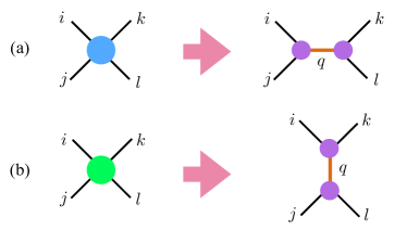
However, instead of doing an SVD on the original tensor, here we can use the fact that the tensors encode the truth tables of reversible gates and use an alternative method. Define a new set of tensors with an auxiliary index $q=0,1,\dotso,7$ labeling the vertex state, $\widetilde{T}^{q}_{ijkl}$. Now the component of this rank-(4,1) tensor is one if and only if $q$ is the same as the input state labeled by $(i,j)$. Then, the desired decomposition can be achieved as follows:

$$A_{ijq}=\sum_{kl}\widetilde{T}^{q}_{ijkl},\ \ \ B_{klq}=\sum_{ij}\widetilde{T}^{q}_{ijkl},$$

$$\widetilde{A}_{ikq}=\sum_{jl}\widetilde{T}^{q}_{ijkl},\ \ \ \widetilde{B}_{jlq}=\sum_{ik}\widetilde{T}^{q}_{ijkl}.$$ (6)

One can easily check that the contraction of the $A$ and $B$ tensors gives back the original tensor $T$, and hence this achieves the splitting shown in Fig. 8. The remaining steps of the algorithm are carried out exactly in the same way as before. By construction, the bonds between the resulting bulk tensors all have dimension 8.

V.2 Control of bond dimensions

We can now apply the compression-decimation algorithm to count the number of solutions for a given boundary condition. As we discuss in Sec. III.1, a truncation threshold $\delta$ needs to be specified in the sweeping step of the algorithm. Since we are performing an exact counting, no approximation in the truncation of the bond dimensions is made during the coarse-graining procedure, i.e., we choose $\delta=0$ within machine precision. This is a key methodological difference of the ICD to TNRG methods, which approximate physical observables to within a certain accuracy by enforcing a finite $\delta$.

As mentioned above, from a statistical mechanics point-of-view, what we are computing is the zero-temperature partition function of the vertex model, which yields the ground state degeneracy. In the bulk, all locally compatible configurations are equally possible until they receive information from the boundary conditions. Therefore, the coarse-graining step effectively brings the boundaries close to one another, and the sweeping step propagates information from the boundary to the bulk and knocks out states encoded in local tensors that are incompatible with the global boundary conditions.

The reason why the growth of bond dimensions remains controlled is that longer-range compatibility constraints over increasingly larger areas are enforced upon the coarse-grained tensors. These constraints are propagated to neighboring coarse-grained tensors upon sweeping, thus further reducing bond dimensions and compressing the tensor-network representation. For the trivial cases of either fixing all gates on one boundary or leaving them all free (open boundary condition), we have checked that the tensors converge to bond dimension one (scalars) after one sweep, without the need of coarse-graining. The tensor contraction is then simply reduced to multiplications of scalars, which can be trivially computed and indeed gives the correct counting. This demonstrates that the sweeping is responsible for propagating information from the boundary, and that the case of fully fixing one boundary is thus equivalent to direct computation, as described in Sec. IV.

In cases of mixed boundary conditions, the sweeping on the original lattice scale will generally not be sufficient to propagate information across the whole system or establish full communications between the two boundaries. Thus one would expect that while the bond dimensions close to the boundary may be small, those deep in the bulk may be large. We therefore perform the contractions selectively on rows and columns containing mostly tensors with small bond dimensions while leaving the rest for the next coarse-graining step, as described in Sec. III.

V.3 Numerical results

The computational cost of the ICD algorithm is determined by the maximum bond dimension encountered during the coarse-graining and sweeping procedures. In this section, we study the scaling of the maximum bond dimension as function of the set of parameters defining an instance of the problem: the number of vertices in each column $L$, the total number of columns (circuit depth) $W$, the concentration of TOFFOLI gates $c$, and the number of unfixed boundary vertices $L_{\partial}$. For a given set of parameters, we consider random tensor networks corresponding to typical instances of computational problems. By looking at the scaling of the bond dimensions, we gain some understanding of how the hardness of the problems depends on various parameters, which may serve as a guidance for designing and analyzing computational circuits for practical problems.

Figure 9: (Color online) The average bond dimension of the entire lattice as a function of the number of sweeps in the compression-decimation steps. The bumps where the average bond dimension increases slightly correspond to the points where we coarse-grain the lattice via column and row contractions. Inset: zoom-in plot from the 20th sweeping step.

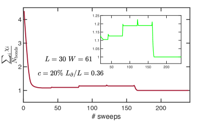
Before looking into the scaling of the maximum bond dimensions, we first show the average bond dimension for the entire lattice as a function of the number of sweeps in the compression-decimation steps. As seen from Fig. 9, the average bond dimension indeed decreases as the sweeping is performed. The bumps in the plot correspond to the points where we coarse-grain the lattice via column and row contractions. At a given length scale, the average bond dimension converges after a few sweeps. As we increase the length scales, the average bond dimension may first increase, but will eventually drop again as we perform sweeps at the new length scale. This demonstrates that the sweeping is able to impose global constraints at the boundary into the bulk, hence keeping the bond dimensions of bulk tensors under control.

We expect the maximum bond dimension to follow the scaling function $\chi=\mathcal{G}(L_{\partial}/L,c,L,W/L)$. Below we study the growth of maximum bond dimensions as a function of each system parameter numerically. First, we consider the scaling of $\chi$ as the ratio of unfixed boundary vertices $L_{\partial}/L$ is varied, with the other parameters fixed. As shown in Fig. 10a, the bond dimensions are small for both small and large $L_{\partial}/L$. This is in agreement with our discussions in Sec. IV.2, where we argued that in both regimes the states are close to product states and there should exist a representation in which the bond dimensions are small (the ‘$z$-basis’ and ‘$x$-basis’). For intermediate values of $L_{\partial}/L$, the bond dimensions grow, indicating the existence of a hard regime where either there is no such a representation of small bond dimensions to fully encode the solutions, or it is very hard to find such a representation via tensor optimization algorithms.

Figure 10: (Color online) Scaling of the average maximum bond dimension $\chi$ with (a) the ratio of unfixed boundary vertices $L_{\partial}/L$, and (b) TOFFOLI concentration $c$, versus the scaling of the typical maximum bond dimension $e^{\langle{\rm ln}\chi\rangle}$. The remaining parameters are fixed in each plot. The data are obtained by averaging over 2000 realizations of random tensor networks.

Figure 11: (Color online) Scaling of the average maximum bond dimension $\langle\chi\rangle$ with $L$ (a,b) and $W/L$ (c,d), versus the scaling of the typical maximum bond dimension $e^{\langle{\rm ln}\chi\rangle}$. The data are obtained by averaging over 500 to 2000 realizations of random tensor networks. In (a), the last point is averaged over 7 realizations and the error bar is not shown. The blue dotted line is a guide to the eye, and corresponds to a quadratic fitting. In all cases, the typical values stay below the average values, due to the presence of heavy tails in the distribution of $\chi$.

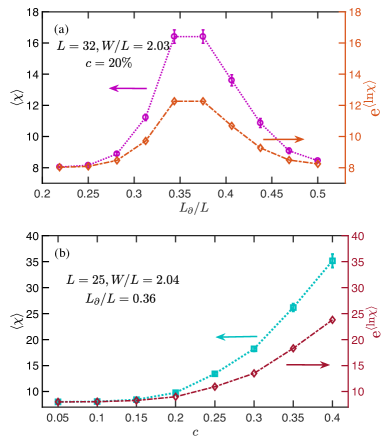
Fixing $L_{\partial}/L=0.36$, which corresponds to the hard regime in Fig. 10a, we plot the scaling of $\chi$ as a function of the TOFFOLI concentration $c$. The TOFFOLI gates impose nontrivial vertex constraints, which involve a nonlinear relationship between the input and output bits. In fact, in the absence of TOFFOLI gates, the vertex model can be expressed as $3L$ decoupled Ising chains whose dynamics are simple Chamon et al. (2017). In the ICD algorithm, the maximum bond dimension indeed grows with increasing TOFFOLI concentrations, as depicted in Fig. 10b.

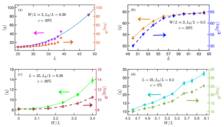
Now let us look at the scaling of $\chi$ as a function of the input size $L$. Again, we fix $L_{\partial}/L=0.36$ to stay in the hard regime. Figure 11a shows that the maximum bond dimension increases with increasing input size, even when the aspect ratio $W/L$ of the circuit is fixed. Because of the limited range of $L$ we were able to analyze, we cannot draw any conclusion regarding the functional form of this scaling, which would determine the complexity of our algorithm. However, we can demonstrate that our algorithm is able to solve the problem in regimes that are still intractable using a naive enumeration of solutions. For this purpose, we move away from the hardest regime and choose $L_{\partial}/L=0.5$. As can be seen in Fig. 11b, we are able to reach much larger values of $L$ in this regime, and the bond dimensions, although still growing, increase at a much slower pace. In fact, we were able to reach $L=96$ with an average maximum bond dimension $\langle\chi\rangle=78.25$ (data not shown). Since half of the input vertices are unknown, a direct trial-and-error enumeration would take $8^{48}\approx 10^{43}$ iterations to perform an exact counting, which is prohibitive even with parallelization. We have thus shown that there is a subset of nontrivial problems that can easily be solved by the ICD method, for which (a) direct enumeration is impossible to scale up and (b) efficient custom algorithms are not known.

Finally, we show the scaling with the aspect ratio $W/L$. As we previously discussed, the key to the reduction of the bond dimensions of bulk tensors is the global constraint imposed at the boundary. The coarse-graining step brings the boundaries close together while the sweeping step helps propagate information. Therefore, one should expect the problem to become harder as the circuit depth $W$ increases for a fixed $L$, since it takes more iterations of coarse-graining for the connection between the boundaries to be built, all the while the bond dimensions of the bulk tensors barely decrease. In Fig. 11c we show the scaling of $\chi$ as a function of $W/L$ in the hard regime; $\chi$ indeed grows upon increasing $W/L$, as expected. For computational problems of practical interests, the vertex model representation often has the feature of low TOFFOLI concentration but large aspect ratio, e.g., the multiplication circuit Chamon et al. (2017); Vedral et al. (1996). In Fig. 11d we show data for cases with this feature by lowering the TOFFOLI concentration to $c=5\%$ and keeping $L_{\partial}/L=0.5$. We find that the bond dimensions grow in a similar fashion as in Fig. 11c, although a larger range of values of $W/L$ now becomes amenable.

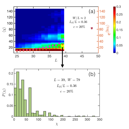
The above results demonstrate the average scaling behavior of the ICD algorithm over random instances of computations. It is informative to compare this to the typical behavior, revealed by analyzing the full distribution of the maximum bond dimensions; see, e.g., Fig. 11(a). In Fig. 12, we present the probability distribution of the maximum bond dimension. A vertical cut at each $L$ corresponds to the probability distribution over all instances for that $L$. For larger $L$ we observe secondary peaks at larger $\chi$, which gradually take up more weight, thus shifting both average and typical maximum bond dimension to higher values. Moreover, despite the fact that the highest weight is always encountered at small bond dimensions, a finite subset of hard instances generate much larger bond dimensions, leading to heavy tails in the distributions. Average values are sensitive to such tails, and hence do not faithfully represent the typical instances. In Fig. 10 and 11, we also plot the values of $e^{\langle{\rm ln}\chi\rangle}$ as an estimate of the typical behavior, in contrast to $\langle\chi\rangle$. Indeed, the typical values stay below the average values in all cases studied. We point out that the presence of heavy tails in the distribution is ubiquitous in random satisfiability problems, and such instances could in principle be tackled with different strategies Crosson et al. (2014); Steiger et al. (2015); Wecker et al. (2016); Yang et al. (2017b).

Figure 12: (Color online) The full distribution of the maximum bond dimension over random instances. In (a), the color plot along the vertical direction shows the probability distribution at each $L$. The orange (diamond) points show the values of $e^{\langle{\rm ln}\chi\rangle}$, giving an estimate of the typical instances in contrast to the average instances depicted in purple (triangle) points. In (b), we take the slice of $L=39$ in (a) and plot the histogram of the distribution.

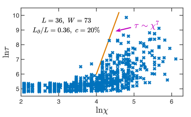
The efficiency of the ICD algorithm is controlled by the maximum bond dimension encountered in each instance, and in particular, the complexity of the algorithm is upper bounded by $\mathcal{O}(\chi^{7})$ as discussed in Sec. III. Nevertheless, it is still useful to see whether the actual running time saturates this bound. In Fig. 13 we show the scatter plot for the actual running time $\tau$ versus $\chi$ for 4600 random instances. We see a clear clustering of the data points and a positive correlation between these two quantities. The fact that there is a spreading of $\tau$ for each $\chi$ can be understood by taking into account the nonuniform spatial distributions of the bond dimensions across the system. Unlike the TNRG algorithms, where the bond dimensions of all tensors and all tensor legs are frequently chosen to be uniform, bond dimensions of different tensors and of different legs of the same tensor are typically highly nonuniform in the ICD method. Therefore, running times for instances with the same maximum $\chi$ also depend on the number of bonds with dimension $\chi$. The distribution of $\chi$ throughout the system is thus an important factor. Moreover, we find that the scaling of the running time with the maximum bond dimension $\tau\sim\chi^{\alpha}$ has a power $\alpha<7$, which shows that the actual performance of the algorithm is generally better than the worst-case scenario estimate.

Figure 13: (Color online) Scatter plot of the (logarithm of) actual running time $\tau$ in units of seconds versus the (logarithm of) maximum bond dimension $\chi$ for 4600 instances. The calculations were performed using a Python implementation of the ICD algorithm, using NumPy / LAPACK for all linear algebra operations, on 2.0 GHz Intel Xeon Processors E7-4809 v3.

VI Summary and outlook

We presented a method for contracting tensor networks that is well suited for the solution of statistical physics vertex models of universal classical computation. In these models, the tensor trace represents the number of solutions. Individual solutions can be efficiently extracted from the tensor network when the number of solutions is small. More generally, the method applies to any system, classical or quantum, whose quantity of interest is a tensor trace in an arbitrary lattice.

Our scheme consists of iteratively compressing tensors through a contraction-decomposition operation that reduces their bond dimensions, followed by decimation, which increases bond dimensions but reduces the network size. By repeated applications of this two step process – compression followed decimation – one can gradually collapse rather large tensor networks.

In the context of computation, the method allowed us to study relatively large classical reversible circuits represented by two dimensional vertex models. By contrast with thermal annealing, direct computation from a fully specified input boundary through the use of tensor networks occurs in a time linear in the depth of the circuit. For complex problems with partially fixed input/output boundaries tensor networks enable us to count solutions in problems where enumeration would otherwise take of order $8^{50}$ operations.

We close with an outlook of future directions motivated by this work.

First, focusing on the method per se, the performance of our ICD algorithm could still be further improved. There are enhancements that are simply operational in nature, such as parallelization of the sweeping step of the algorithm, which can be accomplished by dividing the tensors into separate non-overlapping sets.

Second, at a more fundamental level, as we point out at the end of Sec. V.3, a better understanding of the mechanism by which short-range entanglement is removed within the ICD method would require a systematic study of the evolution of the spatial distribution of bond dimensions. The goal would be to design more controlled bond dimension truncation schemes that involve the effect of the environment of local tensors, as proposed in Refs. Yang et al. (2017a); Gu and Wen (2009); Xie et al. (2012); Zhao et al. (2016); Evenbly (2017b). More generally, we expect that our method can be applied to both classical and quantum many-body systems in two and higher dimensions.

Third, in our study of computation-motivated problems, we focused on random tensor networks corresponding to random computational circuits. However, the ICD methodology should be used to address problems of practical interest, a research direction that is being currently explored. The results on the scaling of the bond dimensions presented above should inform the design and analysis of tractable computational circuits, such as circuits with $W\sim L$ and a moderate number of TOFFOLI gates. Multiplication circuits based on partial sums, for instance, are very dense in TOFFOLI gates, and hence are not good a priori candidates for tensor network formulations of related problems, such as factoring. However, different multiplication algorithms whose associated vertex models are less dense in TOFFOLI gates, and other computational problems could be amenable by our approach. Identifying classes of computational problems of practical interest that can be tackled with tensor network methods remains an open problem at the interface between physics and computer science.

Finally, from a statistical mechanics point-of-view, one may speculate that the ICD algorithm could allow us to study the glass phase of disordered spin systems for which classical Monte Carlo dynamics breaks down due to loss of ergodicity.

References

- Mézard et al. (2002) M. Mézard, G. Parisi, and R. Zecchina, “Analytic and algorithmic solution of random satisfiability problems,” Science 297, 812–815 (2002).
- Mezard and Montanari (2009) M. Mezard and A. Montanari, Information, physics, and computation (Oxford University Press, 2009).
- Ricci-Tersenghi (2010) F. Ricci-Tersenghi, “Being glassy without being hard to solve,” Science 330, 1639–1640 (2010).
- Jörg et al. (2010) T. Jörg, F. Krzakala, G. Semerjian, and F. Zamponi, “First-order transitions and the performance of quantum algorithms in random optimization problems,” Phys. Rev. Lett. 104, 207206 (2010).
- Young et al. (2010) A. P. Young, S. Knysh, and V. N. Smelyanskiy, “First-order phase transition in the quantum adiabatic algorithm,” Phys. Rev. Lett. 104, 020502 (2010).
- Hen and Young (2011) I. Hen and A.P. Young, “Exponential complexity of the quantum adiabatic algorithm for certain satisfiability problems,” Phys. Rev. E 84, 061152 (2011).
- Farhi et al. (2012) E. Farhi, D. Gosset, I. Hen, A. W. Sandvik, P. Shor, A. P. Young, and F. Zamponi, “Performance of the quantum adiabatic algorithm on random instances of two optimization problems on regular hypergraphs,” Phys. Rev. A 86, 052334 (2012).
- Chamon et al. (2017) C. Chamon, E. R. Mucciolo, A. E. Ruckenstein, and Z.-C. Yang, “Quantum vertex model for reversible classical computing,” Nat. Commun. 8 (2017).
- Cichocki (2014a) A. Cichocki, “Era of big data processing: A new approach via tensor networks and tensor decompositions,” arXiv preprint arXiv:1403.2048 (2014a).
- Vervliet et al. (2014) N. Vervliet, O. Debals, L. Sorber, and L. De Lathauwer, “Breaking the curse of dimensionality using decompositions of incomplete tensors: Tensor-based scientific computing in big data analysis,” IEEE Signal Processing Magazine 31, 71–79 (2014).
- Cichocki (2014b) A. Cichocki, “Tensor networks for big data analytics and large-scale optimization problems,” arXiv preprint arXiv:1407.3124 (2014b).
- Biamonte et al. (2013) J. Biamonte, B. Ville, and Marco L., “Tensor network methods for invariant theory,” Journal of Physics A: Mathematical and Theoretical 46, 475301 (2013).
- Biamonte et al. (2015) J. D. Biamonte, J. Morton, and J. Turner, “Tensor network contractions for #sat,” Journal of Statistical Physics 160, 1389–1404 (2015).
- Biamonte and Bergholm (2017) J. Biamonte and V. Bergholm, “Tensor networks in a nutshell,” arXiv preprint arXiv:1708.00006 (2017).
- Chamon and Mucciolo (2012) C. Chamon and E. R. Mucciolo, “Virtual parallel computing and a search algorithm using matrix product states,” Phys. Rev. Lett. 109, 030503 (2012).
- Verstraete and Cirac (2004) F. Verstraete and J. Ignacio Cirac, “Renormalization algorithms for quantum-many body systems in two and higher dimensions,” arXiv preprint cond-mat/0407066 (2004).
- Levin and Nave (2007) M. Levin and Cody P. Nave, “Tensor renormalization group approach to two-dimensional classical lattice models,” Phys. Rev. Lett. 99, 120601 (2007).
- Gu et al. (2008) Z.-C. Gu, M. Levin, and X.-G. Wen, “Tensor-entanglement renormalization group approach as a unified method for symmetry breaking and topological phase transitions,” Phys. Rev. B 78, 205116 (2008).
- Jiang et al. (2008) H. C. Jiang, Z. Y. Weng, and T. Xiang, “Accurate Determination of Tensor Network State of Quantum Lattice Models in Two Dimensions,” Phys. Rev. Lett. 101, 090603 (2008).
- Gu and Wen (2009) Z.-C. Gu and X.-G. Wen, “Tensor-entanglement-filtering renormalization approach and symmetry-protected topological order,” Phys. Rev. B 80, 155131 (2009).
- Evenbly and Vidal (2009) G. Evenbly and G. Vidal, “Algorithms for entanglement renormalization,” Phys. Rev. B 79, 144108 (2009).
- Xie et al. (2012) Z. Y. Xie, J. Chen, M. P. Qin, J. W. Zhu, L. P. Yang, and T. Xiang, “Coarse-graining renormalization by higher-order singular value decomposition,” Phys. Rev. B 86, 045139 (2012).
- Evenbly and Vidal (2015) G. Evenbly and G. Vidal, “Tensor network renormalization,” Phys. Rev. Lett. 115, 180405 (2015).
- Zhao et al. (2016) H.-H. Zhao, Z.-Y. Xie, T. Xiang, and M. Imada, “Tensor network algorithm by coarse-graining tensor renormalization on finite periodic lattices,” Phys. Rev. B 93, 125115 (2016).
- Yang et al. (2017a) S. Yang, Z.-C. Gu, and X.-G. Wen, “Loop optimization for tensor network renormalization,” Phys. Rev. Lett. 118, 110504 (2017a).
- Bal et al. (2017) M. Bal, M. Mariën, J. Haegeman, and F. Verstraete, “Renormalization group flows of hamiltonians using tensor networks,” Phys. Rev. Lett. 118, 250602 (2017).
- Liao et al. (2017) H. J. Liao, Z. Y. Xie, J. Chen, Z. Y. Liu, H. D. Xie, R. Z. Huang, B. Normand, and T. Xiang, “Gapless spin-liquid ground state in the kagome antiferromagnet,” Phys. Rev. Lett. 118, 137202 (2017).
- Evenbly (2017a) G. Evenbly, “Algorithms for tensor network renormalization,” Phys. Rev. B 95, 045117 (2017a).
- Goldsborough and Evenbly (2017) A. M. Goldsborough and G. Evenbly, “Entanglement renormalization for disordered systems,” arXiv preprint arXiv:1708.07652 (2017).
- Feige et al. (1991) U. Feige, S. Goldwasser, L. Lovasz, S. Safra, and M. Szegedy, “Approximating clique is almost np-complete,” in Proceedings 32nd Annual Symposium of Foundations of Computer Science (1991) pp. 2–12.
- Schollwöck (2005) U. Schollwöck, “The density-matrix renormalization group,” Rev. Mod. Phys. 77, 259–315 (2005).
- Evenbly (2017b) G. Evenbly, “Algorithms for tensor network renormalization,” Phys. Rev. B 95, 045117 (2017b).
- Cook (1971) S. A. Cook, “The complexity of theorem-proving procedures,” in Proceedings of the third annual ACM symposium on Theory of computing (ACM, 1971) pp. 151–158.
- Levin (1973) L. A. Levin, “Universal sequential search problems,” Problemy Peredachi Informatsii 9, 115–116 (1973).
- Nielsen and Chuang (2004) M. A. Nielsen and I. L. Chuang, “Quantum computation and quantum information,” (2004).
- (36) In preparation.
- Vedral et al. (1996) V. Vedral, A. Barenco, and A. Ekert, “Quantum networks for elementary arithmetic operations,” Phys. Rev. A 54, 147–153 (1996).
- Chamon and Mucciolo (2013) C. Chamon and E. R. Mucciolo, “Rényi entropies as a measure of the complexity of counting problems,” Journal of Statistical Mechanics: Theory and Experiment 2013, P04008 (2013).
- Crosson et al. (2014) Elizabeth Crosson, Edward Farhi, Cedric Yen-Yu Lin, Han-Hsuan Lin, and Peter Shor, “Different strategies for optimization using the quantum adiabatic algorithm,” arXiv preprint arXiv:1401.7320 (2014).
- Steiger et al. (2015) Damian S. Steiger, Troels F. Rønnow, and Matthias Troyer, “Heavy tails in the distribution of time to solution for classical and quantum annealing,” Phys. Rev. Lett. 115, 230501 (2015).
- Wecker et al. (2016) Dave Wecker, Matthew B. Hastings, and Matthias Troyer, “Training a quantum optimizer,” Phys. Rev. A 94, 022309 (2016).
- Yang et al. (2017b) Zhi-Cheng Yang, Armin Rahmani, Alireza Shabani, Hartmut Neven, and Claudio Chamon, “Optimizing variational quantum algorithms using pontryagin’s minimum principle,” Phys. Rev. X 7, 021027 (2017b).