Capacity of entanglement and distribution of density matrix eigenvalues
in gapless systems

Abstract

We propose that the properties of the capacity of entanglement (COE) in gapless systems can efficiently be investigated through the use of the distribution of eigenvalues of the reduced density matrix (RDM). The COE is defined as the fictitious heat capacity calculated from the entanglement spectrum. Its dependence on the fictitious temperature can reflect the low-temperature behavior of the physical heat capacity, and thus provide a useful probe of gapless bulk or edge excitations of the system. Assuming a power-law scaling of the COE with an exponent $\alpha$ at low fictitious temperatures, we derive an analytical formula for the distribution function of the RDM eigenvalues. We numerically test the effectiveness of the formula in relativistic free scalar boson in two spatial dimensions, and find that the distribution function can detect the expected $\alpha=3$ scaling of the COE much more efficiently than the raw data of the COE. We also calculate the distribution function in the ground state of the half-filled Landau level with short-range interactions, and find a better agreement with the $\alpha=2/3$ formula than with the $\alpha=1$ one, which indicates a non-Fermi-liquid nature of the system.

I Introduction

Quantum entanglement, which represents nonlocal correlations that cannot be described by classical mechanics, has played a central role in quantum information science, and recently become an indispensable tool in the studies of quantum many-body systems. One can extract various properties of a system by calculating entanglement measures in the many-body (mostly, ground-state) wave function $|\Psi\rangle$ Laflorencie (2016); Amico et al. (2008). The most celebrated measure among them is the entanglement entropy (EE). By partitioning the system into a subregion $A$ and its complement $\bar{A}$, the EE is defined as the von Neumann entropy $S_{A}:=-\mathrm{Tr}~{}\rho_{A}\ln\rho_{A}$ of the reduced density matrix (RDM) $\rho_{A}:=\mathrm{Tr}_{\bar{A}}|\Psi\rangle\langle\Psi|$. When the ground state $|\Psi\rangle$ contains only short-range correlations, the EE scales with the boundary size of $A$ (boundary law) Srednicki (1993); Eisert et al. (2010). Deviation from a boundary law signals the presence of certain nontrivial correlations, and can furthermore reveal universal numbers characterizing the system. In one-dimensional (1D) quantum critical systems, for example, the EE for an interval of length $x$ shows a logarithmic scaling $S_{A}=\frac{c}{3}\log\frac{x}{a}$, where $c$ and $a$ are the central charge and the (non-universal) short-distance cutoff of underlying conformal field theory (CFT) Holzhey et al. (1994); Vidal et al. (2003); Calabrese and Cardy (2004, 2009). In noninteracting fermions and Fermi liquids, the EE can detect a Fermi surface through a multiplicative logarithmic correction to a boundary law Wolf (2006); Gioev and Klich (2006); Swingle (2010, 2012); Ding et al. (2012); McMinis and Tubman (2013). Interestingly, the EE can also detect a hidden Fermi surface of emergent particles (such as spinons and composite fermions) in a similar manner Zhang et al. (2011); Grover et al. (2013); Swingle and Senthil (2013); Shao et al. (2015); Mishmash and Motrunich (2016); Lai and Yang (2016), providing a guiding principle for constructing a holographic dual of a strongly interacting metal Ogawa et al. (2012); Huijse et al. (2012). In topologically ordered systems Kitaev and Preskill (2006); Levin and Wen (2006); Hamma et al. (2005a, b) and in some 2D critical systems Metlitski et al. (2009); Hsu et al. (2009); Stéphan et al. (2009), the EE obeys a boundary law, but there appears a subleading universal constant that reflects underlying topological or critical properties. While the EE was initially featured on the theoretical side, state-of-the-art techniques in ultracold atomic systems can now measure it experimentally Islam et al. (2015); Kaufman et al. (2016); Pichler et al. (2016), fostering further growing interest among both theorists and experimentalists.

Since the EE can be calculated from the eigenvalues of the RDM, the latter can in principle contain more information of the system than the former. This idea has led to the notion of entanglement spectrum (ES) Li and Haldane (2008). By rewriting the RDM in the thermal form $\rho_{A}=e^{-H_{E}}$, where $H_{E}$ is referred to as the entanglement Hamiltonian, the ES is defined as the full eigenvalue spectrum of $H_{E}$. Although the ES is calculated from the ground state, a number of studies have demonstrated that the ES resembles the physical energy spectrum of the system. In gapped topological phases, in particular, the ES has been found to exhibit the same low-energy features as the physical edge-mode spectrum Kitaev and Preskill (2006); Li and Haldane (2008); Thomale et al. (2010); Yao and Qi (2010); Turner et al. (2010); Fidkowski (2010); Sterdyniak et al. (2012); Dubail et al. (2012a). Several physical “proofs” have been given for this remarkable correspondence Qi et al. (2012); Chandran et al. (2011); Dubail et al. (2012b); Swingle and Senthil (2012); Lundgren et al. (2013); Cano et al. (2015) while some exceptions to it have also been discussed Chandran et al. (2014); Ho et al. (2015).

The correspondence between the ES and the physical spectrum has also been found in some gapless systems. In 1D critical systems, beautiful numerical evidences have been presented for the correspondence between the ES and the energy spectrum of a boundary CFT Läuchli (2013). In systems with spontaneous continuous symmetry breaking, the ES has been found to exhibit a tower structure in a way analogous to the physical spectrum Metlitski and Grover (2011); Alba et al. (2013); Kolley et al. (2013). In gapless phases of spin ladders, however, the ES between the chains has been found to exhibit a flat or fractional dispersion relation as opposed to a linear energy dispersion of a single chain Chen and Fradkin (2013); Lundgren et al. (2013).

To gain further insights into the properties of the ES, it is useful to look into the “thermodynamics” of the entanglement Hamiltonian $H_{E}$. The capacity of entanglement (COE) has been introduced for such a purpose Yao and Qi (2010); Schliemann (2011); Nakaguchi and Nishioka (2016). The COE $C_{E}(T_{E})$ is defined as the fictitious heat capacity of $H_{E}$, where $T_{E}$ is the fictitious temperature (see Sec. II for a precise definition of the COE). The correspondence between the ES and the physical spectrum can then be revealed by the correspondence between the COE and the physical heat capacity. In 1D critical systems, the CFT prediction $\mathrm{Tr}~{}\rho_{A}^{n}\sim(x/a)^{\frac{c}{6}(n-1/n)}$ Holzhey et al. (1994); Calabrese and Cardy (2004, 2009) leads to a linear scaling $C_{E}\sim T_{E}$ Nakaguchi and Nishioka (2016); not (2017), which coincides with the low-temperature behavior of the physical heat capacity Affleck (1986). Free fermions and Fermi liquids with a Fermi surface can be described as a collection of CFTs Swingle (2010, 2012); Ding et al. (2012), and thus the COE of these systems is also expected to show a linear scaling $C_{E}\sim T_{E}$ at low $T_{E}$ as the physical heat capacity does. In more general gapless systems, the correspondence between the COE and the physical heat capacity is unclear, and some counterexamples to the correspondence are known Nakaguchi and Nishioka (2016). However, one can still use the COE to probe unusual low-energy properties of the system. For example, based on the above consideration, a non-Fermi-liquid behavior can be signaled by the violation of the linear scaling of the COE (see also Ref. Swingle and Senthil (2013) for a related discussion). This indicates an advantage of the COE over the EE as the latter does not seem to distinguish Fermi and non-Fermi liquids in a qualitative manner Zhang et al. (2011); Grover et al. (2013); Shao et al. (2015); Mishmash and Motrunich (2016). Furthermore, the COE has an advantage over the physical heat capacity in that the former requires only the ground-state wave function and can be applied to a trial wave function.

In this paper, we investigate the behaviors of the COE and the distribution of the ES (more precisely, the distribution of the RDM eigenvalues) in some gapless systems. We find that a nontrivial low-$T_{E}$ behavior of the COE can efficiently be detected through the use of the distribution of the ES. Specifically, by assuming a power-law behavior $C_{E}\sim T_{E}^{\alpha}$ at low $T_{E}$, we derive an analytic formula for the cumulative distribution function $n(\lambda)$ of the RDM eigenvalues [see Eq. (8) below]. This is based on a generalization of the work by Calabrese and Lefevre for 1D critical systems Calabrese and Lefevre (2008). We numerically test the effectiveness of the formula in relativistic free scalar boson in two spatial dimensions, and find that $n(\lambda)$ can detect the expected $\alpha=3$ scaling of the COE much more efficiently than the raw data of the COE. This advantage of $n(\lambda)$ results from a sensitive dependence of the analytic formula (8) on $\alpha$. As a more nontrivial application, we then study the half-filled Landau level with short-range interactions. For this system, Halperin, Lee, and Read (HLR) Halperin et al. (1993) formulated a theory of a Fermi sea of composite fermions (see also Refs. Barkeshli et al. (2015); Murthy and Shankar (2016); Son (2015); Wang and Senthil (2016a, b); Geraedts et al. (2016); Levin and Son (2017); Wang et al. (2017) for recent interesting theoretical developments on this system). Gauge fluctuations in the HLR theory were shown to make a singular contribution to a heat capacity, which scales as $T^{2/3}$ if the bare interaction between fermions is short-range Halperin et al. (1993); Kim and Lee (1996). We have calculated $n(\lambda)$ of this system by using the ground state obtained by exact diagonalization, and find a better agreement with the $\alpha=2/3$ formula than with the $\alpha=1$ one, which indicates a non-Fermi-liquid nature. While our data obtained for maximally $N=14$ particles do not allow a precise determination of $\alpha$, a relatively good agreement with the $\alpha=2/3$ formula suggests an intriguing possibility that the correspondence between the ES and the physical spectrum still holds in a strongly interacting metallic state.

The rest of the paper is organized as follows. In Sec. II, we derive the analytical formula for the distribution of the RDM eigenvalues by assuming a power-law behavior of the COE. In Sec. III, we present numerical results in free scalar boson and the half-filled Landau level. In Sec. IV, we conclude the paper and discuss implications of our study.

II Capacity of entanglement and distribution of density matrix eigenvalues

In this section, we first describe the definitions of the COE and the distribution of the RDM eigenvalues. We then derive an analytic formula for the distribution of the RDM eigenvalues by assuming a power-law behavior of the COE, $C_{E}\sim T_{E}^{\alpha}$, at low $T_{E}$.

II.1 Definitions

Let us first clarify the definitions of the COE and the distribution of the RDM eigenvalues. Using the RDM $\rho_{A}=e^{-H_{E}}$ on a subregion $A$, we introduce the entanglement partition function as

$$Z_{E}(T_{E}):=\mathrm{Tr}~{}e^{-H_{E}/T_{E}}=\mathrm{Tr}~{}\rho_{A}^{1/T_{E}}.$$ (1)

The COE is then defined as Yao and Qi (2010); Schliemann (2011); Nakaguchi and Nishioka (2016)

$$C_{E}(T_{E}):=T_{E}\frac{\partial^{2}}{\partial T_{E}^{2}}[T_{E}\ln Z_{E}(T_{E})].$$ (2)

In the above expressions, we dropped the dependence on $A$ as it is not considered throughout our analysis. We are instead interested in the dependence on the fictitious temperature $T_{E}$. As the entanglement Hamiltonian $H_{E}$ is dimensionless, so is $T_{E}$. We note that studying the dependence of the COE on $T_{E}$ is equivalent to studying the Rényi EE

$$S_{n}:=\frac{-1}{n-1}\ln R_{n},~{}~{}R_{n}:=\mathrm{Tr}~{}\rho_{A}^{n}=Z_{E}(1/n)$$

as a function of the Rényi parameter $n$.

Next we introduce the distribution of the RDM eigenvalues. We denote the eigenvalues of the RDM $\rho_{A}$ by $\{\lambda_{i}\}$. Since $\rho_{A}$ is positive semidefinite and has unit trace, these eigenvalues satisfy $0\leq\lambda_{i}\leq 1$ and $\sum_{i}\lambda_{i}=1$. The distribution function $P(\lambda)$ and the cumulative distribution function $n(\lambda)$ of $\{\lambda_{i}\}$ are defined as Calabrese and Lefevre (2008)

$$P(\lambda):=\sum_{i}\delta(\lambda-\lambda_{i}),\>\>n(\lambda):=\int_{\lambda}^{\lambda_{\mathrm{max}}}P(\lambda)d\lambda,$$ (3)

where $\lambda_{\mathrm{max}}$ is the largest eigenvalue. Here, $n(\lambda)$ counts the number of eigenvalues in the range $[\lambda,\lambda_{\mathrm{max}}]$. If $\{\lambda_{i}\}$ is sorted in descending order ($\lambda_{1}=\lambda_{\mathrm{max}}\geq\lambda_{2}\geq\lambda_{3}\geq\dots$), $n(\lambda)$ can also be viewed as the inverse function of $\lambda_{i}$.

II.2 Derivation of an analytic formula

By assuming $C_{E}\sim T_{E}^{\alpha}$ with $\alpha>0$ at low $T_{E}$, we now derive an analytic formula for the cumulative distribution function $n(\lambda)$. Our derivation is based on a generalization of the argument by Calabrese and Lefevre for 1D critical systems Calabrese and Lefevre (2008) where $C_{E}\sim T_{E}$ at low $T_{E}$.

Since $Z_{E}(T_{E})$ is related with the COE via Eq. (2), our assumption on the COE immediately leads to

$$\ln Z_{E}(T_{E})=bT_{E}^{\alpha}+b^{\prime}+b^{\prime\prime}/T_{E},$$

where $b$, $b^{\prime}$ and $b^{\prime\prime}$ are constants. One can determine these constants by using some properties of $Z_{E}(T_{E})$. In the limit $T_{E}\to 0$, the definition of $Z_{E}(T_{E})$ in Eq. (1) yields $Z_{E}(T_{E})\to\lambda_{\mathrm{max}}^{1/T_{E}}$, which indicates $b^{\prime}=0$ and $b^{\prime\prime}=\ln\lambda_{\mathrm{max}}$. By further using $Z_{E}(T_{E}=1)=\mathrm{Tr}~{}\rho_{A}=1$, we find $b=-b^{\prime\prime}=-\ln\lambda_{\mathrm{max}}$. We thus obtain a simple form

$$\ln Z_{E}(T_{E})=b(T_{E}^{\alpha}-1/T_{E}),~{}b=-\ln\lambda_{\mathrm{max}}.$$ (4)

Following Ref. Calabrese and Lefevre (2008), we introduce the function

$$f(z):=\frac{1}{\pi}\sum_{n=1}^{\infty}R_{n}z^{-n}=\frac{1}{\pi}\int d\lambda^{\prime}\frac{\lambda^{\prime}P(\lambda^{\prime})}{z-\lambda^{\prime}},$$ (5)

with which the distribution function $P(\lambda)$ can be obtained as $\lambda P(\lambda)=\lim_{\epsilon\to+0}\mathrm{Im}f(\lambda-i\epsilon)$. By using Eq. (4), we can calculate $f(z)$ as

$$f(z) =\frac{1}{\pi}\sum_{n=1}^{\infty}e^{b(1/n^{\alpha}-n)}z^{-n}$$

$$=\frac{1}{\pi}\sum_{n=1}^{\infty}\left(\frac{\lambda_{\mathrm{max}}}{z}\right)^{n}\sum_{k=0}^{\infty}\frac{1}{k!}\left(\frac{b}{n^{\alpha}}\right)^{k}$$

$$=\frac{1}{\pi}\sum_{k=0}^{\infty}\frac{b^{k}}{k!}\mathrm{Li}_{\alpha k}(\lambda_{\mathrm{max}}/z),$$ (6)

where $\mathrm{Li}_{m}(y)=\sum_{n=1}^{\infty}y^{n}/n^{m}$ is the polylogarithm function. The function $\mathrm{Li}_{m}(y)\>(m>0)$ has a branch cut on the real axis for $y\geq 1$ with the discontinuity

$$\lim_{\epsilon\to+0}\mathrm{Li}_{m}(y+i\epsilon)-\mathrm{Li}_{m}(y)=\begin{cases}i\pi\frac{(\ln y)^{m-1}}{\Gamma(m)}&(m>0);\\ i\pi\delta(1-y)&(m=0),\end{cases}$$ (7)

as noted in Ref. Calabrese and Lefevre (2008). Therefore, by taking the limit $z\to\lambda-i0$ in Eq. (6), we obtain

$$\lambda P(\lambda)=\lambda_{\mathrm{max}}\delta(\lambda-\lambda_{\mathrm{max}})+\Theta(\lambda_{\mathrm{max}}-\lambda)\sum_{k=1}^{\infty}\frac{b^{k}\Lambda^{\alpha k-1}}{k!\>\Gamma(\alpha k)},$$

where $\Lambda=\ln(\lambda_{\mathrm{max}}/\lambda)$ and $\Theta(x)$ is the Heaviside step function. By integrating $P(\lambda)$, we arrive at the formula

$$n(\lambda)=1+\sum_{k=1}^{\infty}\frac{[b(\ln(\lambda_{\mathrm{max}}/\lambda))^{\alpha}]^{k}}{k!~{}\Gamma(\alpha k+1)},$$ (8)

which plays a central role in this paper. Although this formula is expressed as an infinite series, it can be evaluated numerically for given $\alpha>0$ as it converges rapidly. When $\alpha=1$, the infinite series can be rewritten as the modified Bessel function, resulting in the formula of Calabrese and Lefevre Calabrese and Lefevre (2008). We note that when $\alpha$ is a rational number, $n_{\alpha}(\lambda)$ can be written as a sum of the generalized hypergeometric functions (see Appendix A).

III Numerical results

In this section, we present numerical results on the COE $C_{E}(T_{E})$ and the cumulative distribution function $n(\lambda)$ of the RDM eigenvalues in some gapless systems. We first test the effectiveness of the formula (8) in relativistic free scalar boson in two spatial dimensions. Then, as a more nontrivial application, we present an exact diagonalization result in the half-filled Landau level with short-range interactions. By comparing the numerical data with the formula (8), we find a signature of a non-Fermi-liquid nature of this system.

III.1 Relativistic free scalar boson in two spatial dimensions

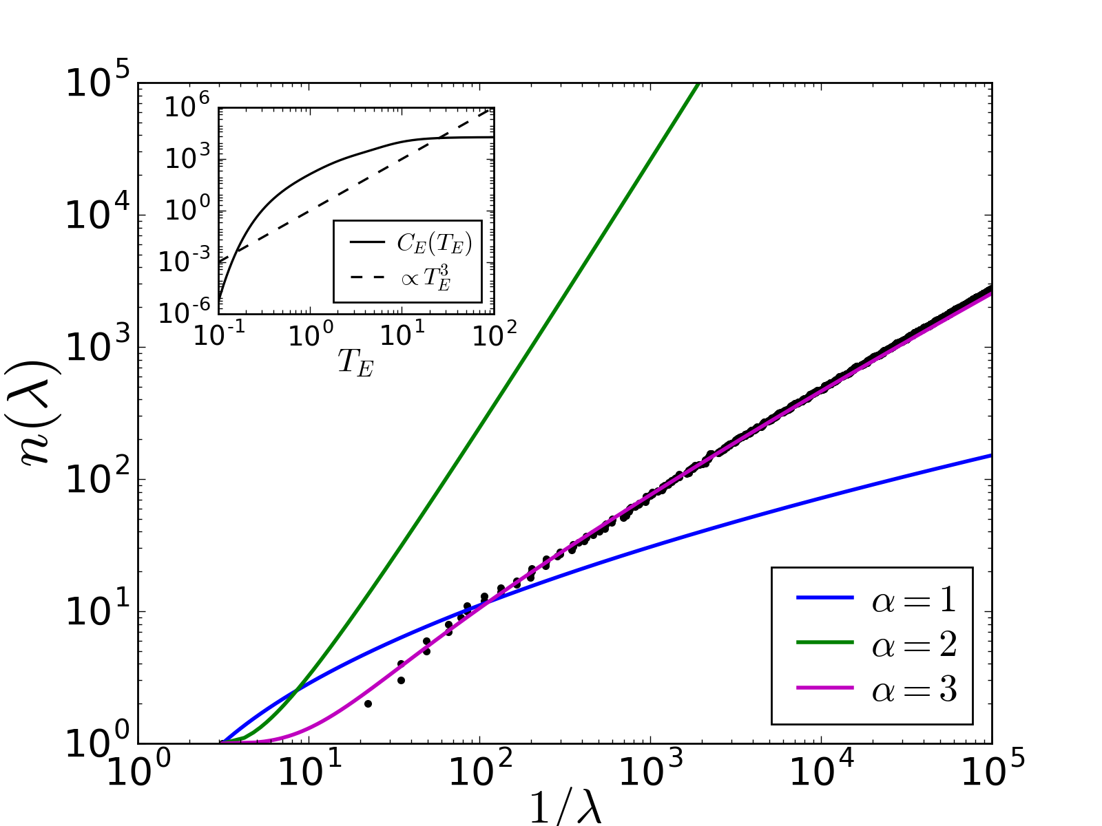
Figure 1: (color online) Cumulative distribution function $n(\lambda)$ of the RDM eigenvalues in relativistic free scalar boson in two spatial dimensions. In numerical calculations, we discretized the field theory and took as the subregion $A$ a circle with a radius of $10$ discretized units. Lines indicate the analytic formula (8) for three different values of the exponent $\alpha$. We find a good agreement of the numerical data with the $\alpha=1$ formula. The inset shows the COE $C_{E}(T_{E})$ (solid line) in comparison with the expected low-$T_{E}$ scaling $C_{E}\propto T_{E}^{3}$ Nakaguchi and Nishioka (2016) (dashed line).

Building on the analytic expression of the Rényi EE obtained by Klebanov et al. Klebanov et al. (2012), Nakaguchi and Nishioka Nakaguchi and Nishioka (2016) have calculated the COE of relativistic massless free scalar boson . In two spatial dimensions, in particular, the COE has been shown to scale as $C_{E}\sim T_{E}^{3}$ at low $T_{E}$. Interestingly, this is different from the low-$T$ behavior of the physical heat capacity $C\sim T^{2}$, providing a counterexample to the correspondence between the two quantities.

An advantage of this system for testing the formula (8) is the availability of an efficient numerical technique for computing the RDM eigenvalues. Following Ref. Nakaguchi and Nishioka (2015), we discretize the field theory of scaler boson $\phi$ with the action

$$S=\int d^{2}xdt\left[(\partial_{t}\phi)^{2}-(\nabla\phi)^{2}\right],$$ (9)

and calculate the RDM eigenvalues by taking as a subregion $A$ a circle centering at the origin. Further technical details of the numerical calculation are described in Appendix B.

Figure 1 presents the cumulative distribution function $n(\lambda)$ and the COE $C_{E}(T_{E})$ (inset) calculated numerically. It is clear that the data of $n(\lambda)$ agree well with the analytic formula with $\alpha=3$ as expected. In contrast, the data of $C_{E}(T_{E})$ plotted in logarithmic scales show a significant variation of slope; estimation of $\alpha$ through the fitting with the form $C_{E}\sim T_{E}^{\alpha}$ would crucially depend on the range of $T_{E}$ used for the fitting. These results indicate an advantage of $n(\lambda)$ over the COE $C_{E}(T_{E})$ in determining the exponent $\alpha$. This advantage results from a sensitive dependence of the formula (8) on $\alpha$.

III.2 Half-filled Landau level

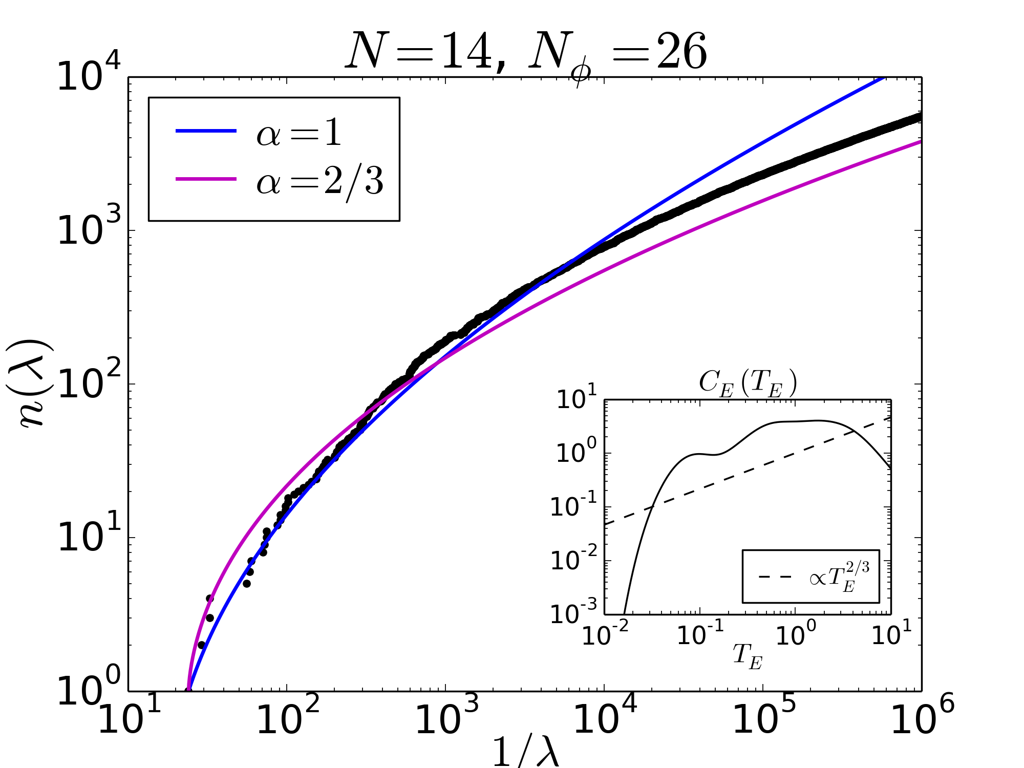
Figure 2: (color online) Cumulative distribution function $n(\lambda)$ of the RDM eigenvalues for the ground state of the half-filled Landau level (dots), in comparison with the analytic formula (8) for $\alpha=2/3$ and $\alpha=1$ (lines). The left and right panels correspond to the Fermi sea case ($N_{\phi}=2N-2$) and the particle-hole symmetric case ($N_{\phi}=2N-1$), respectively, where $N$ is set to $14$. In plotting the analytical formula, the numerically obtained value of $\lambda_{\mathrm{max}}$ is used. The insets show the COE $C_{E}(T_{E})$ (solid line) in comparison with the power-law behavior $C_{E}\propto T_{E}^{2/3}$ (dashed line).

As a more nontrivial application of our formula (8), we consider a quantum Hall system at the filling factor $\nu=1/2$ (half-filled Landau level). For this system, HLR formulated an effective field theory in which composite fermions forms a Fermi sea and interact via a Chern-Simons gauge field Halperin et al. (1993). Gauge fluctuations in this theory were shown to make a singular contribution to a heat capacity Halperin et al. (1993); Kim and Lee (1996). In particular, when the bare interaction between fermions is short-range, the heat capacity was predicted to scale as $C\sim T^{2/3}$, indicating a non-Fermi-liquid behavior. However, this prediction has not been verified numerically as a large number of low-lying eigenenergies are required to obtain a low-temperature behavior of the heat capacity. Recently, there have been very active studies on the role of particle-hole symmetry in this system. The HLR theory does not satisfy this symmetry, and an alternative description in terms of Dirac composite fermions consistent with this symmetry has been developed Son (2015); Wang and Senthil (2016a, b); Geraedts et al. (2016); Levin and Son (2017). In this description, Dirac composite fermions have a Fermi surface and interact via a gauge field without a Chern-Simons term. While the heat capacity has not been calculated in the Dirac scenario, the gauge field coupled with a Fermi surface is still expected to make a significant contribution.

Concerning entanglement properties, the $n=2$ Rényi EE has recently been calculated for trial wave functions of the half-filled Landau level, and a multiplicative logarithmic correction to the boundary law, which indicates a hidden Fermi surface, has been verified Shao et al. (2015); Mishmash and Motrunich (2016). However, the Rényi EE for fixed $n$ could not reveal a non-Fermi-liquid nature of the system. This motivates us to investigate the COE and the distribution of RDM eigenvalues in this system.

We performed exact diagonalization calculation for interacting $N$ spinless fermions in the lowest Landau level on a spherical geometry Haldane (1983). In this geometry, a magnetic monopole of charge $N_{\phi}$ in units of the flux quantum $h/e$ is placed at the center. We assume a repulsive short-range interaction $V(\bm{r})=-\nabla^{2}\delta(\bm{r})$ between fermions; this interaction is equivalent to the Haldane’s pseudopotential for $\nu=1/3$ Laughlin state Haldane (1983); Trugman and Kivelson (1985) while we here focus on the filling $\nu=1/2$. A Fermi sea of composite fermions corresponds to a set of $(N,N_{\phi})$ satisfying $N_{\phi}=2N-2$ Rezayi and Read (1994) whereas the particle-hole symmetric state (with a possible Dirac nature) is consistent with those satisfying $N_{\phi}=2N-1$ Son (2015). We investigate both types of states in numerical calculations; in the thermodynamic limit, they both correspond to the filling factor $\nu=1/2$. The ground state is $(2L+1)$-fold degenerate if it has a total angular momentum of magnitude $L>0$; in such a case, we took the ground state in the $L_{z}=0$ sector for the computation of the RDM, where $L_{z}$ is the $z$-component of the total angular momentum. From such a ground state, we calculated the eigenvalues of the RDM associated with the real-space cut into two hemispheres Sterdyniak et al. (2012); Dubail et al. (2012a).

Figures 2 and 3 present the cumulative distribution function $n(\lambda)$ and the COE $C_{E}(T_{E})$ (inset of Fig. 2) obtained in this way. In Fig. 2, we compare the numerical data of $n(\lambda)$ for $N=14$ with the analytic formulae with $\alpha=2/3$ and $\alpha=1$. The numerical data clearly show a better agreement with the $\alpha=2/3$ formula than with the $\alpha=1$ one, in both the Fermi sea case ($N_{\phi}=2N-2$) and the particle-hole symmetric case ($N_{\phi}=2N-1$). The data of $C_{E}(T_{E})$ plotted in logarithmic scales again show a variation of slope although a rough agreement with $\alpha=2/3$ is found for $10^{-1}\lesssim T_{E}\lesssim 10^{0}$. We furthermore compare the results for different $N$ in Fig. 3. One can see that the data of $n(\lambda)$ tend to approach the analytic formula with $\alpha=2/3$ with increasing $N$ although a marked deviation from the formula is found for $(N,N_{\phi})=(12,22)$. We infer that this deviation originates primarily from the spatial inhomogeneity of the fermion density around the boundary of the subregion $A$. When the ground state has a nonzero magnitude of the angular momentum $L>0$, the $L_{z}=0$ state used in our calculations can exhibit an inhomogeneous density that depends on the azimuthal angle $\theta$ (but not on the polar angle $\varphi$ because of the axial symmetry), as displayed in Fig. 4. The ground states for $(N,N_{\phi})=(12,22)$ and $(13,24)$ in the Fermi sea case have comparatively large $L$, and, as seen in the figure, show appreciable deviations of the density from the average value at the boundary of $A$ ($\theta=\pi/2$, the equator of the sphere). Therefore, these states can exhibit large finite-size effects; owing to their non-universal nature, such effects are prominent only for $(N,N_{\phi})=(12,22)$ in Fig. 3. In the particle-hole symmetric case (Fig. 4, right), because of a unique antisymmetric behavior, the deviation of the density from the average value vanishes at the boundary of $A$, which may explain smaller finite-size effects than the Fermi sea case as seen in Fig. 3.

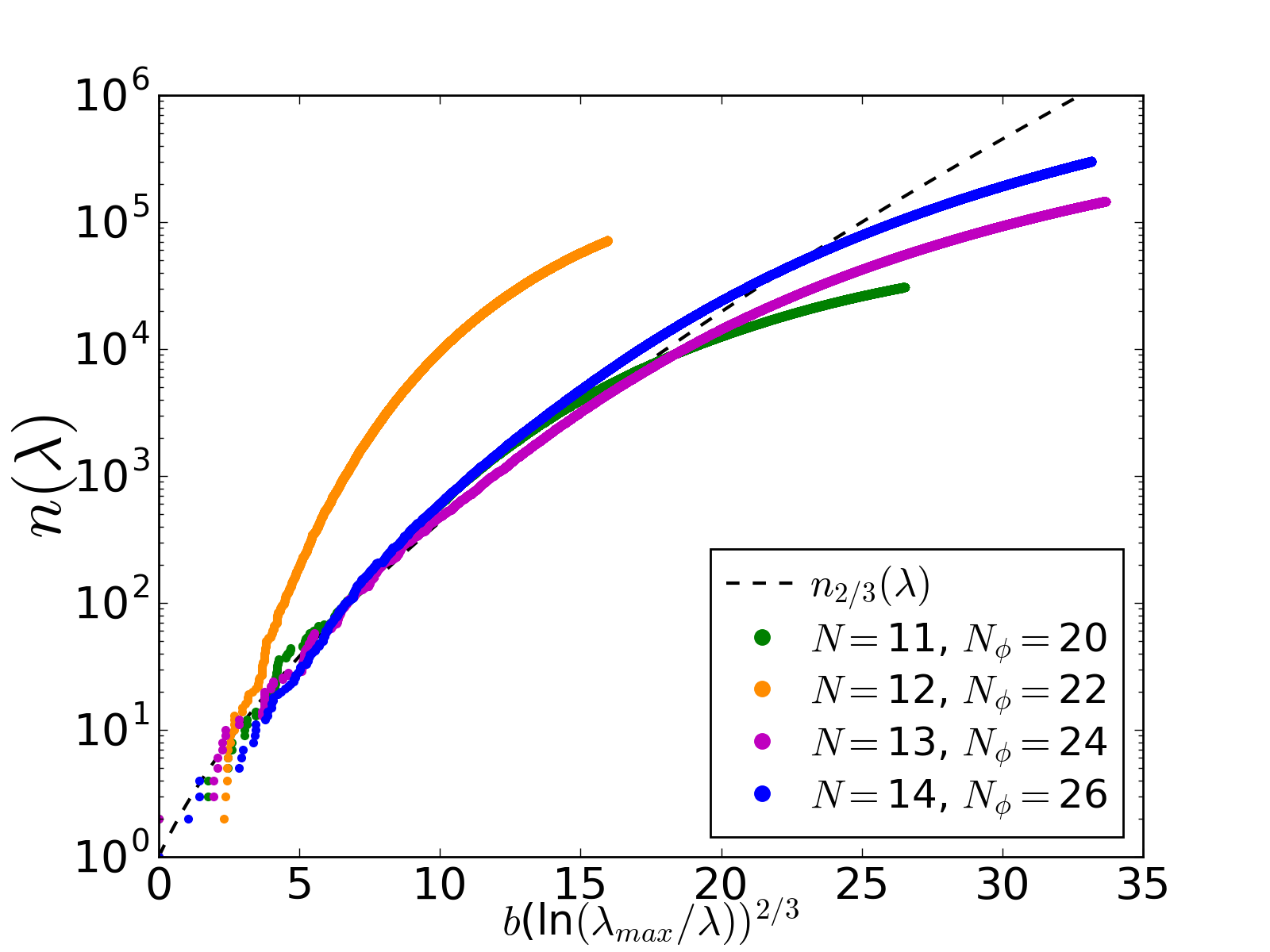
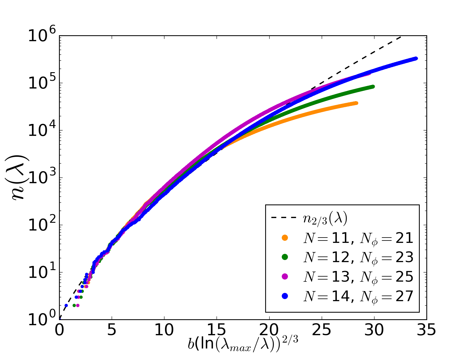
Figure 3: (color online) Cumulative distribution function $n(\lambda)$ for the ground state of the half-filled Landau level for different $N$. Numerical results (colored dots) are compared with the analytic formula (8) with $\alpha=2/3$ (dashed line). The left and right panels correspond to the Fermi sea case ($N_{\phi}=2N-2$) and the particle-hole symmetric case ($N_{\phi}=2N-1$), respectively.

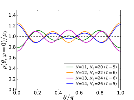
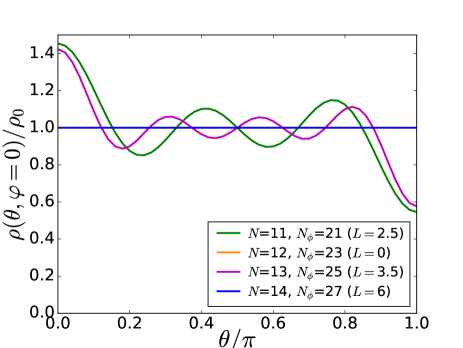
Figure 4: (color online) Density of fermions in the ground state of the half-filled Landau level in the cases examined in Fig. 3. The density $\rho(\theta,\varphi)$ is normalized by the average density $\rho_{0}=N/S$, where $S$ is the area of the sphere. The dashed line in the left panel indicates the case of homogeneous density as a guide for eyes. In the right panel, the data for $N=12$ and $14$ are overlapping.

IV Conclusions

In this paper, we have studied the COE $C_{E}(T_{E})$ and the cumulative distribution function $n(\lambda)$ of RDM eigenvalues in gapless systems. Assuming a power-law behavior $C_{E}\sim T_{E}^{\alpha}$ at low $T_{E}$, we have derived an analytic formula of $n(\lambda)$ as in Eq. (8). We have numerically tested the effectiveness of the formula in relativistic free scalar bosons in two spatial dimensions, and find that the distribution of RDM eigenvalues can detect the expected $\alpha=3$ scaling of the COE much more efficiently than the raw data of the COE. We have also calculated the distribution of RDM eigenvalues in the ground state of the half-filled Landau level with short-range interactions, and find a better agreement with the $\alpha=2/3$ formula than with the $\alpha=1$ one, which indicates a non-Fermi-liquid nature of the system. We have also found that our data tend to approach the $\alpha=2/3$ formula with increasing $N$. This suggests an intriguing possibility that the COE and the physical heat capacity show the same power-law behavior in this strongly interacting metallic state.

The correspondence between the ES and the physical energy spectrum has been known in gapped topological phases Kitaev and Preskill (2006); Li and Haldane (2008); Thomale et al. (2010); Yao and Qi (2010); Turner et al. (2010); Fidkowski (2010); Sterdyniak et al. (2012); Dubail et al. (2012a); Qi et al. (2012); Chandran et al. (2011); Dubail et al. (2012b); Swingle and Senthil (2012); Lundgren et al. (2013); Cano et al. (2015) and in some gapless systems Läuchli (2013); Metlitski and Grover (2011); Alba et al. (2013); Kolley et al. (2013). Our numerical result on the half-filled Landau level suggests that this correspondence also holds in a strongly interacting metallic state. It would be interesting to investigate whether this correspondence holds in other gapless systems with strong interactions. Calculation of the distribution of RDM eigenvalues would be useful for this purpose as the comparison with the analytical formula (8) allows us to efficiently probe the low-energy properties of the ES as demonstrated in this paper. This contrasts with the strategies of Refs. Läuchli (2013); Metlitski and Grover (2011); Alba et al. (2013); Kolley et al. (2013), where the ES was compared with the known tower structure of the bulk energy spectrum; the use of the distribution of RDM eigenvalues does not require such prior knowledge. While the general condition for the correspondence between the ES and the physical spectrum is not known, the deviation of the COE or the distribution function from the $\alpha=1$ behavior can already signal a non-Fermi-liquid nature, as explained in Sec. I. A particularly interesting class of systems to apply this idea are critical spin liquids with a spinon Fermi surface as studied in Zhang et al. (2011); Grover et al. (2013), which are also considered to show a heat capacity scaling as $T^{2/3}$ similarly to the half-filled Landau level.

Appendix A $n_{\alpha}(\lambda)$ as a sum of hypergeometric function

When the exponent $\alpha$ of the COE is a rational number, the formula $n_{\alpha}(\lambda)$ for the cumulative distribution function in Eq. (8) can be written as a sum of the hypergeometric functions. In this appendix, we present explicit forms of such expressions.

The hypergeometric function is defined as

$${}_{p}F_{q}(\{a_{1},\ldots,a_{p}\};\{b_{1},\ldots,b_{q}\};x)=\sum_{k=0}^{\infty}\frac{(a_{1})_{k}\cdots(a_{p})_{k}}{(b_{1})_{k}\cdots(b_{q})_{k}}\frac{x^{k}}{k!},$$ (10)

where rising factorial $(a_{i})_{k}$ is defined as $(a_{i})_{k}:=a_{i}(a_{i}+1)\cdots(a_{i}+k-1)=\Gamma(a_{i}+k)/\Gamma(a_{i})$. When $\alpha$ equals an integer $m\in\mathbb{N}^{+}=\{1,2,\cdots\}$, one can show that Eq. (8) reduces to

$$n_{m}(\lambda)=_{0}\!\!F_{m}\left(\{\};\left\{\frac{1}{m},\ldots,\frac{m-1}{m},1\right\};\,\frac{x}{m^{m}}\right),$$ (11)

where $x=b\left(\ln(\lambda_{\mathrm{max}}/\lambda)\right)^{m}$. When $\alpha$ is not an integer but a rational number, $\alpha=p/q$ ($p$ and $q$ are coprime integers), we observe that Eq. (8) can be written as the sum of the hypergeometric functions ${}_{0}F_{M}(gx^{q})$ with $x=b\left(\ln(\lambda_{\mathrm{max}}/\lambda)\right)^{\alpha}$, where a rational number $g$ and an integer $M$ are determined from $p$ and $q$. For example, when $\alpha=2/3$ we obtain

$$n_{2/3}(\lambda)= ~{}_{0}F_{4}\left(\{\};\left\{\frac{1}{3},\frac{1}{2},\frac{2}{3},1\right\};\frac{x^{3}}{108}\right)$$

$$+ \frac{x}{\Gamma\left(\frac{5}{3}\right)}~{}_{0}F_{4}\left(\{\};\left\{\frac{2}{3},\frac{5}{6},\frac{4}{3},\frac{4}{3}\right\};\frac{x^{3}}{108}\right)$$

$$+ \frac{3x^{2}}{8\Gamma\left(\frac{4}{3}\right)}~{}_{0}F_{4}\left(\{\};\left\{\frac{7}{6},\frac{4}{3},\frac{5}{3},\frac{5}{3}\right\};\frac{x^{3}}{108}\right),$$

where $x=b\left(\ln(\lambda_{\mathrm{max}}/\lambda)\right)^{2/3}$.

Appendix B Technical details on numerical calculations in relativistic free scalar bosons

In Sec. III.1, we calculated the eigenvalues of a RDM for the ground state of relativistic free scaler bosons in two spatial dimensions. This calculation was based on the method of Ref. Nakaguchi and Nishioka (2015), and we here describe some technical details for completeness.

The field-theory action in continuum is given by $S=\int d^{2}xdt[(\partial_{t}\phi)^{2}-(\nabla\phi)^{2}]$. We decompose this action in terms of the angular momentum $n$, and then discretize the radial direction into $N$ points labeled by $i\in\{1,\ldots,N\}$. Setting the lattice constant to unity, the resulting Hamiltonian is given by

$$H=\frac{1}{2}\sum_{n=-\infty}^{\infty}\left(\sum_{i=1}^{N}\pi_{n,i}^{2}+\sum_{i,j=1}^{N}\phi_{n,i}K^{i,j}_{n}\phi_{n.j}\right),$$

where $\phi_{n,i}$ and $\pi_{n,i}$ are the discretized scaler field and its conjugate field, respectively, for the angular momentum $n$ and the “site” $i$. The coefficients $K_{n}^{i,j}$ are given by $K_{n}^{1,1}=3/2+n^{2}$, $K_{n}^{i,i}=2+n^{2}/i^{2}\>\>(i\geq 2)$, $K_{n}^{i,i+1}=K_{n}^{i+1,i}=-(i+1/2)/\sqrt{i(i+1)}$, and $K_{n}^{i,j}=0$ (otherwise).

We take as a subregion $A$ a circle of radius $R$ centering at the origin ($0<R<N$). Since the theory is free (quadratic), the RDM of the ground state for the subregion $A$ can be written as a Gibbs state $\rho_{A}\propto\exp\left(-\sum_{k}\epsilon_{k}b_{k}^{\dagger}b_{k}\right)$, where $b_{k}^{\dagger}$ and $b_{k}$ are some bosonic creation and annihilation operators. The single-particle “entanglement energy” $\epsilon_{k}$ can be calculated from eigenvalues of the correlation matrix $C$ in the subregion $A$ Peschel (2003); Peschel and Eisler (2009); Casini and Huerta (2009). The correlation matrix $C$ is defined through the correlation functions in the ground state as $C=\sqrt{XP}$, where $X_{i,j}:=\otimes_{n}\langle\phi_{n,i}\phi_{n,j}\rangle_{GS}$ and $P_{i,j}:=\otimes_{n}\langle\pi_{n,i}\pi_{n,j}\rangle_{GS}$ $(i,j=1,\ldots,R)$. The eigenvalues of $C$, which we denote by $\xi_{k}$, are related with $\epsilon_{k}$ as $\frac{1}{2}\mathrm{coth}\left(\epsilon_{k}/2\right)=\xi_{k}$. From $\epsilon_{k}$, the many-body spectrum of $\rho_{A}$ and the distribution function $n(\lambda)$ are calculated.

For the data presented in Fig. 1, we set $N=40$ and $R=10$. Since the correlation matrix $C$ is block-diagonalized in terms of the angular momentum $n$, $\epsilon_{k}$’s can be calculated separately for different $n$. Since $\epsilon_{k}$ for large $|n|$ is generally small, we introduce a cutoff $n_{\mathrm{max}}$ for $n$ in numerical calculations. We checked that the results do not change when we increase $N$ or $n_{\mathrm{max}}$ while $R/N$ is fixed.

References

- Laflorencie (2016) Nicolas Laflorencie, “Quantum entanglement in condensed matter systems,” Physics Reports 646, 1 – 59 (2016), quantum entanglement in condensed matter systems.
- Amico et al. (2008) Luigi Amico, Rosario Fazio, Andreas Osterloh, and Vlatko Vedral, “Entanglement in many-body systems,” Rev. Mod. Phys. 80, 517–576 (2008).
- Srednicki (1993) Mark Srednicki, “Entropy and area,” Phys. Rev. Lett. 71, 666–669 (1993).
- Eisert et al. (2010) J. Eisert, M. Cramer, and M. B. Plenio, “Colloquium : Area laws for the entanglement entropy,” Rev. Mod. Phys. 82, 277–306 (2010).
- Holzhey et al. (1994) Christoph Holzhey, Finn Larsen, and Frank Wilczek, “Geometric and renormalized entropy in conformal field theory,” Nuclear Physics B 424, 443 – 467 (1994).
- Vidal et al. (2003) G. Vidal, J. I. Latorre, E. Rico, and A. Kitaev, “Entanglement in quantum critical phenomena,” Phys. Rev. Lett. 90, 227902 (2003).
- Calabrese and Cardy (2004) Pasquale Calabrese and John Cardy, “Entanglement entropy and quantum field theory,” Journal of Statistical Mechanics: Theory and Experiment 2004, P06002 (2004).
- Calabrese and Cardy (2009) Pasquale Calabrese and John Cardy, “Entanglement entropy and conformal field theory,” Journal of Physics A: Mathematical and Theoretical 42, 504005 (2009).
- Wolf (2006) Michael M. Wolf, “Violation of the entropic area law for fermions,” Phys. Rev. Lett. 96, 010404 (2006).
- Gioev and Klich (2006) Dimitri Gioev and Israel Klich, “Entanglement entropy of fermions in any dimension and the widom conjecture,” Phys. Rev. Lett. 96, 100503 (2006).
- Swingle (2010) Brian Swingle, “Entanglement entropy and the fermi surface,” Phys. Rev. Lett. 105, 050502 (2010).
- Swingle (2012) Brian Swingle, “Conformal field theory approach to fermi liquids and other highly entangled states,” Phys. Rev. B 86, 035116 (2012).
- Ding et al. (2012) Wenxin Ding, Alexander Seidel, and Kun Yang, “Entanglement entropy of fermi liquids via multidimensional bosonization,” Phys. Rev. X 2, 011012 (2012).
- McMinis and Tubman (2013) Jeremy McMinis and Norm M. Tubman, “Renyi entropy of the interacting fermi liquid,” Phys. Rev. B 87, 081108 (2013).
- Zhang et al. (2011) Yi Zhang, Tarun Grover, and Ashvin Vishwanath, “Entanglement entropy of critical spin liquids,” Phys. Rev. Lett. 107, 067202 (2011).
- Grover et al. (2013) Tarun Grover, Yi Zhang, and Ashvin Vishwanath, “Entanglement entropy as a portal to the physics of quantum spin liquids,” New Journal of Physics 15, 025002 (2013).
- Swingle and Senthil (2013) Brian Swingle and T. Senthil, “Universal crossovers between entanglement entropy and thermal entropy,” Phys. Rev. B 87, 045123 (2013).
- Shao et al. (2015) Junping Shao, Eun-Ah Kim, F. D. M. Haldane, and Edward H. Rezayi, “Entanglement entropy of the composite fermion non-fermi liquid state,” Phys. Rev. Lett. 114, 206402 (2015).
- Mishmash and Motrunich (2016) Ryan V. Mishmash and Olexei I. Motrunich, “Entanglement entropy of composite fermi liquid states on the lattice: In support of the widom formula,” Phys. Rev. B 94, 081110 (2016).
- Lai and Yang (2016) Hsin-Hua Lai and Kun Yang, “Probing critical surfaces in momentum space using real-space entanglement entropy: Bose versus fermi,” Phys. Rev. B 93, 121109 (2016).
- Ogawa et al. (2012) Noriaki Ogawa, Tadashi Takayanagi, and Tomonori Ugajin, “Holographic fermi surfaces and entanglement entropy,” Journal of High Energy Physics 2012, 125 (2012).
- Huijse et al. (2012) Liza Huijse, Subir Sachdev, and Brian Swingle, “Hidden fermi surfaces in compressible states of gauge-gravity duality,” Phys. Rev. B 85, 035121 (2012).
- Kitaev and Preskill (2006) Alexei Kitaev and John Preskill, “Topological entanglement entropy,” Phys. Rev. Lett. 96, 110404 (2006).
- Levin and Wen (2006) Michael Levin and Xiao-Gang Wen, “Detecting topological order in a ground state wave function,” Phys. Rev. Lett. 96, 110405 (2006).
- Hamma et al. (2005a) Alioscia Hamma, Radu Ionicioiu, and Paolo Zanardi, “Bipartite entanglement and entropic boundary law in lattice spin systems,” Phys. Rev. A 71, 022315 (2005a).
- Hamma et al. (2005b) Alioscia Hamma, Radu Ionicioiu, and Paolo Zanardi, “Ground state entanglement and geometric entropy in the kitaev model,” Physics Letters A 337, 22 – 28 (2005b).
- Metlitski et al. (2009) Max A. Metlitski, Carlos A. Fuertes, and Subir Sachdev, “Entanglement entropy in the model,” Phys. Rev. B 80, 115122 (2009).
- Hsu et al. (2009) Benjamin Hsu, Michael Mulligan, Eduardo Fradkin, and Eun-Ah Kim, “Universal entanglement entropy in two-dimensional conformal quantum critical points,” Phys. Rev. B 79, 115421 (2009).
- Stéphan et al. (2009) Jean-Marie Stéphan, Shunsuke Furukawa, Grégoire Misguich, and Vincent Pasquier, “Shannon and entanglement entropies of one- and two-dimensional critical wave functions,” Phys. Rev. B 80, 184421 (2009).
- Islam et al. (2015) Rajibul Islam, Ruichao Ma, Philipp M. Preiss, M. Eric Tai, Alexander Lukin, Matthew Rispoli, and Markus Greiner, “Measuring entanglement entropy in a quantum many-body system,” Nature 528, 77–83 (2015).
- Kaufman et al. (2016) Adam M. Kaufman, M. Eric Tai, Alexander Lukin, Matthew Rispoli, Robert Schittko, Philipp M. Preiss, and Markus Greiner, “Quantum thermalization through entanglement in an isolated many-body system,” Science 353, 794–800 (2016).
- Pichler et al. (2016) Hannes Pichler, Guanyu Zhu, Alireza Seif, Peter Zoller, and Mohammad Hafezi, “Measurement protocol for the entanglement spectrum of cold atoms,” Phys. Rev. X 6, 041033 (2016).
- Li and Haldane (2008) Hui Li and F. D. M. Haldane, “Entanglement spectrum as a generalization of entanglement entropy: Identification of topological order in non-abelian fractional quantum hall effect states,” Phys. Rev. Lett. 101, 010504 (2008).
- Thomale et al. (2010) R. Thomale, A. Sterdyniak, N. Regnault, and B. Andrei Bernevig, “Entanglement gap and a new principle of adiabatic continuity,” Phys. Rev. Lett. 104, 180502 (2010).
- Yao and Qi (2010) Hong Yao and Xiao-Liang Qi, “Entanglement entropy and entanglement spectrum of the kitaev model,” Phys. Rev. Lett. 105, 080501 (2010).
- Turner et al. (2010) Ari M. Turner, Yi Zhang, and Ashvin Vishwanath, “Entanglement and inversion symmetry in topological insulators,” Phys. Rev. B 82, 241102 (2010).
- Fidkowski (2010) Lukasz Fidkowski, “Entanglement spectrum of topological insulators and superconductors,” Phys. Rev. Lett. 104, 130502 (2010).
- Sterdyniak et al. (2012) A. Sterdyniak, A. Chandran, N. Regnault, B. A. Bernevig, and Parsa Bonderson, “Real-space entanglement spectrum of quantum hall states,” Phys. Rev. B 85, 125308 (2012).
- Dubail et al. (2012a) J. Dubail, N. Read, and E. H. Rezayi, “Real-space entanglement spectrum of quantum hall systems,” Phys. Rev. B 85, 115321 (2012a).
- Qi et al. (2012) Xiao-Liang Qi, Hosho Katsura, and Andreas W. W. Ludwig, “General relationship between the entanglement spectrum and the edge state spectrum of topological quantum states,” Phys. Rev. Lett. 108, 196402 (2012).
- Chandran et al. (2011) Anushya Chandran, M. Hermanns, N. Regnault, and B. Andrei Bernevig, “Bulk-edge correspondence in entanglement spectra,” Phys. Rev. B 84, 205136 (2011).
- Dubail et al. (2012b) J. Dubail, N. Read, and E. H. Rezayi, “Edge-state inner products and real-space entanglement spectrum of trial quantum hall states,” Phys. Rev. B 86, 245310 (2012b).
- Swingle and Senthil (2012) Brian Swingle and T. Senthil, “Geometric proof of the equality between entanglement and edge spectra,” Phys. Rev. B 86, 045117 (2012).
- Lundgren et al. (2013) Rex Lundgren, Yohei Fuji, Shunsuke Furukawa, and Masaki Oshikawa, “Entanglement spectra between coupled tomonaga-luttinger liquids: Applications to ladder systems and topological phases,” Phys. Rev. B 88, 245137 (2013).
- Cano et al. (2015) Jennifer Cano, Taylor L. Hughes, and Michael Mulligan, “Interactions along an entanglement cut in abelian topological phases,” Phys. Rev. B 92, 075104 (2015).
- Chandran et al. (2014) Anushya Chandran, Vedika Khemani, and S. L. Sondhi, “How universal is the entanglement spectrum?” Phys. Rev. Lett. 113, 060501 (2014).
- Ho et al. (2015) Wen Wei Ho, Lukasz Cincio, Heidar Moradi, Davide Gaiotto, and Guifre Vidal, “Edge-entanglement spectrum correspondence in a nonchiral topological phase and kramers-wannier duality,” Phys. Rev. B 91, 125119 (2015).
- Läuchli (2013) Andreas M. Läuchli, “Operator content of real-space entanglement spectra at conformal critical points,” (2013), arXiv:1303.0741 [cond-mat.stat-mech] .
- Metlitski and Grover (2011) Max A. Metlitski and Tarun Grover, arXiv: 1112.2215 (2011).
- Alba et al. (2013) Vincenzo Alba, Masudul Haque, and Andreas M. Läuchli, “Entanglement spectrum of the two-dimensional bose-hubbard model,” Phys. Rev. Lett. 110, 260403 (2013).
- Kolley et al. (2013) F. Kolley, S. Depenbrock, I. P. McCulloch, U. Schollwöck, and V. Alba, “Entanglement spectroscopy of su(2)-broken phases in two dimensions,” Phys. Rev. B 88, 144426 (2013).
- Chen and Fradkin (2013) Xiao Chen and Eduardo Fradkin, “Quantum entanglement and thermal reduced density matrices in fermion and spin systems on ladders,” Journal of Statistical Mechanics: Theory and Experiment 2013, P08013 (2013).
- Schliemann (2011) John Schliemann, “Entanglement spectrum and entanglement thermodynamics of quantum hall bilayers at ,” Phys. Rev. B 83, 115322 (2011).
- Nakaguchi and Nishioka (2016) Yuki Nakaguchi and Tatsuma Nishioka, “A holographic proof of rényi entropic inequalities,” Journal of High Energy Physics 2016, 129 (2016).
- not (2017) This can be seen by following the logic of Sec. II inversely from Eq. (4).
- Affleck (1986) Ian Affleck, “Universal term in the free energy at a critical point and the conformal anomaly,” Phys. Rev. Lett. 56, 746–748 (1986).
- Calabrese and Lefevre (2008) Pasquale Calabrese and Alexandre Lefevre, “Entanglement spectrum in one-dimensional systems,” Phys. Rev. A 78, 032329 (2008).
- Halperin et al. (1993) B. I. Halperin, Patrick A. Lee, and Nicholas Read, “Theory of the half-filled landau level,” Phys. Rev. B 47, 7312–7343 (1993).
- Barkeshli et al. (2015) Maissam Barkeshli, Michael Mulligan, and Matthew P. A. Fisher, “Particle-hole symmetry and the composite fermi liquid,” Phys. Rev. B 92, 165125 (2015).
- Murthy and Shankar (2016) Ganpathy Murthy and R. Shankar, “,” Phys. Rev. B 93, 085405 (2016).
- Son (2015) Dam Thanh Son, “Is the composite fermion a dirac particle?” Phys. Rev. X 5, 031027 (2015).
- Wang and Senthil (2016a) Chong Wang and T. Senthil, “Half-filled landau level, topological insulator surfaces, and three-dimensional quantum spin liquids,” Phys. Rev. B 93, 085110 (2016a).
- Wang and Senthil (2016b) Chong Wang and T. Senthil, “Composite fermi liquids in the lowest landau level,” Phys. Rev. B 94, 245107 (2016b).
- Geraedts et al. (2016) Scott D. Geraedts, Michael P. Zaletel, Roger S. K. Mong, Max A. Metlitski, Ashvin Vishwanath, and Olexei I. Motrunich, “The half-filled landau level: The case for dirac composite fermions,” Science 352, 197–201 (2016), http://science.sciencemag.org/content/352/6282/197.full.pdf .
- Levin and Son (2017) Michael Levin and Dam Thanh Son, “Particle-hole symmetry and electromagnetic response of a half-filled landau level,” Phys. Rev. B 95, 125120 (2017).
- Wang et al. (2017) Chong Wang, Nigel R. Cooper, Bertrand I. Halperin, and Ady Stern, “Particle-hole symmetry in the fermion-chern-simons and dirac descriptions of a half-filled landau level,” Phys. Rev. X 7, 031029 (2017).
- Kim and Lee (1996) Yong Baek Kim and Patrick A. Lee, “Specific heat and validity of the quasiparticle approximation in the half-filled landau level,” Phys. Rev. B 54, 2715–2717 (1996).
- Klebanov et al. (2012) Igor R. Klebanov, Silviu S. Pufu, Subir Sachdev, and Benjamin R. Safdi, “Rényi entropies for free field theories,” Journal of High Energy Physics 2012, 74 (2012).
- Nakaguchi and Nishioka (2015) Yuki Nakaguchi and Tatsuma Nishioka, “Entanglement entropy of annulus in three dimensions,” Journal of High Energy Physics 2015, 72 (2015).
- Haldane (1983) F. D. M. Haldane, “Fractional quantization of the hall effect: A hierarchy of incompressible quantum fluid states,” Phys. Rev. Lett. 51, 605–608 (1983).
- Trugman and Kivelson (1985) S. A. Trugman and S. Kivelson, “Exact results for the fractional quantum hall effect with general interactions,” Phys. Rev. B 31, 5280–5284 (1985).
- Rezayi and Read (1994) E. Rezayi and N. Read, “Fermi-liquid-like state in a half-filled landau level,” Phys. Rev. Lett. 72, 900–903 (1994).
- Peschel (2003) Ingo Peschel, “Calculation of reduced density matrices from correlation functions,” Journal of Physics A: Mathematical and General 36, L205 (2003).
- Peschel and Eisler (2009) Ingo Peschel and Viktor Eisler, “Reduced density matrices and entanglement entropy in free lattice models,” Journal of Physics A: Mathematical and Theoretical 42, 504003 (2009).
- Casini and Huerta (2009) H Casini and M Huerta, “Entanglement entropy in free quantum field theory,” Journal of Physics A: Mathematical and Theoretical 42, 504007 (2009).