Participation ratio for constraint-driven condensation with superextensive mass

Abstract

Broadly distributed random variables with a power-law distribution $f(m)\sim m^{-(1+\alpha)}$ are known to generate condensation effects, in the sense that, when the exponent $\alpha$ lies in a certain interval, the largest variable in a sum of $N$ (independent and identically distributed) terms is for large $N$ of the same order as the sum itself. In particular, when the distribution has infinite mean ($0<\alpha<1$) one finds unconstrained condensation, whereas for $\alpha>1$ constrained condensation takes places fixing the total mass to a large enough value $M=\sum_{i=1}^{N}m_{i}>M_{c}$. In both cases, a standard indicator of the condensation phenomenon is the participation ratio $Y_{k}=\langle\sum_{i}m_{i}^{k}/(\sum_{i}m_{i})^{k}\rangle$ ($k>1$), which takes a finite value for $N\to\infty$ when condensation occurs. To better understand the connection between constrained and unconstrained condensation, we study here the situation when the total mass is fixed to a superextensive value $M\sim N^{1+\delta}$ ($\delta>0$), hence interpolating between the unconstrained condensation case (where the typical value of the total mass scales as $M\sim N^{1/\alpha}$ for $\alpha<1$) and the extensive constrained mass. In particular we show that for exponents $\alpha<1$ a condensate phase for values $\delta>\delta_{c}=1/\alpha-1$ is separated from a homogeneous phase at $\delta<\delta_{c}$ from a transition line, $\delta=\delta_{c}$, where a weak condensation phenomenon takes place. We focus on the evaluation of the participation ratio as a generic indicator of condensation, also recalling or presenting results in the standard cases of unconstrained mass and of fixed extensive mass.

I Introduction

In the context of the sum of a large number of positive random variables, an interesting phenomenon occurs when a single variable carries a finite fraction of the sum SEM17 . Such a phenomenon has been put forward for instance in the context of the glass transition MPV87 ; Bouchaud97 . In the framework of particle or mass transport models BBJ97 ; MKB98 ; GSS03 ; MEZ05 ; EMZ06 ; EH05 ; S08-leshouches ; HMS09 ; WCBE14 ; EW14 , where the sum of the random variables is fixed to a constant value due to a conservation law of the underlying dynamics, this phenomenon has been called “condensation”. This condensation phenomenon has since then been reported in different contexts like in extreme value statistics EM08 , and in the sample variance of exponentially distributed random variables as well as for conditioned random-walks SEM14 ; SEM14b ; SEM17 . A similar mechanism is also at the basis of the condensation observed in the non-equilibrium dynamics of non-interacting field-theoretical models ZCG14 ; CGP15 ; Z15 ; CSZ17 . A more general type of condensation, induced by interaction, has also been put forward EHM06 , but in the following we shall focus on cases without interaction, apart from a possible constraint on the total mass.

As mentioned above, standard condensation results from the presence of a constraint fixing the sum of the random variables to a given value. However, the fact that a single random variable carries a finite fraction of the sum is also observed for fat-tailed random variables with infinite mean —a phenomenon sometimes called the Noah effect MW68 ; Magd08 . The goal of the present paper is to present a comparative study of these two scenarios, that we shall respectively denote as constrained condensation and unconstrained condensation. Note that the term ’condensation’ is usually used in the literature to describe the constrained case, but we shall extend its use to the unconstrained case, to emphasize possible analogies between the two scenarios. Considering the set of $N$ random variables $m_{i}$ with joint distribution $P(m_{1},\ldots,m_{N})$, unconstrained condensation takes place when the sum $M=\sum_{i=1}^{N}m_{i}$, in the limit $N\rightarrow\infty$, is dominated by few terms, i.e., a number of terms of order $\mathcal{O}(1)$. This happens for instance to the sum of $N$ independent and identically distributed (iid) Levy-type random variables, with probability density $f(m)$ such that $f(m)\approx A/m^{1+\alpha}$ when $m\to\infty$, with an exponent $0<\alpha<1$. This unconstrained condensation effect (sometimes also referred to as ’localization’ Bouchaud03 depending on the context) is often characterized by the participation ratio $Y_{k}$ Bouchaud97 ; Derrida97 , defined as

$$Y_{k}=\left<\frac{\sum_{i=1}^{N}m_{i}^{k}}{\left(\sum_{i=1}^{N}m_{i}\right)^{k}}\right>,$$ (1)

where $k>1$ is a real number, and where the brackets indicate an average over the $m_{i}$’s. For broadly distributed random variables it can be shown, with the calculation presented in Derrida97 and briefly recalled here in Sec. II, that there is a critical value $\alpha_{c}=1$ for the exponent of the power-law distribution such that for $\alpha>1$ the asymptotic value of the participation ratio is zero, $\lim_{N\rightarrow\infty}Y_{k}=0$, whereas for a broad enough tail, $0<\alpha<1$, one has $\lim_{N\rightarrow\infty}Y_{k}>0$ for any value $k>1$. The average in Eq. (1) is computed with respect to the probability distribution $P(m_{1},\ldots,m_{N})=\prod_{i=1}^{N}f(m_{i})$. The participation ratio is therefore the ‘order parameter’ for condensation in the sum of random variables. It is in fact easy to see from Eq. (1) that when all the random variables contribute ‘democratically’ to the sum, namely when each of them is of order $m_{i}\sim 1/N$, then the asymptotic behaviour of the participation ratio is $Y_{k}\sim 1/N^{k-1}$, which goes to zero when $N\to\infty$. In contrast, if the sum is dominated by few terms of order $m_{i}\sim N$, asymptotically one has $Y_{k}\sim 1$.

As a physical example, the relevance of participation ratios to unveil unconstrained condensation in the sum of broadly distributed random variables was also shown for the condensation in phase space associated to the glass transition in the Random Energy Model (REM) Derrida97 ; Bouchaud97 . The REM is a system with $2^{N}$ configurations, where each configuration $i$ has the Boltzmann weight $e^{-\beta E_{i}}$, and the energies $E_{i}$ are iid random variables, usually assumed to have a Gaussian distribution with a variance proportional to $N$. The random variables with respect to which the glass phase corresponds to a condensed phase are the probabilities $z_{i}(\beta)=e^{-\beta E_{i}}$ of the different configurations. The corresponding participation ratio takes the same form as Eq. (1), simply replacing $m_{i}$ by $z_{i}(\beta)$. It has been shown Derrida97 ; Bouchaud97 that for values of the inverse temperature $\beta>\beta_{c}$, where $\beta_{c}$ is the critical value of the glass transition, the value of the sum $\mathcal{Z}=\sum_{i=1}^{2^{N}}z_{i}(\beta)$ is dominated in the limit $N\rightarrow\infty$ by $\mathcal{O}(1)$ terms: in this case the asymptotic value of $Y_{k}$ is finite. In particular one can prove that for an inverse temperature $\beta>\beta_{c}$ the participation ratio of the REM has precisely the same form as for the sum of iid Levy random variables $m_{i}$ with distribution $p(m_{i})=m_{i}^{1+\beta_{c}/\beta}$ (the exponent $\alpha=\beta_{c}/\beta$ is thus proportional to temperature).

In the above cases, with iid random variables, unconstrained condensation occurs for $\alpha<1$, that is when the first moment of the power-law distribution is infinite. The situation is different, though, when one considers power-law distributed random variables with a fixed total sum $M=\sum_{i=1}^{N}m_{i}$, a case which we refer to as constraint-driven condensation, or simply constrained condensation. Such a phenomenon, which is also related to the large of heavy-tailed sums (see, e.g., MN98 ), is found for instance in the stationary distribution of the discrete Zero Range Process and its continuous variables generalization MEZ05 ; EMZ06 ; S08-leshouches . The latter is represented by a lattice with $N$ sites, each carrying a continuous mass $m_{i}$, endowed with some total-mass conserving dynamical rules. For this model the stationary distribution is:

$$P(m_{1},\ldots,m_{N}|\rho)=\frac{1}{\mathcal{Z}_{N}(\rho)}\prod_{i=1}^{N}f(m_{i})~{}\delta\left[\rho N-\sum_{i=1}^{N}m_{i}\right],$$ (2)

where $\rho$ is the average density fixed by the initial total mass $M=\rho N$, and where

$$\mathcal{Z}_{N}(\rho)=\int_{0}^{\infty}dm_{1}\ldots dm_{N}~{}\prod_{i=1}^{N}f(m_{i})~{}\delta\left[\rho N-\sum_{i=1}^{N}m_{i}\right].$$ (3)

is a normalization constant (or partition function). In mass transport models the shape of the distribution $f(m_{i})$ depends on the dynamical rules, and has typically a power-law tail,

$$f_{\alpha}(m)\approx\frac{A}{m^{1+\alpha}}.$$ (4)

In MEZ05 ; EMZ06 ; S08-leshouches it has been shown that, in the presence of a constraint on the total value of the mass, constrained condensation never takes place for exponents of the local power-law distribution in the interval $0<\alpha<1$, while on the contrary when $\alpha>1$ there exists a critical value $\rho_{c}$ such that for $\rho>\rho_{c}$ the system is in the condensed phase. It thus turns out that constraining the random variables to have a fixed sum deeply modifies their statistical properties in this case —while naive intuition based on elementary statistical physics like the equivalence of ensembles may suggest that fixing the sum may not make an important difference. It is also worth emphasizing a significant difference between constrained and unconstrained condensation. In the unconstrained case, a few variables carry a finite fraction of the sum, while in the constrained case, only a single variable takes a macroscopic fraction of the sum (note that the situation may be different, though, in the presence of correlations between the variables EHM06 ). We thus see that the ’condensation’ phenomenon we define here as a non-vanishing value of the participation ratio in the infinite $N$ limit is a weak notion of condensation, which is more general than the standard condensation reported in the constrained case. In particular, this weak condensation effect does not imply the existence of a proper condensate, that is a ’bump’ in the tail of the marginal distribution $p(m)$ with a vanishing relative width. The bump may have a non-vanishing relative width, or may even not exist, the distribution $p(m)$ being monotonously decreasing in this case (see EMZ06 for an exactly solvable example). When relevant, we shall emphasize this specific character of the condensation by using the term ’weak condensation’.

The goal of the present work is to understand the relation between these two cases, which differ only by the presence or absence of a constraint on the total mass, but yield opposite ranges of values of $\alpha$ for the existence of condensation. To better grasp the nature of this difference, we study here the case where the total mass is fixed to a superextensive value $M\sim N^{1+\delta}$, with $\delta>0$, thus extending some of the results presented in EMZ06 . The choice of a superextensive mass is motivated by the fact that in the unconstrained case, the total mass $M=\sum_{i=1}^{N}m_{i}$, being the sum of iid broadly distributed variables, typically scales superextensively, as $N^{1/\alpha}$, for $\alpha<1$. This suggests that the case of a superextensive fixed mass may be closer to the unconstrained case, and that the value $1+\delta=1/\alpha$ may play a specific role. This will be confirmed by the detailed calculations presented in Sec. IV. Yet, before dealing with the superextensive mass case, we will first recall in Sec. II how to compute the participation ratios in the case of unconstrained condensation, and present in Sec. III a simplified evaluation of the participation ratio in the case of constrained condensation with an extensive fixed mass.

II Unconstrained condensation

In the unconstrained case, where the masses are simply independent and identically distributed random variables with a broad distribution, the evaluation of the average participation ratio $Y_{k}$ is well-know and has been performed using different methods Bouchaud97 ; Derrida97 . We sketch here the derivation of $Y_{k}$ using the auxiliary integral method put forward in Derrida97 . Noting that

$$\frac{1}{\left(\sum_{i=1}^{N}m_{i}\right)^{k}}=\frac{1}{\Gamma(k)}\int_{0}^{\infty}dt\,t^{k-1}\,\exp\left(-t\sum_{i=1}^{N}m_{i}\right),$$ (5)

one obtains, using the property that the random variables $m_{i}$ are independent and identically distributed,

$$Y_{k}=\frac{N}{\Gamma(k)}\int_{0}^{\infty}dt\,t^{k-1}\langle e^{-tm}\rangle_{\alpha}^{N-1}\,\langle m^{k}e^{-tm}\rangle_{\alpha}$$ (6)

where the brackets $\langle\dots\rangle_{\alpha}$ indicate an average over a single variable $m$ with distribution given in Eq. (4); $\Gamma$ is the Euler Gamma function, defined as $\Gamma(k)=\int_{0}^{\infty}dt\,t^{k-1}e^{-t}$. For large $N$, the factor $\langle e^{-tm}\rangle_{\alpha}^{N-1}$ in Eq. (6) takes very small values except if $t$ is small, in which case $\langle e^{-tm}\rangle_{\alpha}$ is close to $1$. Using a simple change of variable, one finds for $0<\alpha<1$ Derrida97

$$1-\langle e^{-tm}\rangle_{\alpha}\approx a\,t^{\alpha}\qquad(t\to 0)$$ (7)

with $a=A\Gamma(1-\alpha)/\alpha$, so that for $N\to\infty$,

$$\langle e^{-tm}\rangle_{\alpha}^{N-1}\approx e^{-Nat^{\alpha}},$$ (8)

again for small $t$. In a similar way, one also obtains for $k>\alpha$ Derrida97

$$\langle m^{k}e^{-tm}\rangle_{\alpha}\approx A\Gamma(k-\alpha)\,t^{-(k-\alpha)}\qquad(t\to 0).$$ (9)

One thus has for large $N$

$$Y_{k}\approx\frac{NA\Gamma(k-\alpha)}{\Gamma(k)}\int_{0}^{\infty}dt\,t^{\alpha-1}\,e^{-Nat^{\alpha}}$$ (10)

Using now the change of variable $v=Nat^{\alpha}$, the last integral can be expressed in terms of the Gamma function, eventually leading, in the limit $N\to\infty$, to Bouchaud97 ; Derrida97 ,

$$Y_{k}=\frac{\Gamma(k-\alpha)}{\Gamma(k)\Gamma(1-\alpha)}\qquad(0<\alpha<1).$$ (11)

The participation ratio $Y_{k}$ is thus non-zero for $0<\alpha<1$, and goes to zero linearly when $\alpha\to 1$. A similar calculation in the case $\alpha>1$ yields $Y_{k}=0$ in the limit $N\to\infty$. Hence condensation occurs for $0<\alpha<1$ in the unconstrained case. As we shall see below, the opposite situation occurs in the constrained case.

III Constrained condensation

We now turn to the computation of the participation ratio $Y_{k}$ when the total mass in the system is constrained to have the extensive value $M=\rho N$, as a function of the exponent $\alpha$ and of the density $\rho$. Evaluating $Y_{k}$ as defined in Eq. (1) by averaging over the constrained probability distribution given in Eq. (2), the denominator is a constant and can be factored out of the average, yielding the simple result:

$$Y_{k}=\frac{1}{\rho^{k}N^{k-1}}\langle m^{k}\rangle=\frac{1}{\rho^{k}N^{k-1}}\int_{0}^{\infty}dm\,p(m)\,m^{k}$$ (12)

where the marginal distribution $p(m)$ is defined as

$$p(m)=f_{\alpha}(m)\,\frac{\mathcal{Z}_{N-1}\left(\rho-\frac{m}{N}\right)}{\mathcal{Z}_{N}(\rho)}.$$ (13)

Before discussing what happens for the range of exponents $\alpha$ where constrained condensation takes place, let us briefly explain why for $\alpha<1$ the presence of the constraint removes the condensation and the participation ratio in Eq. (12) vanish when $N\to\infty$.

III.1 $\alpha<1$: Absence of condensation

The first important issue to clarify is why the condensation taking place in the unconstrained case for values of the power-law exponent $\alpha$ [see Eq. (4)] in the range $0<\alpha<1$, then disappear when a constraint on the total mass value is applied. Why the constraint forces the system to stay in the homogeneous phase? To answer this question, it is useful to recall the expression of the partition function of the model in terms of its inverse Laplace transform:

$$\mathcal{Z}_{N}(\rho)=\frac{1}{2\pi i}\int_{s_{0}-i\infty}^{s_{0}+i\infty}ds\,\exp\{N[\log g_{\alpha}(s)+\rho s]\},$$ (14)

where

$$g_{\alpha}(s)=\int_{0}^{\infty}dmf_{\alpha}(m)e^{-sm}.$$ (15)

The values of $\rho$ in the homogeneous “fluid” phase are those for which the integral in Eq. (14) can be solved with the saddle-point method. In contrast, constrained condensation occurs for all values of $\rho$ such that the saddle-point equation

$$\rho=-\frac{g_{\alpha}^{\prime}(s)}{g_{\alpha}(s)}=\frac{\int_{0}^{\infty}dm\,f_{\alpha}(m)\,m\,e^{-sm}}{\int_{0}^{\infty}dm\,f_{\alpha}(m)\,e^{-sm}}=\frac{\langle m\,e^{-sm}\rangle_{\alpha}}{\langle e^{-sm}\rangle_{\alpha}},$$ (16)

admits no solution on the real axis. It can be checked by inspection that the function $h(s)=\log g_{\alpha}(s)+\rho s$ has a branch cut in the complex $s$ plane coinciding with the negative part of the real axis. The domain over which $s$ can be varied to look for a solution of the saddle point equation is the positive semiaxis $[0,+\infty[$. When increasing $s$, the function $\langle m\,e^{-sm}\rangle_{\alpha}/\langle e^{-sm}\rangle_{\alpha}$ monotonically decreases from its value $\langle m\rangle_{\alpha}$ reached for $s\to 0$ to $0$ for $s\to\infty$.

At this point we just need to recall that for $0<\alpha<1$ one has $\langle m\rangle_{\alpha}=\infty$. This means that it is possible to find a value $s^{*}$ which is a solution of Eq. (16) for any given value of $\rho$. Hence the integral representation of the partition function in Eq. (14) can always be treated in the saddle-point approximation, so that condensation, which is related to the breaking of the saddle-point approximation, never occurs. By exploiting the saddle-point approximation for the partition function it is then not difficult to compute explicitly the expression in Eq. (13), which reads

$$p(m)\sim\frac{e^{-s^{*}m}}{m^{1+\alpha}},$$ (17)

where $s^{*}<\infty$ is the solution of the saddle point equation. The vanishing of the participation ratio $Y_{k}$ then follows easily, according to its expression in Eq. (12), from the presence of the exponential cutoff in $p(m)$ [Eq. (17)]:

$$Y_{k}=\frac{\langle m^{k}\rangle}{\rho^{k}N^{k-1}},$$ (18)

where $\langle m^{k}\rangle=\int_{0}^{\infty}dm\,m^{k}\,p(m)$ is a function which does not depend on $N$ in the large $N$ limit, so that

$$\lim_{N\rightarrow\infty}\frac{\langle m^{k}\rangle}{\rho^{k}N^{k-1}}=0.$$ (19)

We have therefore seen that for any $\alpha<1$, if one constrains the system to have an extensive mass $M=\rho N$, the participation ratio vanishes in the thermodynamic limit: $\lim_{N\rightarrow\infty}Y_{k}=0$, as expected since no condensation occurs in this case.

III.2 $\alpha>1$: Homogeneous phase at low density ($\rho<\rho_{c}$)

As soon as the exponent $\alpha$ of the single-variable distribution is increased above $\alpha_{c}=1$, namely as soon as the first moment of the distribution $f_{\alpha}(m)$ becomes finite, a condensed phase appears at finite $\rho_{c}$. For any given value of $\alpha$ the critical density $\rho_{c}$ is the maximal density for which the saddle point equation Eq. (16) has a solution. As we have already noticed in the previous section, the maximum value which can be attained by the term on the right of Eq. (16) is $\langle m\rangle_{\alpha}$, so that for all values $\rho>\rho_{c}=\langle m\rangle_{\alpha}$ the saddle-point approximation breaks down and one has condensation MEZ05 ; EMZ06 . Nevertheless, for $\alpha>1$ and $\rho<\rho_{c}$ the system is still in the homogeneous phase and, similarly to what is done in the case $\alpha<1$, one can compute the marginal distribution $\rho(m)$ according to its definition in Eq. (13) by using the saddle-point approximation. The result is also in this case

$$p(m)\sim f_{\alpha}(m)\,e^{-m/m_{0}},$$ (20)

and we know from MEZ05 ; EMZ06 that the characteristic mass $m_{0}$ diverges when the density $\rho$ tends to $\rho_{c}$ as $m_{0}\sim(\rho-\rho_{c})^{-1}$ for $\alpha>2$ and as $m_{0}\sim(\rho-\rho_{c})^{-1/(\alpha-1)}$ for $1<\alpha<2$.

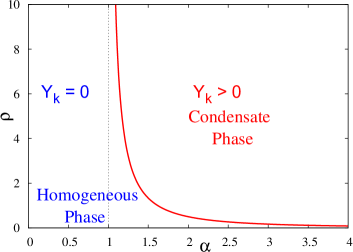
Figure 1: Phase diagram for the values of the participation rations in the ($\alpha$, $\rho$) plane in the presence of an extensive constraint on the total value of the mass $\sum_{i=1}^{N}m_{i}=\rho N$. The (red) continuous line marks the separation of the condensed phase ($\lim_{N\to\infty}Y_{k}>0$) and the homogeneous phase ($\lim_{N\to\infty}Y_{k}=0$). The vertical dotted (black) line marks the critical value $\alpha_{c}=1$ where the critical density $\rho_{c}$ for condensation diverges.

III.3 $\alpha>1$: Condensed phase at high density ($\rho>\rho_{c}$)

Let us now study what happens in the condensed phase. For $\alpha>1$ and $\rho>\rho_{c}$, one observes for large $N$ a coexistence between a homogeneous fluid phase carrying a total mass approximately equal to $N\rho_{c}$ and a condensate of mass $M_{\textrm{cond}}\approx(\rho-\rho_{c})N$. The marginal distribution $p(m)$ can be approximately written as EM08

$$p(m)\approx f(m)+p_{\textrm{cond}}(m,\rho,N)$$ (21)

where $p_{\textrm{cond}}(m,\rho,N)$ is the mass distribution of the condensate, normalized according to $\int_{0}^{\infty}p_{\textrm{cond}}(m,\rho,N)=1/N$ to account for the fact that the condensate is present on a single site. It has been shown MEZ05 ; EMZ06 that for $\alpha>2$, the distribution $p_{\textrm{cond}}(m,\rho,N)$ is Gaussian, with a width proportional to $N^{1/2}$. In other words, the condensate exhibits normal fluctuations. In contrast, for $1<\alpha<2$, the distribution $p_{\textrm{cond}}(m,\rho,N)$ has a broader, non-Gaussian shape, with a typical scale of fluctuation $\sim N^{1/\alpha}$ MEZ05 ; EMZ06 . For all values of $\alpha>1$, however, the relative fluctuations of $M_{\textrm{cond}}$ vanish in the large $N$ limit:

$$\frac{M_{\textrm{cond}}-\overline{M}_{\textrm{cond}}}{M_{\textrm{cond}}} \sim N^{-(\alpha-1)/\alpha}\qquad\,\textrm{if}\quad 1<\alpha<2$$ (22)

$$\sim N^{-1/2}\qquad\qquad\textrm{if}\quad\alpha>2$$

with $\overline{M}_{\textrm{cond}}=(\rho-\rho_{c})N$. Hence in order to compute the large $N$ behavior of moments of the distribution $p(m)$, one can further approximate $p(m)$ as

$$p(m)\approx f(m)+\frac{1}{N}\,\delta\left(\sum_{i=1}^{N}m_{i}-\overline{M}_{\textrm{cond}}\right)$$ (23)

Note that more accurate expressions of the distribution $p(m)$ can be found in EMZ06 .

From Eq. (23), the moment $\langle m^{k}\rangle$ is evaluated as

$$\langle m^{k}\rangle\approx\int_{0}^{\rho_{c}N}dm\,m^{k}f(m)+\frac{\overline{M}_{\textrm{cond}}^{k}}{N}.$$ (24)

The integral in Eq. (24), corresponding to the fluid phase contribution to the moment, has a different scaling with $N$ depending on the respective values of $k$ and $\alpha$. If $k<\alpha$, the integral converges to a finite limit when $N$ goes to infinity. On the contrary, when $k>\alpha$, the integral diverges with $N$ and scales as $N^{k-\alpha}$.

The participation ratio reads $Y_{k}=\langle m^{k}\rangle/(\rho^{k}N^{k-1})$, so that the contribution of the fluid phase to the participation ratio scales as $1/N^{k-1}$ for $k<\alpha$, and as $1/N^{\alpha-1}$ for $k>\alpha$; in both cases, this contribution vanishes for $N\to\infty$, when $k>1$ and $\alpha>1$. The remaining contribution, resulting from the condensate, simply leads to

$$Y_{k}=\left(\frac{\rho-\rho_{c}}{\rho}\right)^{k},$$ (25)

where we recall that $\rho>\rho_{c}$ in the condensed phase. Hence $Y_{k}$ goes to zero at the onset of condensation ($\rho\to\rho_{c}$), so that the transition can be thought as continuous if one considers the participation ratio as an order parameter. In the opposite limit $\rho\to\infty$, the participation ratio goes to $1$, indicating a full condensation.

A phase diagram in the $(\alpha,\rho)$-plane summarizing the results of this section for the case of constrained condensation with extensive mass is shown in Fig. 1.

IV Constraint to a superextensive total mass $M=\tilde{\rho}N^{1+\delta}$

As explained in the introduction, the unconstrained condensation occurs for $\alpha<1$, while the contraint-driven condensation occurs at $\alpha>1$ (and at high enough density). Given that the typical total mass in the unconstrained case is superextensive for $\alpha<1$, it is of interest to study condensation effects in the more general case of a fixed superextensive total mass $M=\tilde{\rho}N^{1+\delta}$, with $\delta>0$ and $\tilde{\rho}$ a parameter which generalizes the usual notion of density. The joint probability distribution $p(m_{1},\ldots,m_{N}|\tilde{\rho})$ reads in this case

$$p(m_{1},\ldots,m_{N}|\tilde{\rho})=\frac{1}{\mathcal{Z}_{N,\delta}(\tilde{\rho})}\prod_{i=1}^{N}f(m_{i})\delta\left[\sum_{i=1}^{N}m_{i}-\tilde{\rho}N^{1+\delta}\right],$$ (26)

where $\mathcal{Z}_{N,\delta}(\tilde{\rho})$ is a normalization factor [see Eq. (3)]. We wish to determine for which values of $\alpha$ and $\tilde{\rho}$ condensation occurs in this case, using as an order parameter for condensation the participation ratio $Y_{k}=N\langle m^{k}\rangle/M^{k}$, which reads in the present case as

$$Y_{k}=\frac{\langle m^{k}\rangle}{\tilde{\rho}^{k}N^{k-1+k\delta}}=\frac{1}{\rho^{k}N^{k-1+k\delta}}\int_{0}^{\infty}dm\,p(m)\,m^{k}.$$ (27)

The expression of the marginal distribution $p(m)$ in the case of the superextensive total mass is given below in Eq. (41).

In the following, we first use in Sec. IV.1 the integral representation of the partition function $\mathcal{Z}_{N}(\tilde{\rho})$ in order to get indications on the phase diagram in the $(\alpha,\delta)$ plane. This preliminary analysis will suggest the existence of a transition line, that will be confirmed in Sec. IV.2 to IV.4 by an explicit determination of the marginal distribution $p(m)$ and the participation ratio $Y_{k}$ respectively below, above and on the anticipated transition line.

IV.1 Preliminary analysis of the phase diagram

We start by expressing the partition function $\mathcal{Z}_{N,\delta}(\tilde{\rho})$ as an integral representation in terms of its inverse Laplace transform. The Laplace transform $\hat{\mathcal{Z}}_{N,\delta}(s)$ of $\mathcal{Z}_{N,\delta}(\tilde{\rho})$ is expressed as

$$\hat{\mathcal{Z}}_{N,\delta}(s)\equiv\int_{0}^{\infty}d\tilde{\rho}\,e^{-s\tilde{\rho}}\mathcal{Z}_{N,\delta}(\tilde{\rho})=\frac{1}{N^{1+\delta}}\,g_{\alpha}\left(\frac{s}{N^{1+\delta}}\right)^{N}$$ (28)

where $g_{\alpha}(s)$ is defined in Eq. (15). After a simple change of variable, the inverse Laplace representation of the partition function $\mathcal{Z}_{N}(\tilde{\rho})$ reads

$$\mathcal{Z}_{N,\delta}(\tilde{\rho})=\frac{1}{2\pi i}\int_{s_{0}-i\infty}^{s_{0}+i\infty}ds\,\exp\{N[\log g_{\alpha}(s)+\tilde{\rho}N^{\delta}s]\}.$$ (29)

The value of $s_{0}$, although arbitrary, can be conveniently chosen to be the saddle-point value of the argument of the exponential in Eq. (29), when a saddle-point $s_{0}>0$ exists (this is due to the presence of a branch-cut singularity on the negative real axis, as discussed in the previous section). When no saddle-point exists, the equivalence between canonical and grand-canonical ensemble breaks down, and condensation is expected to occur. A saddle-point of the integral in Eq. (29) should satisfy the following equation,

$$\tilde{\rho}N^{\delta}=-\frac{g_{\alpha}^{\prime}(s)}{g_{\alpha}(s)}=\frac{\langle m\,e^{-sm}\rangle_{\alpha}}{\langle e^{-sm}\rangle_{\alpha}}.$$ (30)

Note that this approach is heuristic, since the saddle-point should in principle not depend on $N$. However, the $N$-dependence is not a problem when testing the existence of a saddle-point. If it exists, the saddle-point evaluation of the integral then requires a change of variable for (some power of) $N$ to appear only as a global prefactor in the argument of the exponential.

For $\alpha>1$, we know from the results of section III that the saddle-point equation (30) has a solution only if $\tilde{\rho}N^{\delta}<\rho_{c}$. This condition is never satisfied for $\delta>0$ and $N\to\infty$, so that no saddle-point exists and condensation occurs for any value of $\tilde{\rho}>0$ when $\alpha>1$.

The situation is thus quite similar to the extensive mass case: there is a homogeneous phase carrying a total mass $N\rho_{c}$ which coexists with a superextensive condensate with a mass $M_{c}=\tilde{\rho}N^{1+\delta}-N\rho_{c}\approx\tilde{\rho}N^{1+\delta}$, so that the condensate carries a fraction of the total mass equal to one in the limit $N\to\infty$. It follows that the participation ratio $Y_{k}=1$ in this limit.

In contrast, for $\alpha<1$, the function $g_{\alpha}^{\prime}(s)/g_{\alpha}(s)$ spans the whole positive real axis, and the saddle-point equation (30) always has a solution $s_{0}(N)$, which goes to $0$ when $N\to\infty$. One then has to factor out the $N$-dependence through an appropriate change of variable, and to check whether a saddle-point evaluation of the integral can be made. For $s\to 0$, one has $g_{\alpha}^{\prime}(s)/g_{\alpha}(s)\approx a\alpha s^{\alpha-1}$, so that $s_{0}\sim N^{-\delta/(1-\alpha)}$. Using the change of variable $s=zN^{-\delta/(1-\alpha)}$ in the integral appearing in Eq. (30), the argument of the exponential can be rewritten as

$$N^{1-\alpha\delta/(1-\alpha)}(-az^{\alpha}+\tilde{\rho}z),\quad$$ (31)

with $a=A\,\Gamma(1-\alpha)/\alpha$, and where we have used the small-$s$ expansion $g_{\alpha}(s)\approx 1-as^{\alpha}$, valid for $0<\alpha<1$. The saddle-point evaluation of the integral is valid only if the $N$-dependent prefactor diverges, meaning that $1-\alpha\delta/(1-\alpha)>0$, or equivalently

$$\delta<\delta_{c}=\frac{1-\alpha}{\alpha}.$$ (32)

Hence for $\alpha<1$ and $\delta<\delta_{c}$, a saddle-point evaluation of the partition function is possible, and the equivalence between canonical and grand-canonical ensembles holds: the system is in the homogeneous phase, and no condensation occurs. For $\delta\geq\delta_{c}$, the saddle-point evaluation of the partition function is no longer possible, which suggests that the equivalence of ensembles breaks down. This is an indication that condensation may occur. We show through explicit calculations in Sec. IV.3 and Sec. IV.4 that condensation occurs when $\delta\geq\delta_{c}$, in the sense that the participation ratio $Y_{k}$ takes a nonzero value in the infinite $N$ limit.

Before proceeding to a detailed characterization of this condensation, let us briefly comment on the value of $\delta_{c}$. For $\delta=\delta_{c}$, the total mass in the system scales as $M\sim N^{1/\alpha}$, and this scaling precisely corresponds to the typical value of the total mass present in the unconstrained case (see section II), as already noticed in EMZ06 . Hence $\delta<\delta_{c}$ corresponds to imposing a total mass much smaller than the ’natural’ unconstrained mass, while for $\delta>\delta_{c}$ one imposes a mass much larger than the typical unconstrained mass, leading to condensation. In this sense, the situation is similar to that of the extensive mass case for $\alpha>1$, where condensation occurs when a mass $M$ larger that the unconstrained mass $N\rho_{c}$ is imposed. In Fig. 2 we present the phase diagram of the model for the case of a constraint to a superextensive total mass, which is a phase diagram in the plane $(\alpha,\delta)$. Two observations are in order for this phase diagram. First, as will be explained in detail in in Sec. IV.3 and Sec. IV.4, the presence of a condensed phase never depends on the value of the parameter $\tilde{\rho}$. Second, a remarkable difference with the case of constrained condensation with extensive mass is that on the transition line $\delta_{c}(\alpha)$ (see Fig. 2), the system is in the condensed phase, as will be explained in Sec. IV.4. This behavior is in contrast with the critical line $\rho_{c}(\alpha)$ corresponding to an extensive mass (see the phase diagram in Fig. 1), along which the system is not in the condensed phase.

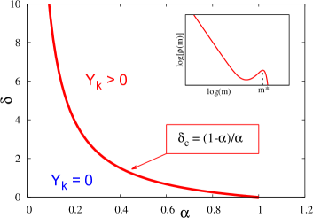
Figure 2: Main: Phase diagram for the values of the participation ratio in the ($\alpha$, $\delta$) plane in the presence of a super-extensive constraint on the total value of the mass $\sum_{i=1}^{N}m_{i}=\tilde{\rho}N^{1+\delta}$. The (red) continuous line marks the separation of the condensed phase ($\lim_{N\to\infty}Y_{k}>0$) and the homogeneous phase ($\lim_{N\to\infty}Y_{k}=0$). Inset: schematic representation of the marginal probability distribution of the local mass, $p(m)$, in the presence of condensation, namely in the whole region $\delta\geq\delta_{c}$.

Below, we evaluate the distribution $p(m)$ and the participation ratio $Y_{k}$ for $\alpha<1$ in the three cases $\delta<\delta_{c}$, $\delta>\delta_{c}$ and $\delta=\delta_{c}$ respectively.

IV.2 Case $\delta<\delta_{c}$: Homogeneous phase

As we have seen above, the system remains homogeneous for $\alpha<1$ and $\delta<\delta_{c}$, and the equivalence between canonical and grand-canonical ensembles holds. One can thus more conveniently perform calculations in the grand-canonical ensemble, with a chemical potential $\mu_{N}$ which depends on $N$, and which will be determined below as a function of the total mass. The single-mass distribution $p(m)$ simply reads

$$p(m)\approx f(m)\,e^{-\mu_{N}m}\qquad(0<m<M),$$ (33)

where we have neglected the correction to the normalization factor, as the latter remains very close to $1$ since $\mu_{N}$ is very small. Note that the distribution $p(m)$ monotonously decays at large $m$ as

$$p(m)\approx\frac{A}{m^{1+\alpha}}\,e^{-\mu_{N}m}$$ (34)

as is typical for a homogeneous phase. The $k$-th moment of this distribution is obtained for $k>\alpha$ as

$$\langle m^{k}\rangle = \int_{0}^{M}dm\,m^{k}p(m)$$

$$\approx A\int_{0}^{\infty}dm\,m^{k-1-\alpha}e^{-\mu_{N}m}=\frac{A\,\Gamma(k-\alpha)}{\mu_{N}^{k-\alpha}}.$$

The value of $\mu_{N}$ is then determined from the condition $\langle m\rangle=M/N=\tilde{\rho}N^{\delta}$, yielding

$$\mu_{N}=\left[\frac{A}{\tilde{\rho}}\,\Gamma(1-\alpha)\right]^{1/(1-\alpha)}\,N^{-\delta/(1-\alpha)}.$$ (36)

The participation ratio $Y_{k}$ is then given by

$$Y_{k}=K\tilde{\rho}^{(k-1)/\delta_{c}}\,N^{-(k-1)(\delta_{c}-\delta)/\delta_{c}}$$ (37)

with

$$K=A^{1-\omega}\,\frac{\Gamma(k-\alpha)}{\Gamma(1-\alpha)^{\omega}},\qquad\omega=\frac{k-\alpha}{1-\alpha},$$ (38)

and where $\delta_{c}$ is defined in Eq. (32). One thus obtains that $Y_{1}=1$ as it should, and that for $k>1$, $Y_{k}\to 0$ when $N\to\infty$, which confirms the absence of condensation for $\delta<\delta_{c}$. Yet, it is interesting to note that the decay of $Y_{k}$ becomes slower when increasing $\delta$, and becomes approximately logarithmic in $N$ when $(\delta_{c}-\delta)/\delta_{c}\ll 1$.

IV.3 Case $\delta>\delta_{c}$: Condensed phase

When $\delta>\delta_{c}$ (and $\alpha<1$), the partition function $Z_{N,\delta}(\tilde{\rho})$ can no longer be evaluated by a saddle-point method, and equivalence of ensembles breaks down, so that one has to work in the canonical ensemble. From Eq. (28), the Laplace transform $\hat{\mathcal{Z}}_{N,\delta}(s)$ reads in the large $N$ limit, using the small-$s$ behavior $g_{\alpha}(s)\approx 1-as^{\alpha}$,

$$\hat{\mathcal{Z}}_{N,\delta}(s)=N^{-1-\delta}\,\left(1-\frac{as^{\alpha}}{N^{\nu}}\right)$$ (39)

with $\nu=\alpha(1+\delta)-1$ (note that Eq. (39) is not restricted to small $s$ values).

By assuming a scaling function $G(x)$ which satisfies the normalization condition $\int_{0}^{\infty}G(x)\,dx=1$ and which has the asymptotic behaviour $G(x)\approx A/x^{1+\alpha}$ for $x\to\infty$, one can try to write the partition function $Z_{N,\delta}(\tilde{\rho})$ in direct space as

$$Z_{N,\delta}(\tilde{\rho})\approx N^{-1-\delta+\nu/\alpha}G(\tilde{\rho}N^{\nu/\alpha}).$$ (40)

It is then not difficult to check that the expression in Eq. (40) is (asymptotically in $N$) the correct one: the expansion for small $s$ of its Laplace transform corresponds precisely to the expression of $\hat{\mathcal{Z}}_{N,\delta}(s)$ in Eq. (39).

From the knowledge of $Z_{N,\delta}(\tilde{\rho})$ one can then compute the distribution $p(m)$, which reads as

$$p(m) = \frac{f(m)}{Z_{N,\delta}(\tilde{\rho})}\,Z_{N-1,\delta}\left(\tilde{\rho}-\frac{m}{(N-1)^{1+\delta}}\right)$$ (41)

$$\approx \frac{f(m)}{G(\tilde{\rho}N^{\delta-\delta_{c}})}\,G\left(\tilde{\rho}N^{\delta-\delta_{c}}-\frac{m}{N^{1/\alpha}}\right)$$

and has a non-monotonous shape, as seen by evaluating $p(m)$ in the regime $m\sim xM$ with $0<x<1$, which leads to

$$p(xM)\approx\frac{A}{N^{(1+\delta)(1+\alpha)}\tilde{\rho}^{1+\alpha}[x(1-x)]^{1+\alpha}}.$$ (42)

Note that the divergences at $x=0$ and $x=1$ are regularized for values of $x$ such that $x\sim M^{-1}$ and $1-x\sim M^{-1}$ respectively. The non-monotonic shape of $p(xM)$, which is schematically represented in the inset of Fig. 2, is a strong similarity that the constrained condensation for $\alpha<1$ (and superextensive total mass) bears with the constrained condensation for $\alpha>1$ (and extensive total mass). At the same time such a non-monotonic shape of $p(m)$ is a remarkable qualitative difference with the case of unconstrained condensation found for the same range of the exponent, $\alpha<1$, in which case the local mass distribution decays monotonously at large values as $p(m)\sim 1/m^{1+\alpha}$. Interestingly, the expression (41) of $p(m)$ can be rewritten as

$$p(m)\approx\frac{f(m)}{G(\tilde{\rho}N^{\delta-\delta_{c}})}\,G\left(\frac{M-m}{N^{1/\alpha}}\right)$$ (43)

with $M=\tilde{\rho}N^{1+\delta}$, which shows that the ‘bump’ occuring for $m\approx M$ has a width $\sim N^{1/\alpha}$. Hence its relative width scales as $N^{1+\delta}/N^{1/\alpha}=1/N^{\delta-\delta_{c}}$ and thus goes to zero when $N\to\infty$ for $\delta>\delta_{c}$. It would thus be legitimate in this case to call the bump a condensate, because it has a well-defined mass $M_{\rm cond}\sim M$.

To complete the analysis, let us compute the participation ratio $Y_{k}$. In the large $N$ limit, the moment $\langle m^{k}\rangle=\int_{0}^{M}dm\,m^{k}p(m)$ can be computed as, using the change of variable $v=\tilde{\rho}N^{\delta-\delta_{c}}-m/N^{1/\alpha}$,

$$\langle m^{k}\rangle\approx\frac{M^{k}}{N}\int_{0}^{M/N^{1/\alpha}}dv\,\left(1-\frac{vN^{1/\alpha}}{M}\right)^{k-1-\alpha}G(v)$$ (44)

where we have used the asymptotic (large argument) behavior of $f(m)\sim A/m^{1+\alpha}$ and $G(x)\sim A/x^{1+\alpha}$. It is then easy to show (see Appendix A) that the integral in Eq. (44) tends to $\int_{0}^{\infty}dv\,G(v)=1$ when $N\rightarrow\infty$. One thus simply gets

$$\langle m^{k}\rangle\approx\frac{M^{k}}{N}$$ (45)

which, using $Y_{k}=N\langle m^{k}\rangle/M^{k}$, immediately leads to the conclusion that $Y_{k}=1$ in the limit $N\to\infty$. Hence, as anticipated above, a strong condensation occurs for $\delta>\delta_{c}$ and $\alpha<1$, in the sense that the condensate carries almost all the mass present in the system.

IV.4 Case $\delta=\delta_{c}$: Marginal condensed phase

For $\alpha<1$ and $\delta=\delta_{c}$, the Laplace transform of the partition function reads for large $N$

$$\hat{\mathcal{Z}}_{N,\delta_{c}}(s)=N^{-1/\alpha}\,e^{-as^{\alpha}}$$ (46)

from which the partition function is obtained as

$$\mathcal{Z}_{N,\delta_{c}}(\tilde{\rho})=N^{-1/\alpha}\,H(\tilde{\rho})$$ (47)

where the function $H(\tilde{\rho})$ is independent of $N$ and is defined by its Laplace transform,

$$\int_{0}^{\infty}d\tilde{\rho}\,e^{-s\tilde{\rho}}H(\tilde{\rho})=e^{-as^{\alpha}}$$ (48)

($H$ is actually a one-sided Lévy distribution). The small $s$ behavior $e^{-as^{\alpha}}\approx 1-as^{\alpha}$ implies the large $\tilde{\rho}$ behavior

$$H(\tilde{\rho})\approx\frac{A}{\tilde{\rho}^{1+\alpha}}$$ (49)

where again $A$ is defined from the large $m$ behavior $f(m)\approx A/m^{1+\alpha}$.

The distribution $p(m)$ is given for large $N$ by

$$p(m)=\frac{f(m)}{H(\tilde{\rho})}\,H\left(\frac{M-m}{N^{1/\alpha}}\right).$$ (50)

with $M=\tilde{\rho}N^{1/\alpha}$. It is interesting to evaluate $p(m)$ in the regime where $m\sim xM$ with $0<x<1$, which leads to

$$p(xM)\approx\frac{A}{N^{1+1/\alpha}\tilde{\rho}^{1+\alpha}H(\tilde{\rho})}\,\frac{H\Big{(}\tilde{\rho}(1-x)\Big{)}}{x^{1+\alpha}}.$$ (51)

For large enough $\tilde{\rho}$, the shape of $p(m)$ is not monotonous, since the large $\tilde{\rho}$ expansion of Eq. (51) yields

$$p(xM)\approx\frac{A}{N^{1+1/\alpha}\tilde{\rho}^{1+\alpha}[x(1-x)]^{1+\alpha}}$$ (52)

with a regularization of the divergence appearing at $x=1$ for $1-x\sim\tilde{\rho}^{-1}$, and of the divergence at $x=0$ for $x\sim M^{-1}$. So here again, a bump appears in the distribution, but its width scales as $N^{1/\alpha}$ as seen from Eq. (50), so that the relative width remains of the order of one. Following EMZ06 , one may call this bump a ‘pseudo-condensate’.

The above argument on the existence of the bump in the distribution $p(m)$ was based on a large $\tilde{\rho}$ limit. The explicit example studied in EMZ06 indeed shows that the bump may disappear below a certain value of $\tilde{\rho}$.

We now turn to the evaluation of the moment $\langle m^{k}\rangle$. Using the change of variable $v=\tilde{\rho}-m/N^{1/\alpha}$, as well as the asymptotic (large argument) behaviors of $f(m)$ and $H(\tilde{\rho})$, the moment $\langle m^{k}\rangle$ can be evaluated as

$$\langle m^{k}\rangle=\tilde{\rho}^{1+\alpha}N^{-1+k/\alpha}\int_{0}^{\tilde{\rho}}dv\,(\tilde{\rho}-v)^{k-1-\alpha}H(v).$$ (53)

It follows that $Y_{k}=N\langle m^{k}\rangle/M^{k}$ is given by

$$Y_{k}=\frac{1}{\tilde{\rho}^{k-1-\alpha}}\int_{0}^{\tilde{\rho}}dv\,\left(\tilde{\rho}-v\right)^{k-1-\alpha}H(v)$$ (54)

which is one of the main results of this paper. Note that the convergence of the integral at the upper bound implies $k-\alpha>0$. Note also that the integral in Eq. (54) is a convolution, which in some cases may be conveniently evaluated using a Laplace transform, given that $H(\tilde{\rho})$ is known through its Laplace transform. For a numerical evaluation of $Y_{k}$, one may thus compute analytically the Laplace transform of the integral in Eq. (54), yielding

$$\mathcal{L}\Big{(}\tilde{\rho}^{k-1-\alpha}Y_{k}(\tilde{\rho})\Big{)}=\frac{\Gamma(k-\alpha)}{s^{k-\alpha}}\,e^{-as^{\alpha}}$$ (55)

and perform numerically the inverse Laplace transform.

The Laplace transform approach is also convenient to determine analytically the small $\tilde{\rho}$ behavior of $Y_{k}$, since the inverse Laplace transform can be evaluated through a saddle-point calculation in this limit. One finds

$$Y_{k}\approx B\,\tilde{\rho}^{\lambda}\,e^{-c/\tilde{\rho}^{\alpha/(1-\alpha)}}$$ (56)

with parameters $\lambda$, $c$ and $B$ given by

$$\lambda = \frac{\alpha(2k-2\alpha-1)}{2(1-\alpha)}$$ (57)

$$c = \frac{1-\alpha}{\alpha}\,(\alpha a)^{1/(1-\alpha)}$$ (58)

$$B = \frac{\Gamma(k-\alpha)}{\sqrt{2\pi(1-\alpha)}}\,(\alpha a)^{\frac{1+2\alpha-2k}{2-2\alpha}}$$ (59)

More detailed calculations on the derivation of Eq. (56) are reported in Appendix A.

In the large $\tilde{\rho}$ limit, it is easy to show that $Y_{k}$ goes to $1$, following a procedure similar to the one used in the case $\delta>\delta_{c}$. It is of interest to compute the first correction in $\tilde{\rho}$ (see Appendix A), and one finds

$$Y_{k}\approx 1-\frac{B^{\prime}}{\tilde{\rho}^{\alpha}}$$ (60)

with

$$B^{\prime}=\frac{A}{\alpha}\,\frac{\Gamma(1-\alpha)\,\Gamma(k-\alpha)}{\Gamma(k-2\alpha)}.$$ (61)

Note in particular that if $\alpha\ll 1$, the convergence of $Y_{k}$ to $1$ is very slow.

In summary, one has in the case $\delta=\delta_{c}$ a non-standard, weak condensation effect, which does not correspond to the genuine condensation effect reported in the literature BBJ97 ; MKB98 ; GSS03 ; MEZ05 ; EMZ06 ; EH05 ; S08-leshouches ; HMS09 ; WCBE14 ; EW14 . Here, the weak condensation effect simply means that the participation ratio takes a nonzero value in the infinite size limit, indicating that a few random variables carry a finite fraction of the sum. However, as mentioned above, there is no well-defined condensate that would coexist with a fluid phase. Depending on the generalized density $\tilde{\rho}$, the marginal distribution $p(m)$ either decreases monotonously, or has a bump which corresponds only to a pseudo-condensate, since the relative width of the bump remains of the order of one, see Eq. (50). In addition, the line $\delta=\delta_{c}$ does not correspond to a well-defined transition line in the $(\alpha,\delta)$ plane, in the sense that the state of the system continuously depends on the generalized density $\tilde{\rho}$, as shown by the expression of the participation ratio $Y_{k}$ given in Eq. (54).

V Conclusion

The general motivation of this work was to better understand the connection between condensation in the unconstrained case and in the constrained case with extensive mass, because condensation occurs on opposite ranges of the exponent $\alpha$ (which defines the power-law decay of the unconstrained probability distribution), respectively $\alpha<1$ and $\alpha>1$. To this aim, we have studied condensation in the case where the total mass is constrained to a superextensive value $M=\tilde{\rho}N^{1+\delta}$, where $\delta>0$, motivated by the fact that the typical scaling of the total mass is also superextensive, $M\sim N^{1/\alpha}$, when condensation takes place in the unconstrained case, which happens for $\alpha<1$.

We indeed found that the case of a fixed superextensive total mass interpolates in a sense between the case with a fixed extensive mass and the unconstrained case: condensation is found for values of the power law exponent in the interval $0<\alpha<1$, as in the case of unconstrained condensation, but with qualitative features more similar to the case of constrained condensation with extensive mass: for $\delta>\delta_{c}$ (and for $\delta=\delta_{c}$ at large enough $\tilde{\rho}$) the marginal distribution $p(m)$ of the local mass has a secondary peak related to the condensate fraction, at variance with unconstrained case where $p(m)$ decays monotonously for increasing values of $m$.

The inclusion in the problem of the new parameter $\delta$, which characterizes the superextensive scaling $M\sim N^{1+\delta}$ of the total mass, allowed us to draw the two-dimensional ($\alpha$, $\delta$) phase diagram shown in Fig. 2. At variance with the two models usually studied in the literature, where condensation takes place either for $\alpha<1$, without the constraint, or for $\alpha>1$, with constrained extensive mass, in the case of a constrained superextensive mass condensation is found both for $\alpha<1$ ( when $\delta>\delta_{c}$) and for $\alpha>1$ ( when $\delta>0$).

More in detail, we have shown that as soon as $\delta>0$, constrained condensation occurs for any $\alpha>1$, irrespective of the value of the generalized density $\tilde{\rho}$, when the system is constrained to have a superextensive value of the mass. This case is qualitatively similar to the case of an extensive mass $M=\rho N$ with a large density $\rho$. For $\alpha<1$, a weak form of condensation occurs if $\delta\geq\delta_{c}(\alpha)$, in the sense that the participation ratio takes a nonzero value in the infinite $N$ limit. Here, $1+\delta_{c}=1/\alpha$ is precisely the scaling exponent of the mass in the unconstrained case. When $\delta>\delta_{c}$, condensation takes the form of a bump with vanishing relative width in the marginal distribution $p(m)$. It thus shares similarities with the standard condensation phenomenon. When $\delta=\delta_{c}$, only a pseudo-condensate with non-vanishing relative fluctuations appears, or the distribution $p(m)$ may even decay monotonously. This confirmed by the expression Eq. (54) of $Y_{k}$ ($\alpha<1$ and constraint to superextensive mass with $\delta=\delta_{c}$), which differs from Eq. (25) obtained in the case of $\alpha>1$ and a fixed extensive mass. The situation is thus different from standard condensation, but the nonzero asymptotic value of the participation ratio indicates that some non-trivial phenomenon (that we call weak condensation) takes place.

To conclude, we note that the qualitative idea that condensation occurs when one imposes a total mass larger than the ‘natural’ mass the system would have in the unconstrained case remains valid: this is always the case for $\alpha>1$ (both for extensive and superextensive constraints), but it is also the case to some extent for $\alpha<1$, where condensation is present for $\delta>\delta_{c}$. Yet, one has to be aware that the notion of ‘natural mass’ is not firmly grounded in this case, and is just a heuristic concept associated to a typical scaling $M\sim N^{1/\alpha}$ with the system size $N$. One further subtlety is whether condensation occurs or not on the transition line. For the constrained case with an extensive mass, condensation does not occur at the critical density $\rho=\rho_{c}$. In constrast, a weak form of condensation occurs at $\delta=\delta_{c}$ (see Sec. IV.4), which may suggest a discontinuous condensation transition as a function of $\delta$. But for $\delta=\delta_{c}$ the condensation properties actually depend on the generalized density $\tilde{\rho}$, see Eq. (54), so that this weak condensation is actually continuous (in the sense that $Y_{k}$ goes to zero when $\tilde{\rho}\to 0$) if one looks on a finer scale in terms of $\tilde{\rho}$.

Appendix A Participation ratio for $M=\tilde{\rho}N^{1+\delta}$

In this appendix, we provide some technical details on the evaluation of participation ratios for $\alpha>1$, in the cases $\delta>\delta_{c}$ and $\delta=\delta_{c}$.

A.1 Case $\delta>\delta_{c}$

Considering the case $\alpha<1$ and $\delta>\delta_{c}$, we wish here to justify the approximation made to go from Eq. (44) to Eq. (45) in the evaluation of $\langle m^{k}\rangle$. Considering the integral appearing in Eq. (44) as well as its approximation, one can write, setting $V_{0}=M/N^{1/\alpha}$

$$\int_{0}^{V_{0}}dv\,G(v)-\int_{0}^{V_{0}}dv\,G(v)\left(1-\frac{v}{V_{0}}\right)^{k-1-\alpha}$$

$$\qquad\qquad=V_{0}\int_{0}^{1}du\,G(V_{0}u)\,[1-(1-u)^{k-1-\alpha}]$$

$$\qquad\qquad\approx\frac{A}{V_{0}^{\alpha}}\int_{0}^{1}\frac{du}{u^{1+\alpha}}\,[1-(1-u)^{k-1-\alpha}]$$

where we have used the change of variable $v=V_{0}u$ as well as the asymptotic behavior of the function $G(v)$. Assuming $k-\alpha>0$, the last integral in Eq. (A.1) converges, so that the difference of the two integrals in the lhs of Eq. (A.1) indeed converges to $0$ when $N\to\infty$, since $V_{0}\to\infty$ in this limit.

A.2 Case $\delta=\delta_{c}$

We discuss here the asymptotic, small $\tilde{\rho}$ and large $\tilde{\rho}$, behavior of the participation ratio $Y_{k}$ in the case $\delta=\delta_{c}$.

Let us start by the small $\tilde{\rho}$ regime. As discussed in the main text, $Y_{k}$ can be obtained by an inverse Laplace transform, see Eq. (55). Introducing $\psi(\tilde{\rho})=\tilde{\rho}^{k-1-\alpha}Y_{k}(\tilde{\rho})$, the Laplace transform $\hat{\psi}(s)$ is given by

$$\hat{\psi}(s)=\frac{\Gamma(k-\alpha)}{s^{k-\alpha}}\,e^{-as^{\alpha}}$$ (63)

Taking the inverse Laplace transform, one has

$$\psi(\tilde{\rho})=\frac{1}{2\pi i}\int_{s_{0}-i\infty}^{s_{0}+i\infty}ds\,\frac{\Gamma(k-\alpha)}{s^{k-\alpha}}\,e^{-as^{\alpha}+s\tilde{\rho}}.$$ (64)

In order to see whether this integral can be performed through a saddle-point evaluation, we note that balancing the two terms in the argument of the exponential leads to $as^{\alpha}\sim s\tilde{\rho}$, which results in $s\sim\tilde{\rho}^{-1/(1-\alpha)}$, eventually leading to $-as^{\alpha}+s\tilde{\rho}\sim\tilde{\rho}^{-\alpha/(1-\alpha)}$ (note that the algebraic prefactor in front of the exponential does not change the location of the saddle-point). The argument can then be made sharper using the change of variable $s=z/\tilde{\rho}^{1/(1-\alpha)}$, yielding

$$-as^{\alpha}+s\tilde{\rho}=\tilde{\rho}^{-\alpha/(1-\alpha)}(-az^{\alpha}+z).$$ (65)

In this form, a diverging prefactor is obtained when $\tilde{\rho}\to 0$, so that a saddle-point calculation can indeed be performed in this limit. Defining $\phi(z)=-az^{\alpha}+z$, the saddle-point $z_{0}$ is obtained for $\phi^{\prime}(z_{0})=0$, yielding $z_{0}=(\alpha a)^{1/(1-\alpha)}$. Choosing $s_{0}=z_{0}/\tilde{\rho}^{1/(1-\alpha)}$ in the integral (64), and setting $z=z_{0}+iy$, one can write in the small $\tilde{\rho}$ limit

$$\psi(\tilde{\rho}) \approx \frac{\Gamma(k-\alpha)}{2\pi s^{k-\alpha}}\int_{-\infty}^{\infty}dy\,\exp\left(\tilde{\rho}^{\frac{\alpha}{\alpha-1}}[\phi(z_{0})-\phi^{\prime\prime}(z_{0})\frac{y^{2}}{2}]\right)$$ (66)

$$\approx \frac{\Gamma(k-\alpha)}{z_{0}^{k-\alpha}\sqrt{2\pi\phi^{\prime\prime}(z_{0})}}\,\tilde{\rho}^{\lambda}\exp\left(\phi(z_{0})\,\tilde{\rho}^{-\frac{\alpha}{1-\alpha}}\right)$$

where $\lambda$ is given in Eq. (57), thus recovering Eq. (56).

We now turn to the computation in the large $\tilde{\rho}$ limit. We have seen that the inverse Laplace transform cannot be computed through a saddle-point evaluation in this limit. We thus come back to Eq. (54) and rewrite it as

$$Y_{k}=\int_{0}^{\tilde{\rho}}dv\,\left(1-\frac{v}{\tilde{\rho}}\right)^{k-1-\alpha}H(v)$$ (67)

Since the integral $\int_{0}^{\infty}dv\,H(v)$ converges, one can approximate for large $\tilde{\rho}$ the factor $(1-v/\tilde{\rho})^{k-1-\alpha}$ in Eq. (67) by $1$, assuming $k-1-\alpha>0$. Hence, again for $\tilde{\rho}\to\infty$,

$$Y_{k}\approx\int_{0}^{\tilde{\rho}}dv\,H(v)\to\int_{0}^{\infty}dv\,H(v)=1$$ (68)

The correction to $Y_{k}=1$ can be computed as follows:

$$1-Y_{k}=\int_{\tilde{\rho}}^{\infty}dv\,H(v)+\int_{0}^{\tilde{\rho}}dv\,H(v)\left[1-\left(1-\frac{v}{\tilde{\rho}}\right)^{k-1-\alpha}\right]$$ (69)

The first integral in Eq. (69) is easily evaluated for large $\tilde{\rho}$ as

$$\int_{0}^{\tilde{\rho}}dv\,H(v)\approx\frac{A}{\alpha\tilde{\rho}^{\alpha}}.$$ (70)

The second integral in Eq. (69) can be rewritten with the change of variable $v=\tilde{\rho}u$ as

$$\tilde{\rho}\int_{0}^{1}du\,H(\tilde{\rho}u)\,[1-(1-u)^{k-1-\alpha}]$$ (71)

$$\qquad\qquad\qquad\approx\frac{A}{\tilde{\rho}^{\alpha}}\int_{0}^{1}\frac{du}{u^{1+\alpha}}[1-(1-u)^{k-1-\alpha}]\equiv\frac{A\,I}{\tilde{\rho}^{\alpha}}$$

where we have denoted as $I$ the last integral, and where we have used the asymptotic behavior of $H(\rho)$ given in Eq. (49). Assuming $k-1-\alpha>0$ (which is consistent since $k$ is in most cases of interest an integer $>1$), the integral $I$ can be computed through an integration by part, leading to

$$I=-\frac{1}{\alpha}+\frac{k-1-\alpha}{\alpha}\,\frac{\Gamma(1-\alpha)\Gamma(k-1-\alpha)}{\Gamma(k-2\alpha)}$$ (72)

where we have also used the standard result

$$\int_{0}^{1}du\,u^{\mu-1}(1-u)^{\nu-1}=\frac{\Gamma(\mu)\Gamma(\nu)}{\Gamma(\mu+\nu)}$$ (73)

for $\mu,\,\nu>0$. Then combining Eqs. (69), (70), (71) and (72), one eventually obtains Eq. (60).

References

- (1) J. Szavits-Nossan, M. R. Evans, S. N. Majumdar, Conditioned random walks and interaction-driven condensation, J. Phys. A: Math. Theor. 50, 024005 (2017).
- (2) M. Mézard, G. Parisi and M. A. Virasoro, Spin glass theory and beyond (Singapore, World Scientific 1987).
- (3) J.-P. Bouchaud and M. Mézard, Universality classes for extreme-value statistics, J. Phys A: Math. Gen. 30, 7997 (1997).
- (4) P. Bialas, Z. Burda, D. Johnston, Condensation in the Backgammon model, Nucl. Phys. B 493, 505 (1997).
- (5) S. N. Majumdar, S. Krishnamurthy, M. Barma, Nonequilibrium Phase Transitions in Models of Aggregation, Adsorption, and Dissociation, Phys. Rev. Lett. 81, 3691 (1998).
- (6) S. Grosskinsky, G. M. Schütz, H. Spohn, Condensation in the zero range process: stationary and dynamical properties, J. Stat. Phys. 113, 389 (2003).
- (7) S. N. Majumdar, M. R. Evans, R. K. P. Zia, Nature of the Condensate in Mass Transport Models, Phys. Rev. Lett. 94, 180601 (2005).
- (8) M. R. Evans, S. N. Majumdar, R. K. P. Zia, Canonical Analysis of Condensation in Factorised Steady States, J. Stat. Phys. 123, 357 (2006).
- (9) M. R. Evans, T. Hanney, Nonequilibrium statistical mechanics of the Zero-Range Process and related models, J. Phys. A: Math. Gen. 38, R195 (2005).
- (10) S. N. Majumdar, Real-space Condensation in Stochastic Mass Transport Models, Les Houches lecture notes for the summer school on “Exact Methods in Low-dimensional Statistical Physics and Quantum Computing” (Les Houches, July 2008), ed. by J. Jacobsen, S. Ouvry, V. Pasquier, D. Serban and L. F. Cugliandolo, Oxford University Press.
- (11) O. Hirschberg, D. Mukamel, G. M. Schütz, Condensation in Temporally Correlated Zero-Range Dynamics, Phys. Rev. Lett. 103, 090602 (2009).
- (12) J. Whitehouse, A. Costa, R. A. Blythe, M. R. Evans, Maintenance of order in a moving strong condensate, J. Stat. Mech. P11029 (2014).
- (13) M. R. Evans, B. Waclaw, Condensation in stochastic mass transport models: beyond the zero-range process, J. Phys. A: Math. Theor. 47, 095001 (2014).
- (14) M. R. Evans and S. N. Majumdar, Condensation and extreme value statistics, J. Stat. Mech. P05004 (2008).
- (15) J. Szavits-Nossan, M. R. Evans, S. N. Majumdar, Constraint-Driven Condensation in Large Fluctuations of Linear Statistics, Phys. Rev. Lett. 112, 020602 (2014).
- (16) J. Szavits-Nossan, M. R. Evans, S. N. Majumdar, Condensation Transition in Joint Large Deviations of Linear Statistics J. Phys. A: Math. Theor. 47, 455004 (2014).
- (17) M. Zannetti, F. Corberi, G. Gonnella, Condensation of Fluctuations in and out of Equilibrium, Phys. Rev. E 90, 012143 (2014).
- (18) F. Corberi, G. Gonnella, A. Piscitelli, Singular behavior of fluctuations in a relaxation process, J. Non-Cryst. Solids 407, 51 (2015).
- (19) M. Zannetti, The Grand Canonical catastrophe as an istance of condensation of fluctuations, Europhys. Lett. 111, 20004 (2015).
- (20) A. Crisanti, A. Sarracino, F. Zannetti, Heat fluctuations of Brownian oscillators in nonstationary processes: fluctuation theorem and condensation transition, Phys. Rev. E 95, 052138 (2017).
- (21) M. R. Evans, T. Hanney, S. N. Majumdar, Interaction driven real-space condensation, Phys. Rev. Lett. 97, 010602 (2006).
- (22) B. Mandelbrot, J. Wallis, Noah, Joseph, and operational hydrology, Water Resour. Res. 4, 909 (1968).
- (23) M. Magdziarz, Fractional Ornstein-Uhlenbeck processes. Joseph effect in models with infinite variance, Physica A 387, 123 (2008).
- (24) E. Bertin and J.-P. Bouchaud, Subdiffusion and localization in the one dimensional trap model, Phys. Rev. E 67, 026128 (2003).
- (25) B. Derrida, From random walks to spin glasses, Physica D 107, 186 (1997).
- (26) T. Mikosch, A. V. Nagaev, Large deviations of heavy-tailed sums with applications in insurance, Extremes 1, 81 (1998).