Testing and selecting cosmological models with ultra-compact radio quasars

Abstract

In this paper, we place constraints on four alternative cosmological models under the assumption of the spatial flatness of the Universe: CPL, EDE, GCG and MPC. A new compilation of 120 compact radio quasars observed by very-long-baseline interferometry, which represents a type of new cosmological standard rulers, are used to test these cosmological models. Our results show that the fits on CPL obtained from the quasar sample are well consistent with those obtained from BAO. For other cosmological models considered, quasars provide constraints in agreement with those derived with other standard probes at $1\sigma$ confidence level. Moreover, the results obtained from other statistical methods including Figure of Merit, $Om(z)$ and statefinder diagnostics indicate that: (1) Radio quasar standard ruler could provide better statistical constraints than BAO for all cosmological models considered, which suggests its potential to act as a powerful complementary probe to BAO and galaxy clusters. (2) Turning to $Om(z)$ diagnostics, CPL, GCG and EDE models can not be distinguished from each other at the present epoch. (3) In the framework of statefinder diagnostics, MPC and EDE will deviate from $\rm{\Lambda}$CDM model in the near future, while GCG model cannot be distinguished from $\rm{\Lambda}$CDM model unless much higher precision observations are available.

1 Introduction

It is strongly indicated that the Universe has entered a stage of accelerated expansion, which was confirmed by a lot of recent observations including Supernova Ia (SN Ia) (riess1998observational, ; riess2007new, ; suzuki2012hubble, ), baryon acoustic oscillation (BAO) (percival2010baryon, ), and precise measurements of the spectrum of cosmic microwave background (CMB) (spergel2003first, ; komatsu2011seven, ; hinshaw2013nine, ; ade2016planck, ). However, it remains a big puzzle in modern cosmology about the origin to the current cosmic acceleration, which gives birth to a large class of cosmological models mathematically explaining this phenomenon. In general, these cosmological scenarios are mainly split into two large categories, the first of which adheres to General Relativity and drives the current accelerated expansion through a dark energy component, while the second focus on gravitational modifications without the inclusion of exotic dark energy.

In the first scenario, the most simple candidate for dark energy is the cosmological constant $\rm{{\rm{\Lambda}}}$, in which the equation of state (EoS) of dark energy is equal to $-1$. This model, the so-called $\rm{\Lambda}$CDM, provides excellent agreements with a wide range of astronomical data so far (cao2011testing, ; li2016comparison, ). However, it is confronted with some theoretical problems including the well-known fine tuning problem and coincidence problem (weinberg1989cosmological, ). Other models allowing any constant dark energy equation of state (quintessence (ratra1988cosmological, ; peebles1988cosmology, ), phantom models (caldwell2002phantom, ), etc.), as well as models in which the dark energy equation of state is allowed to evolve with time (the well-known CPL parametrization (chevallier2001accelerating, ; linder2003cosmic, )) have been extensively studied with various astrophysical probes in the literature (cao2014cosmic, ). Meanwhile, considering the possible interaction between dark energy and dark matter, the so-called interacting dark energy model (caldera2009dynamics, ; valiviita2010observational, ; zheng2017ultra, ) could also contribute to the alleviation of the coincidence problem. Originating from different aspects of new physics, many other dynamical dark energy models such as the Chaplygin gas (kamenshchik2001alternative, ; barreiro2008wmap, ) and the holographic dark energy models (huang2004holographic, ; setare2007holographic, ; sheykhi2011interacting, ) have been explored by cosmologists for a long time. In the second scenario, significant interest in modifications to general relativity has also gained a lot attention (freese2002cardassian, ; Qi2017, ; Xu2017, ), with the aim of explaining the acceleration of the Universe without introducing dark energy.

In the face of so many competing cosmological models, many authors turned to various observational probes such as Supernovae Ia acting as standard candles ($z\sim 1.40$), strong gravitational lensing systems (cao2012constraints, ; cao2015cosmology, ), BAO, and CMB ($z\sim 1000$) acting as standard rulers, with the aim to determine which one is most favored by the observational data (cao2014cosmic, ; li2016comparison, ). However, in order to achieve this difficult goal of model filtration, it is still necessary to acquire high precision data set and develop new complementary techniques bridging the redshift gap of current data. In the past decades, different types of radio sources have been proposed as possible candidates for standard rulers in cosmological studies (buchalter1998constraining, ; gurvits1998angular, ; daly2003model, ). For instance, the size of the line emitting regions was employed as a standard ruler to study the local expansion history of the Universe, using which Ref. (watson2011new, ) actually derived the distance to Active Galactic Nuclei (AGN). Another new type of useful cosmological ruler is Super-Eddington accreting quasar, the properties of which have been extensively studied in Refs. wang2013super ; marziani2014highly . Recent studies have used the nonlinear relation between the ultraviolet and X-ray luminosity of quasars to place constraints on cosmological parameters (risaliti2015hubble, ). In this paper, we highlight the usefulness of ultra-compact structure in radio quasars as a reliable cosmic standard probe to assess some popular cosmological models. In the more recent work (cao2017a, ), a sub-sample of 120 intermediate-luminosity quasars in the redshift range of $0.46<z<2.8$ was extracted from 613 milliarcsecond ultra-compact radio sources observed by the very-long-baseline interferometry (VLBI) all-sky survey. A pioneer work using this data was also performed in Ref. (cao2017ultra, ) to probe a flat $\rm{\Lambda}$CDM model and XCDM model, in which the linear size of this standard ruler was calibrated as $l_{m}=11.03$ pc through a cosmological- model-independent method. As complementary to other cosmological standard rods, such as BAO and galaxy clusters (bonamente2006determination, ), quasars are promising objects for studying the expansion rate of the Universe at much higher redshift, thus have become an effective probe in cosmology and astrophysics (cao2017ultra, ; zheng2017ultra, ). As an extension of the previous work (cao2017ultra, ), the aim of this analysis is to test alternative cosmological models using the quasar sample and investigate its possibility to provide additional information of model discrimination compared with that provided by other standard ruler data (BAO and galaxy clusters). Two model diagnostics, the $Om$ diagnostic (sahni2008two, ) and the statefinder diagnostic (sahni2003statefinder, ), are also applied to our work.

This paper is organized as follows: In Section 2, we briefly introduce the observational data sets used. The details of the cosmological models to be considered are presented in Section 3. In Section 4, we describe the methods used to obtain the constraints for each data set. In Section 5, we perform a Markov Chain Monte Carlo (MCMC) analysis, and furthermore apply model diagnostics in Section 6. The main results are summarized in Section 7.

Figure 1: Redshift distribution of different standard ruler data. One can see a fair coverage of redshifts in the combined sample.

2 Data

Three types of standard rulers currently available are used to place constraint on different cosmological models: the compact radio quasars (QSO) data from VLBI, the angular-diameter distance ($D_{A}$) measurements derived from galaxy clusters, and the baryonic acoustic oscillations (BAO) data from large-scale structure (LSS) observations.

${\bf{QSO}}$. In our analysis, we use the angular size measurements of 120 radio quasars covering the redshift range of $0.46<z<2.76$ (cao2017ultra, ). The linear sizes of compact structure in intermediate-luminosity radio quasars ($10^{27}$ W/Hz $<L<10^{28}$ W/Hz) display negligible dependent on luminosity and redshift (cao2017a, ). We refer the reader to (cao2017a, ) for the detailed selection methodology to obtain the final sample of radio quasars explicitly presented in (cao2017ultra, ), which could serve as standard cosmological rods with intrinsic linear size calibrated to $l_{m}=11.03\pm 0.25$ pc.

Galaxy cluster. X-ray observation of intracluster medium and radio observations of Sunyaev-Zeldovich effect allow us to estimate the angular diameter distance of galaxy clusters. In this paper, we will use the $D_{A}$ measurements of 38 galaxy clusters in the redshift range of $0.16<z<0.89$. The final statistical sample with all necessary information can be found in Refs. (bonamente2006determination, ).

BAO. The third astrophysical probe applied to the joint cosmological analysis is BAO, which measures the angular-diameter distance through the clustering of galaxies perpendicular to the line of sight. The acoustic peak in the galaxy correlation function has been detected over a redshift range of $0.1<z<0.7$ with large scale surveys. The determination of the BAO scale at lower redshift, $z=0.106$, was made in the 6dFGS survey (beutler20116df, ), while the other four measurements of acoustic scale at higher redshifts were respectively obtained by SDSS-DR7 (padmanabhan20122, ), SDSS-DR9 (anderson2012Clustering, ), and the WiggleZ galaxy survey (blake2012wigglez, ). These data extensively used in nine-year WMAP analysis were summarized in Table 1 of Ref. hinshaw2013nine .

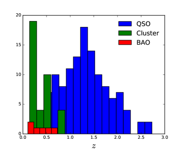
We remark here that, in order to test the cosmological models at higher redshifts, it is very necessary to turn to distance indicators located in the deeper universe. Higher-redshift radio-loud quasars are valuable additions to standard rulers used for cosmological tests, since the predictions of cosmological models can be radically different. Fig. 1 shows the redshift coverage of different standard ruler data. One can see that inclusion of quasars could result in a fair coverage of redshifts, which enables QSO an excellent complement to other observational probes at lower redshifts.

3 Cosmological models

Four cosmological models are considered with the data sets described above: Chevallier-Ploarski-Linder parametrization (CPL), Entropy Dark energy model (EDE), Generalized Chaplygin Gas Model (GCG) and modified polytropic Cardassian model (MPC). A flatness of Friedmann Robertson Walker (FRW) metric is assumed in our analysis, which is strongly supported by the recent observations (amanullah2010spectra, ; hinshaw2013nine, ). Under this assumption, the angular diameter distance can be expressed as

$${}{D_{A}(z)}\,=\,{\frac{c}{H_{0}(1+z)}}\int_{0}^{z}\,\frac{dz^{\prime}}{E(z^{\prime})}$$ (1)

where $E(z)\,=\,H(z)/H_{0}$ and $H_{0}$ is the Hubble constant, which is fixed at $67.8\pm 0.9\,\rm{km\,s^{-1}Mpc^{-1}}$ based on recent Planck results (ade2016planck, ). Moreover, in order to obtain stringent constraints on other cosmological parameters, for the CPL, EDE, and MPC models, we use the prior on the matter density parameter $\Omega_{m}$ from Planck (ade2016planck, ). It should be noted that, although the above priors always influence the cosmological analysis, conclusions should not be significantly affected concerning the core of this paper, i.e., the comparison of the confidence regions derived from different standard ruler data.

3.1 CPL model

A simple extension of the $\rm{\Lambda}$CDM model is the XCDM model with constant equation of state. However, it would be natural to consider the equation of state varying with redshifts, i.e., it could be an arbitrary function of the redshift, $w\,=\,w(z)$. One of the most popular functions is the CPL parametrization (chevallier2001accelerating, ; linder2003cosmic, )

$${w(z)}\,=\,{w_{0}+w_{a}\frac{z}{1+z}}$$ (2)

where $w_{0}$ and $w_{a}$ are the two parameters to be fitted by the observational data. Note that the $\Lambda$CDM model can be always recovered by taking $w_{0}=-1$ and $w_{a}=0$. Then the Hubble function can be expressed as

$${H(z)}\,= \,H_{0}[\Omega_{m}(1+z)^{3}+$$ (3)

$$\Omega_{DE}(1+z)^{3(1+w_{0}+w_{a})}e^{(\frac{-3w_{a}z}{1+z})}]^{1/2}$$

where $\Omega_{DE}\,=\,1-\Omega_{m}$, and the cosmological parameters in this cosmological model are ${\bf{p}}\,=\,(w_{0},w_{a})$.

3.2 EDE model

Recently, the Entropy Dark Energy model was proposed on the base of the theory of entropic gravity easson2011entropic ; easson2012entropic . In the framework of entropic gravity theory, the gravity force can be explained as a kind of entropic force related to the change of entropy, while the field of equation of gravity is obtained with the second law of thermodynamics. The EDE in the entropic gravity model arises from the surface term in the Einstein-Hilbert’s action. In the previous work of Refs. easson2011entropic ; easson2012entropic , a positive term $C_{H}H^{2}+C_{\dot{H}}{\dot{H}}$ (the overdot means a derivative with time) was added to the surface part in the action, where $C_{H}$ and $C_{\dot{H}}$ are the model parameters respectively falling into the range of $3/2\pi\leq C_{H}\leq 1$ and $0\leq C_{\dot{H}}\leq 3/2\pi$. In our work, no interaction between the DE and other cosmic components (especially matter) is assumed and one can derive the evolution of Hubble parameter as

$$H(z)\,=\,H_{0}[\eta(1+z)^{3}+(1-\eta)(1+z)^{2(C_{H}-1)/C_{\dot{H}}}]^{1/2}$$ (4)

where

$$\eta\,=\,\frac{\Omega_{m}}{1+(\frac{3}{2}C_{\dot{H}}-C_{H})}$$ (5)

It is straightforward to show that $\eta=\Omega_{m}$ when $C_{H}=3C_{\dot{H}}/2$, and the parameters to be considered in this model are ${\bf{p}}\,=\,(C_{H},C_{\dot{H}})$.

3.3 GCG model

The so-called General Chaplygin Gas model (GCG) has been widely studied to explain the accelerating universe (kamenshchik2001alternative, ; barreiro2008wmap, ; lu2009observational, ). In the GCG model, the dark sectors in the Universe, i.e., dark energy and dark matter, can be unified through an exotic equation of state. More specifically, the GCG background fluid with its energy density $\rho_{GCG}$ and pressure $p_{GCG}$ can be related with the equation of state (kamenshchik2001alternative, ) $p_{GCG}=-\frac{A}{\rho_{GCG}^{\alpha}}$, where $\rho_{GCG}\,=\,\rho_{DE}+\rho_{DM}$ is the unified energy density of dark energy and dark matter. The Universe is filled with two components, the GCG component and the baryonic matter component, i.e., $\rho=\rho_{GCG}+\rho_{b}$. Under the assumption of flat FRW metric, the Hubble parameter of this model can be expressed as

$$H(z)\,= H_{0}[\Omega_{b}(1+z)^{3}+$$ (6)

$$\Omega_{GCG}(A_{s}+(1-A_{s})(1+z)^{3(1+\alpha)})^{\frac{1}{1+\alpha}}]^{1/2}$$

where $\Omega_{GCG}=1-\Omega_{b}$ and $A_{s}=\frac{A}{\rho^{1+\alpha}}$. In our analysis, the baryonic density parameter is fixed at $\Omega_{b}=0.0484$ based on the recent Planck results ade2016planck , and the two cosmological parameters in this model are ${\bf{p}}\,=\,(A_{s},\alpha)$.

3.4 MPC model

In order to explain the cosmic acceleration from a different perspective, Freese & Lewis (2002) put forward a Cardassian model without the introduction of dark energy (freese2002cardassian, ), for which the Friedmann equation is modified as

$$H^{2}\,=\,\frac{8\pi G\rho_{m}}{3}+B\rho^{n}_{m}$$ (7)

where $\rho_{m}$ is the total matter density. We emphasize here that, in order to lead to the cosmic acceleration in this parameterization, the value of the parameter $n$ should always be $n<2/3$. Then a simple generalized case of the Cardassian model was proposed in Ref. (gondolo2002accelerating, ), in which an additional exponent $q$ was introduced. The Hubble parameter with this generalization can be written as

$$H(z)\,=\,H_{0}\{\Omega_{m}(1+z)^{3}\times[1+(\Omega_{m}^{-q}-1)(1+z)^{3q(n-1)}]^{1/q}\}^{1/2}$$ (8)

where the parameters to be constrained are ${\bf{p}}\,=\,(q,n)$. This MPC model will reduce to $\rm{\Lambda}$CDM model with $q=1$ and $n=0$.

4 Method

In the following, we consider the observational constraints on the cosmological models from observational data.

4.1 QSO

If taking milliarcsecond structure in radio quasars as individual standard rulers, the angular sizes at redshift $z$ can be written as

$$\theta(z)\,=\,\frac{l_{m}}{D_{A}(z)}$$ (9)

where $D_{A}(z)$ is the corresponding angular diameter distance mentioned above and $l_{m}$ is the intrinsic length of milliarcsecond structure in radio quasars. In this work, we take the typical value of $l_{m}=11.03\pm 0.25$ pc calibrated with cosmic chronometers, which was obtained through a new cosmology-independent calibration technique (cao2017ultra, ). Following the general classification of Active Galactic Nuclei (AGN), it is powered by the accretion of mass onto black holes in the center of galaxies and will produce jets of relativistic plasma in the central regions. There are two main physical meaning related to the linear size of this standard ruler: on the one hand, there is almost no stellar contribution when the distance from the AGN center approaches 10 pc, which is also the position at which AGN jets are typically generated (Blandford78, ); On the other hand, according to the recent analysis of the correlation between the black hole’s mass accretion and the star-formation rate, 10 pc represents the typical radius within which the two rates are almost equal to each other, a conclusion supported by the findings from both recent observations and simulations of AGN (silverman2009the, ; hopkins2009how, ). More importantly, the value of $l_{m}$ estimated from single-frequency VLBI measurements agrees very well with that obtained from multi-frequency VLBI imaging observations (pushkarev2015milky, ). Such consistency could also be seen from the comparison between the cosmological fits derived from two types of VLBI observations at different observing frequencies (Caomulti, ). The data points of the 120 QSOs are given in terms of the angular sizes, $\theta_{i}^{obs}$. One can then constrain cosmological parameters by minimizing the $\chi^{2}$ function given by

$$\chi_{QSO}^{2}\,=\,\sum_{i}^{120}{\frac{(\theta(z_{i};{\bf{p}})-\theta_{i}^{obs})^{2}}{\sigma_{i}^{2}}}$$ (10)

where $\theta(z_{i};\bf{p})$ is the theoretical value of the angular size at redshift $z$ (which is defined in Eq. (9)) and ${\bf{p}}$ represents the cosmological parameters of interest (which are specifically introduced in Section 3). $\theta_{i}^{obs}$ is the observed counterpart of the angular size for the ith quasar. Following the work of Ref. (cao2017ultra, ), in our analysis the total uncertainty expresses as $\sigma^{2}_{i}\,=\,\sigma^{2}_{sta,i}+\sigma^{2}_{sys,i}$, which includes the statistical error of observations in $\theta_{i}^{obs}$ and an additional $10\%$ systematical uncertainty accounting for the intrinsic spread in the linear size. See Table 1 of Ref. (cao2017ultra, ) for details of the quasar data and reference to the source papers.

4.2 Galaxy clusters

We can obtain the angular diameter distances by using the Sunyaev-Zeldovich effect together with x-ray emission of galaxy clusters, which can be directly used to estimate the cosmological parameters by minimizing the corresponding $\chi^{2}$ as

$$\chi_{Cluster}^{2}\,=\,\sum^{38}_{i=1}\,\frac{[D_{A}^{th}(z_{i};{\bf{p}})-D_{A}^{obs}(z_{i})]^{2}}{\sigma^{2}_{D_{A},i}}$$ (11)

Here $D_{A}^{th}(z_{i};{\bf{p}})$ is the theoretical angular diameter distance at redshift $z_{i}$, which is defined in Eq. (1). $D_{A}^{obs}(z_{i})$ is the observed angular diameter distance of the $i$th galaxy cluster with total uncertainty defined as $\sigma^{2}_{D_{A},i}=\sigma^{2}_{mod}+\sigma^{2}_{stat}+\sigma^{2}_{sys}$, where the modeling error ($\sigma_{mod}$), statistical error ($\sigma_{stat}$) and systematical error ($\sigma_{sys}$) are explicitly shown in Table 2-3 in Ref. bonamente2006determination .

4.3 BAO

Compared with the previous works involving BAO as a standard ruler (cao2010testing, ; cao2011testing, ; cao2011constraints, ), we use the measurement of distance ratio $r_{s}(z_{d})/D_{V}(z)$ or $D_{V}(z)/r_{s}$ from the BAO peak in the distribution of SDSS luminous red galaxies, which contains the main information of the observations of LSS. Here $r_{s}(z_{d})$ is the comoving sound horizon at the drag epoch, where the redshift $z_{d}$ at the baryonic drag epoch is fitted with the formula proposed in Ref. eisenstein1998baryonic . $D_{V}(z)$ is the effective distance given by

$$D_{V}(z)\,=\,\left[(1+z)^{2}D_{A}^{2}(z)\frac{cz}{H(z)}\right]^{1/3}$$ (12)

where $D_{A}$ is the angular diameter distance and $H(z)$ is Hubble parameter. The $\chi^{2}$ function for BAO is defined as

$$\chi^{2}_{BAO}=\bf(x-d)^{T}(C_{BAO}^{-1})(x-d),$$ (13)

where

$${\bf{x-d}}=[r_{s}/D_{V}(0.1)-0.336,D_{V}(0.35)/r_{s}-8.88,$$ (14)

$$D_{V}(0.57)/r_{s}-13.67,r_{s}/D_{V}(0.44)-0.0916,$$

$$r_{s}/D_{V}(0.60)-0.0726,r_{s}/D_{V}(0.73)-0.0592]$$

and $C^{-1}_{BAO}\,=$

$$\left(\begin{array}[]{cccccc}4444.4&0&0&0&0&0\\ 0&34.602&0&0&0&0\\ 0&0&20.661157&0&0&0\\ 0&0&0&24532.1&-72584.4&12099.1\\ 0&0&0&-25137.7&134598.4&-64783.9\\ 0&0&0&12099.1&-64783.9&128837.6\\ \end{array}\right)$$

is the corresponding inverse covariance matrix (hinshaw2013nine, ).

4.4 Joint analysis

We will present a combined analysis of the above three tests to fit theoretical models to observational data. Meanwhile, in order to make a good comparison with the quasar sample, a joint analysis with galaxy clusters and BAO data sets is also performed in this analysis. The $\chi^{2}$ function of the above two combined analysis are respectively expressed as

$$\chi^{2}_{total}\,=\,\chi^{2}_{BAO}+\chi^{2}_{Cluster}+\chi^{2}_{QSO}$$ (16)

and

$$\chi^{2}_{BAO+Cluster}\,=\,\chi^{2}_{BAO}+\chi^{2}_{Cluster}$$ (17)

Table 1: The marginalized 1$\sigma$ errors of the model parameters for different cosmological scenarios, as well as their corresponding $FoM$, estimated from QSO, BAO, galaxy clusters and the joint analysis.

Data Set	FoM	$w_{0}$	$w_{a}$
QSO	$27.40$	$-0.91^{+0.48}_{-0.54}$	$-0.4^{+2.9}_{-2.3}$
BAO	$1.61$	$-1.12^{+0.31}_{-0.35}$	$-1.8^{+3.2}_{-2.1}$
Cluster	$29.35$	$>-0.286$	$-5.7^{+1.3}_{-2.8}$
Cluster+BAO	$20.90$	$-0.23^{+0.22}_{-0.36}$	$-4.0^{+4.3}_{-3.4}$
All	$111.758$	$-0.72^{+0.19}_{-0.32}$	$-1.43^{+1.7}_{-0.87}$
Data Set	FoM	$C_{\dot{H}}$	$C_{H}$
QSO	$117950.7$	$>0.327$	$0.793^{+0.099}_{-0.057}$
BAO	$62181.8$	$>0.419$	$0.675^{+0.14}_{-0.096}$
Cluster	$104122.7$	$0.367^{+0.11}_{-0.046}$	$>0.875$
Cluster+BAO	$1949008.7$	$>0.470$	$0.933^{+0.057}_{-0.022}$
All	$3185494.1$	$>0.469$	$0.895^{+0.040}_{-0.027}$
Data Set	FoM	$A_{s}$	$\alpha$
QSO	$5819.5$	$0.761^{+0.080}_{-0.075}$	$>-0.0945$
BAO	$4424.4$	$0.890^{+0.036}_{-0.168}$	$0.24\pm 0.39$
Cluster	$963.7$	$0.575^{+0.108}_{-0.050}$	$<-0.0954$
Cluster+BAO	$64683.43$	$0.621^{+0.082}_{-0.067}$	$-0.25^{+0.17}_{-0.14}$
All	$146723.6$	$0.708\pm 0.040$	$-0.05^{+0.10}_{-0.16}$
Data Set	FoM	$\beta$	$n$
QSO	$1.99$	$0.56^{+5.34}_{-0.36}$	$0.46^{+0.166}_{-0.472}$
BAO	$1.89$	$0.61^{+4.49}_{-0.41}$	$0.09^{+0.33}_{-0.45}$
Cluster	$2.66$	$0.32^{+5.5}_{-0.33}$	$0.56^{+0.041}_{-0.31}$
Cluster+BAO	$1.70$	$0.38^{+3.02}_{-0.28}$	$0.122^{+0.216}_{-0.286}$
All	$3.94$	$0.59^{+3.0}_{-0.33}$	$0.46^{+0.031}_{-0.29}$

5 Results and discussion

For all cosmological models described in Section 3, we estimate the constraint ability of different angular diameter distance data, QSO, BAO, galaxy clusters, BAO+Cluster and BAO+Cluster+QSO, by minimizing the $\chi^{2}$ function given in Sect. 4. Furthermore, the Figure of Merit (FoM) (mortonson2010figures, ) is also applied to quantify the constraining power of each data (especially the quasar sample) on cosmological model parameters.

5.1 CPL

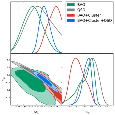
The best fits for CPL parameters ${w_{0},w_{a}}$ and the estimated $\chi^{2}$ from different data sets are shown in Table 1. The $1\sigma$, $2\sigma$ contours of the model parameters are presented in Fig.2. As can be seen from Table 1 and Fig.2, the fitting results from QSO are in good agreement with those from BAO, whereas in tension with the results from galaxy cluster data. Notice that concordance $\rm{\Lambda}$CDM cosmology ($w_{0}=-1$, $w_{a}=0$) is consistent with the quasar and BAO standard ruler data at less than 1$\sigma$ level. More importantly, compared with the previous literature using other independent and precise experiments (cao2011constraints, ; cao2012testing, ; cao2015cosmology, ), the currently compiled quasar data may improve the constraints on model parameters significantly, in the framework of CPL parametrization. When adding QSO data set to the joint data set of BAO and galaxy cluster, we will get more precise assessment of ${w_{0},w_{a}}$, which is consistent with that obtained from the recent Planck CMB data (ade2016planck, ) as well as the combination of the CMB measurements from Atacama Cosmology Telescope (ACT) and the South Pole Telescope, BAO and $H_{0}$ measurements (hinshaw2013nine, ).

Figure 2: $1\sigma$,$2\sigma$ contours of the CPL model parameters $w_{0}$ and $w_{a}$ obtained from different standard ruler data.

Figure 3: $1\sigma$,$2\sigma$ contours of the EDE model parameters $C_{\dot{H}}$ and $C_{H}$ obtained from different standard ruler data.

5.2 EDE

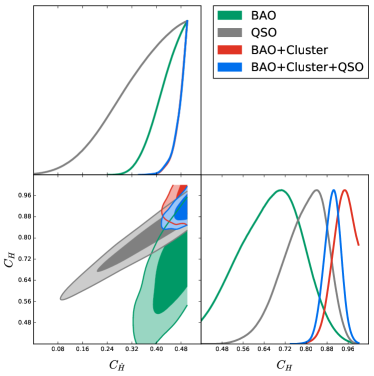
Table 1 shows the best fits of EDE parameters $(C_{\dot{H}},C_{H})$ and the $\chi^{2}$ derived from different observational data sets. Although the exact value of $C_{\dot{H}}$ are not independently obtained with QSO or BAO, appreciable consistency between the same type of probes (standard rulers) is indeed revealed in our analysis. On the other hand, it is clear that the quasar data set could provide constraints on the other parameter $C_{H}$ comparable to the other two types of standard probes. These implications can be more clearly seen from the corresponding contours for EDE model, which are explicitly presented in Fig. 3. Fitting results from the joint angular diameter distance data of QSO+BAO+Cluster give the best-fit parameters $C_{\dot{H}}>0.469$ and $C_{H}=0.895^{+0.040}_{-0.027}$, which agree very well with the results yielded from the luminosity distance data including 307 Type Ia Supernovae: $C_{\dot{H}}=0.415\pm 0.061$ and $C_{H}=0.813\pm 0.056$ (mathew2016evolution, ).

Figure 4: $1\sigma$,$2\sigma$ contours of the GCG model parameters $A_{s}$ and $\alpha$ obtained from different standard ruler data.

5.3 GCG

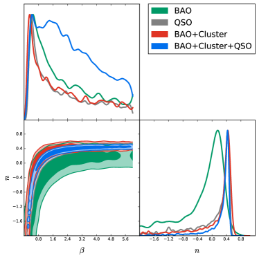
Working on the GCG model, we obtain the fitting results from different combinations of observational data, which are displayed in Table. 1 and Fig. 4. The excellent consistency between the three types of standard rulers can be clearly seen through the comparison of these plots. The joint analysis with standard rulers provides the best-fit parameters and the marginalized 1$\sigma$ constraints as $A_{s}=0.708\pm 0.040$ and $\alpha=-0.05^{+0.10}_{-0.16}$. For comparison, it is necessary to refer to the previous results obtained with other astrophysical measurements. The results obtained with the combination analysis of the X-ray mass fractions of galaxy clusters, the dimensionless coordinate distance to SN I and FRIIb radio galaxies gave $A_{s}\,=\,0.70^{+0.16}_{-0.17}$ and $\alpha\,=\,-0.09^{+0.54}_{-0.33}$ (zhu2004generalized, ). The former work done in Ref.  (wu2007generalized, ) with the joint data of 9 Hubble parameters data points, 115 SN Ia and BAO peak at $z\,=\,0.35$ showed that $0.67\leq A_{s}\leq 0.83$ and $-0.21\leq\alpha\leq 0.42$. Recent work done in lu2009observational indicated $A_{s}\,=\,0.73\pm 0.06$ and $\alpha\,=\,-0.09^{+0.15}_{-0.15}$, which strengthens the indication that joint analysis of cosmic standard rulers (QSO+BAO+Cluster) could provide consistent but more stringent fitting results compared with these previous results.

Figure 5: $1\sigma$,$2\sigma$ contours of the MPC model parameters $\beta$ and $n$ obtained from different standard ruler data.

5.4 MPC

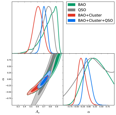
All of the fitting results obtained with QSO, BAO, Cluster and the joint data are presented in Table 1. The $1\sigma$, $2\sigma$ contours of the MPC model parameters $\beta$ and $n$ are also illustrated in Fig. 5. The results from QSO, BAO and galaxy cluster are consistent with each other within $1\sigma$ confidence level. Several authors have tested the MPC model using various data sets. For instance, Cosmic All-Sky Survey (CLASS) lensing sample (alcaniz2005constraints, ) gave $\beta\,=\,0.05$, $n\,=\,-2.32$, which is in tension with our results from QSO+BAO+Cluster. However, It is important to note that the shape of the constraint contours derived in our analysis are very similar to those shown in Refs. (alcaniz2005constraints, ; feng2010cardassian, ; liang2011latest, ; li2011testing, ; magana2015magnified, ). Moreover, the results obtained with standard rulers turned out to correspond well with previous works. Our results are similar to the results obtained with SN Ia+BAO+WMAP5 ($\beta\,=\,0.48^{+2.020}_{-0.080}$, $n\,=\,-0.600^{+0.980}_{-0.450}$) and SN Ia+BAO+CMB data sets ($\beta\,=\,1.098^{+1.015}_{-0.465}$, $n\,=\,-0.041^{+0.364}_{-0.964}$) at $1\sigma$ confidence level (feng2010cardassian, ). More recent works (magana2015magnified, ) have suggested the cutoffs of $0.45\,<\beta\,<1.05$ and $-0.8\,<n\,<0.05$, which achieved a similar precision to our work.

Figure 6: FoM for different cosmological models using QSO, BAO, galaxy cluster observations and the joint data sets.

5.5 Figure of Merit

As discussed above, the method of using the angular size measurements of compact structure in radio quasars distance could provide a complementary and effective probe in cosmological applications. However, in order to quantify the constraining power of the quasar sample, we introduce the Figure of Merit (FoM) (albrecht2006report, ; mortonson2010figures, ), a useful statistical tool originally defined by the Dark Energy Task Force as the inverse of the area enclosed by the $95\%$ confidence level contour of CPL parameters, $(w_{0},w_{a})$. Later there was a more general definition of FoM (wang2008figure, )

$$\text{FoM}\,=\,\frac{1}{\sqrt{\text{det\,Cov}(f_{1},f_{2},f_{3},...)}}$$ (18)

where $\text{Cov}(f_{1},f_{2},f_{3},...)$ is the covariance matrix of the cosmological parameters $f_{i}$. Note that a larger FoM corresponds to a smaller error ellipse, which therefore denotes a tighter constraints on the cosmological parameters.

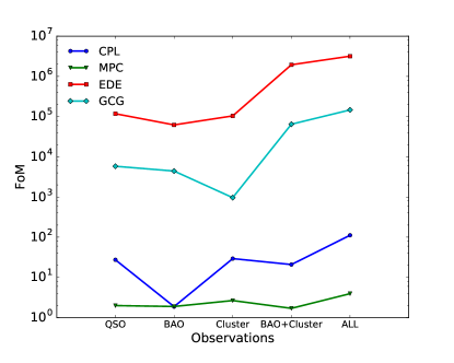
We have calculated the FoM of the cosmological models for each data set analyzed, which is explicitly summarized in Table 1. A graphical representation of the FoM results is also provided in Fig. 6, which directly shows the results in the FoM test for each cosmological model. Out of all the candidate models considered, it is obvious that the QSO data could provide better statistically constraints on cosmological parameters than BAO. This could attribute to the large sample size and the higher redshift range covered by QSOs in comparison to other cosmological probes. When taking galaxy cluster observations into consideration, quasars perform better than galaxy clusters in the framework of two cosmological models, GCG and EDE models. On the other hand, when comparing the FoM of BAO+Cluster and that of all observations, we find the inclusion of the QSO sample will generate more stringent cosmological constraints.

6 Model diagnostics

In order to discriminate the four cosmological scenarios considered in this paper, it is important to find sensitive and robust diagnostics to illustrate the dynamic behavior of different cosmologies. As is well known, the expansion rate of the Universe can be expressed by the Hubble parameter $H\,=\,\dot{a}/a$, where $a$ is the scale factor, while the rate of cosmic acceleration ia always quantified by the deceleration parameter

$$q\,=\,-\frac{\ddot{a}}{aH^{2}}\,=\,-\frac{a\ddot{a}}{{\dot{a}}^{2}}$$ (19)

However, it is very difficult for the Hubble parameter $H$ and the deceleration parameter $q$ to accurately distinguish cosmological models cause all the models considered will give similar results, e.g., $\ddot{a}\,>\,0$ and $H\,>\,0$ or $q\,<\,0$, which encourages us to invoke some newer and more effective quantities to substitute the two original parameters. In this work, we will take the $Om$ diagnostic and the statefinder diagnostic into consideration.

Figure 7: The evolution of $Om(z)$ versus the redshift $z$ for different cosmological models.

It is well known that $Om(z)$ is a combination of the Hubble parameter and the redshift, which provides a null test of dark energy being a cosmological constant at different stages for the $\rm{\Lambda}$CDM model (sahni2008two, ). Therefore, this diagnostic, which has been extensively used to discriminate different cosmological models as well as $\rm{\Lambda}$CDM model (ding2015is, ; zheng2016what, ), can be defined as

$$Om(z)\,=\,\frac{E^{2}{(z)}-1}{(1+z)^{3}-1}$$ (20)

where $E(z)\,=\,H(z)/H_{0}$. In the basic $\rm{\Lambda}$CDM model neglecting the radiation at low redshifts, one can easily get

$$E^{2}_{\rm{\Lambda}CDM}(z)=\Omega_{m}(1+z)^{3}+(1-\Omega_{m})$$ (21)

The combination of Eq. (20) and Eq. (21) will lead to

$$Om(z)\,|_{\rm{\Lambda}CDM}=\,\Omega_{m}$$ (22)

It is obvious that $Om(z)$ should be constant and exactly equal to the present mass density parameter $\Omega_{m}$ if the $\rm{\Lambda}$CDM model is the true one, while for other cosmological models, the $Om(z)$ diagnostic are expected to give different values.

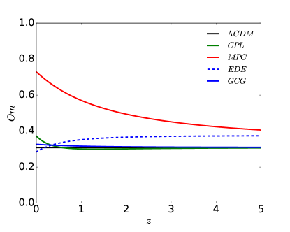
Applying the $Om(z)$ diagnostic to the cosmological models considered in our work, we can get the relation between the redshift and $Om(z)$ for different cosmological models, which is specifically presented in Fig. 7. The $Om(z)$ for the CPL and GCG models cannot be distinguished from each other as well as from $\rm{\Lambda}$CDM model. Moreover, the $Om(z)$ of CPL, GCG, EDE models cannot be distinguished at present time unless high-precision observations are obtained and applied. Another impressive feature of Fig.7 is that the $Om(z)$ for the MPC model, a cosmological candidate proposed without introducing dark energy in the Universe, absolutely deviates from the $\rm{\Lambda}$CDM model and other cosmological models.

Figure 8: The evolution of the statefinder pair $(r,s)$ for various cosmological models. The red point at $(r,s)\,=\,(0,1)$ represents $\rm{\Lambda}$CDM model and the diamond point on each curve means the present value of the statefinder pair $(r,s)$ for each cosmological model.

Figure 9: The evolution of the statefinder pair $(q,s)$ for the four cosmological models. The diamond point on each curve denotes the current value of $(q,s)$ for each cosmological model.

Apart from the $Om(z)$, the statefinder diagnostic, which has been extensively applied to discriminate different cosmological models, involves the third derivative of the scale factor $a$ as (sahni2003statefinder, )

$$r\,=\,\frac{\dddot{a}}{aH^{3}},\,\,\,\,\,\,s\,=\,\frac{r-1}{3(q-1/2)}$$ (23)

and one can plot the corresponding trajectories in the $r-s$ plane. For a certain cosmological model, the statefinder can be easily derived as

$$r(z)\,=\,1-2\frac{E^{\prime}(z)}{E(z)}(1+z)+[\frac{E^{\prime\prime}(z)}{E(z)}+(\frac{E^{\prime}(z)}{E(z)})^{2}](1+z)^{2}$$ (24)

and

$$s(z)\,=\,\frac{r(z)-1}{3(q(z)-1/2)}$$ (25)

where $E(z)\,=\,H(z)/H_{0}$ and the deceleration parameter $q(z)$ can be expressed as

$$q(z)\,=\,\frac{E^{\prime}(z)}{E(z)}(1+z)-1.$$ (26)

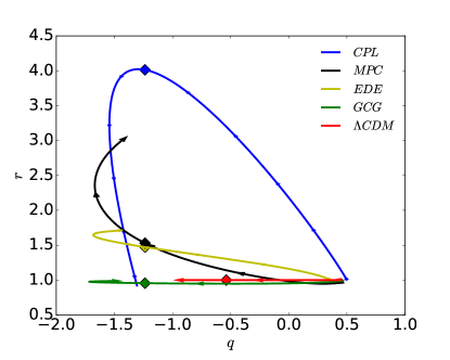
Applying the best fits from the joint analysis to each cosmological model, we obtain the evolution of the statefinder $(r,s)$ and the deceleration parameter $q$.

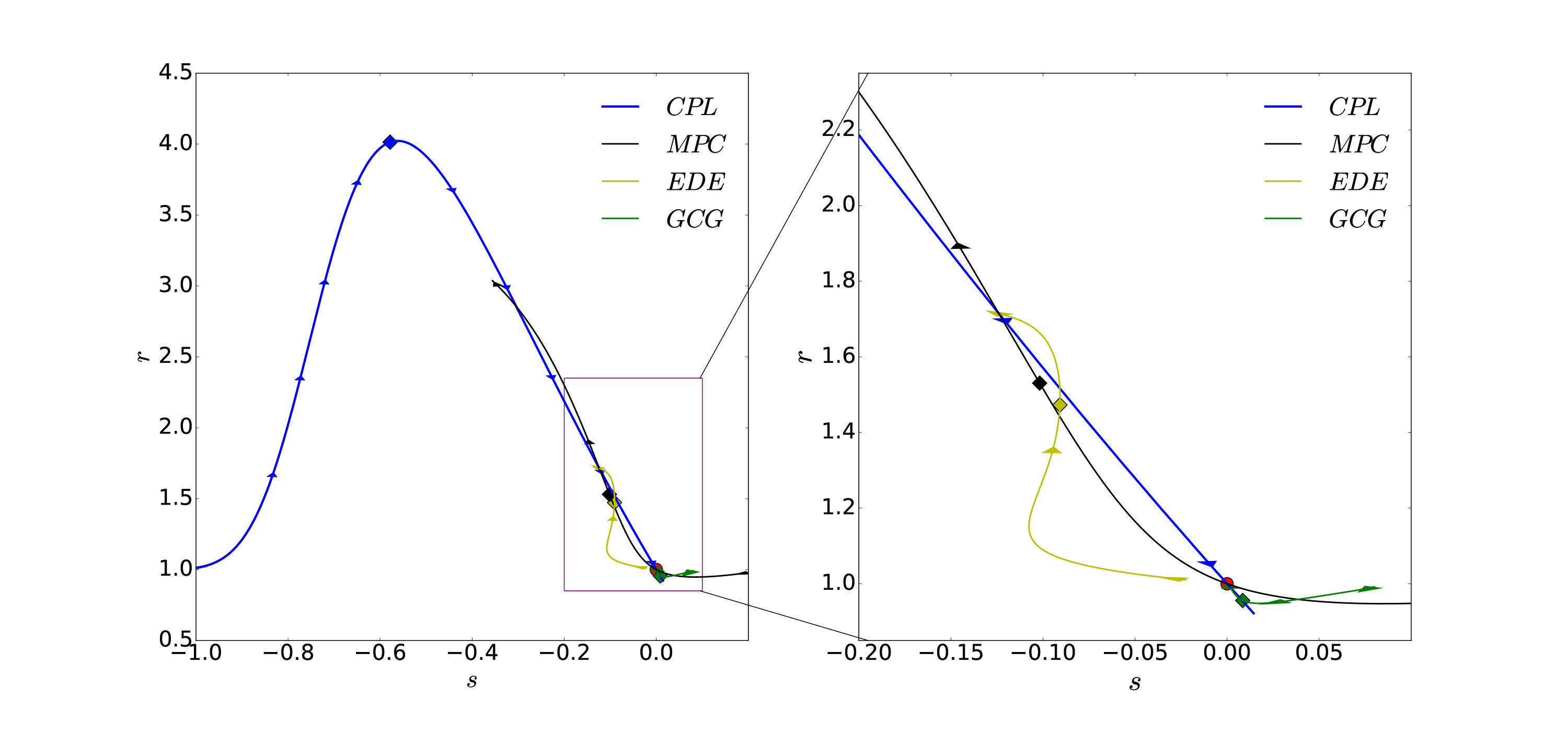
The evolution of the statefinder pair $(r,s)$ for different cosmological models is shown in Fig. 8. The red point at $(r,s)\,=\,(0,1)$ indicates the statefinder of $\rm{\Lambda}$CDM model and the diamond on each curve shows the present value of the statefinder $(r,s)$ for each cosmological model. It is apparent that the CPL model can be distinguished from other cosmological models at present time, however, it will approach $\rm{\Lambda}$CDM in the near future. Meanwhile, the MPC and EDE models, which are not distinguishable from each other by the statefinder, is deviating from $\rm{\Lambda}$CDM at the present epoch. More importantly, the GCG model exhibits very similar evolution tendency to the concordance cosmological constant.

The evolution trajectories in the $r-q$ plane are plotted in Fig. 9. For the four cosmological models considered in this analysis, we observe the signature flip from positive to negative in the value of $q$, which successfully explains the recent phase transition of these models. The diamond points on different curves in Fig. 9 denote the value of $q$ and $r$ at present time for different cosmological models. One can see the value of deceleration parameter $q$ is very close to each other at present time, which is quite different from the behavior of $r$. As for the evolution of cosmological models, at the present epoch, the GCG model and $\rm{\Lambda}$CDM model are not distinguishable and the MPC model can not be distinguished from EDE model. However, in the near future they will evolve diversely, which is in well consistent with the results obtained from the $r-s$ plot.

7 Conclusions

In this paper, we place constraints on four alternative cosmological models under the assumption of the spatial flatness of the Universe: Chevallier-Ploarski-Linder parametrization (CPL), Entropy Dark Energy model (EDE), General Chaplygin Gas model (GCG) and Modified Polytropic Cardassian model (MPC). A new compilation of 120 angular-size/redshift data compact radio quasars observed by very-long-baseline interferometry (VLBI), whose statistical linear sizes show negligible dependence on redshifts and intrinsic luminosity and thus represents standard rulers in cosmology, are used to test these cosmological models. Compared with BAO and galaxy clusters acting as cosmological standard rulers, higher-redshift radio-loud quasars are valuable additions to standard rulers used for cosmological tests and the inclusion of quasars could result in a fair coverage of redshifts, which enable QSO to be an excellent complement to other observational probes at lower redshifts.

Our results show that the constraints on CPL obtained from the quasar sample are well consistent with that obtained from BAO but in tension with that from galaxy clusters. Note that the concordance $\rm{\Lambda}$CDM cosmology ($w_{0}=-1$, $w_{a}=0$) is consistent with the quasar and BAO standard ruler data at less than 1$\sigma$ level. For other cosmological models considered, quasars provide fits in agreement with those obtained with other probes at $1\sigma$ level. Meanwhile, we have calculated the Figure of Merit for each cosmological model, which is explicitly summarized in Table 1. Out of all the candidate models considered, it is obvious that the QSO data could provide better statistically constraints on cosmological parameters than BAO. When taking the observations of galaxy cluster into consideration, quasars perform better than galaxy clusters in the framework of two cosmological models, GCG and EDE models. Based on the best-fits obtained with QSO+BAO+Cluster, we apply two model diagnostics, $Om(z)$ and statefinder to differentiate the dynamical behavior of the four cosmological models. On the one hand, the results from the $Om(z)$ diagnostic show that the CPL, GCG, EDE models cannot be distinguished at the present epoch. However, the MPC model, a cosmological candidate proposed without introducing dark energy in the Universe, absolutely deviates from the $\rm{\Lambda}$CDM model and other cosmological models. On the other hand, in the framework of statefinder diagnostics, MPC and EDE are will deviate from $\rm{\Lambda}$CDM model in the near future, while GCG model cannot be distinguished from $\rm{\Lambda}$CDM model unless much higher precision observations are available.

8 acknowledgments

This work was supported by the National Key Research and Development Program of China under Grants No. 2017YFA0402603; the Ministry of Science and Technology National Basic Science Program (Project 973) under Grants No. 2014CB845806; the National Natural Science Foundation of China under Grants Nos. 11503001, 11373014, and 11690023; the Fundamental Research Funds for the Central Universities and Scientific Research Foundation of Beijing Normal University; China Postdoctoral Science Foundation under grant No. 2015T80052; and the Opening Project of Key Laboratory of Computational Astrophysics, National Astronomical Observatories, Chinese Academy of Sciences. X.L. was supported by the China Scholarship Council. This research was also partly supported by the Poland-China Scientific & Technological Cooperation Committee Project No. 35-4. M.B. was supported by Foreign Talent Introducing Project and Special Fund Support of Foreign Knowledge Introducing Project in China.

References

- [1] Adam G Riess, Alexei V Filippenko, Peter Challis, Alejandro Clocchiatti, Alan Diercks, Peter M Garnavich, Ron L Gilliland, Craig J Hogan, Saurabh Jha, Robert P Kirshner, et al. Observational evidence from supernovae for an accelerating universe and a cosmological constant. The Astronomical Journal, 116(3):1009, 1998.
- [2] Adam G Riess, Louis-Gregory Strolger, Stefano Casertano, Henry C Ferguson, Bahram Mobasher, Ben Gold, Peter J Challis, Alexei V Filippenko, Saurabh Jha, Weidong Li, et al. New hubble space telescope discoveries of type ia supernovae at : narrowing constraints on the early behavior of dark energy. The Astrophysical Journal, 659(1):98, 2007.
- [3] N Suzuki, D Rubin, C Lidman, G Aldering, R Amanullah, K Barbary, LF Barrientos, J Botyanszki, M Brodwin, N Connolly, et al. The hubble space telescope cluster supernova survey. v. improving the dark-energy constraints above z¿ 1 and building an early-type-hosted supernova sample. The Astrophysical Journal, 746(1):85, 2012.
- [4] Will J Percival, Beth A Reid, Daniel J Eisenstein, Neta A Bahcall, Tamas Budavari, Joshua A Frieman, Masataka Fukugita, James E Gunn, Željko Ivezić, Gillian R Knapp, et al. Baryon acoustic oscillations in the sloan digital sky survey data release 7 galaxy sample. Monthly Notices of the Royal Astronomical Society, 401(4):2148–2168, 2010.
- [5] David N Spergel, Licia Verde, Hiranya V Peiris, E Komatsu, MR Nolta, CL Bennett, M Halpern, G Hinshaw, N Jarosik, A Kogut, et al. First-year wilkinson microwave anisotropy probe (wmap)* observations: determination of cosmological parameters. The Astrophysical Journal Supplement Series, 148(1):175, 2003.
- [6] Eiichiro Komatsu, KM Smith, J Dunkley, CL Bennett, B Gold, G Hinshaw, N Jarosik, D Larson, MR Nolta, L Page, et al. Seven-year wilkinson microwave anisotropy probe (wmap*) observations: cosmological interpretation. The Astrophysical Journal Supplement Series, 192(2):18, 2011.
- [7] Gary Hinshaw, D Larson, Eiichiro Komatsu, DN Spergel, CL Bennett, J Dunkley, MR Nolta, M Halpern, RS Hill, N Odegard, et al. Nine-year wilkinson microwave anisotropy probe (wmap) observations: cosmological parameter results. The Astrophysical Journal Supplement Series, 208(2):19, 2013.
- [8] PAR Ade, N Aghanim, M Arnaud, M Ashdown, J Aumont, C Baccigalupi, AJ Banday, RB Barreiro, JG Bartlett, N Bartolo, et al. Planck 2015 results-xiii. cosmological parameters. Astronomy & Astrophysics, 594:A13, 2016.
- [9] Shuo Cao, Zonghong Zhu, and Ren Zhao. Testing and selecting dark energy models with lens redshift data. Physical Review D, 84(2), 2011.
- [10] Xiao-Lei Li, Shuo Cao, Xiao-Gang Zheng, Song Li, and Marek Biesiada. Comparison of cosmological models using standard rulers and candles. Research in Astronomy and Astrophysics, 16(5):015, 2016.
- [11] Steven Weinberg. The cosmological constant problem. Reviews of modern physics, 61(1):1, 1989.
- [12] Bharat Ratra and Philip JE Peebles. Cosmological consequences of a rolling homogeneous scalar field. Physical Review D, 37(12):3406, 1988.
- [13] PJE Peebles and Bharat Ratra. Cosmology with a time-variable cosmological’constant’. The Astrophysical Journal, 325:L17–L20, 1988.
- [14] Robert R Caldwell. A phantom menace? cosmological consequences of a dark energy component with super-negative equation of state. Physics Letters B, 545(1):23–29, 2002.
- [15] Michel Chevallier and David Polarski. Accelerating universes with scaling dark matter. International Journal of Modern Physics D, 10(02):213–223, 2001.
- [16] Eric V Linder. Cosmic shear with next generation redshift surveys as a cosmological probe. Physical Review D, 68(8):083503, 2003.
- [17] Shuo Cao and Zong-Hong Zhu. Cosmic equation of state from combined angular diameter distances: Does the tension with luminosity distances exist? Physical Review D, 90(8):083006, 2014.
- [18] Gabriela Caldera-Cabral, Roy Maartens, and L Arturo Urena-Lopez. Dynamics of interacting dark energy. Physical Review D, 79(6):063518, 2009.
- [19] Jussi Väliviita, Roy Maartens, and Elisabetta Majerotto. Observational constraints on an interacting dark energy model. Monthly Notices of the Royal Astronomical Society, 402(4):2355–2368, 2010.
- [20] Xiaogang Zheng, Marek Biesiada, Shuo Cao, Jingzhao Qi, and Zong-Hong Zhu. Ultra-compact structure in radio quasars as a cosmological probe: a revised study of the interaction between cosmic dark sectors. arXiv preprint arXiv:1705.06204, 2017.
- [21] Alexander Kamenshchik, Ugo Moschella, and Vincent Pasquier. An alternative to quintessence. Physics Letters B, 511(2):265–268, 2001.
- [22] T Barreiro, O Bertolami, and P Torres. Wmap five-year data constraints on the unified model of dark energy and dark matter. Physical Review D, 78(4):043530, 2008.
- [23] Qing-Guo Huang and Miao Li. The holographic dark energy in a non-flat universe. Journal of Cosmology and Astroparticle Physics, 2004(08):013, 2004.
- [24] MR Setare. The holographic dark energy in non-flat brans–dicke cosmology. Physics Letters B, 644(2):99–103, 2007.
- [25] Ahmad Sheykhi and Mubasher Jamil. Interacting hde and nade in brans–dicke chameleon cosmology. Physics Letters B, 694(4):284–288, 2011.
- [26] Katherine Freese and Matthew Lewis. Cardassian expansion: a model in which the universe is flat, matter dominated, and accelerating. Physics Letters B, 540(1):1–8, 2002.
- [27] Jing-Zhao Qi, Shuo Cao, Marek Biesiada, Xiaogang Zheng, and Zong-Hong Zhu. New observational constraints on cosmology from radio quasars. Eur. Phys. J. C, 77:502, 2017.
- [28] Tengpeng Xu, Shuo Cao, Qi Jing-Zhao, Biesiada Marek, Zheng Xiaogang, and Zhu Zong-Hong. A new test of gravity with the cosmological standard rulers in radio quasars. Eur. Phys. J. C, submitted, 2017.
- [29] Shuo Cao, Yu Pan, Marek Biesiada, Wlodzimierz Godlowski, and Zonghong Zhu. Constraints on cosmological models from strong gravitational lensing systems. Journal of Cosmology and Astroparticle Physics, 2012(03):016–016, 2011.
- [30] Shuo Cao, Marek Biesiada, Raphael Gavazzi, Aleksandra Piorkowska, and Zonghong Zhu. Cosmology with strong lensing systems. The Astrophysical Journal, 806(2):185, 2015.
- [31] Ari Buchalter, David J Helfand, Robert H Becker, and Richard L White. Constraining 0 with the angular size-redshift relation of double-lobed quasars in the first survey. The Astrophysical Journal, 494(2):503, 1998.
- [32] LI Gurvits, KI Kellermann, and S Frey. The“angular size-redshift”relation for compact radio structures in quasars and radio galaxies. arXiv preprint astro-ph/9812018, 1998.
- [33] Ruth A Daly and SG Djorgovski. A model-independent determination of the expansion and acceleration rates of the universe as a function of redshift and constraints on dark energy. The Astrophysical Journal, 597(1):9, 2003.
- [34] D Watson, KD Denney, Marianne Vestergaard, and Tamara Maree Davis. A new cosmological distance measure using active galactic nuclei. The Astrophysical Journal Letters, 740(2):L49, 2011.
- [35] Jian-Min Wang, Pu Du, David Valls-Gabaud, Chen Hu, and Hagai Netzer. Super-eddington accreting massive black holes as long-lived cosmological standards. Physical Review Letters, 110(8):081301, 2013.
- [36] Paola Marziani and Jack W Sulentic. Highly accreting quasars: sample definition and possible cosmological implications. Monthly Notices of the Royal Astronomical Society, 442(2):1211–1229, 2014.
- [37] Guido Risaliti and Elisabeta Lusso. A hubble diagram for quasars. The Astrophysical Journal, 815(1):33, 2015.
- [38] Shuo Cao, Marek Biesiada, John Jackson, Xiaogang Zheng, Yuhang Zhao, and Zong-Hong Zhu. Measuring the speed of light with ultra-compact radio quasars. Journal of Cosmology and Astroparticle Physics, 2017(02):012, 2017.
- [39] Shuo Cao, Xiaogang Zheng, Marek Biesiada, Jingzhao Qi, Yun Chen, and Zong-Hong Zhu. Ultra-compact structure in intermediate-luminosity radio quasars: building a sample of standard cosmological rulers and improving the dark energy constraints up to . Astronomy and Astrophysics, in press, doi:10.1051/0004-6361/201730551, 2017.
- [40] Massimiliano Bonamente, Marshall K Joy, Samuel J LaRoque, John E Carlstrom, Erik D Reese, and Kyle S Dawson. Determination of the cosmic distance scale from sunyaev-zel’dovich effect and chandra x-ray measurements of high-redshift galaxy clusters. The Astrophysical Journal, 647(1):25, 2006.
- [41] Varun Sahni, Arman Shafieloo, and Alexei A Starobinsky. Two new diagnostics of dark energy. Physical Review D, 78(10):103502, 2008.
- [42] Varun Sahni, Tarun Deep Saini, Alexei A Starobinsky, and Ujjaini Alam. Statefinder—a new geometrical diagnostic of dark energy. JETP Letters, 77(5):201–206, 2003.
- [43] Florian Beutler, Chris Blake, Matthew Colless, D Heath Jones, Lister Staveley-Smith, Lachlan Campbell, Quentin Parker, Will Saunders, and Fred Watson. The 6df galaxy survey: baryon acoustic oscillations and the local hubble constant. Monthly Notices of the Royal Astronomical Society, 416(4):3017–3032, 2011.
- [44] Nikhil Padmanabhan, Xiaoying Xu, Daniel J Eisenstein, Richard Scalzo, Antonio J Cuesta, Kushal T Mehta, and Eyal Kazin. A 2 per cent distance to by reconstructing baryon acoustic oscillations–i. methods and application to the sloan digital sky survey. Monthly Notices of the Royal Astronomical Society, 427(3):2132–2145, 2012.
- [45] Lauren Anderson, Eric Aubourg, Stephen Bailey, Dmitry Bizyaev, Michael Blanton, Adam S Bolton, J Brinkmann, Joel R Brownstein, Angela Burden, Antonio J Cuesta, et al. The clustering of galaxies in the sdss-iii baryon oscillation spectroscopic survey: baryon acoustic oscillations in the data release 9 spectroscopic galaxy sample. Monthly Notices of the Royal Astronomical Society, 427(4):3435–3467, 2012.
- [46] Chris Blake, Sarah Brough, Matthew Colless, Carlos Contreras, Warrick Couch, Scott Croom, Darren Croton, Tamara M Davis, Michael J Drinkwater, Karl Forster, et al. The wigglez dark energy survey: Joint measurements of the expansion and growth history at z¡ 1. Monthly Notices of the Royal Astronomical Society, 425(1):405–414, 2012.
- [47] Rahman Amanullah, Chris Lidman, D Rubin, G Aldering, P Astier, K Barbary, MS Burns, A Conley, KS Dawson, SE Deustua, et al. Spectra and light curves of six type ia supernovae at and the union2 compilation. The Astrophysical Journal, 716(1):712, 2010.
- [48] Damien A Easson, Paul H Frampton, and George F Smoot. Entropic accelerating universe. Physics Letters B, 696(3):273–277, 2011.
- [49] Damien A Easson, Paul H Frampton, and George F Smoot. Entropic inflation. International Journal of Modern Physics A, 27(12):1250066, 2012.
- [50] Jianbo Lu, Yuanxing Gui, and Li Xin Xu. Observational constraint on generalized chaplygin gas model. The European Physical Journal C-Particles and Fields, 63(3):349–354, 2009.
- [51] Paolo Gondolo and Katherine Freese. An accelerating universe from dark matter interactions with negative pressure. arXiv preprint hep-ph/0211397, 2002.
- [52] R. D. Blandford and M. J. Rees. Some comments on radiation mechanisms in lacertids. pages 328–341, 01 1978.
- [53] J D Silverman, K Kovac, C Knobel, S J Lilly, M Bolzonella, F Lamareille, V Mainieri, M Brusa, N Cappelluti, Y Peng, et al. The environments of active galactic nuclei within the zcosmos density field. The Astrophysical Journal, 695(1):171–182, 2009.
- [54] Philip F Hopkins and Eliot Quataert. How do massive black holes get their gas. Monthly Notices of the Royal Astronomical Society, 407(3):1529–1564, 2009.
- [55] A B Pushkarev and Y Y Kovalev. Milky way scattering properties and intrinsic sizes of active galactic nuclei cores probed by very long baseline interferometry surveys of compact extragalactic radio sources. Monthly Notices of the Royal Astronomical Society, 452(4):4274–4282, 2015.
- [56] Cao Shuo, Biesiada Marek, Zheng Xiaogang, Qi Jing-Zhao, Tengpeng Xu, and Zhu Zong-Hong. Cosmological application of multi-frequency vlbi observations of ultra-compact structure in radio quasars. The Astrophysical Journal, submitted, 2017.
- [57] Shuo Cao, Nan Liang, and Zonghong Zhu. Testing the phenomenological interacting dark energy with observational data. Monthly Notices of the Royal Astronomical Society, 416(2):1099–1104, 2010.
- [58] Shuo Cao and Zonghong Zhu. Constraints on cosmological models from lens redshift data. Astronomy and Astrophysics, 538, 2011.
- [59] Daniel J Eisenstein and Wayne Hu. Baryonic features in the matter transfer function. The Astrophysical Journal, 496(2):605, 1998.
- [60] Michael J Mortonson, Dragan Huterer, and Wayne Hu. Figures of merit for present and future dark energy probes. Physical Review D, 82(6):063004, 2010.
- [61] Shuo Cao, G Covone, and Zonghong Zhu. Testing the dark energy with gravitational lensing statistics. The Astrophysical Journal, 755(1):31, 2012.
- [62] Titus K Mathew, Chinthak Murali, and J Shejeelammal. Evolution of non-interacting entropic dark energy and its phantom nature. Modern Physics Letters A, 31(12):1650071, 2016.
- [63] Z-H Zhu. Generalized chaplygin gas as a unified scenario of dark matter/energy: Observational constraints. Astronomy & Astrophysics, 423(2):421–426, (2004).
- [64] Puxun Wu and Hongwei Yu. Generalized chaplygin gas model: constraints from hubble parameter versus redshift data. Physics Letters B, 644(1):16–19, 2007.
- [65] JS Alcaniz, Abha Dev, and Deepak Jain. Constraints on the cardassian expansion from the cosmic lens all-sky survey gravitational lens statistics. The Astrophysical Journal, 627(1):26, 2005.
- [66] Chao-Jun Feng and Xin-Zhou Li. Cardassian universe constrained by latest observations. Physics Letters B, 692(2):152–156, 2010.
- [67] Nan Liang, Pu-Xun Wu, and Zong-Hong Zhu. Latest cosmological constraints on cardassian expansion models including the updated gamma-ray bursts. Research in Astronomy and Astrophysics, 11(9):1019, 2011.
- [68] Zhengxiang Li, Puxun Wu, and Hongwei Yu. Testing nonstandard cosmological models with snls3 supernova data and other cosmological probes. The Astrophysical Journal, 744(2):176, 2011.
- [69] Juan Magaña, V Motta, T Verdugo, Eric Jullo, et al. A magnified glance into the dark sector: probing cosmological models with strong lensing in a1689. The Astrophysical Journal, 813(1):69, 2015.
- [70] Andreas Albrecht, Gary Bernstein, Robert Cahn, Wendy L Freedman, Jacqueline Hewitt, Wayne Hu, John Huth, Marc Kamionkowski, Edward W Kolb, Lloyd Knox, et al. Report of the dark energy task force. arXiv preprint astro-ph/0609591, 2006.
- [71] Yun Wang. Figure of merit for dark energy constraints from current observational data. Physical Review D, 77(12):123525, 2008.
- [72] Xuheng Ding, Marek Biesiada, Shuo Cao, Zhengxiang Li, and Zonghong Zhu. Is there evidence for dark energy evolution. The Astrophysical Journal, 803(2), 2015.
- [73] Xiaogang Zheng, Xuheng Ding, Marek Biesiada, Shuo Cao, and Zonghong Zhu. What are and diagnostics telling us in light of data? The Astrophysical Journal, 825(1):17, 2016.