The effect of population abundances on the stability of large random ecosystems

Abstract

Random matrix theory successfully connects the structure of interactions of large ecological communities to their ability to respond to perturbations. One of the most debated aspects of this approach is the missing role of population abundances. Despite being one of the most studied patterns in ecology, and one of the most empirically accessible quantities, population abundances are always neglected in random matrix approaches and their role in determining stability is still not understood. Here, we tackle this question by explicitly including population abundances in a random matrix framework. We obtain an analytical formula that describes the spectrum of a large community matrix for arbitrary feasible species abundance distributions. The emerging picture is remarkably simple: while population abundances affect the rate to return to equilibrium after a perturbation, the stability of large ecosystems is uniquely determined by the interaction matrix. We confirm this result by showing that the likelihood of having a feasible and unstable solution in the Lotka-Volterra system of equations decreases exponentially with the number of species for stable interaction matrices.

I Introduction

Since the work of Lotka and Volterra, ecologists have attempted to mathematize the interactions between populations to build predictive models of population dynamics. This is a complex problem – ecological communities are often composed of a large number of species May1988 ; May1988 , the equations describing their interactions have been debated for decades Arditi2012 , and the estimation of parameters and initial conditions is often unfeasible from an empirical standpoint.

To circumvent this problem, Robert May May1972 introduced the idea of modeling complex ecological communities using random matrices. Consider the case in which the dynamics of the populations can be described by a system of ordinary differential equations:

$$\frac{dx_{i}(t)}{dt}=f_{i}(\boldsymbol{x}(t)),$$ (1)

where $\boldsymbol{x}(t)$ is a vector containing the populations abundances at time $t$, and the function $f_{i}$ relates the abundance of all populations to the growth of population $i$. In general, $f_{i}$ is a nonlinear equation with several parameters.

Suppose that the system admits a feasible equilibrium point, i.e., a vector $\boldsymbol{x}^{\ast}$ such that $f_{i}(\boldsymbol{x}^{\ast})=0$ and $x_{i}^{\ast}>0$ for all $i$. If we start the system at this point, it will remain there indefinitely. We can therefore ask whether the system will go back to the equilibrium, or rather move away from it, following a perturbation. This type of stability analysis can be carried out by building the Jacobian matrix $J_{ij}=\partial f_{i}(\boldsymbol{x}(t))/\partial x_{j}$ and evaluating it at the equilibrium point, yielding the so-called community matrix $\boldsymbol{M}=\left.\boldsymbol{J}\right\rvert_{\boldsymbol{x}^{\ast}}$. If all the eigenvalues of $\boldsymbol{M}$ have negative real part, then the equilibrium is locally asymptotically stable, and the system will return to it after sufficiently small perturbations; if any of the eigenvalues have a positive real part, the system will move away from the equilibrium when perturbed.

Clearly, to build $\boldsymbol{M}$ one would need to precisely know the functions $f_{i}$, as well as their parameters, and solve for the equilibrium (or equilibria) $\boldsymbol{x}^{\ast}$. May took a radically different approach and analyzed the case in which $\boldsymbol{M}$ is a random matrix with independent, identically distributed off-diagonal elements, and constant diagonal elements May1972 . For this parameterization, he was able to show that the community matrices describing sufficiently large and complex ecological communities are always unstable. The random-matrix approach was recently extended and refined to include different types of interaction between the populations Allesina2012 ; ReviewRMT , as well as to study the effect of more complex network structures, such as the hierarchical organization of food-webs Allesina2015a and the modular pattern often displayed by biological networks Grilli2016 .

By modeling directly the matrix $\boldsymbol{M}$ as a random matrix, one does not require a precise characterization of the functions $f_{i}$ and the equilibrium $\boldsymbol{x}^{\ast}$. While mathematically convenient, this approach does not explicitly take into account the abundance of the populations—a type of data that is empirically much more accessible than interaction coefficients or the elements of the community matrix.

The distribution of species abundances (SAD) has been shown to have remarkably similar features across different species rich communities Bell2001a with a skewed shape and few highly abundant species. The log-series distribution Fisher1943a , discrete lognormal Preston1948 and negative binomial Volkov2007 have all been proposed to describe empirical SADs, and have been shown to emerge from either neutral Caswell1976 ; Hubbell2001a ; Volkov2003 ; Azaele2016 or niche mechanisms MacArthur1957a ; Vandermeer1966 .

The role of species abundances in structuring the community matrix $\boldsymbol{M}$ can be easily seen by considering one of the simplest models of population dynamics, the Generalized Lotka-Volterra (GLV) model:

$$\frac{dx_{i}(t)}{dt}=x_{i}(t)\left(r_{i}+\sum_{j}A_{ij}x_{j}(t)\right)\ ,$$ (2)

where $r_{i}$ is the intrinsic growth rate of species $i$, and $A_{ij}$ is the per-capita effect of species $j$ on the growth of $i$. If a feasible equilibrium (i.e., one where all species have positive abundance) exists, then it can be found solving the system of equations

$$0=r_{i}+\sum_{j}A_{ij}x^{\ast}_{j}\ ,$$ (3)

yielding the community matrix $M_{ij}=A_{ij}x_{i}^{\ast}$, which can be written in matrix form as

$$\boldsymbol{M}=\boldsymbol{X}\boldsymbol{A}\ ,$$ (4)

where $\boldsymbol{X}$ is a diagonal matrix with $X_{ii}=x_{i}^{\ast}$ and zeros elsewhere. Even if the elements of $\boldsymbol{A}$ were independent, identically distributed samples from a distribution, the elements of $\boldsymbol{M}$ would not be—the matrix of abundances $\boldsymbol{X}$ couples all the coefficients in the same row, such that the distribution of the elements in each row would in principle be different.

One of the main goals of this work is to extend the random matrix approach by considering a random matrix of abundances $\boldsymbol{X}$ and a random matrix of interactions $\boldsymbol{A}$, and determining the stability of $\boldsymbol{M}$ under these conditions. In this way, we address the effect of species abundances on stability, thereby lifting one of the main criticisms of the random matrix approach ReviewRMT ; amnatjames ; Jacquet2016 .

As we stated above when analyzing coexistence, we need population abundances to be positive (feasible). Stability cannot, at least in principle, be disentangled from the constraint imposed by feasibility on interactions Roberts1974 . Diversity and interaction properties have important consequences for the range of parameters corresponding to feasible solutions Rohr2014 ; Stone2016 ; Grilli2017 . While the interest in feasibility has grown considerably in recent years, the relationship between feasibility and stability is still unclear. In fact, most of the studies on feasibility assume strong conditions on the interaction matrix (e.g., D-stability, diagonal stability) that guarantee stability of any feasible solution Rohr2014 ; Grilli2017 . It is still unclear when these assumptions are justified and how likely it is for large random interaction matrices to meet these conditions.

In the second part of this work, we focus on the relationship between feasibility and stability. In particular, we study the relationship between the stability of $\boldsymbol{A}$ and that of $\boldsymbol{M}$ for the GLV model. Our results show that, given a stable random matrix $\boldsymbol{A}$, the probability that an arbitrary feasible equilibrium is unstable decreases exponentially with diversity. This result strongly suggests that, provided that the interaction matrix $\boldsymbol{A}$ is stable, feasible solutions are almost surely stable. We therefore provide a more robust justification to both May’s original paper—by showing that population abundances do not affect qualitatively stability—and the more recent work on feasibility that assumes stability—by predicting that this assumption is almost surely met for large random systems.

II Constructing the community matrix with arbitrary population abundance

We consider a system of $S$ interacting populations whose dynamics are described by the GLV model in equation 2, assume that a feasible equilibrium $\boldsymbol{x}^{\ast}$ exists, and define $\boldsymbol{X}$ as the diagonal matrix with diagonal entries $X_{ii}=x^{\ast}_{i}$. The feasible fixed point $\boldsymbol{x}^{\ast}$ is locally asymptotically stable if and only if all the eigenvalues of the community matrix $\boldsymbol{M}=\boldsymbol{X}\boldsymbol{A}$, with components $M_{ij}=x^{\ast}_{j}A_{ij}$, have a negative real part. Here, we model $\boldsymbol{A}$ as a random matrix and $\boldsymbol{x}^{\ast}$ as a random vector with positive components, with the goal of studying the spectrum (distribution of the eigenvalues) of the community matrix $\boldsymbol{M}$ . From the GLV model, specifiying a feasible fixed point $\boldsymbol{X}^{\ast}$ is the same as specifying a vector of intrinsic growth rates $\boldsymbol{r}$ inside the feasibility domain Rohr2014 ; Grilli2017 .

More specifically, we assume that the diagonal entries of the diagonal matrix $\boldsymbol{X}$ are drawn from an arbitrary distribution with positive support, mean $\mu_{X}$, and variance $\sigma_{X}^{2}$. The diagonal entries of $\boldsymbol{A}$ are drawn from an arbitrary distribution with support in the negative axis, mean $\mu_{d}$, and variance $\sigma_{d}^{2}$. Finally, each off-diagonal pair $(A_{ij},A_{ji})$ in $\boldsymbol{A}$ is drawn independently from a bivariate distribution with identical marginal means $\mu$, variances $\sigma^{2}$, and correlation $\rho$. Unless otherwise specified, we focus on the case $\sigma_{d}=0$, while we discuss in the Supplementary Information the effects of variability in self-regulation.

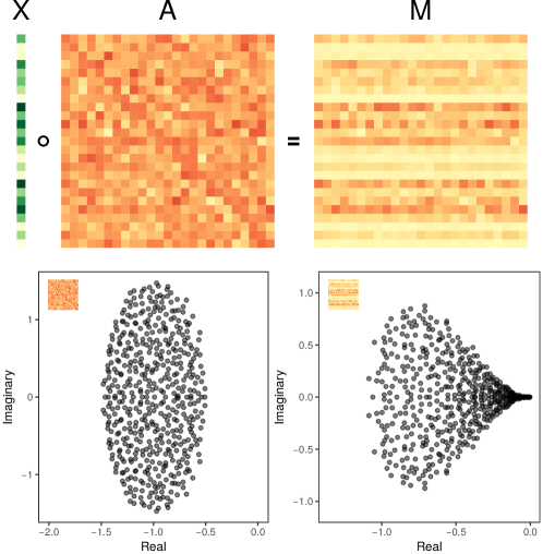
In the case of $\sigma_{d}=0$ and in the limit of large $S$, the spectrum of $\boldsymbol{A}$ is known and is independent of the choice of the bivariate distribution (provided that mild conditions on the finiteness of the moments are satisfied nguyen2012elliptic ). In particular, $\boldsymbol{A}$ has one eigenvalue equal to $-\mu_{d}+S\mu$ ORourke2014 , while the others (the bulk of eigenvalues) are uniformly distributed in an ellipse in the complex plane centered in $-\mu_{d}-\mu$ with horizontal axis $\sqrt{S}\sigma(1+\rho)$ and vertical axis $\sqrt{S}\sigma(1-\rho)$ nguyen2012elliptic ; Allesina2012 ; ORourke2014 . Figure 1 shows an example of the spectrum of $\boldsymbol{A}$.

Figure 1 also shows an example of the eigenvalues of the community matrix $\boldsymbol{M}=\boldsymbol{X}\boldsymbol{A}$ where the diagonal entries of $\boldsymbol{X}$ are independent random variables drawn from a uniform distribution. It is evident that the bulk of eigenvalues of $\boldsymbol{M}$ does not follow the elliptic law.

Figure 1: The top row shows the vector of abundances $\boldsymbol{x}^{\ast}$, the interaction matrix $\boldsymbol{A}$ and the community matrix $\boldsymbol{M}=\boldsymbol{X}\boldsymbol{A}$ (where $\boldsymbol{X}$ is a diagonal matrix with diagonal entries $\boldsymbol{x}^{\ast}$), with colors from red (negative) to green (positive). The bottom row shows the eigenvalues of $\boldsymbol{A}$ and $\boldsymbol{M}$, for $S=500$. The diagonal entries of $\boldsymbol{X}$ are sampled from a uniform distribution on $[0,1]$, and matrix $\boldsymbol{A}$ is built sampling independently each pair $(A_{ij},A_{ji})$ from a normal bivariate distribution with identical marginals defined by $\mu=0$, $\sigma=1/\sqrt{S}$, and correlation $\rho=-0.5$. The diagonal elements of $\boldsymbol{A}$ are fixed at -1. The main goal of this work is to characterize the spectrum of $\boldsymbol{M}$ given the properties of $\boldsymbol{A}$ and $\boldsymbol{X}$.

III Disentangling the effect of the mean interaction strength

When the mean $\mu$ of the off-diagonal elements of the interaction matrix $\boldsymbol{A}$ does not equal zero, the spectra of $\boldsymbol{A}$ and $\boldsymbol{M}$ are characterized by the presence of an outlier. The value of this eigenvalue for the matrix $\boldsymbol{A}$ is known for the case $\sigma_{d}=0$, and in the limit of large $S$ ORourke2014 . It can be obtained by decomposing the matrix $\boldsymbol{A}$ as a sum of three matrices

$$\boldsymbol{A}=(\mu_{d}-\mu)\boldsymbol{I}+\mu\boldsymbol{1}+\boldsymbol{B}\ ,$$ (5)

where $\boldsymbol{I}$ is the identity matrix, $\boldsymbol{1}$ is a matrix of ones, and $\boldsymbol{B}$ is a random matrix with mean zero that follows the elliptic law. It has been proved ORourke2014 that the spectrum of $\boldsymbol{A}$ is characterized by a bulk of eigenvalues, determined by the spectrum of $(\mu_{d}-\mu)\boldsymbol{I}+\boldsymbol{B}$, and the presence of an outlier, whose value is (approximately) given by the largest eigenvalue of $(\mu_{d}-\mu)\boldsymbol{I}+\mu\boldsymbol{1}$, which has value $\mu_{d}+(S-1)\mu$.

Figure 2 shows that, if $\mu\neq 0$, the spectrum of $\boldsymbol{M}$ is also characterized by the presence of a bulk and of an outlying eigenvalue. By decomposing the matrix $\boldsymbol{M}$ as

$$\boldsymbol{M}=\boldsymbol{X}\left((\mu_{d}-\mu)\boldsymbol{I}+\mu\boldsymbol{1}+\boldsymbol{B}\right)\ ,$$ (6)

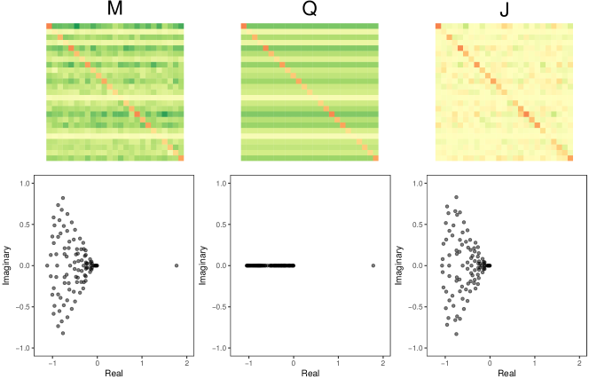
we show in the Supplementary Information that the bulk of the spectrum of $\boldsymbol{M}$ is determined by the eigenvalues of the matrix $\boldsymbol{J}=\boldsymbol{X}\left((\mu_{d}-\mu)\boldsymbol{I}+\boldsymbol{B}\right)$ and the outlier is given by largest eigenvalue of $\boldsymbol{Q}=\boldsymbol{X}\left((\mu_{d}-\mu)\boldsymbol{I}+\mu\boldsymbol{1}\right)$. Figure 2 shows an example of this decomposition, where it is evident that the bulks of eigenvalues of $\boldsymbol{M}$ and $\boldsymbol{J}$ are the same, and the outliers of $\boldsymbol{M}$ and $\boldsymbol{Q}$ match.

Figure 2: The top row shows the three matrices $\bf{M}$, $\bf{Q}$ and $\bf{J}$. The community matrix $\boldsymbol{M}=\boldsymbol{X}\boldsymbol{A}$, is obtained from the interaction matrix $\boldsymbol{A}$ that, without loss of generality, can be written as $\boldsymbol{A}=(\mu_{d}-\mu)\boldsymbol{I}+\mu\boldsymbol{1}+\boldsymbol{B}$, where $\boldsymbol{1}$ is a matrix of ones and $\boldsymbol{B}$ is a random matrix with diagonal elements fixed at zero whose coefficients have mean zero and variance $\sigma^{2}$. We define $\boldsymbol{Q}=\boldsymbol{X}((\mu_{d}-\mu)\boldsymbol{I}+\mu\boldsymbol{1})$ and $\boldsymbol{J}=\boldsymbol{X}(\mu_{d}\boldsymbol{I}+\boldsymbol{B})$. Equivalently, $\boldsymbol{Q}$ is the matrix with the same parameters as $\boldsymbol{M}$ except with $\sigma=0$, and $\boldsymbol{J}$ is obtained from the same parameters as $\boldsymbol{M}$ except with $\mu=0$ for the off-diagonal terms. Remarkably, the eigenvalues of $\boldsymbol{M}$, $\boldsymbol{J}$ and $\boldsymbol{Q}$ are simply related: the bulk of eigenvalues of $\boldsymbol{J}$ and that of $\boldsymbol{M}$ are the same, while the outlier of $\boldsymbol{M}$ is the same as that of $\boldsymbol{Q}$. This decomposition allows us to obtain an analytical prediction for the outlier, and in the Supplementary Information we find the spectrum of $\boldsymbol{Q}$ analytically. In the figure, we set $S=500$. The diagonal entries of $\boldsymbol{X}$ are sampled from a uniform distribution on $[0,1]$. $\boldsymbol{A}$ is sampled from a normal bivariate distribution with identical marginals $\mu=5/S$, $\sigma=5/\sqrt{S}$ and correlation $\rho=-0.5$.

The trace of $\boldsymbol{M}$ is given by

$$\operatorname*{\text{tr}}\left(\boldsymbol{M}\right)=\lambda_{\textrm{out}}+(S-1)\langle\lambda\rangle_{\textrm{bulk}}\ ,$$ (7)

where $\lambda_{\textrm{out}}$ is the value of the outlier and $\langle\lambda\rangle_{\textrm{bulk}}$ is the average eigenvalue in the bulk. Since the bulks of the eigenvalues of $\boldsymbol{M}$ and $\boldsymbol{J}$ are the same, we have that

$$\langle\lambda\rangle_{\textrm{bulk}}=\frac{1}{S}\operatorname*{\text{tr}}\left(\boldsymbol{J}\right)=\mu_{X}\left(\mu_{d}-\mu\right)\ .$$ (8)

Using the fact that

$$\operatorname*{\text{tr}}\left(\boldsymbol{M}\right)=S\mu_{d}\mu_{X}\ ,$$ (9)

we see that the outlier is equal to

$$\lambda_{\textrm{out}}=\mu_{X}\left(\mu_{d}+(S-1)\mu\right)\ .$$ (10)

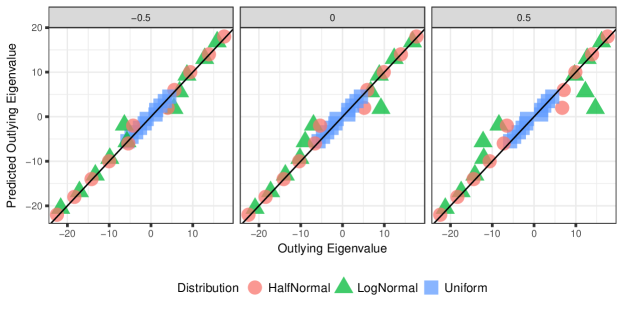
Figure 3 shows that this analytical prediction closely matches the outlier of the spectrum of $\boldsymbol{M}$.

Figure 3: The three panels show that our analytical prediction (equation 3) correctly matches the outlier of the spectrum, for different values of $\rho$ and population abundance distributions. The matrix $\boldsymbol{A}$ is built independently sampling the coefficients from a normal bivariate distribution with identical marginals defined by $\mu$, $\sigma$, and $\rho$. Here, we set $S=1000$ and $\sigma=1/\sqrt{S}$, and vary $\mu$ between $-10$ and $10$ to test our prediction. We draw $\boldsymbol{X}$ from three different distributions with positive support: uniform (on [0,1]), log-normal (with mean log-mean $0.5$ and log-standard deviation $0.5$) and half-normal (shifted rightwards to have support $(1,\infty)$, and with parameter $\theta=1$). We can observe deviations from our prediction when $\mu$ is small, especially when $\boldsymbol{X}$ is drawn from a log-normal distribution. This is because the eigenvalue corresponding to equation 10 is now contained in the bulk.

IV Analytical solution in the case $\rho=0$

In section III we showed that the spectrum of $\boldsymbol{M}$ is characterized by a bulk of eigenvalues and an outlier, which is determined by the mean of interaction matrix $\mu$. In the following, we focus on the bulk of eigenvalues, so we assume $\mu=0$.

Using the cavity method Rogers2008 ; Rogers2009 ; Grilli2016 , we derive in the Supplementary Information a system of equations for the spectral density of the matrix $\boldsymbol{M}$. These equations cannot be explicitly solved in the most general case, but they take a particularly simple form in the case where the correlation $\rho=0$. In this case, it is possible to write an implicit equation for the support of the spectrum, which takes the form

$$\int{\operatorname*{\text{d}}}x\ {\operatorname*{\text{d}}}s\ P_{XD}(x,s)\ \frac{Sx^{2}\sigma^{2}}{|\lambda-sx|^{2}}=1\ ,$$ (11)

where $P_{XD}(x,s)$ is the joint distribution of the population abundances $x$, with mean $\mu_{X}$ and variance $\sigma_{X}^{2}$, and the self-regulation terms (i.e., the diagonal elements of the interaction matrix) with mean $\mu_{d}$ and variance $\sigma_{d}^{2}$. The complex solutions $\lambda$ of this equation define the support of the spectrum in the complex plane. In the Supplementary Information we explicitly solve the case of constant self-regulation terms (i.e., $\sigma_{d}=0$) and population abundances drawn from a uniform distribution.

When the self-regulation terms are constant, equation 11 reduces to

$$\int{\operatorname*{\text{d}}}x\ P_{X}(x)\ \frac{Sx^{2}\sigma^{2}}{|\lambda-\mu_{d}x|^{2}}=1\ ,$$ (12)

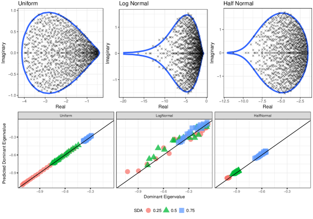
where $P_{X}(x)$ is the species abundance distribution. Figure 4 compares the analytical prediction with the bulk of eigenvalues of $\boldsymbol{M}$ for different distributions of $\boldsymbol{X}$, showing that the solutions of equation 12 closely match the support of the spectrum of $\boldsymbol{M}$.

Figure 4: The top row shows that the analytical predictions for the support of the eigenvalue distribution obtained in equation 12 (solid blue line) correctly predict the support of the spectrum of $\boldsymbol{M}=\boldsymbol{X}\boldsymbol{A}$. In all the three plots, $\boldsymbol{A}$ is built using a bivariate normal distribution with identical marginals $\mu=0$, $\sigma=1/\sqrt{S}$ and correlation $\rho=0$. The diagonal entries of $\boldsymbol{A}$ are fixed at $-2$. We considered three different abundance distributions: uniform ($\boldsymbol{X}$ is sampled from a uniform distribution on [0.25, 1.75]) lognormal ($\boldsymbol{X}$ is sampled from a log-normal distribution with log-mean $0.5$ and log-standard deviation $0.5$) and half-normal ($\bf{X}$ is sampled from a half-normal, shifted rightwards to have support $(1,\infty)$, and with parameter $\theta=1$). The bottom row shows the value of the rightmost eigenvalue of $\bf{M}$ against the analytical prediction for the leading eigenvalue of matrices with the same abundance distributions used above, but varying their variances $\sigma_{X}^{2}$. Different colors correspond to different values of $\sigma$. Each point is an average over $20$ simulations.

Equation 12 also predicts that if $\boldsymbol{A}$ is stable, then $\boldsymbol{M}$ is stable. In fact, equation 12 predicts that the matrix $\boldsymbol{A}$ is stable iff $\mu_{d}+S\sigma^{2}<0$. If this condition is met, it is simple to observe that

$$\frac{Sx^{2}\sigma^{2}}{|\lambda-\mu_{d}x|^{2}}<1$$ (13)

for any complex $\lambda$ with positive real part and any positive real $x$. When this inequality is used in equation 12 one obtains that the points on the boundary of the support, and therefore all the eigenvalues, always have negative real part.

V The stability of large community matrices does not depend on population abundance

In the previous section, we derived the spectrum in the case $\rho=0$, finding that if the interaction matrix $\boldsymbol{A}$ is stable, then $\boldsymbol{M}$ is stable. The goal of this section is to study more deeply the relationship between the stability of $\boldsymbol{A}$ and that of $\boldsymbol{M}$. More specifically, given a stable random matrix $\boldsymbol{A}$, we ask what is the probability of finding a positive diagonal matrix $\boldsymbol{X}$, such that $\boldsymbol{M}=\boldsymbol{X}\boldsymbol{A}$ is stable.

A matrix $\boldsymbol{A}$ is D-stable if, for any positive diagonal matrix $\boldsymbol{X}$, $\boldsymbol{X}\boldsymbol{A}$ is stable Kaszkurewicz2000 . An explicit condition for D-stability that does not require checking all the possible choices of $\boldsymbol{X}$ is not known in dimension larger than four Redheffer1985 . Therefore, it is not known, in general, under which values of $\mu$, $\sigma$, $\rho$ and $\mu_{d}$ random matrices are expected to be D-stable.

A stronger condition for stability is diagonal stability. A matrix $\boldsymbol{A}$ is diagonally stable if there exists a positive diagonal matrix $\boldsymbol{X}$ such that $\boldsymbol{X}\boldsymbol{A}+\boldsymbol{A}^{t}\boldsymbol{X}$ is stable. Interestingly, diagonal stability implies D-stability Kaszkurewicz2000 . As for D-stability, a simple necessary and sufficient test for diagonal stability is not known. On the other hand, it is simple to observe that the stability of $(\boldsymbol{A}+\boldsymbol{A}^{t})/2$ is a sufficient condition for diagonal stability (corresponding to choosing a constant diagonal matrix $\boldsymbol{X}$), and therefore also implies D-stability.

All the eigenvalues of $(\boldsymbol{A}+\boldsymbol{A}^{t})/2$ are real and, if $\boldsymbol{A}$ is a symmetric random matrix of independently distributed entries with bounded higher moments, the bulk of eigenvalues of $(\boldsymbol{A}+\boldsymbol{A}^{t})/2$ follows Wigner’s semicircle distribution Wigner1958 ; Tang2014

$$\varrho_{\frac{\boldsymbol{A}+\boldsymbol{A}^{t}}{2}}(\lambda)=\frac{\sqrt{2S\sigma^{2}(1+\rho)-\left(\lambda-(\mu_{d}-\mu)\right)^{2}}}{\pi S\sigma^{2}(1+\rho)}\ ,$$ (14)

with one outlying eigenvalue equal to $\mu_{d}+(S-1)\mu$.

For positive mean $\mu$, if $\mu>(1+\rho)\sigma/\sqrt{S}$, the rightmost eigenvalue is the outlier. In this case, the rightmost eigenvalue of $\boldsymbol{A}$ and of $(\boldsymbol{A}+\boldsymbol{A}^{t})/2$ are the same. Therefore, for non-negative $\mu$, stable random matrices are almost surely diagonally stable. Since diagonal stability implies D-stability, if $\boldsymbol{A}$ is stable, then $\boldsymbol{M}=\boldsymbol{X}\boldsymbol{A}$ is stable. This argument is in agreement with our formula for the outlier of $\boldsymbol{M}$ in the case of non-vanishing mean $\mu$, obtained in equation 10. For positive mean $\mu$, the rightmost eigenvalue of $\boldsymbol{M}$ is equal to $\mu_{X}\lambda_{\boldsymbol{A}}$, where $\lambda_{\boldsymbol{A}}$ is the rightmost eigenvalue of $\boldsymbol{A}$ and $\mu_{X}$ is positive by definition. The sign of the rightmost eigenvalue of $\boldsymbol{M}$ is therefore the same as that of the rightmost eigenvalue of $\boldsymbol{A}$.

Since a negative $\mu$ only produces a equal shift in the rightmost eigenvalue of $\boldsymbol{A}$, $(\boldsymbol{A}+\boldsymbol{A}^{t})/2$ and $\boldsymbol{M}$, we can restrict our analysis to the case $\mu=0$. For vanishing mean, the rightmost eigenvalue of $(\boldsymbol{A}+\boldsymbol{A}^{t})/2$ is equal to Tang2014

$$\lambda_{\frac{\boldsymbol{A}+\boldsymbol{A}^{t}}{2}}=\mu_{d}+\sqrt{2S\sigma^{2}(1+\rho)}\ ,$$ (15)

which should be compared with the rightmost eigenvalue of $\boldsymbol{A}$

$$\lambda_{\boldsymbol{A}}=\mu_{d}+\sqrt{S\sigma^{2}}(1+\rho)\ .$$ (16)

As shown in Tang2014 ; Grilli2017 , $\lambda_{\frac{\boldsymbol{A}+\boldsymbol{A}^{t}}{2}}\geq\lambda_{\boldsymbol{A}}$ and they are equal in the case $\rho=1$. Equation 15 imposes a sufficient condition on diagonal stability: if

$$\mu_{d}+\sqrt{2S\sigma^{2}(1+\rho)}<0\ ,$$ (17)

$\boldsymbol{A}$ is diagonally stable and, for any choice of positive diagonal matrix $\boldsymbol{X}$, $\boldsymbol{M}=\boldsymbol{X}\boldsymbol{A}$ is stable. The non-trivial regime therefore corresponds to the values of parameters where $\mu_{d}+\sqrt{2S\sigma^{2}(1+\rho)}>0$ and $\mu_{d}+\sqrt{S\sigma^{2}}(1+\rho)<0$ Grilli2017 .

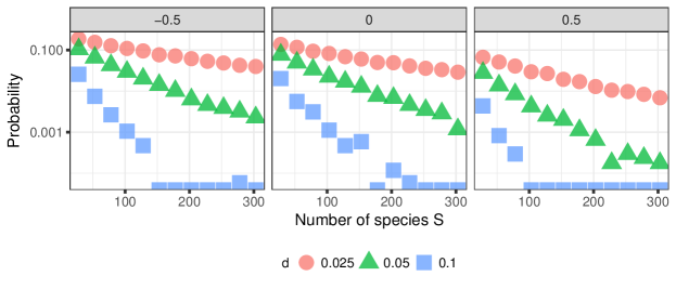
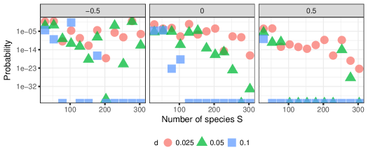
Since an explicit condition for D-stability does not exist, we computed the probability that, given a stable random matrix $\boldsymbol{A}$, a positive diagonal matrix $\boldsymbol{X}$ would make $\boldsymbol{M}=\boldsymbol{X}\boldsymbol{A}$ unstable. Note that, since any matrix has a non-null probability of being generated when entries are sampled from a bivariate distribution with infinite support, this probability is always non-zero. The relevant question in this context is therefore how this probability depends on the number of species $S$. Figure 5 shows that the probability of finding a $\boldsymbol{X}$ with a destabilizing effect decreases exponentially with the number of species $S$, with a rate that depends on the rightmost eigenvalue $\lambda_{\boldsymbol{A}}$ and the correlation $\rho$. This implies that, for large values of $S$, $\boldsymbol{M}$ is almost surely stable if $\boldsymbol{A}$ is stable.

Figure 5: We computed the probability that a matrix $\boldsymbol{M}=\boldsymbol{X}\boldsymbol{A}$ is unstable (i.e., that the leading eigenvalue has positive real part), given that $\boldsymbol{A}$ is a stable random matrix with rightmost eigenvalue equal to $\lambda_{max}=-d$. This probability decreases exponentially with $S$ for different values of $\rho$ ($-0.5$ in the left panel, $0$ in the center and $0.5$ in the right) and $\lambda_{max}$ (different colors). For a given number of species $S$, we construct the random matrix $\boldsymbol{A}$ sampling its entries from a bivariate normal with identical marginals $\mu=0$, $\sigma=1/\sqrt{S}$ and given $\rho$. The diagonal elements of $\boldsymbol{A}$ are all equal and their value is determined in order to have dominant eigenvalue equal to $\lambda_{max}$. The diagonal entries of $\boldsymbol{X}$ were sampled from a uniform distribution on $[0,1]$. For each value of the parameters $\rho$, $\lambda_{max}$ and $S$, we constructed $XXX$ matrices $\boldsymbol{A}$ and $\boldsymbol{X}$ and computed the fraction of matrices $\boldsymbol{M}=\boldsymbol{X}\boldsymbol{A}$ with positive dominant eigenvalue.

VI Fixed points are almost surely stable in large random Lotka-Volterra equations.

If we consider the Lotka-Volterra equations (equation 2), and we set the values of the intrinsic growth rates $\boldsymbol{r}$, the fixed point has components

$$x_{i}^{\ast}=\sum_{j}A^{-1}_{ij}r_{j}\ .$$ (18)

Let us also assume that all these components are positive (i.e., $\boldsymbol{r}$ is inside the feasibility domain). In section V we showed that the matrix obtained by multiplying a stable random matrix $\boldsymbol{A}$ and a random positive diagonal matrix $\boldsymbol{X}$ is more and more likely to be stable as $S$ increases. It is evident (from equation 18) that the components of $\boldsymbol{x}^{\ast}$ are not independent of the entries of the matrix $\boldsymbol{A}$. The presence of this correlation implies that, at least in principle, choosing a random vector $\boldsymbol{r}$ inside the feasibility domain to define $\boldsymbol{X}$ could produce different results from sampling independent entries from a specified species abundance distribution.

In this section we repeat the simulations detailed in section V, but instead of considering a random fixed point $\boldsymbol{x}^{\ast}$, we find the $\boldsymbol{x}^{\ast}$ determined by a random intrinsic growth rate vector $\boldsymbol{r}$ sampled uniformly from the feasibility domain. The most intuitive method for this simulation would consist of taking a random matrix $\boldsymbol{A}$, choosing a value $\boldsymbol{r}$ at random on the unit sphere, checking if it corresponds to a feasible fixed-point using equation 18, and finally computing the eigenvalue of $\boldsymbol{M}=\boldsymbol{X}\boldsymbol{A}$. However, as the number of species $S$ increases this method becomes practically unfeasible. In fact, the fraction of intrinsic growth rate vectors $\boldsymbol{r}$ corresponding to a feasible solution decreases exponentially with $S$ Grilli2017 . If this intuitive method was employed, most of the simulation time would be spent trying to find vectors $\boldsymbol{r}$ inside the feasibility domain.

On the other hand, since the relation between $\boldsymbol{r}$ and $\boldsymbol{x}^{\ast}$ (via equation 18) is bijective, we can easily construct all the vectors $\boldsymbol{r}$ inside the feasibility domain by considering all the possible feasible solution $\boldsymbol{x}^{\ast}$. In section V we specified a distribution on the $\boldsymbol{x}^{\ast}$. This distribution translates to a non-trivial distribution on the $\boldsymbol{r}$ (that can be obtained from equation 18). In this section, we instead assume a distribution on the $\boldsymbol{r}$ and derive a corresponding distribution for the $\boldsymbol{x}^{\ast}$. For instance, if we assume that the vectors $\boldsymbol{r}$ are uniformly distributed on the unit sphere, the distribution of the $\boldsymbol{x}^{\ast}$ reads Grilli2017

$$P(\boldsymbol{x}^{\ast}|\boldsymbol{A})\propto|\det\boldsymbol{A}|\frac{\delta\left(\|\boldsymbol{x}^{\ast}\|^{2}-1\right)}{\|\boldsymbol{A}\boldsymbol{x}^{\ast}\|^{S}}\ .$$ (19)

Sampling vectors $\boldsymbol{x}^{\ast}$ according to this distribution is equivalent to sampling vectors $\boldsymbol{r}$ uniformly from the feasibility domain. It is important to observe that when $\boldsymbol{x}^{\ast}$ is drawn according to this distribution, its entries are not independent and their densities depend on $\boldsymbol{A}$.

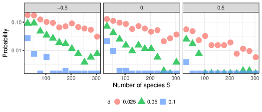
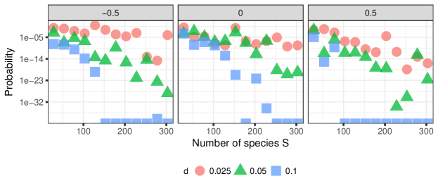
Figure 6 shows the stability of $\boldsymbol{M}=\boldsymbol{X}\boldsymbol{A}$ when the diagonal entries of $\boldsymbol{X}$ are sampled from the probability distribution defined in equation 19. Despite the presence of a correlation between the entries of $\boldsymbol{X}$ and $\boldsymbol{A}$, the result obtained in section V is confirmed: the probability of observing a stable $\boldsymbol{A}$ but an unstable $\boldsymbol{M}$ decreases exponentially with $S$. If the interaction matrix $\boldsymbol{A}$ is stable, in the limit of large $S$, the set of intrinsic growth rates corresponding to feasible unstable solutions has measure zero.

Figure 6: These panels plot the same quantity as of fig 5. Instead of sampling $\boldsymbol{X}$ from a uniform distribution, we used the distribution of eq. 19, which guarantee an unbiased sampling of the intrinsic growth rates of a Lotka-Volterra systems. This sampling method is in fact equivalent to sampling a random interaction matrix $\boldsymbol{A}$ and an intrinsic growth rate vector $\boldsymbol{r}$ inside the feasibility domain and checking the stability of the corresponding feasible fixed point. The exponential decay with increasing $S$ strongly suggests that the set of feasible unstable fixed points has measure zero for large, randomly interacting Lotka-Volterra systems.

VII Discussion

We explored the effect of population abundances on the stability of random interacting ecosystems. We derived an expression for the spectral density of a community matrix that explicitly includes the species abundance distribution. While the effect on the eigenvalues is highly heterogeneous and strongly depends on the specific choice of the abundance distribution, a remarkably simple message emerges for large randomly interacting ecosystems: the community matrix is stable if and only if the interaction matrix is stable. In other words, the abundances of species seem to not affect the sign of the eigenvalues. We further explored this intriguing result by explicitly estimating the probability of choosing a species abundance distribution leading to instability. While for finite systems this probability is always positive, it decreases exponentially with the number of species, confirming what was found studying the spectrum of the community matrix analytically.

Our results strongly suggest that large random matrices are D-stable almost surely: the set of destabilizing positive diagonal matrices has measure zero. This fact has important consequences on Lotka-Volterra systems of equations, implying that feasible unstable fixed-points are very unlikely. This result allows to disentangle the problem of feasibility (how often are fixed points feasible?) from the problem of stability (how often are fixed points stable?), justifying a-posteriori what assumed in many studies on feasibility Rohr2014 ; Grilli2017 and expanding the validity of their results.

The generalized Lotka-Volterra equations display a rich dynamical behavior, leading to limit cycles when two or more species are considered and chaos with three or more species Smale1976 ; Takeuchi1996 . Both limit cycles and chaos require the existence of an unstable fixed point in the interior of the feasibility domain Hofbauer1998 . Since the chance of observing a feasible unstable fixed point decays rapidly when the number of species increases, our results suggest that chaos and limit cycles are extremely rare in large random Lotka-Volterra systems.

A stronger notion than D-stability is diagonal stability. While for Lotka-Volterra systems, the former implies local asymptotic stability of any feasible solution, the latter implies global stability. We showed that large random stable matrices are always D-stable. Under which conditions they are also diagonally stable is an important open problem. A sufficient condition for diagonal stability is negative definiteness Grilli2017 . In the context of random matrices, negative definiteness is equivalent to the condition expressed in equation 17. The condition for negative definiteness should be compared to the condition for stability (see equation 16). For large random matrices, two extreme scenarios are possible: negative definiteness is almost surely a necessary condition for diagonal stability, or stable random matrices are almost surely diagonally stable. It is also possible that the condition for diagonal stability is less trivial, corresponding to values of parameters between the conditions imposed by equations 17 and 16. Even more complicated, it is also possible that a sharp condition for diagonal stability does not exist for random matrices and, in the limit of large $S$, stable and non negative definite random matrices have a non-vanishing probability of being (or not being) diagonally stable.

Our results shed light on one of the most controversial aspects of the classic result of May May1972 and its extensions. Many authors Roberts1974 ; Pimm1979 ; King1983 ; ReviewRMT ; amnatjames ; Jacquet2016 have argued that the unrealistic assumption of constant population abundances was a key choice in May’s paper, suggesting that more realistic abundance distribution would have produced drastically different results. We showed that the conditions obtained in the original paper and in its extension May1972 ; Allesina2012 are in fact valid for any species abundance distribution. In other words, the stability of fixed points (i.e., the stability of the community matrix) is determined only by the stability of the interaction matrix.

Appendix A Notation and goals

We aim to study the spectral density of a matrix $\boldsymbol{M}$ of the form $\boldsymbol{M=XA}$, where $\boldsymbol{X}$ is a positive diagonal matrix and $\boldsymbol{A}$ a random matrix with arbitrary distribution. The diagonal entries of $\boldsymbol{X}$ are drawn from an arbitrary distribution with positive support, mean $\mu_{X}$ and variance $\sigma_{X}^{2}$. The diagonal entries of $\boldsymbol{A}$ are drawn from an arbitrary distribution with negative support, mean $\mu_{d}$ and variance $\sigma_{d}^{2}$. Each pair of off-diagonal entries $(A_{ij},A_{ji})$ is drawn from a bivariate distribution with identical marginal means $\mu$, variances $\sigma^{2}$ and correlation $\rho$.

Let $\boldsymbol{B}$ be an $S\times S$ random matrix with complex eigenvalues $\lambda_{i}$ for $i=1,...,S$. Its spectral density is defined as

$$\varrho(x,y)=\frac{1}{S}\sum_{i=1}^{S}\delta(x-\Re(\lambda_{i}))\delta(y-\Im(\lambda_{i}))$$ (20)

which, in the limit of large $S$, converges to

$$\varrho(x,y)=\mathbb{E}[\delta(x-\Re(\lambda_{i}))\delta(y-\Im(\lambda_{i}))]\ ,$$ (21)

where $\mathbb{E}[\cdot]$ stands for the expectation over matrices in the ensemble.

We introduce the resolvent ³⁷

$$\operatorname*{\mathcal{G}}(\boldsymbol{q};\boldsymbol{B})=\frac{1}{S}\sum_{i=1}^{S}(\lambda_{i}-\boldsymbol{q})^{-1}=\frac{1}{S}\operatorname*{\text{tr}}\left(\boldsymbol{B}-\boldsymbol{q}\boldsymbol{I}\right)^{-1}\ .$$ (22)

The variable $\boldsymbol{q}=\lambda+\epsilon j$ is a quaternion (see section B for definitions and notation) and the resolvent is a function $\operatorname*{\mathcal{G}}:\mathbb{H}\to\mathbb{H}$.

The resolvent and the spectral density are related by the following formulas ³⁷:

$$\operatorname*{\mathcal{G}}(\boldsymbol{q};\boldsymbol{B})=\int dx\ dy\ \varrho(x,y)(x+iy-\boldsymbol{q})^{-1}$$ (23)

and

$$\varrho\left(x,y\right)=-\frac{1}{\pi}\lim_{\epsilon\to 0^{+}}\Re\left(\frac{\partial}{\partial\bar{\lambda}}\operatorname*{\mathcal{G}}(\lambda+\epsilon j;\boldsymbol{B})\right)\biggl{|}_{\lambda=x+iy}\ ,$$ (24)

where $\frac{\partial}{\partial\bar{\lambda}}$ is the Wirtinger derivative

$$\frac{\partial}{\partial\bar{\lambda}}:=\frac{1}{2}\left(\frac{\partial}{\partial x}+i\frac{\partial}{\partial y}\right)\ .$$ (25)

Appendix B Quaternions

When constructing the complex numbers from the real numbers, one defines a variable $i$ to be a root of the equation $x^{2}+1=0$. The algebraic structure of $\mathbb{C}$ descends from the equation $i^{2}=-1$ and the algebraic structure of $\mathbb{R}$. Similarly, the algebra of quaternions $\mathbb{H}$ can be defined by introducing the symbols $i$, $j$ and $k$ and the relations

$$i^{2}=j^{2}=k^{2}=ijk=-1\ .$$ (26)

From these equations all the multiplication rules can be obtained. In particular, it follows that multiplication in $\mathbb{H}$ is not commutative (e.g. $ij=-ji$).

A quaternion $\boldsymbol{q}$ can be written as

$$\textbf{q}=a+bi+cj+dk\ ,$$ (27)

where $a,b,c,d\in\mathbb{R}$. Equivalently, by introducing the two complex numbers $z=a+bi$ and $w=c+di$ and using $k=ij$, one can write

$$\textbf{q}=z+wj\ .$$ (28)

Another equivalent way to represent quaternions is to write them in matrix form

$$\textbf{q}=\left(\begin{matrix}z&w\\ \bar{w}&\bar{z}\\ \end{matrix}\right)\ .$$ (29)

It can be shown that, when written in this form, the multiplication rules of quaternions match the rules of matrix multiplication. In particular, one has that

$$(z+wj)(u+vj)=(zu-w\bar{v})+(zv+w\bar{u})j\ .$$ (30)

We also introduce the operation

$$(z+wj)\circ(u+vj)=zu-wvj\ ,$$ (31)

which, in matrix notation, corresponds to element-by-element multiplication.

The conjugate of a quaternion $\textbf{q}=z+wj$ is defined as $\bar{\boldsymbol{q}}=\bar{z}-wj$. From this definition, one obtains the norm of a quaternion

$$|\boldsymbol{q}|^{2}\equiv\boldsymbol{q}\bar{\boldsymbol{q}}=|z|^{2}+|w|^{2}\ ,$$ (32)

and the inverse

$$\boldsymbol{q}^{-1}\equiv\bar{\boldsymbol{q}}\frac{1}{|\boldsymbol{q}|^{2}}\ .$$ (33)

Moreover, the real part of a quaternion is defined as

$$\Re(\boldsymbol{q})\equiv\bar{\boldsymbol{q}}+\boldsymbol{q}=\Re(z)=a\ .$$ (34)

Appendix C Bulk and outliers of the spectrum of $\boldsymbol{M}$

In this section, we want to show that the mean of $\boldsymbol{A}$ does not affect the bulk of eigenvalues of $\boldsymbol{M}$. We decompose the matrix $\bf{M}$ as

$$\boldsymbol{M}=\boldsymbol{X}(\boldsymbol{D}-\mu\boldsymbol{I}+\boldsymbol{B}+\mu\boldsymbol{1})$$ (35)

where $\boldsymbol{I}$ is the identity matrix, $\boldsymbol{1}$ is a matrix of ones and $\boldsymbol{D}$ is the diagonal matrix consisting of the diagonal entries of $\boldsymbol{A}$. Written in this way, $\boldsymbol{B}$ is a random matrix with mean zero and null diagonal. We will show that the bulk of the spectrum of $\boldsymbol{M}$ is equivalent to the bulk of eigenvalues of the matrix $\boldsymbol{J}=\boldsymbol{X}(\boldsymbol{D}-\mu\boldsymbol{I}+\boldsymbol{B})$.

Using equation 35, the resolvent of $\boldsymbol{M}$ can be written

$$\operatorname*{\mathcal{G}}(\boldsymbol{q};\boldsymbol{M})=\mathbb{E}[\frac{1}{S}\operatorname*{\text{tr}}\left(\boldsymbol{q}\boldsymbol{I}-\boldsymbol{X}\boldsymbol{D}-\mu\boldsymbol{X}-\boldsymbol{X}\boldsymbol{B}-\mu\boldsymbol{X}\boldsymbol{1}\right)^{-1}]=\mathbb{E}[\frac{1}{S}\operatorname*{\text{tr}}\left(\boldsymbol{q}\boldsymbol{I}-\boldsymbol{J}-\mu\boldsymbol{X}\boldsymbol{1}\right)^{-1}].$$ (36)

Using the Sherman-Morrison formula, if $\boldsymbol{Y}$ and $\boldsymbol{Y+Z}$ are invertible matrices and $\boldsymbol{Z}$ has rank 1, then

$$(\boldsymbol{Y}+\boldsymbol{Z})^{-1}=\boldsymbol{Y}^{-1}+\frac{1}{1+\operatorname*{\text{tr}}(\boldsymbol{Z}\boldsymbol{Y}^{-1})}\boldsymbol{Y}^{-1}\boldsymbol{Z}\boldsymbol{Y}^{-1}\ .$$ (37)

Since $\mu\boldsymbol{X}\boldsymbol{1}$ has rank one, we have

$$\left(\boldsymbol{q}\boldsymbol{I}-\boldsymbol{J}-\mu\boldsymbol{X}\boldsymbol{1}\right)^{-1}=(\textbf{q}\boldsymbol{I}-\boldsymbol{J})^{-1}+\frac{1}{1+\operatorname*{\text{tr}}(\mu\boldsymbol{X}\boldsymbol{1}(\textbf{q}\boldsymbol{I}-\boldsymbol{J})^{-1})}(\textbf{q}\boldsymbol{I}-\boldsymbol{J})^{-1}\mu\boldsymbol{X}\boldsymbol{1}(\textbf{q}\boldsymbol{I}-\boldsymbol{J})^{-1}\ .$$ (38)

By introducing the linear operator $\langle\cdot\rangle$ defined by $\langle\boldsymbol{C}\rangle=\frac{1}{S}\operatorname*{\text{tr}}{\boldsymbol{C}}$ for an $S\times S$ matrix $\boldsymbol{C}$, we obtain

$$\operatorname*{\mathcal{G}}(\boldsymbol{q};\boldsymbol{M})=\operatorname*{\mathcal{G}}(\boldsymbol{q};\boldsymbol{J})+\frac{\mu}{1+S\mu\langle\boldsymbol{X}\boldsymbol{1}(\textbf{q}\boldsymbol{I}-\boldsymbol{J})^{-1})\rangle}\langle(\textbf{q}\boldsymbol{I}-\boldsymbol{J})^{-1}\boldsymbol{X}\boldsymbol{1}(\textbf{q}\boldsymbol{I}-\boldsymbol{J})^{-1}\rangle\ .$$ (39)

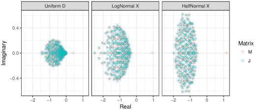
In the limit of large $S$, the contribution from the second term in 39 is subleading. Therefore, the resolvent of $\boldsymbol{M}$ converges to the resolvent of $\boldsymbol{J}$ when $S$ is large. In other words, as shown in Figure A1, the bulks of the eigenvalues of $\boldsymbol{M}$ and $\boldsymbol{J}$ are the same — up to finite-size corrections.

Figure A1: The eigenvalue distributions for $\boldsymbol{M}$ and $\boldsymbol{J}$ of size $S=250$ with $\boldsymbol{D}$ and $\boldsymbol{X}$ following different distributions. In each case, $\boldsymbol{A}$ is a bivariate normal distribution with identical marginals $\mu=2/S$, $\sigma=0.5$ and $\rho=0$. Uniform D has $\boldsymbol{D}$ following a uniform distribution on $(-1.5,-0.5)$. LogNormal X has $\boldsymbol{X}$ following a log-normal distribution with log-mean $0$ and log-standard deviation $0.35$. HalfNormal X has $\boldsymbol{X}$ following a half-normal distribution with support $(1,\infty)$ and parameter $\theta=1$.

Appendix D The case $\sigma=0$

When $\sigma=0$, we derive the spectrum of a matrix $\boldsymbol{Q}=\boldsymbol{X}\left(\boldsymbol{D}+\mu\boldsymbol{1}\right)$. This case corresponds to setting $\boldsymbol{B}=0$ in equation 35. As shown in the main text, the spectral density of the matrix $\boldsymbol{Q}$ is characterized by the presence of an outlier. In this section, we focus on the bulk of eigenvalues.

If we take $\boldsymbol{J}=\boldsymbol{X}(\boldsymbol{D}-\mu\boldsymbol{I}+\boldsymbol{B})$ as before and set $\sigma=0$, then $\boldsymbol{B}=0$, so that $\boldsymbol{M}=\boldsymbol{Q}$ and $\boldsymbol{J}=\boldsymbol{X}(\boldsymbol{D}-\mu\boldsymbol{I})$. The bulk of eigenvalues of $\boldsymbol{Q}$ and $\boldsymbol{J}$ will be the same. The resolvent of $\boldsymbol{J}$ in the case $\sigma=0$ reads

$$G(\textbf{q};\boldsymbol{J}) =\frac{1}{S}\operatorname*{\text{tr}}\left(\textbf{q}-\boldsymbol{J}\right)^{-1}$$ (40)

$$=\frac{1}{S}\operatorname*{\text{tr}}\left(\textbf{q}-\boldsymbol{X}\boldsymbol{D}\right)^{-1}$$

$$=\frac{1}{S}\sum_{i=1}^{S}\frac{1}{q-X_{i}D_{i}}$$

since $\textbf{q}-\boldsymbol{X}(\boldsymbol{D}-\mu\boldsymbol{I})$ is symmetric. In the limit of large $S$, the sum in eq. LABEL:resolventQ tends toward $\mathbb{E}\left[(\textbf{q}-\boldsymbol{X}\boldsymbol{D})^{-1}\right]$. If $P_{XD}(x,s)$ is the joint distribution of the entries of $\boldsymbol{X}$ and $\boldsymbol{D}$, we obtain

$$G(\textbf{q};\boldsymbol{J}) =\frac{1}{S}\sum_{i=1}^{S}\frac{1}{q-X_{i}D_{i}+\mu X_{i}}$$ (41)

$$=\mathbb{E}\left[(\textbf{q}-\boldsymbol{X}(\boldsymbol{D}-\mu\boldsymbol{I}))^{-1}\right]$$

$$=\int dx\ ds\ \frac{P_{XD}(x,s)}{q-xs}\ .$$

In the case of a constant diagonal matrix $\boldsymbol{D}=d\boldsymbol{I}$, this equation simplifies to

$$G(\textbf{q};\boldsymbol{J})=\int dx\ \frac{P_{X}(x)}{q-xd}=\frac{1}{d}\int dy\ \frac{P_{X}\left(\frac{y}{d}\right)}{q-y}\\$$ (42)

with the change of variables $y=xd$. Using equation 23, we obtain that the spectral density $\varrho_{\boldsymbol{J}}(\lambda)$ will be

$$\varrho_{\boldsymbol{J}}(\lambda)=\frac{1}{d}P_{X}\left(\frac{\lambda}{d}\right)\ .$$ (43)

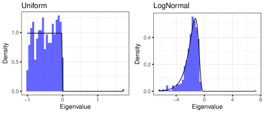
In Figure A2, we plot the prediction from Equation 43 against the bulk of the spectrum of $\boldsymbol{Q}$ for two distributions of $\boldsymbol{X}$.

Figure A2: Histograms of the eigenvalue distribution for two matrices $\boldsymbol{Q}$ of size $S=1500$. In each matrix, $\sigma_{d}=0$, $\mu_{d}=-1$ and $\mu=5/S$. The Uniform plot has $\boldsymbol{X}$ following a uniform distribution on $(0,1)$ and the LogNormal plot has $\boldsymbol{X}$ following a log-normal distribution with log-mean and log-standard deviation both $0.5$.

Appendix E Derivation of the spectral density using the cavity method

In section C, we showed that we can isolate the effect of $\mu\neq 0$. In this section, we use the cavity method  ^{26, 27} to derive the spectrum of the matrix $\boldsymbol{J}=\boldsymbol{X}(\boldsymbol{D}-\mu\boldsymbol{I}+\boldsymbol{B})$, where $\boldsymbol{D}$ and $\boldsymbol{X}$ are two random diagonal matrices and $\boldsymbol{B}$ is a random matrix following the elliptic law.

We introduce the resolvent matrix

$$\boldsymbol{G}=(\boldsymbol{M}-\boldsymbol{q}\boldsymbol{I})^{-1}\ ,$$ (44)

The resolvent can be written as

$$\operatorname*{\mathcal{G}}(\boldsymbol{q};\boldsymbol{B})=\frac{1}{S}\operatorname*{\text{tr}}\boldsymbol{G}\ .$$ (45)

Note that each element of the resolvent matrix is a quaternion. In particular we will use the notation

$$\boldsymbol{G}_{ik}=\alpha_{ik}+\beta_{ik}j\equiv\left(\begin{matrix}\alpha_{ik}&\beta_{ik}\\ \bar{\beta_{ik}}&\bar{\alpha_{ik}}\\ \end{matrix}\right)\ ,$$ (46)

while $\operatorname*{\mathcal{G}}=\alpha+\beta j$, where $\alpha=\sum_{i}\alpha_{ii}/S$ and $\beta=\sum_{i}\beta_{ii}/S$. The cavity method allows us to compute the elements of $\boldsymbol{G}$ (and therefore the resolvent $\operatorname*{\mathcal{G}}$) if the matrix $\boldsymbol{M}$ has a tree structure ^{26, 27}. It also allows to compute the spectral density for large, densely connected, random matrices ^{26, 27, 7}. In the limit of large $S$, for a densely connected matrix $\boldsymbol{M}$, the cavity equations read ^{27, 7}

$$\boldsymbol{G}_{il}\equiv\left(\begin{matrix}\alpha_{il}&\beta_{il}\\ \bar{\beta}_{il}&\bar{\alpha}_{il}\\ \end{matrix}\right)=-\left(\left(\begin{matrix}\lambda&\epsilon\\ \epsilon&\bar{\lambda}\\ \end{matrix}\right)+\sum_{jk}\left(\begin{matrix}M_{ij}&0\\ 0&M_{ji}\\ \end{matrix}\right)\left(\begin{matrix}\alpha_{jk}&\beta_{jk}\\ \bar{\beta}_{jk}&\bar{\alpha}_{jk}\\ \end{matrix}\right)\left(\begin{matrix}M_{kl}&0\\ 0&M_{lk}\\ \end{matrix}\right)\right)^{-1}\ .$$ (47)

By introducing

$$\tilde{\boldsymbol{M}}_{ij}=\left(\begin{matrix}M_{ij}&0\\ 0&M_{ji}\\ \end{matrix}\right)\ ,$$ (48)

we obtain the more compact equation

$$\boldsymbol{G}_{il}=-\left(\boldsymbol{q}+\sum_{jk}\tilde{\boldsymbol{M}}_{ij}\boldsymbol{G}_{jk}\tilde{\boldsymbol{M}}_{kl}\right)^{-1}\ .$$ (49)

Our goal is to find the resolvent for a random matrix of the form $\boldsymbol{M}=\boldsymbol{X}(\boldsymbol{D}+\boldsymbol{B})$, where $\boldsymbol{X}$ and $\boldsymbol{D}$ are diagonal matrices, while $\boldsymbol{B}$ is a random matrix following the elliptic law. We introduce the matrix

$$\left(\begin{matrix}-\boldsymbol{q}\boldsymbol{I}&\tilde{\boldsymbol{X}}\\ -\tilde{\boldsymbol{D}}-\tilde{\boldsymbol{B}}&\boldsymbol{I}\end{matrix}\right)\ ,$$ (50)

which, when quaternions are represented as $2\times 2$ matrices, is a $4S\times 4S$ matrix. In particular, this matrix is composed of $S^{2}$ $4\times 4$ blocks with entries

$$\left(\begin{matrix}-\lambda\delta_{ij}&-\epsilon\delta_{ij}&X_{ii}\delta_{ij}&0\\ -\epsilon\delta_{ij}&-\bar{\lambda}\delta_{ij}&0&X_{ii}\delta_{ij}\\ -D_{ii}\delta_{ij}-B_{ij}&0&\delta_{ij}&0\\ 0&-D_{ii}\delta_{ij}-B_{ji}&0&\delta_{ij}\end{matrix}\right)\ .$$ (51)

It is simple to observe that

$$\boldsymbol{T}=\left(\begin{matrix}-\bf{q}&\boldsymbol{X}\\ \boldsymbol{-A}&\boldsymbol{I}\end{matrix}\right)^{-1}=\left(\begin{matrix}\left(-\boldsymbol{q}\boldsymbol{I}+\boldsymbol{X}(\boldsymbol{D}+\boldsymbol{B})\right)^{-1}&...\\ ...&...\end{matrix}\right)=\left(\begin{matrix}\boldsymbol{G}&...\\ ...&...\end{matrix}\right)\ .$$ (52)

If we write the cavity equation for $\boldsymbol{T}$, assuming dense matrices, we obtain

$$\boldsymbol{T}_{ii}=\left[\left(\begin{matrix}-\boldsymbol{q}&\tilde{\boldsymbol{X}}_{ii}\\ -\tilde{\boldsymbol{D}}_{ii}&1\end{matrix}\right)-\sum_{j,k}\left(\begin{matrix}\boldsymbol{0}&\boldsymbol{0}\\ \tilde{\boldsymbol{B}}_{ij}&\boldsymbol{0}\end{matrix}\right)\boldsymbol{T}_{jk}\left(\begin{matrix}\boldsymbol{0}&\boldsymbol{0}\\ \tilde{\boldsymbol{B}}_{ki}&\boldsymbol{0}\end{matrix}\right)\right]^{-1}\ .$$ (53)

We can apply the law of large numbers to take the expectation of the matrices over $\boldsymbol{B}$. Using the following expectations over the elements of $\boldsymbol{B}$

$$\begin{split}\mathbb{E}\left[B_{ij}\right]&=0\\ \mathbb{E}\left[(B_{ij})^{2}\right]&=\frac{\tilde{\sigma}^{2}}{S}\\ \mathbb{E}\left[B_{ij}B_{ji}\right]&=\rho\frac{\tilde{\sigma}^{2}}{S}\ ,\end{split}$$ (54)

we find that the non-diagonal terms of $\boldsymbol{T}$ go to zero in expectation. By introducing the notation

$$\boldsymbol{T}_{ii}\equiv\left(\begin{array}[]{cc}\boldsymbol{G}_{ii}&\boldsymbol{T}^{b}_{ii}\\ ...&...\end{array}\right)$$ (55)

and

$$\boldsymbol{T}_{\star}\equiv\frac{1}{S}\sum_{i}\boldsymbol{T}_{ii}=\left(\begin{array}[]{cc}\operatorname*{\mathcal{G}}&\boldsymbol{T}^{b}_{\star}\\ ...&...\end{array}\right)\ ,$$ (56)

the cavity equations for the diagonal terms read

$$\boldsymbol{T}_{ii}=\left(\begin{array}[]{cc}-\boldsymbol{q}&X_{ii}\\ -D_{ii}-\boldsymbol{t}\circ\boldsymbol{T}^{b}_{\star}&\boldsymbol{I}\end{array}\right)^{-1}$$ (57)

where $\boldsymbol{T}_{\star}=\sum_{i}\boldsymbol{T}_{ii}/S$, while $\bf{t}=\tilde{\sigma}^{2}\rho+\tilde{\sigma}^{2}j$ with $\circ$ denoting the element-by-element matrix product (see section B).

We obtain a system of $2S$ quaternionic equations

$$\begin{cases}\displaystyle\boldsymbol{T}^{b}_{ii}=-X_{ii}\left(-\boldsymbol{q}-X_{ii}\left(-D_{ii}-\boldsymbol{t}\circ\boldsymbol{T}^{b}_{\star}\right)\right)^{-1}\\ \displaystyle\boldsymbol{G}_{ii}=\left(-\boldsymbol{q}-X_{ii}\left(-D_{ii}-\boldsymbol{t}\circ\boldsymbol{T}^{b}_{\star}\right)\right)^{-1}\ ,\end{cases}$$ (58)

where

$$\boldsymbol{T}^{b}_{\star}=\frac{1}{S}\sum_{i}\boldsymbol{T}_{ii}\ .$$ (59)

Assuming that the elements of $\boldsymbol{X}$ and $\boldsymbol{D}$ are drawn from a given joint distirbution $P_{XD}$, we obtain the following two equations

$$\begin{cases}\displaystyle\boldsymbol{T}^{b}_{\star}=-\int dx\ ds\ P_{XD}(x,s)x\left(-\boldsymbol{q}+x(s+\boldsymbol{t}\circ\boldsymbol{T}^{b}_{\star})\right)^{-1}\\ \displaystyle\operatorname*{\mathcal{G}}=\int dx\ ds\ P_{XD}(x,s)\left(-\boldsymbol{q}+x(s+\boldsymbol{t}\circ\boldsymbol{T}^{b}_{\star})\right)^{-1}\ .\end{cases}$$ (60)

At this point one can use $\boldsymbol{T}^{b}_{\star}=\alpha^{b}+\beta^{b}j$ and $\operatorname*{\mathcal{G}}=\alpha+\beta j$ to obtain $4$ equations of complex variables. It is simple to observe that $\beta^{b}=0$ is always a solution and $\beta=0$ if and only if $\beta^{b}=0$. The solution $\beta=\beta^{b}=0$ always corresponds to a null specral density ³⁷. The values of $\lambda$ for which a non-zero solution for $\beta$ exist correspond to the support of the spectral density. Setting $\beta^{b}\neq 0$ and $\epsilon=0$, one obtains from equation 60

$$\begin{cases}\displaystyle\alpha^{b}=\int dx\ ds\ P_{XD}(x,s)\frac{x\left(\bar{\lambda}-sx-x\tilde{\sigma}^{2}\rho\bar{\alpha}^{b}\right)}{|\lambda+x\left(-s-\alpha^{b}\rho\tilde{\sigma}^{2}\right)|^{2}+|x\tilde{\sigma}^{2}\beta^{b}|^{2}}\\ \displaystyle 1=\int dx\ ds\ P_{XD}(x,s)\frac{x^{2}\tilde{\sigma}^{2}}{|\lambda+x\left(-s-\alpha^{b}\rho\tilde{\sigma}^{2}\right)|^{2}+|x\tilde{\sigma}^{2}\beta^{b}|^{2}}\ .\end{cases}$$ (61)

By using the second equation, the system of equations further simplifies to

$$\begin{cases}\displaystyle\alpha^{b}+\rho\bar{\alpha}^{b}=\int dx\ ds\ P_{XD}(x,s)\frac{x\left(\bar{\lambda}-sx\right)}{|\lambda+x\left(-s-\alpha^{b}\rho\tilde{\sigma}^{2}\right)|^{2}+|x\tilde{\sigma}^{2}\beta^{b}|^{2}}\\ \displaystyle 1=\int dx\ ds\ P_{XD}(x,s)\frac{x^{2}\tilde{\sigma}^{2}}{|\lambda+x\left(-s-\alpha^{b}\rho\tilde{\sigma}^{2}\right)|^{2}+|x\tilde{\sigma}^{2}\beta^{b}|^{2}}\ .\end{cases}$$ (62)

The values of $\lambda$ for which a solution of equations 62 exists are contained in the support of the spectral density. We assume that the solution $\beta^{b}$ of these equations vanishes at the boundaries of the support. In this case, the points at the boundaries of the support of the spectral density are the complex solutions $\lambda$ of

$$\begin{cases}\displaystyle\alpha^{b}+\rho\bar{\alpha}^{b}=\int dx\ ds\ P_{XD}(x,s)\frac{x\left(\bar{\lambda}-sx\right)}{|\lambda+x\left(-s-\alpha^{b}\rho\tilde{\sigma}^{2}\right)|^{2}}\\ \displaystyle 1=\int dx\ ds\ P_{XD}(x,s)\frac{x^{2}\tilde{\sigma}^{2}}{|\lambda+x\left(-s-\alpha^{b}\rho\tilde{\sigma}^{2}\right)|^{2}}\ ,\end{cases}$$ (63)

where we used the second equation

We should note here that this method does not prove the convergence in any mode of the spectral bulk, but does yield a prediction for its support.

Support of the spectral density in the case $\rho=0$

In the case $\rho=0$, the two equations 63 become independent, and the support is defined by the solutions of

$$1=\tilde{\sigma}^{2}\int dx\ ds\ P_{XD}(x,s)\frac{x^{2}}{|\lambda-sx|^{2}}\ .$$ (64)

In the case $\tilde{\sigma}_{d}^{2}=0$, this equation further simplifies to

$$1=\tilde{\sigma}^{2}\int dx\ P_{X}(x)\frac{x^{2}}{|\lambda-\mu_{d}x|^{2}}\ .$$ (65)

For instance, if $P_{X}$ is a uniform distribution on $[0,1]$, one can evaluate the integral, obtaining

$$1 =\int_{0}^{1}dx\ \frac{x^{2}\tilde{\sigma}^{2}}{|\lambda-\mu_{d}x|^{2}}$$ (66)

$$=\frac{\tilde{\sigma}^{2}}{\mu_{d}^{3}}\left(2\lambda\mu_{d}-\mu_{d}^{2}+2\lambda(\mu_{d}-\lambda)\log\left|\frac{\lambda}{\lambda-\mu_{d}}\right|\right)\ .$$

The complex solutions $\lambda$ of this equation define the boundary of the support of the spectral density.

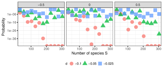
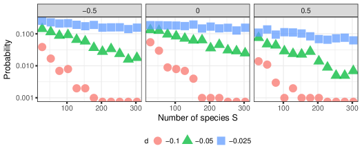
Figure A3: The conditional probability of a matrix $\boldsymbol{M}$ becoming stable given an unstable interaction matrix $\boldsymbol{A}$ with leading eigenvalue $-d$. The off-diagonal elements of $\boldsymbol{A}$ follow a bivariate normal distribution and, for each $S$, $\mu$ =0, $\sigma=1/\sqrt{S}$ and $\rho=-0.5$, $0$ or $0.5$. The elements of $\boldsymbol{X}$ are drawn from a uniform distribution on $(0,1)$, so that $\mu_{X}=0.5$ and $\sigma_{X}^{2}=\frac{1}{12}$. The diagonal elements of $\boldsymbol{A}$ are fixed at $-1$ since $\sigma_{d}^{2}=0$ and $\mu_{D}=-1$. Each probability is calculated from $1000$ trials from $1000$ simulated matrices $\boldsymbol{M}=\boldsymbol{XA}$.

Figure A4: As in Figure A3, except now the conditional probability is weighted by feasibility.

Figure A5: The conditional probability of a matrix $\boldsymbol{M}$ becoming unstable given a stable interaction matrix $\boldsymbol{A}$ with leading eigenvalue $-d$. The off-diagonal elements of $\boldsymbol{A}$ follow a bivariate normal distribution and, for each $S$, $\mu$ =0, $\sigma=1/\sqrt{S}$ and $\rho=-0.5$, $0$ or $0.5$. The elements of $\boldsymbol{X}$ are drawn from a uniform distribution on $(0,1)$, so that $\mu_{X}=0.5$ and $\sigma_{X}^{2}=\frac{1}{12}$. The diagonal elements of $\boldsymbol{A}$ follow a uniform distribution on $(-0.75,-1.25)$ so that $\sigma_{d}^{2}=\frac{1}{48}$ and $\mu_{D}=-1$. Each probability is calculated from $1000$ trials from $1000$ simulated matrices $\boldsymbol{M}=\boldsymbol{XA}$.

Figure A6: As in Figure A5, except now the conditional probability is weighted by feasibility.

References

• 1 May, R. M. How Many Species Are There on Earth? Science 241(4872) (1988).
• 2 Arditi, R. and Ginzburg, L. R. How Species Interact: Altering the Standard View on Trophic Ecology. Oxford University Press, (2012).
• 3 May, R. M. Will a Large Complex System be Stable? Nature 238(5364), 413–414, aug (1972).
• 4 Allesina, S. and Tang, S. Stability criteria for complex ecosystems. Nature 483(7388), 205–208, feb (2012).
• 5 Allesina, S. and Tang, S. The stability–complexity relationship at age 40: a random matrix perspective. Population Ecology 57(1), 63–75, jan (2015).
• 6 Allesina, S., Grilli, J., Barabás, G., Tang, S., Aljadeff, J., and Maritan, A. Predicting the stability of large structured food webs. Nature communications 6, 7842, jan (2015).
• 7 Grilli, J., Rogers, T., and Allesina, S. Modularity and stability in ecological communities. Nature Communications 7 (2016).
• 8 Bell, G. Neutral Macroecology. Science 293(5539) (2001).
• 9 Fisher, R., Corbet, A. S., and Williams, C. B. The Relation Between the Number of Species and the Number of Individuals in a Random Sample of an Animal Population. The Journal of Animal Ecology 12(1), 42, may (1943).
• 10 Preston, F. W. The Commonness, and Rarity, of Species. Ecology 29(3), 254–283 (1948).
• 11 Volkov, I., Banavar, J. R., Hubbell, S. P., and Maritan, A. Patterns of relative species abundance in rainforests and coral reefs. Nature 450(7166), 45–9, nov (2007).
• 12 Caswell, H. Community Structure: A Neutral Model Analysis. Ecological Monographs 46(3), 327–354, feb (1976).
• 13 Hubbell, S. P. The Unified Neutral Theory of Biodiversity and Biogeography. Princeton University Press, (2001).
• 14 Volkov, I., Banavar, J. R., Hubbell, S. P., and Maritan, A. Neutral theory and relative species abundance in ecology. Nature 424(6952), 1035–7, aug (2003).
• 15 Azaele, S., Suweis, S., Grilli, J., Volkov, I., Banavar, J. R., and Maritan, A. Statistical mechanics of ecological systems: Neutral theory and beyond. Reviews of Modern Physics 88(3), 035003, jul (2016).
• 16 MacArthur, R. H. On The Relative Abundance of Bird Species. Proceedings of the National Academy of Sciences 43(3), 293–295, mar (1957).
• 17 Vandermeer, J. H. and MacArthur, R. H. A Reformulation of Alternative (b) of the Broken Stick Model of Species Abundance. Ecology 47(1), 139–140 (1966).
• 18 James, A., Plank, M. J., Rossberg, A. G., Beecham, J., Emmerson, M., and Pitchford, J. W. Constructing Random Matrices to Represent Real Ecosystems. The American Naturalist 185(5), 680–692, may (2015).
• 19 Jacquet, C., Moritz, C., Morissette, L., Legagneux, P., Massol, F., Archambault, P., and Gravel, D. No complexity–stability relationship in empirical ecosystems. Nature Communications 7, 12573, aug (2016).
• 20 Roberts, A. The stability of a feasible random ecosystem. Nature 251(5476), 607–608, oct (1974).
• 21 Rohr, R. P., Saavedra, S., and Bascompte, J. On the structural stability of mutualistic systems. Science 345(6195), 1253497–1253497, jul (2014).
• 22 Stone, L. The Google matrix controls the stability of structured ecological and biological networks. Nature Communications 7, 12857, sep (2016).
• 23 Grilli, J., Adorisio, M., Suweis, S., Barabás, G., Banavar, J. R., Allesina, S., and Maritan, A. Feasibility and coexistence of large ecological communities. Nature Communications 8, 0, feb (2017).
• 24 Nguyen, H. and O’Rourke, S. The elliptic law. arXiv preprint 1 (2012).
• 25 O’Rourke, S. and Renfrew, D. Low rank perturbations of large elliptic random matrices. Electronic Journal of Probability 19 (2014).
• 26 Rogers, T., Castillo, I. P., Kühn, R., and Takeda, K. Cavity approach to the spectral density of sparse symmetric random matrices. Physical Review E 78(3), 031116, sep (2008).
• 27 Rogers, T. and Castillo, I. P. Cavity approach to the spectral density of non-Hermitian sparse matrices. Physical Review E 79(1), 012101, jan (2009).
• 28 Kaszkurewicz, E. and Bhaya, A. Matrix Diagonal Stability in Systems and Computation. Birkhäuser Boston, Boston, MA, (2000).
• 29 Redheffer, R. Volterra Multipliers II. SIAM Journal on Algebraic Discrete Methods 6(4), 612–623, oct (1985).
• 30 Wigner, E. P. On the Distribution of the Roots of Certain Symmetric Matrices. The Annals of Mathematics 67(2), 325, mar (1958).
• 31 Tang, S. and Allesina, S. Reactivity and stability of large ecosystems. Frontiers in Ecology and Evolution 2, 21, jun (2014).
• 32 Smale, S. On the differential equations of species in competition. Journal of Mathematical Biology 3(1), 5–7 (1976).
• 33 Takeuchi, Y. Global dynamical properties of Lotka-Volterra systems. World Scientific, (1996).
• 34 Hofbauer, J. and Sigmund, K. Evolutionary Games and Population Dynamics. (1998).
• 35 Pimm, S. L. Complexity and Stability: Another Look at MacArthur’s Original Hypothesis. Oikos 33(3), 351 (1979).
• 36 King, A. W. and Pimm, S. L. Complexity, Diversity, and Stability: A Reconciliation of Theoretical and Empirical Results. The American Naturalist 122(2), 229–239, aug (1983).
• 37 Rogers, T. Universal sum and product rules for random matrices. Journal of Mathematical Physics 51(9), 093304, sep (2010).