IFUP-TH-2017
Large-$N$ ${\mathbb{C}P}^{N-1}$ sigma model on a finite interval and the renormalized string energy

Abstract

We continue the analysis started in a recent paper of the large-$N$ two-dimensional ${\mathbb{C}P}^{N-1}$ sigma model, defined on a finite space interval $L$ with Dirichlet (or Neumann) boundary conditions. Here we focus our attention on the problem of the renormalized energy density ${\cal E}(x,\Lambda,L)$ which is found to be a sum of two terms, a constant term coming from the sum over modes, and a term proportional to the mass gap. The approach to ${\cal E}(x,\Lambda,L)\to\tfrac{N}{4\pi}\Lambda^{2}$ at large $L\Lambda$ is shown, both analytically and numerically, to be exponential: no power corrections are present and in particular no Lüscher term appears. This is consistent with the earlier result which states that the system has a unique massive phase, which interpolates smoothly between the classical weakly-coupled limit for $L\Lambda\to 0$ and the “confined” phase of the standard ${\mathbb{C}P}^{N-1}$ model in two dimensions for $L\Lambda\to\infty$.

1 Introduction

Recently we embarked on the investigation of the bosonic ${\mathbb{C}P}^{N-1}$ model [1, 2], defined on finite space interval $L$, i.e., on a finite width worldstrip, in the large $N$ approximation [3]. Such a system could provide a useful model for various physical situations. For instance, it appears as the low-energy effective theory describing the quantum excitations of the monopole-vortex soliton complex [4, 5, 6, 7] in hierarchically broken gauge symmetries, such as $SU(N+1)\to SU(N)\times U(1)\to{\bf 1}$ in a color-flavor locked $SU(N)$ symmetric vacuum. The ${\mathbb{C}P}^{N-1}$ model describes the nonAbelian orientational zeromodes of the nonAbelian vortex (string) [8, 9, 10], whereas its boundaries represent the monopoles arising from a higher-scale gauge-symmetry breaking, carrying the same orientational ${\mathbb{C}P}^{N-1}$ moduli. NonAbelian monopoles, not plagued by the well-known difficulties, could emerge in such a context. The fate of the nonAbelian monopoles as a quantum mechanical entity is then linked to the phase of the low-energy ${\mathbb{C}P}^{N-1}$ effective action attached to it.

In [3] it was found that the quantum saddle-point equations describing the ${\mathbb{C}P}^{N-1}$ model with Dirichlet or Neumann boundary conditions has a unique solution under certain conditions. In the large-$L$ limit, this solution approaches smoothly the well-known confining phase of the standard 2D ${\mathbb{C}P}^{N-1}$ system. A phase transition between a Higgs-like phase and the confining phase for a shorter $L$, which was claimed to be present in the literature [11], was shown not to exist in the system.

The model is interesting also from a formal point of view, as it provides a prototype model of a quantum system of varying dimensions in the presence of dynamical mass generation: it interpolates between a 2D QFT (in the $L\to\infty$ limit) with all well-known phenomena such as asymptotic freedom and confinement and a 1D system in the $L\to 0$ limit - quantum mechanics. For shorter strings of length $L\leq 1/\Lambda$, quantum fluctuations of the ${\mathbb{C}P}^{N-1}$ fields $n_{i}$, ($i=1,2,\ldots,N$) remain weakly coupled, as they lack sufficient 2D spacetime “volume” in which the fields fluctuate. With the Dirichlet condition, the system reduces effectively to a classical system in the $L\ll 1/\Lambda$ limit.

In this paper, we delve in more detail into the properties of the large-$N$ ${\mathbb{C}P}^{N-1}$ model on a finite-width worldsheet. First, with a more refined numerical method we improve the precision of the solution to the generalized gap equation. This enables us to explore a larger region of the parameter space and in particular the limit of large $L$. The second problem is to understand the energy density of the string itself as a function of $x$, computed at the functional saddle point, completing the analysis presented in [3]. The third problem is to clarify the approach to the QFT ($L\to\infty$) limit of our system; this involves the question of certain consistency with the known field-theory limit, as well as of figuring out interesting $L$-dependent effects. It will be seen that power-behaved corrections such as the Lüscher term are absent. This is consistent as all fields acquire dynamically generated mass; at the same time no spontaneous breakdown of the global $SU(N)$ symmetry takes place.

The paper is organized as follows. In Section 2 we review the ${\mathbb{C}P}^{N-1}$ model on a finite strip and also present new numerically improved results which allows to reach higher values of $L$ than before. In Section 3 the generalized gap equation is re-derived, paying special attention to the anomalous term that arises in the functional variation, which is analogous to the axial anomaly. In Section 4 we consider the energy density in detail, its various contributions, and its $L\to\infty$ limit. In Section 5 we study an analytical Ansatz that describes the large but finite $L\gg 1/\Lambda$ and the approach to the $L\to\infty$ limit. The numerical results for the renormalized energy density are presented in Section 6. In Section 7 we discuss the Casimir force. Our conclusion is in Section 8. Some details of our analysis are given in Appendices A $\sim$ F.

2 Review of the ${\mathbb{C}P}^{N-1}$ model on a finite width worldsheet

The classical action for the ${\mathbb{C}P}^{N-1}$ sigma model is defined by

$$S=\int dxdt\left((D_{\mu}n_{i})^{*}D^{\mu}n_{i}-\lambda(n_{i}^{*}n_{i}-r)\right)\;,\qquad r=\frac{4\pi}{g^{2}}\;,$$ (2.1)

where $n_{i}$ with $i=1,\dots,N$ are $N$ complex scalar fields and the covariant derivative is given by $D_{\mu}=\partial_{\mu}-igA_{\mu}$. Configurations related by $U(1)$ gauge transformations $n_{i}\to e^{i\alpha}n_{i}$ are not only gauge-equivalent, but are equivalent because the $U(1)$ gauge field $A_{\mu}$ does not have a kinetic term in the classical action. $\lambda$ is a Lagrange multiplier field that enforces the classical gap equation

$$n_{i}^{*}n_{i}=r\;,$$ (2.2)

where $r=\tfrac{4\pi}{g^{2}}$ is related to the gauge coupling and can be thought of as the “size” of the ${\mathbb{C}P}^{N-1}$ manifold.

For the ${\mathbb{C}P}^{N-1}$ theory on a finite interval of length $L$, $x\in[-\tfrac{L}{2},\tfrac{L}{2}]$, the boundary conditions must be specified. One possibility is the Dirichlet-Dirichlet boundary condition which – up to a $U(N)$ transformation – is

$$\hbox{D-D}:\qquad n_{1}\!\left(-\tfrac{L}{2}\right)=n_{1}\!\left(\tfrac{L}{2}\right)=\sqrt{r}\;,\qquad n_{i}\!\left(-\tfrac{L}{2}\right)=n_{i}\!\left(\tfrac{L}{2}\right)=0\;,\quad i>1\;.$$ (2.3)

For the moment we take the boundary conditions for the $n_{i}$ fields in the same direction in the ${\mathbb{C}P}^{N-1}$ space at the two boundaries. Another possibility is the Neumann-Neumann boundary condition

$$\hbox{N-N}:\qquad\partial_{x}n_{i}\!\left(-\tfrac{L}{2}\right)=\partial_{x}n_{i}\!\left(\tfrac{L}{2}\right)=0\;,\quad\forall i.$$ (2.4)

In this paper, we will focus on the Dirichlet-Dirichlet boundary condition. Thus with this condition the $N$ fields can naturally be separated into a classical component $\sigma\equiv n_{1}$ and the rest, $n_{i}$ ($i=2,\dots,N$). Integrating out the $n_{i}$ fields yields the effective action:

$${S}_{{\rm eff}}=\int d^{2}x\left((N-1)\,{\rm tr}\,{\rm log}(-D_{\mu}D^{\mu}+\lambda)+(D_{\mu}\sigma)^{*}D^{\mu}\sigma-\lambda(|\sigma|^{2}-r)\right)\;.$$ (2.5)

Because the effective action only depends on $|\sigma|^{2}$ and $|\partial_{\mu}\sigma|^{2}$ and the boundary conditions take real positive values on both sides, one can take $\sigma$ to be a real field and set the gauge field to zero. Finally, we will consider the leading contribution at large $N$ only.

The generalized gap equations following from Eq. (2.5) (see also Section 3 below)

$$\frac{N}{2}\,\sum_{n}\frac{f_{n}(x)^{2}}{\omega_{n}}e^{-\epsilon\omega_{n}}+\sigma(x)^{2}-r_{\epsilon}=0\,,\qquad\partial_{x}^{2}\sigma(x)-\lambda(x)\sigma(x)=0\,,$$ (2.6)

where

$$r_{\epsilon}\equiv\frac{N}{2\pi}\left(\log\left(\frac{2}{\Lambda\epsilon}\right)-\gamma\right)\;,$$ (2.7)

have been solved numerically in [3], by a Hartree-like self-consistent method. The renormalized, finite functions of $x,\Lambda,L$, $\lambda(x)$ and $\sigma(x)$ have been obtained numerically for various values of $L$ and $\Lambda$. The calculations of [3] have been extended to larger values of $L$, with a considerably improved method. The weak point of the Hartree-like method – from a numerical point of view – is the need to determine $\lambda(x)$ from the second equation in Eq. (2.6), where $\sigma$ tends to zero in the middle of the string.

It is sometimes convenient to rewrite the first equation in Eq. (2.6) as

$$ND(x,\epsilon;x,0)+\sigma(x)^{2}-r_{\epsilon}=0\;,$$ (2.8)

in terms of the two-point function

$$D(x,\tau;x^{\prime},\tau^{\prime})\equiv\sum_{n}\frac{e^{-|\tau-\tau^{\prime}|\omega_{n}}}{2\omega_{n}}f_{n}(x)f_{n}(x^{\prime})\;.$$ (2.9)

The latter satisfies, for the D-D boundary condition, an equation

$$\left(-\partial_{\tau}^{2}-\partial_{x}^{2}+\lambda(x)\right)D(x,\tau;x^{\prime},\tau^{\prime})$$ (2.10)

$$= \sum_{n\in\mathbb{Z}}\delta(\tau-\tau^{\prime})\left\{\delta(x-x^{\prime}+2nL)-\delta(x+x^{\prime}+(2n+1)L)\right\}.$$

Note that the infinite number of mirror poles are required to satisfy the D-D boundary condition. See Appendix A.2 for more details.

Under the assumption

$$\lim_{x\to\pm\frac{L}{2}}\left(x\pm\frac{L}{2}\right)^{2}\lambda(x)=0\;,$$ (2.11)

the near-the-boundary behavior of the fields turns out to be [3] (see Section 2.2 below):

$$\sigma^{2}\simeq\frac{N}{2\pi}\log{\frac{1}{|x\pm L/2|}}\;;\qquad\lambda(x)\simeq\frac{1}{2\,(x\pm L/2)^{2}\log{1/|x\pm L/2|}}\;.$$ (2.12)

2.1 Numerical method and solutions

The new method is based on a random-walk algorithm and is reversed in some sense with respect to the old method. A guess can be made for the function $\lambda(x)$, but the precise starting point is not important. The algorithm has two assumptions built in; basically just for saving computational costs; i.e. $\lambda(x)$ is a symmetric function in $x$; the second is that $\lambda(x)$ is a monotonically increasing function from the midpoint of the string to the boundary (both assumptions are indeed consistent with the results of [3]). Now the algorithm makes a random change to a part of the function $\lambda(x)$ (viz. on an interval that is a randomly chosen subset of the full string interval) yielding $\tilde{\lambda}(x)$. Now the new $\tilde{\lambda}(x)$ function is tested in the following way. $\sigma(x)$ is calculated from its equation of motion (second equation of Eq. (2.6)) with the appropriate Dirichlet boundary conditions as well as from the generalized gap equation (the first equation of Eq. (2.6)); these two are compared. If the new $\tilde{\lambda}(x)$ makes the two $\sigma$s move closer to each other, then the new $\tilde{\lambda}(x)$ function is accepted as the new improved $\lambda(x)$, otherwise it is rejected. Then the cycle repeats until the precision is good enough (for the solutions we found, that is $\int_{-L/2}^{L/2}dx\;|\sigma^{2}-\tilde{\sigma}^{2}|<10^{-5}$). See Appendix E and Appendix F for more details.

Some examples are shown in Figure 1 where the approach to the confined phase at large $L$ is evident. The values of fields in the middle of the interval $\sigma^{2}(0)$ and $\lambda^{2}(0)-\Lambda^{2}$ are shown in a logarithmic plot in Figure 2. The approach of $\sigma^{2}(0)$ to zero is clearly exponential and consistent with its mass.

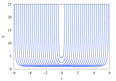
(a)

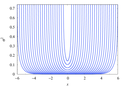
(b)

Figure 1: The functions $\lambda(x)$ (left) and $\sigma^{2}(x)$ (right) which are solutions to the gap equation, Eq. (2.6), for various values of $L$ ranging $L=1\sim 12$. $\Lambda=1$ in this figure. The innermost (outermost) curve corresponds to $L=1$ ($L=12$).

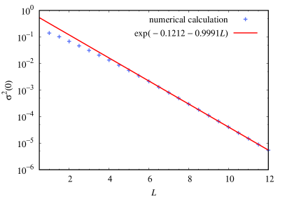
(a)

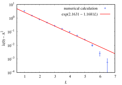
(b)

Figure 2: The values of fields in the middle of the interval $\sigma^{2}(0)$ and $\lambda^{2}(0)-\Lambda^{2}$ in a logarithmic plot. $\Lambda=1$ in this figure. These figures are just an illustration of the exponential behavior of $\sigma^{2}(0)$ and $\lambda^{2}(0)-\Lambda^{2}$ as functions of $L$, and are not intended to be precise fits to theory. Especially the numerical errors are quite large at large $L$ in the right figure (but still much smaller than $\Lambda^{2}=1$).

In Figure 3 we show the solutions in the interval $(-\frac{L}{2},0)$ by keeping one boundary fixed at $-\frac{L}{2}$. This clearly shows the convergence at large $L$ to the half-line solution $(-\infty,0]$.

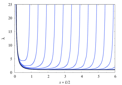
(a)

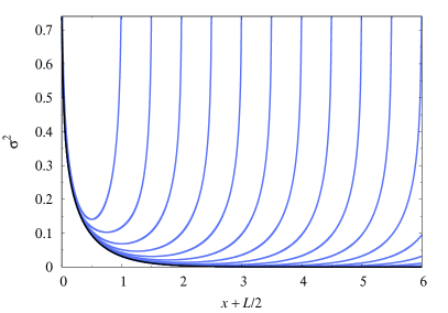
(b)

Figure 3: The function $\lambda(x)$ (left) and $\sigma^{2}(x)$ (right) which are the solutions of the gap equation, Eq. (2.6) in the interval $(-\frac{L}{2},0]$ for various values of $L$ ranging $L=1\sim 12$. $\Lambda=1$ in this figure.

As already noted in [3], one can clearly see that the asymptotic ($L\to\infty$) regime (with $\lambda(x)\sim\Lambda^{2}$ and $\sigma(x)\sim 0$ except near the boundaries) has already set in at $L\simeq 4$, which is quite reasonable ($L\Lambda=4\gg 1$). The effect of the boundaries is seen to propagate only for $\Delta x\sim 1/\Lambda$ from the latter: the system effectively reduces to the standard 2D ${\mathbb{C}P}^{N-1}$ model in an infinite spacetime, as one moves away from the boundaries by $\sim 1/\Lambda$ or more, as expected on general grounds.

2.2 $L$ dependence, near-the-boundary behavior of $\lambda(x),\sigma(x)$, and the classical limit

Our system has two parameters, the dynamically generated mass scale $\Lambda$ and the interval length $L$. But as $\Lambda$ fixes the physical unit of length, the model actually possesses only one parameter: what distinguishes two physically distinct systems is the product $\Lambda L$. The crucial point is that the UV divergences are short-distance effects around any fixed space point, and are universal. They do not depend on the presence or absence of the boundaries. This is what allows us to define unambiguously systems of “different space width $L$”.

The near-the-boundary behavior (2.12) can be obtained [3] as follows. Under the assumption (2.11), the large $n$ modes are given at any fixed $x$ by

$$f_{n}\simeq\sqrt{\frac{2}{L}}\sin\left(\frac{n\pi(x+L/2)}{L}\right)\;,\qquad\omega_{n}\simeq\frac{n\pi}{L}\;,\qquad n\gg 1\;.$$ (2.13)

The finite part of the sum over modes in the gap equation behaves then as

$$\frac{N}{2}\,\sum_{n}\frac{1}{\omega_{n}}\left(f_{n}(x)^{2}-\frac{1}{L}\right)=\frac{N}{2\pi}\log\left(2\sin{\left(\frac{\pi(x+L/2)}{L}\right)}\right)\simeq\frac{N}{2\pi}\log\left(\frac{2\pi}{L}(x+L/2)\right)\;,$$ (2.14)

near the left boundary. This singularity can only be compensated by $\sigma(x)^{2}$ in the gap equation, hence Eq. (2.12). The numerical solutions found in [3] and here clearly exhibit this logarithmic behavior.

There is an alternative way of understanding the behavior of $\sigma(x)$ and $\lambda(x)$ near the boundaries. Consider the regularized but un-renormalized form of the gap equation (2.6). By keeping the UV regularization parameter $\epsilon$ fixed and by going to $x=\mp\tfrac{L}{2}$, one finds that

$$\sigma\!\left(\mp\tfrac{L}{2}\right)^{2}=r_{\epsilon}=\frac{N}{2\pi}\log\left(\frac{1}{\epsilon}\right)+\cdots\;,$$ (2.15)

as $f_{n}=0$. This is nothing but the classical ${\mathbb{C}P}^{N-1}$ model (2.2) with the Dirichlet boundary condition

$$n_{1}\!\left(-\tfrac{L}{2}\right)=n_{1}\!\left(\tfrac{L}{2}\right)=\sqrt{r}\;,\qquad n_{i}\!\left(-\tfrac{L}{2}\right)=n_{i}\!\left(\tfrac{L}{2}\right)=0\;,\quad i>1\;.$$ (2.16)

With $x$ close to but not exactly at a boundary, $\epsilon$ in (2.15) is replaced by $\left|x\pm\tfrac{L}{2}\right|$ and one finds Eq. (2.12). This statement requires an explanation. What really happens is that in the gap equation (2.6), $\log 1/\epsilon$ which is in $\sigma(x)$ at exactly $x=-L/2$, is moved at small but nonvanishing $|x+L/2|$ to the first term involving the sum over the modes. After $\log 1/\epsilon$ is eliminated by the bare coupling constant term $r_{\epsilon}$ and the gap equation is renormalized and made finite, it produces $-\log 1/|x+L/2|$, which can only be compensated by $\sigma(x)^{2}$, as in (2.12). See Eq. (A.2) and Eq. (A.8).

This discussion clearly shows that the origin of the singular behavior of the mass gap $\lambda(x)$ and of the $\sigma(x)$ field is the fact that the system reduces to its classical limit near the boundaries, not having sufficient 2D spacetime volume for the $n_{i}$ fields to fluctuate.

The same reasoning explains the behavior of the value of $\lambda(x)$ and $\sigma(x)$ at the midpoint of the string at small $L\ll 1/\Lambda$, found in [3] (see Fig. 3 there),

$$\lambda(0)\sim\frac{4}{L^{2}}\log\frac{1}{L}\;,\qquad\sigma^{2}(0)\sim\frac{N}{2\pi}\log\frac{1}{L}\;.$$ (2.17)

3 Anomalous functional variation and the generalized gap equation

We now re-derive the generalized gap equation. Our starting point is the energy density

$${\cal E}(x) = \frac{N}{2}\sum_{n}\left(\omega_{n}f_{n}(x)^{2}+\frac{1}{\omega_{n}}\left(f^{\prime}_{n}(x)^{2}+\lambda f_{n}(x)^{2}\right)\right)e^{-\epsilon\omega_{n}}$$ (3.1)

$$\mathop{+}\sigma^{\prime}(x)^{2}+\lambda(x)\left(\sigma(x)^{2}-r_{\epsilon}^{0}\right)+{\cal E}_{\rm uv}\;,$$

where $\epsilon$ has been introduced as a regulator of the UV divergences coming from higher modes, ${\cal E}_{\rm uv}$ is a subtraction constant and $f_{n}(x)$, $\omega_{n}$ are the eigenmodes of the $n_{i}$ field equations

$$-f^{\prime\prime}_{n}(x)+\lambda(x)f_{n}(x)=\omega_{n}^{2}f_{n}(x)\;,\qquad\int_{-L/2}^{L/2}dx\;f_{n}(x)f_{m}(x)=\delta_{n,m}\;.$$ (3.2)

By integrating Eq. (3.1) over $x\in\left[-\tfrac{L}{2},\tfrac{L}{2}\right]$ and by using (3.2), one has the expression for the integrated energy,

$$E \equiv \int_{-L/2}^{L/2}dx\;{\cal E}(x)$$ (3.3)

$$= N\sum_{n}\omega_{n}e^{-\epsilon\omega_{n}}+\int_{-L/2}^{L/2}dx\left[\sigma^{\prime}(x)^{2}+\lambda(x)(\sigma(x)^{2}-r_{\epsilon}^{0})+{\cal E}_{\rm uv}\right]\;.$$

For instance the total derivative terms vanish as [3]

$$\lim_{x\to-L/2}f_{n}(x)f_{n}^{\prime}(x)=\lim_{x\to-L/2}\left(\frac{x+L/2}{-\log(x+L/2)}+{\cal O}\left(\frac{x+L/2}{2\log^{2}(x+L/2)}\right)\right)=0\;,\quad\forall n\;.$$ (3.4)

By varying (3.3) with respect to $\lambda(x)$, and by using

$$\delta\omega_{n}^{2}=\int_{-L/2}^{L/2}dx\;\delta\lambda(x)f_{n}(x)^{2}\,,\qquad\frac{\delta\omega_{n}}{\delta\lambda(x)}=\frac{f_{n}(x)^{2}}{2\omega_{n}}\,,$$ (3.5)

one gets the generalized gap equation

$$\frac{N}{2}\,\sum_{n}\frac{f_{n}(x)^{2}}{\omega_{n}}e^{-\epsilon\omega_{n}}+\sigma(x)^{2}-r_{\epsilon}=0\,,$$ (3.6)

where

$$r_{\epsilon}=r_{\epsilon}^{0}+\frac{N}{2\pi}\;,$$ (3.7)

whereas the variation with respect to $\sigma$ gives

$$\partial_{x}^{2}\sigma(x)-\lambda(x)\sigma(x)=0\ .$$ (3.8)

Note the extra $\frac{N}{2\pi}$ term in (3.7). It arises when the variation $\delta/\delta\lambda(x)$ acts on the regulator factor $e^{-\epsilon\omega_{n}}$:

$$N\sum_{n}\omega_{n}\frac{\delta}{\delta\lambda(x)}e^{-\epsilon\omega_{n}}=-\frac{\epsilon N}{2}\sum_{n}f_{n}(x)^{2}e^{-\epsilon\omega_{n}}:$$ (3.9)

this term is superficially of the order of $\mathcal{O}(\epsilon)$: however the sum in the last expression diverges as $\frac{1}{\epsilon}$, so it gives a nonvanishing contribution . As the divergence comes from large $n$ it may be calculated as

$$-\frac{\epsilon N}{2}\sum_{n}f_{n}^{2}(x)e^{-\epsilon\omega_{n}}\simeq-\frac{\epsilon N}{2L}\sum_{n}\left[1-\cos\left(\frac{2n\pi(x+L/2)}{L}\right)\right]e^{-\epsilon\pi n/L}\;=-\frac{N}{2\pi}+\mathcal{O}(\epsilon)\;,$$ (3.10)

for

$$-\tfrac{L}{2}<x<\tfrac{L}{2}\;,$$ (3.11)

where use was made of an approximate form for the eigenmodes

$$f_{n}\simeq\sqrt{\frac{2}{L}}\sin\left(\frac{n\pi(x+L/2)}{L}\right)\;,\qquad\omega_{n}\simeq\frac{n\pi}{L}\;,\qquad n\gg 1\;.$$ (3.12)

The same result can be found by using the propagator representation (2.9). See Appendix A.2.

4 Energy density

We now go back to the density itself, and rewrite (3.1) as

$${\cal E}(x) = {\cal E}_{0}(x)+\lambda(x)\left(\frac{N}{2}\sum_{n}\frac{1}{\omega_{n}}f_{n}(x)^{2}+\sigma(x)^{2}-r_{\epsilon}^{0}\right)+{\cal E}_{\rm uv}\;$$ (4.1)

$$= {\cal E}_{0}(x)+\frac{N}{2\pi}\lambda(x)+{\cal E}_{\rm uv}\;,$$

where

$${\cal E}_{0}(x)\equiv\frac{N}{2}\sum_{n}\left(\omega_{n}f_{n}(x)^{2}+\frac{1}{\omega_{n}}f^{\prime}_{n}(x)^{2}\right)e^{-\epsilon\omega_{n}}+\sigma^{\prime}(x)^{2}\;,$$ (4.2)

by collecting terms proportional to $\lambda(x)$ and by using Eqs. (3.6) and (3.7). Note that the anomaly (3.7) is crucial to give the term proportional to $\lambda(x)$ in the energy density, after using the gap equation.

It turns out that ${\cal E}_{0}(x)$ is a constant. The space derivative of ${\cal E}_{0}(x)$ is:

$$\frac{d{\cal E}_{0}(x)}{dx} = N\sum_{n=1}^{\infty}\left(\omega_{n}f_{n}f^{\prime}_{n}+\frac{1}{\omega_{n}}f^{\prime}_{n}f^{\prime\prime}_{n}\right)e^{-\epsilon\omega_{n}}+2\sigma^{\prime}\sigma^{\prime\prime}\;$$ (4.3)

$$= N\sum_{n=1}^{\infty}\left(\omega_{n}f_{n}f^{\prime}_{n}+\frac{1}{\omega_{n}}f^{\prime}_{n}(\lambda-\omega_{n}^{2})f_{n}\right)e^{-\epsilon\omega_{n}}+2\sigma^{\prime}(\lambda\sigma)\;$$

$$= \lambda(x)\left[N\sum_{n=1}^{\infty}\frac{1}{\omega_{n}}f_{n}f^{\prime}_{n}e^{-\epsilon\omega_{n}}+2\sigma\sigma^{\prime}\right]\;.$$

Noting that the expression in the square bracket above is the derivative of the gap equation (3.6), we conclude that

$$\frac{d{\cal E}_{0}(x)}{dx} = 0\ .$$ (4.4)

We thus find that the energy density is

$${\cal E}(x,\Lambda,L)={\cal E}_{0}(\Lambda,L)+\frac{N}{2\pi}\lambda(x,\Lambda,L)+{\cal E}_{\rm uv}\;,$$ (4.5)

where the only dependence on $x$ is through the function $\lambda(x)$.

Let us study the $L\to\infty$ limit of this expression. The value of the constant part of the energy density, ${\cal E}_{0}$, in the $L\to\infty$ limit may be calculated by noting that $\lambda(x)\to\Lambda^{2}$ and the fact that the spectrum is exactly known in that limit. See Appendix B. The result is

$${\cal E}_{0}(\Lambda,L=\infty)=\frac{N}{\pi\epsilon^{2}}-\frac{N\Lambda^{2}}{4\pi}\;.$$ (4.6)

This shows that the energy density of the system, after the standard regularization and renormalization of the coupling constant has been made to render the gap equation finite, still contains a quadratic divergence. This is a little similar to the vacuum density in QCD: the theory can be renormalized and all physical quantities can be calculated order by order in perturbation theory, but the vacuum energy density (a contribution to the cosmological constant) is still divergent, and requires a further subtraction. The result (4.6) however suggests that we take the vacuum energy subtraction constant simply as

$${\cal E}_{\rm uv}=-\frac{N}{\pi\epsilon^{2}}\;,$$ (4.7)

and the constant part of the energy density is thus

$${\cal E}_{0}(\Lambda,L=\infty)+{\cal E}_{\rm uv}=-\frac{N\Lambda^{2}}{4\pi}\;.$$ (4.8)

As

$$\lambda(x,\Lambda,L)\to\Lambda^{2},\qquad\forall x,\quad x\neq\pm\frac{L}{2},\qquad L\to\infty\;,$$ (4.9)

one finds that the total energy density approaches a constant

$${\cal E}(x,\Lambda,L=\infty)=\frac{N}{4\pi}\Lambda^{2}\;,$$ (4.10)

at any fixed finite $x$. This gives the quantum corrections due to the fluctuations of the $n_{i}$ fields to the classical ”tension” of the vortex, $\xi\,$, where $\Lambda^{2}\ll\xi\,.$ This result is in agreement with the one [12], found in a finite worldstrip ${\mathbb{C}P}^{N-1}$ model with periodic boundary conditions.

As we shall see in the next section, and as can be verified by a WKB analysis done in Appendix D, the divergence in the energy density remains purely quadratic: the only subtraction needed is (4.7), in the case of finite ($L$) string also. No linear or logarithmic divergences are present. This is reasonable as the divergences due to the fluctuations of the $n_{i}$ fields is a short-distance effect, local in $x$, and cannot depend on the presence of the boundaries.

5 Large but finite $L$: an Ansatz and analytic calculation

We now study the corrections to (4.9) and (4.10) (and $\sigma(0)=0$) for large but finite $L$. In order to do that, it is clearly necessary to analyze the large-$L$ behavior of (the solution of) the gap equation, (3.6), (3.8) itself. To start with, $\lambda(x,\Lambda,L)$ can be approximately taken to be a constant for $|x|\ll L/2$; we parametrize its asymptotic approach to $\Lambda^{2}$ as

$$\lambda(0,\Lambda,L)=\tilde{\Lambda}^{2}\equiv\Lambda^{2}e^{2a},\qquad\lim_{L\to\infty}a(\Lambda L)=0\;.$$ (5.1)

The factor $a$ represents the nonlocal effect due to the boundary condition. To estimate this, consider the propagator, Eq. (2.9). For $x,x^{\prime}\sim 0$ (i.e., far from the boundaries), it satisfies locally

$$\left(\partial_{\epsilon}^{2}+\partial_{x}^{2}-\tilde{\Lambda}^{2}\right)D(x,\epsilon;x^{\prime},0)\sim\delta(\epsilon)\delta(x-x^{\prime})\;,$$ (5.2)

thus its solution can be assumed to have the form

$$D(x,\epsilon;x^{\prime},0) \sim \frac{1}{2\pi}K_{0}\big{(}\tilde{\Lambda}\sqrt{(x-x^{\prime})^{2}+\epsilon^{2}}\big{)}$$ (5.3)

$$-\frac{A}{2\pi}\left(K_{0}\big{(}\tilde{\Lambda}\sqrt{(x+x^{\prime}+L)^{2}+\epsilon^{2}}\big{)}+K_{0}\big{(}\tilde{\Lambda}\sqrt{(L-x-x^{\prime})^{2}+\epsilon^{2}}\big{)}\right)$$

$$+\cdots$$

with an unknown constant $A=A(\Lambda L)$. The subleading terms in the second line come from the nearest mirror poles in Eq. (2.10). It is expected that $A=A(\Lambda L)\sim\mathcal{O}(1)$, but due to the effects of the boundaries where $\lambda(x)$ is non constant and singular [3] it will not coincide with the exact value $A=1$ (for the Dirichlet boundary condition at $x=\pm L/2$) or $A=-1$ (for the Neumann boundary condition) (cfr. Eq. (A.1)) [3].

The gap equation (3.6) then yields near $x=0$

$$\sigma^{2}(x) \sim \frac{N}{2\pi}\log\frac{\tilde{\Lambda}}{\Lambda}+\frac{NA}{2\pi}\left(K_{0}\big{(}2\tilde{\Lambda}(x+L/2)\big{)}+K_{0}\big{(}2\tilde{\Lambda}(L/2-x)\big{)}\right)$$ (5.4)

$$\simeq \frac{N}{2\pi}a+\frac{NA}{\pi}K_{0}(\tilde{\Lambda}L)+\frac{2NA\tilde{\Lambda}^{2}}{\pi}K_{0}^{\prime\prime}(\tilde{\Lambda}L)\,x^{2}+\cdots$$

Equation (3.8) gives $\lambda(x)$ near $x=0$ ($\sigma^{\prime}\simeq 0$):

$$\lambda(x)=\frac{\sigma^{\prime\prime}(x)}{\sigma(x)}\sim\frac{(\sigma(x)^{2})^{\prime\prime}}{2\,\sigma(x)^{2}}\sim\tilde{\Lambda}^{2}\frac{2AK_{0}^{\prime\prime}}{a/2+AK_{0}}\;.$$ (5.5)

By requiring the consistency of this with the initial Ansatz (5.1) and making use of the identity

$$K_{0}(x)+K_{2}(x)=2K_{0}^{\prime\prime}(x)\;,$$ (5.6)

one finds that

$$a=2A\,K_{2}(\tilde{\Lambda}L)=2A\,K_{2}(\Lambda Le^{a})\simeq 2A\,K_{2}(\Lambda L)\;,$$ (5.7)

and

$$\tilde{\Lambda}^{2}\equiv\Lambda^{2}e^{2a}\simeq\Lambda^{2}(1+2a)\sim\Lambda^{2}\left(1+4AK_{2}(\Lambda L)\right)\;.$$ (5.8)

Thus one finds at large $L\gg\tfrac{1}{\Lambda}$ that, around $x=0$,

$$\lambda(x,\Lambda,L) \sim \lambda(0,\Lambda,L)\sim\Lambda^{2}\left(1+4AK_{2}(\Lambda L)\right),$$

$$\sigma^{2}(x,\Lambda,L) \sim \frac{2NA}{\pi}K_{0}^{\prime\prime}(\Lambda L)\left(1+\Lambda^{2}x^{2}\right)\;.$$ (5.9)

With these results in hand, one can now calculate the asymptotic behavior of the energy density itself:

$${\cal E}(x,\Lambda,L)={\cal E}_{0}(\Lambda,L)+\frac{N}{2\pi}\lambda(x,\Lambda,L)+{\cal E}_{\rm uv}\;.$$ (5.10)

It turns out under the same approximation (5.3) that the constant part of the energy density, ${\cal E}_{0}(\Lambda,L)$, is given at finite large $L$ by

$${\cal E}_{0}(\Lambda,L)\sim\frac{N}{\pi\epsilon^{2}}-\frac{N\Lambda^{2}}{4\pi}-\frac{NA\Lambda^{2}}{\pi}\left(K_{0}(\Lambda L)+K_{2}(\Lambda L)\right)+{\cal O}(e^{-2\Lambda L})\;.$$ (5.11)

The derivation of this result is given in Appendix C. Note that the divergence in the energy density is just the purely quadratic one, $\frac{N}{\pi\epsilon^{2}}$, the same as in the $L\to\infty$ case discussed in the previous section. This is correct, as the divergences arise from the UV fluctuations of the $n_{i}$ fields which is a local effect, independent of the boundaries, or of the value of $L$.

Finally one finds, by adding the $\lambda(0,\Lambda,L)$ term and by making the same subtraction as before, viz. (4.7),

$${\cal E}(0,\Lambda,L) = \frac{N}{2\pi}\lambda(0,\Lambda,L)+{\cal E}_{0}(\Lambda,L)+{\cal E}_{\rm uv}$$ (5.12)

$$\sim \frac{N\Lambda^{2}}{4\pi}+\frac{NA\Lambda^{2}}{\pi}(K_{2}(\Lambda L)-K_{0}(\Lambda L))+{\cal O}(e^{-2\Lambda L})$$

$$= \frac{N\Lambda^{2}}{4\pi}+\frac{2NA\Lambda}{\pi L}K_{1}(\Lambda L)+{\cal O}(e^{-2\Lambda L})\;,$$

where another identity

$$K_{2}(x)-K_{0}(x)=2K_{1}(x)/x\;,$$ (5.13)

has been used.

To conclude, we find that the approach to the asymptotic value of the energy density is exponential: no pure power corrections in $1/L$ (i.e. the Lüscher term) are present. This is perfectly consistent with the general result found in [3] that our system has a unique phase, which smoothly matches – in the large $L$ limit – the “confinement phase” of the standard 2D ${\mathbb{C}P}^{N-1}$ model. All $n_{i}$ ($i\neq 1$) fields gain a dynamically generated mass $\sim\Lambda$; at the same time $\sigma\sim 0$ except at the boundaries. In other words, no dynamical breaking of the isometry group $SU(N)$ takes pace. No Nambu-Goldstone modes associated with the internal, orientational modes are generated. The absence of a long-range correlation in the large-$L$ corrections in Eqs. (5.9), (5.12) is a simple reflection of this fact.

6 Numerical results

Due to the quadratic divergence present in the sum (4.2) the numerical calculation turns out to present quite a bit of a challenge. Any tiny errors in the eigenmodes and in the energy levels will introduce linear or logarithmic divergences in the sum, and the finite answer for ${\cal E}(x,\Lambda,L)$ one gets (including its dependence on $x$, $L$ and $\Lambda$) depends on how these fake divergences are appropriately subtracted, together with the genuine quadratic divergences. Because of this, even the best results so far do not have a precision comparable to the solution of the generalized gap equation discussed in Section 3.

The check of the constancy of ${\cal E}_{0}$, is shown in Fig. 4. Note that it is found indeed to be constant everywhere, including values of $x$ very close to the boundaries, where the distances from the latter are much smaller than $1/\Lambda$. Fig. 6 shows the value of ${\cal E}_{0}$ as a function of $L$ ($\Lambda=1$). The total energy density, including the $N\lambda(x)/2\pi$ term, calculated at the midpoint, $x=0$, is shown in Fig. 6. The numerical results are nicely consistent with the exact result at $L=\infty$, and with the analytic behavior for large but finite $L$, found in the previous section, with $A\sim 1$. ${\cal E}_{0}$ and ${\cal E}(0,\Lambda,L)$ are plotted against $\Lambda$ at fixed $L$, in Fig. 8 and in Fig. 8. In particular we see that as $\Lambda\to 0$ the energy density converges, although quite slowly (i.e. logarithmically), to the free-field value $-\pi/12L^{2}$.

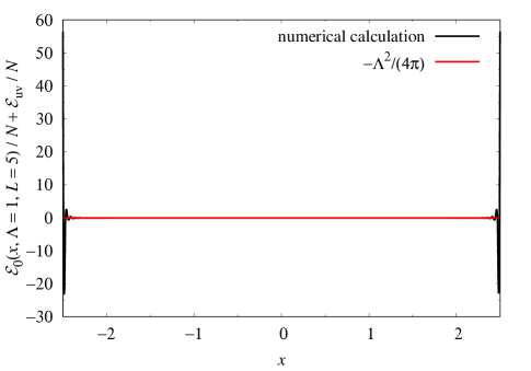
Figure 4: Verification of the constancy of $({\cal E}_{0}+{\cal E}_{\rm uv})$ with respect to $x$. $\Lambda=1$, $L=5$ in this figure.

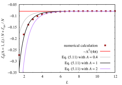
Figure 5: The constant part of the energy density, ${\cal E}_{0}+{\cal E}_{\rm uv}$, is plotted as a function of $L$ for $\Lambda=1$ fixed.

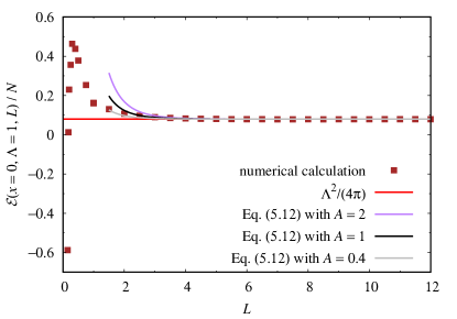
Figure 6: The total energy density at the midpoint, ${\cal E}$, is plotted against $L$ for $\Lambda=1$ fixed.

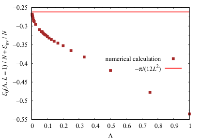
Figure 7: The constant part of the energy density, ${\cal E}_{0}+{\cal E}_{\rm uv}$, is plotted as a function of $\Lambda$ for $L=1$ fixed.

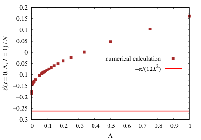
Figure 8: The total energy density at the midpoint, ${\cal E}$, is plotted against $\Lambda$ for $L=1$ fixed.

7 Boundary divergence and the Casimir force

The energy density

$${\cal E}(x,\Lambda,L)={\cal E}_{0}(\Lambda,L)+\frac{N}{2\pi}\lambda(x,\Lambda,L)+{\cal E}_{\rm uv}\;,$$ (7.1)

after renormalization is a finite function of $x,\Lambda,L$. When integrated over $x\in\left[-\frac{L}{2},\frac{L}{2}\right]$, it gives the total energy of the string

$$E(\Lambda,L) = \int_{-L/2}^{L/2}dx\;{\cal E}(x,\Lambda,L)=\int_{-L/2}^{L/2}dx\,\left[{\cal E}_{0}(\Lambda,L)+\frac{\lambda(x,\Lambda,L)}{2\pi}\right]$$ (7.2)

$$= L\,{\cal E}_{0}(\Lambda,L)+\int_{0}^{L/2}dx\;\frac{\tilde{\lambda}(x,\Lambda,L)}{\pi}\;,$$

where we introduced the mass gap function defined on the interval $[0,L]$,

$$\tilde{\lambda}(x,\Lambda,L)\equiv\lambda(x-L/2,\Lambda,L)\,.$$ (7.3)

The Casimir force is defined as

$$F=\frac{\partial E(\Lambda,L)}{\partial L}\;.$$ (7.4)

Before analyzing the behavior of $F$ for various values of $L$, let us note that the second term in Eq. (7.2) gives rise to a new divergence in the integrated energy due to the singular behavior near the boundaries, e.g., near $x=0$,

$$\tilde{\lambda}(x)\sim\frac{1}{x^{2}\log 1/(x\Lambda)}\;,\qquad L\gg 1/\Lambda\gg x\;.$$ (7.5)

As $\tilde{\lambda}(x)$ quickly approaches the constant value $\Lambda^{2}$ beyond $x\simeq 1/\Lambda$, for sufficiently large $L$, the divergent part can be extracted by considering the finite integral

$$E_{1}=\frac{N}{2\pi}\int_{\epsilon}dx\;(\tilde{\lambda}(x)-\Lambda^{2})\sim\frac{N}{2\pi}\frac{1}{\epsilon\log{1/\epsilon\Lambda}}\simeq\frac{N}{2\pi\epsilon}\frac{Ng(\epsilon)^{2}}{8\pi^{2}}\;,$$ (7.6)

where a UV cutoff ($x=\epsilon$) has been introduced. Similarly $E_{2}$ for the contribution from the right boundary. $E_{1}$ ($E_{2}$) is an energy concentrated at the left (right) boundary: it can be interpreted as the quantum corrections to the monopole (antimonopole) mass, due to the $n_{i}$ field fluctuations (the factor $N$). $E_{1,2}$ can be subtracted (i.e., compensated with the bare mass terms) from the total energy, leaving finite, renormalized monopole masses. They do not affect the discussion on the $L$ dependent Casimir effect below.

The Casimir force can be rewritten, by differentiating Eq. (7.2), as

$$F = {\cal E}_{0}(\Lambda,L)+L\,\frac{\partial{\cal E}_{0}(\Lambda,L)}{\partial L}+\frac{\lambda(0,\Lambda,L)}{2\pi}+\frac{1}{\pi}\int_{0}^{L/2}dx\,\frac{\partial\tilde{\lambda}(x,\Lambda,L)}{\partial L}$$ (7.7)

$$= {\cal E}(0,\Lambda,L)+L\,\frac{\partial{\cal E}_{0}(\Lambda,L)}{\partial L}+\frac{1}{\pi}\int_{0}^{L/2}dx\,\frac{\partial\tilde{\lambda}(x,\Lambda,L)}{\partial L}\;.$$

Note that this is a finite quantity since it is not sensitive to the leading divergence of $\tilde{\lambda}$, viz. (7.5).

At very small $L$ (i.e. $L\Lambda\ll 1$) one expects the dominant effect to come from the second term of (7.7) (see Fig. 8):

$$F\simeq L\,\frac{\partial{\cal E}_{0}(\Lambda,L)}{\partial L}\simeq\frac{N\pi}{6L^{2}}\;:$$ (7.8)

it is an attractive free-field Casimir force.

At intermediate values, $L\sim\mathcal{O}(1/\Lambda)$, instead, we find that the force is dominated by the third term in (7.7). The strong decrease ($\sim 1/L^{2}\log(1/L)$) of the mass gap $\tilde{\lambda}(x)$ with $L$ for all $x$ (see e.g., Eq. (2.17)) cannot be compensated by a linear effect of integration, therefore there is an effective repulsive force at work. The total energy of the system is lowered when the space interval $L$ gets larger.

At sufficiently large $L$, $L\gg 1/\Lambda$, where the $2D$ regime sets in, the leading contribution comes from the first term in (7.7):

$$F\simeq{\cal E}(0,\Lambda,L)\simeq\frac{N\Lambda^{2}}{4\pi}\;,$$ (7.9)

corresponding to an approximately constant string tension (Eq. (4.10)). An external observer who attempts to pull the boundaries further apart will experience an attractive, constant force countering her/him.

A precise numerical verification of this nontrivial behavior of the force turned out to be exceedingly difficult because of the singular behavior of $\lambda(x)$ near the boundaries. Our preliminary result (not shown) however clearly confirms the change from a repulsive regime at $L=\mathcal{O}(1/\Lambda)$ to an attractive force at $L\gg 1/\Lambda$.

8 Conclusion

In this paper we have examined the energy density function ${\cal E}(x,\Lambda,L)$ of the large-$N$ $\mathbb{C}P^{N-1}$ sigma model on a finite string, defined with the Dirichlet boundary conditions. We find that it is a sum of two terms, the first expressed as a sum over fluctuation modes, which turns out to be constant in $x$, and the second term proportional to the mass gap $\lambda(x)$. The only $x$ dependence arises from the second. The first term is quadratically divergent, analogous to the vacuum energy in QCD. The $L$-dependence of ${\cal E}(x,\Lambda,L)$ at fixed $\Lambda$ shows that the effect of the boundaries are limited to their vicinity of width $\sim 1/\Lambda$: the system approaches quickly the standard 2D large-$N$ $\mathbb{C}P^{N-1}$ sigma model, with dynamical generation of the mass gap, and with no dynamical breaking of the isometry group $SU(N)$. In the small $L\Lambda$ limit, the system approaches the classical weakly-coupled $\mathbb{C}P^{N-1}$ model, as appropriate for the Dirichlet boundary conditions.

The approach to the limit ${\cal E}(x,\Lambda,L=\infty)=\tfrac{N}{4\pi}\Lambda^{2}$ is found to be purely exponential: no power corrections in $1/L$ such as the Lüscher term are present. This is perfectly consistent with the general result found in [3] that our system has a unique phase, which smoothly matches the “confinement phase” in the large-$L$ limit of the standard 2D ${\mathbb{C}P}^{N-1}$ model. All $n_{i}$ ($i\neq 1$) fields gain a dynamically generated mass $\sim\Lambda$; at the same time $\sigma\sim 0$ except at the boundaries. In other words, no dynamical breaking of the isometry group $SU(N)$ takes pace, and no associated Nambu-Goldstone modes are generated. The absence of the long-range correlation reflects this fact.

Recently a paper appeared [16] in which some analytical large-$N$ $\mathbb{C}P^{N-1}$ sigma model solutions for inhomogeneous condensates are presented by a mapping to the Gross-Neveu model [15]. These solutions correspond to periodic boundary conditions and, as far as we can see, none of the solutions proposed there correspond to our system defined with the Dirichlet boundary conditions. It would certainly be very interesting if our type of solution could be found analytically with developments of these techniques in the future.

Acknowledgments

We thank Jarah Evslin, Muneto Nitta, Misha Shifman and Ryosuke Yoshii for discussions. The work of S. B. is funded by the grant “Rientro dei Cervelli Rita Levi Montalcini” of the Italian government. The work of S. B. G. was supported by the National Natural Science Foundation of China (Grant No. 11675223). K. O. is supported by the Ministry of Education, Culture, Sports, Science (MEXT)-Supported Program for the Strategic Research Foundation at Private Universities “Topological Science” (Grant No. S1511006) and by the Japan Society for the Promotion of Science (JSPS) Grant-in-Aid for Scientific Research (KAKENHI Grant No. 16H03984). The present research work is supported by the INFN special research project grant, GAST (“Gauge and String Theories”).

When this paper was being prepared for submission we were informed by Muneto Nitta and Ryosuke Yoshii of their paper [17], which deals with similar problems as ours, and with some overlap. The boundary behavior for the gap function and some other qualitative aspects of their solutions are different from ours. Also, another paper [18] just appeared, discussing a Grassmannian sigma model on finite-width world sheets.

Comments on Ref. [17]

In Ref. [17], submitted to the ArXiv on the same day as ours, the same system is analyzed in a different approach, and the authors there claim to find analytic solutions for mass gap function $\lambda(x)$ and for $\sigma(x)$, both in confinement and in Higgs phases.

By imposing Dirichlet boundary conditions and solving the generalized gap equations, we instead find the solutions (e.g., illustrated in Fig. 1) in a unique phase with mass gap for all values of $L$, which smoothly approaches the well-known solution in the infinite $L$ limit (the standard $2D$ ${\mathbbm{C}}P^{N-1}$ model). Our solutions are moreover consistent with the classical ${\mathbbm{C}}P^{N-1}$ model in the $L\ll 1/\Lambda$ limit as discussed in Sec. 2.2.

It is possible that, if a Higgs-like solution (as in Fig. 1(b) of [17]) would exist, it represents an unstable solution, whereas our procedure necessarily picks up the stable solution, and that actually the confinement-type solution is always the stable one.

However, we find it difficult to make a proper comparison, as the renormalization of the gap equation and the generation of the mass scale $\Lambda$ are not explained in [17].

The boundary behavior of the mass gap function and the field $\sigma$ given in [17] is powerlike, whereas the logarithmic behavior found by us reflects the situation characteristic of a finite-space-width system. The system must compromise between the $2D$ physics at $L\geq 1/\Lambda$ - the divergences of the $n_{i}$ field fluctuations and the generation of the mass scale $\Lambda$ - and the classical limit to which the model must reduce correctly in the $L\ll 1/\Lambda$ region, as explained in Sec. 2.2.

As the physical values of $L$ (the space width) are not given in reference to $1/\Lambda$ in [17], in contrast to what is done in the present paper, it is not clear to us which physical values of $L$ their solutions in Fig. 1(b) or Fig. 1(a) refer to, for instance.

As a consequence, it is unclear how and when (at which value of $L$) the Higgs phase vacuum disappears, as $L$ is increased. Or, vice versa, at which $L$, if $L$ decreases toward zero, the Higgs vacuum takes over, if it does at all. The authors of [17] do not give the criteria to decide which solutions should be chosen at any given $L$. As far as we can see, the analysis of the vacuum energy density, as made in the present paper, has not been done yet there.

Appendix A Propagator $D(x,\tau;x^{\prime},\tau^{\prime})$

A.1 Exact forms with $\lambda(x)=m^{2}$

When $\lambda(x)=m^{2}$, Eq. (2.10) can be easily solved by

$$D(x,\tau;x^{\prime},\tau^{\prime}) = \sum_{n\in Z}\frac{1}{2\pi}K_{0}\big{(}m\sqrt{(x-x^{\prime}+2nL)^{2}+(\tau-\tau^{\prime})^{2}}\big{)}$$ (A.1)

$$-\sum_{n\in Z}\frac{1}{2\pi}K_{0}\big{(}m\sqrt{(x+x^{\prime}+(2n+1)L)^{2}+(\tau-\tau^{\prime})^{2}}\big{)}\;,$$

for the Dirichlet-Dirichlet boundary condition (2.3). In particular, note that

$$D(x,\epsilon;x,0)=\sum_{n\in Z}\frac{1}{2\pi}K_{0}\big{(}m\sqrt{(2nL)^{2}+\epsilon^{2}}\big{)}-\sum_{n\in Z}\frac{1}{2\pi}K_{0}\big{(}m\sqrt{(2x+(2n+1)L)^{2}+\epsilon^{2}}\big{)}\;.$$ (A.2)

In the case of the Neumann-Neumann boundary condition (2.4), the sign of the last terms of the r.h.s. is flipped.

A.2 Alternative derivation of the anomalous functional variation

In terms of the propagator (2.9), the extra factor in Eq. (3.9) can be expressed as

$${\rm r.h.s.~{}of~{}Eq.(\ref{anvar})}=-\frac{\epsilon N}{2}\sum_{n}f_{n}(x)^{2}e^{-\epsilon\omega_{n}}=\epsilon N\frac{\partial}{\partial\epsilon}D(x,\epsilon;x,0).$$ (A.3)

Since the UV divergence comes from a short-distance effect, to extract divergent terms of $D(x,\epsilon,x,0)$, it is sufficient to consider the contribution of the nearest poles, $\delta(\tau-\tau^{\prime})\delta(x-x^{\prime})$ ($n=0$ term) in Eq. (2.10). Furthermore, at short distances $\lambda(x)(|x-x^{\prime}|^{2}+\epsilon^{2})\ll 1$, the potential $\lambda(x)$ can be omitted and thus the propagator behaves as one for a massless field in two dimensional space,

$$D(x,\epsilon;x^{\prime},0)\sim-\frac{1}{4\pi}\log\left(|x-x^{\prime}|^{2}+\epsilon^{2}\right)+{\rm regular~{}terms}.$$ (A.4)

With a general potential $\lambda(x)$, therefore, the divergent part of ${D}(x,\epsilon;x,0)$ (for $-\tfrac{L}{2}<x<\tfrac{L}{2})$ is universal as

$${D}(x,\epsilon;x,0)\sim-\frac{1}{2\pi}\log(\epsilon)+{\rm regular~{}terms}\,.$$ (A.5)

In the simplest case with $\lambda(x)=m^{2}$, one can easily check this property using Eq. (A.1) and $K_{0}(m\epsilon)\sim\log\tfrac{1}{\epsilon}$. We find

$$\lim_{\epsilon\to 0}\epsilon\frac{\partial}{\partial\epsilon}{D}(x,\epsilon;x,0)=-\frac{1}{2\pi},\qquad x\neq\pm\frac{L}{2}\;,$$ (A.6)

which gives the extra constant term $-\frac{N}{2\pi}$ in the gap equation.

Similarly, in a region where

$$\lambda(x)\left((x-x^{\prime})^{2}+\epsilon^{2}\right)\ll 1,\quad\lambda(x)\left((x+x^{\prime}\pm L)^{2}+\epsilon^{2}\right)\ll 1\;,$$ (A.7)

the dominant behavior of the propagator is

$$D(x,\epsilon;x^{\prime},0)\sim\frac{1}{4\pi}\log\left(|x+x^{\prime}\pm L|^{2}+\epsilon^{2}\right)-\frac{1}{4\pi}\log\left(|x-x^{\prime}|^{2}+\epsilon^{2}\right)+\cdots\;,$$ (A.8)

where $(\ldots)$ stands for regular terms. For instance, the two contributions in (A.8) exactly cancel each other at the boundaries $x=\pm L/2$, consistently with the boundary condition (2.3) for the eigenmodes.

Appendix B Calculation of ${\cal E}_{0}(\Lambda,L=\infty)$

At large $L$ and at finite $x$, where $\lambda(x)\sim\Lambda^{2}$, one can make an approximation valid at all levels $n$ (simply assume $\lambda=m^{2}=\Lambda^{2}$). Then

$${\cal E}_{0} = \frac{N}{2}\sum_{n=1}^{\infty}\left(\omega_{n}f_{n}(x)^{2}+\frac{1}{\omega_{n}}f^{\prime}_{n}(x)^{2}\right)e^{-\epsilon\omega_{n}}+(\sigma^{\prime}(x))^{2}\;,$$ (B.1)

with

$$f_{n}(x)=\sqrt{\frac{2}{L}}\sin\left(\frac{n\pi(x+L/2)}{L}\right),\qquad\omega_{n}=\sqrt{\left(\frac{n\pi}{L}\right)^{2}+m^{2}}\;,\qquad n\geq 1,\quad n\in\mathbb{Z}\;.$$ (B.2)

As ${\cal E}_{0}$ has been shown to be a constant, it can be calculated at any fixed $x$, for example at the midpoint $x=0$, where $\sigma^{\prime}=0$:

$$f_{n}(L/2)=\sqrt{\frac{2}{L}}\sin\left(\frac{n\pi}{2}\right)\;,\qquad f_{n}^{\prime}(L/2)=\sqrt{\frac{2}{L}}\frac{\pi n}{L}\cos\left(\frac{n\pi}{2}\right)\;.$$ (B.3)

In the $L\to\infty$ limit, the sum may be replaced by an integral, by $\frac{\pi n}{L}\to z$. Also, let us make a replacement

$$e^{-\epsilon\omega_{n}}\to e^{-\epsilon\pi n/L}\;,\qquad{\rm i.e.,}\qquad\omega_{n}=\sqrt{\left(\frac{n\pi}{L}\right)^{2}+\Lambda^{2}}\to\frac{n\pi}{L}\;,$$ (B.4)

in the exponential damping factor. One finds

$${\cal E}_{0}^{\prime} = \frac{N}{\pi}\int_{0}^{\infty}dz\,\left(\sqrt{z^{2}+\Lambda^{2}}\sin^{2}\tfrac{zL}{2}+\frac{z^{2}}{\sqrt{z^{2}+\Lambda^{2}}}\cos^{2}\tfrac{zL}{2}\right)e^{-\epsilon z}$$ (B.5)

$$\sim \frac{N\Lambda^{2}}{2\pi}\int_{0}^{\infty}dz\,\frac{2z^{2}+1}{\sqrt{z^{2}+1}}e^{-\epsilon z\Lambda}\;.$$

Now

$$\int_{0}^{\infty}dz\,\frac{2z^{2}+1}{\sqrt{z^{2}+1}}e^{-\epsilon z\Lambda}=\frac{2}{\epsilon^{2}\Lambda^{2}}+\frac{1}{2}+\mathcal{O}(\epsilon)\;,$$ (B.6)

therefore

$${\cal E}_{0}^{\prime}=\frac{N}{\pi\epsilon^{2}}+\frac{N\Lambda^{2}}{4\pi}\;.$$ (B.7)

In going from (B.1) to (B.5), however, we made a replacement (B.4) in the exponential damping factor. The correction due to this approximation must be taken into account. The effect of this replacement can be studied by writing

$${\cal E}_{0} = \frac{N}{2\pi}\int_{0}^{\infty}dz\,(\ldots)\,e^{-\epsilon z}e^{-\epsilon(\omega_{n}-z)}$$ (B.8)

$$= \frac{N}{2\pi}\int_{0}^{\infty}dz\,(\ldots)\,e^{-\epsilon z}\,\left[1-\epsilon(\omega_{n}-z)+\cdots\right]\;.$$

Clearly the terms of order $\epsilon^{2}$ or higher inside $[\ldots]$ are unimportant, as the integral in $z$ is finite without the regularizing exponential factor, or at most logarithmically divergent for the $\epsilon^{2}$ term. The $\mathcal{O}(\epsilon)$ term in the square bracket $[\ldots]$ gives

$$\epsilon\,\frac{N}{2\pi}\int_{0}^{\infty}dz\,(\ldots)\,(\omega_{n}-z)\,e^{-\epsilon z}\;,$$ (B.9)

but

$$\omega_{n}-z\sim\frac{1}{2z}\;,$$ (B.10)

and

$$(\ldots)\sim z\;,$$ (B.11)

(see (B.5)) so

$$(\ldots)\,(\omega_{n}-z)\sim 1\;,$$ (B.12)

at large $z$: the integral diverges linearly as

$$\int_{0}^{\infty}dz\,e^{-\epsilon z}\sim\frac{1}{\epsilon}\,$$ (B.13)

so it gives a finite contribution. It is

$$-\epsilon\frac{N\Lambda^{3}}{2\pi}\int_{0}^{\infty}dz\frac{2z^{2}+1}{\sqrt{z^{2}+1}}\left(\sqrt{z^{2}+1}-z\right)\,e^{-\epsilon\Lambda z}\;.$$ (B.14)

This can be easily calculated to give

$$-\frac{N\Lambda^{2}}{2\pi}+\mathcal{O}(\epsilon)\;.$$ (B.15)

This must be added to (B.7) obtained under the approximation (B.4): the final answer is

$${\cal E}_{0}(\Lambda,L=\infty)=\frac{N}{\pi\epsilon^{2}}-\frac{N\Lambda^{2}}{4\pi}\;.$$ (B.16)

Appendix C Calculation of ${\cal E}_{0}(\Lambda,L)$ for $\Lambda L\gg 1$

To compute ${\cal E}_{0}(\Lambda,L)$ at large but finite $L$ we observe that the constant part (evaluated at $x=0$) of the energy density (4.2) can be written as (see Eq. (2.9))

$${\cal E}_{0}(\Lambda,L)=N\left(\frac{\partial^{2}}{\partial\epsilon^{2}}+\frac{\partial^{2}}{\partial x\partial x^{\prime}}\right)D(x,\epsilon;x^{\prime},0)\Big{|}_{x,x^{\prime}=0}+\sigma^{\prime}(0)^{2}\;.$$ (C.1)

By using (5.2) this can be rewritten as

$${\cal E}_{0}(\Lambda,L)=N\left\{\lambda(0,\Lambda,L)+\frac{\partial}{\partial x}\left(\frac{\partial}{\partial x^{\prime}}-\frac{\partial}{\partial x}\right)\right\}D(x,\epsilon;x^{\prime},0)\Big{|}_{x,x^{\prime}=0}\;,$$ (C.2)

where we set $\sigma^{\prime}(0)=0$ by symmetry. We now use (5.3):

$$D(x,\epsilon;x^{\prime},0) \sim \frac{1}{2\pi}K_{0}\big{(}\tilde{\Lambda}\sqrt{(x-x^{\prime})^{2}+\epsilon^{2}}\big{)}$$ (C.3)

$$-\frac{A}{2\pi}\left(K_{0}\big{(}\tilde{\Lambda}\sqrt{(x+x^{\prime}+L)^{2}+\epsilon^{2}}\big{)}+K_{0}\big{(}\tilde{\Lambda}\sqrt{(L-x-x^{\prime})^{2}+\epsilon^{2}}\big{)}\right)$$

$$+\cdots$$

and (5.1), to get

$${\cal E}_{0}(\Lambda,L)/N=\left\{\tilde{\Lambda}^{2}+\frac{\partial}{\partial x}\left(\frac{\partial}{\partial x^{\prime}}-\frac{\partial}{\partial x}\right)\right\}D(x,\epsilon;x^{\prime},0)\Big{|}_{x=x^{\prime}=0}$$

$$=\left\{\tilde{\Lambda}^{2}-2\frac{\partial^{2}}{\partial x^{2}}\right\}\frac{1}{2\pi}K_{0}\big{(}\tilde{\Lambda}\sqrt{(x-x^{\prime})^{2}+\epsilon^{2}}\big{)}\Big{|}_{x=x^{\prime}=0}$$

$$-\tilde{\Lambda}^{2}\,\frac{A}{2\pi}\left(K_{0}\big{(}\tilde{\Lambda}\sqrt{(x+x^{\prime}+L)^{2}+\epsilon^{2}}\big{)}+K_{0}\big{(}\tilde{\Lambda}\sqrt{(L-x-x^{\prime})^{2}+\epsilon^{2}}\big{)}\right)\Big{|}_{x=x^{\prime}=0}+\cdots$$ (C.4)

Now

$$-2\frac{\partial^{2}}{\partial x^{2}}\frac{1}{2\pi}K_{0}\big{(}\tilde{\Lambda}\sqrt{(x-x^{\prime})^{2}+\epsilon^{2}}\big{)}\Big{|}_{x=x^{\prime}}=\frac{K_{1}(\tilde{\Lambda}\epsilon)}{\pi}\,\frac{\tilde{\Lambda}}{\epsilon}\;,$$ (C.5)

so that

$$\left\{{\tilde{\Lambda}}^{2}-2\frac{\partial^{2}}{\partial x^{2}}\right\}\frac{1}{2\pi}K_{0}\big{(}\tilde{\Lambda}\sqrt{(x-x^{\prime})^{2}+\epsilon^{2}}\big{)}\Big{|}_{x=x^{\prime}=0}=\frac{{\tilde{\Lambda}}^{2}}{2\pi}\left[K_{0}(\tilde{\Lambda}\epsilon)+2\frac{K_{1}(\tilde{\Lambda}\epsilon)}{\tilde{\Lambda}\epsilon}\right]$$ (C.6)

$$= \frac{{\tilde{\Lambda}}^{2}}{2\pi}K_{2}(\tilde{\Lambda}\epsilon)\;,$$

where the identity

$$K_{2}(x)-K_{0}(x)=\frac{2K_{1}(x)}{x}\;,$$ (C.7)

has been used. Finally

$${\cal E}_{0}(\Lambda,L) = N\left[\frac{\tilde{\Lambda}^{2}}{2\pi}K_{2}(\tilde{\Lambda}\epsilon)-\frac{\tilde{\Lambda}^{2}A}{\pi}K_{0}\big{(}\tilde{\Lambda}\sqrt{L^{2}+\epsilon^{2}}\big{)}+{\cal O}\big{(}e^{-2\tilde{\Lambda}L}\big{)}\right]$$ (C.8)

$$= \frac{N}{\pi\epsilon^{2}}-\frac{N{\tilde{\Lambda}}^{2}}{4\pi}-\frac{N\tilde{\Lambda}^{2}A}{\pi}K_{0}(\tilde{\Lambda}L)+{\cal O}\big{(}e^{-2\tilde{\Lambda}L}\big{)}+{\cal O}(\epsilon^{2})$$

$$= \frac{N}{\pi\epsilon^{2}}-\frac{N\Lambda^{2}}{4\pi}-\frac{NA\Lambda^{2}}{\pi}\left(K_{0}(\Lambda L)+K_{2}(\Lambda L)\right)+{\cal O}\big{(}e^{-2\tilde{\Lambda}L}\big{)}+{\cal O}(\epsilon^{2})\;,$$

where $K_{2}(z)\sim\tfrac{2}{z^{2}}-\tfrac{1}{2}+\mathcal{O}(z^{2})$ at small $z$, and we made the replacement

$$\tilde{\Lambda}^{2}\equiv\Lambda^{2}e^{2a}\simeq\Lambda^{2}(1+2a)\sim\Lambda^{2}(1+4AK_{2}(\Lambda L))\;,$$ (C.9)

in the last line. In the $L\to\infty$ limit (C.8) approaches the function ${\cal E}_{0}(\Lambda,L=\infty)$, calculated in Appendix B, exponentially fast.

Appendix D WKB analysis

Assume that for a given value of $L$, $\lambda(x)$ has been found. We adopt the WKB approximation to the Schrödinger equation

$$-f^{\prime\prime}_{n}(x)+\lambda(x)f_{n}(x)=\omega_{n}^{2}f_{n}(x)\;,\qquad\int_{-L/2}^{L/2}dx\;f_{n}(x)f_{m}(x)=\delta_{n,m}\;,$$ (D.1)

in order to study the nature of the divergences in

$${\cal E}_{0}(x)\equiv\frac{N}{2}\sum_{n}\left(\omega_{n}f_{n}(x)^{2}+\frac{1}{\omega_{n}}f^{\prime}_{n}(x)^{2}\right)e^{-\epsilon\omega_{n}}+\sigma^{\prime}(x)^{2}\;,$$ (D.2)

i.e., the high-$n$ behavior of the summand. As ${\cal E}_{0}$ is constant in $x$, we shall set $x=0$, where $\sigma^{\prime}(0)=0$.

The WKB quantization condition is given by

$$2\int_{a}^{b}dx\;p(x)=2\pi\,n\;,\qquad p(x)=\sqrt{\omega_{n}^{2}-\lambda(x)}\;;\qquad n\in{\mathbbm{Z}}_{\geq 0}\;,$$ (D.3)

$$p(a)=p(b)=0\;;$$ (D.4)

where $a\sim-\tfrac{L}{2}$, $b\sim\tfrac{L}{2}$ for large $n$. The wave function and its derivative are given by

$$f_{n}(x)=\frac{C}{\sqrt{p(x)}}\cos\left(\int_{a}^{x}p(x)dx-\frac{\pi}{2}\right)\;.$$ (D.5)

$$f_{n}^{\prime}(x)=-\frac{Cp(x)}{\sqrt{p(x)}}\sin\left(\int_{a}^{x}p(x)dx-\frac{\pi}{2}\right)-\frac{Cp^{\prime}(x)}{2\big{(}\sqrt{p(x)}\big{)}^{3}}\cos\left(\int_{a}^{x}p(x)dx-\frac{\pi}{2}\right)\;.$$ (D.6)

$$\frac{C^{2}}{2}\int_{a}^{b}\dfrac{dx}{p(x)}=1\;,$$ (D.7)

to first order in $\hbar$ (implicit here). Near the boundaries $\lambda(x)$ behaves as

$$\lambda(x)\simeq\frac{1}{2\,(x\pm L/2)^{2}\log{1/|x\pm L/2|}}\;,\qquad x\sim\mp\frac{L}{2}\;,$$ (D.8)

Let us check the large-$L$ limit first. There

$$\lambda(x)\sim\Lambda^{2}\;;\qquad p(x)\sim\sqrt{\omega_{n}^{2}-\Lambda^{2}}\;;$$ (D.9)

$$L\,p(x)=L\sqrt{\omega_{n}^{2}-\Lambda^{2}}=\pi n\;;$$ (D.10)

$$\omega_{n}^{2}=\left(\frac{\pi n}{L}\right)^{2}+\Lambda^{2}\;;\qquad p(x)\sim\frac{\pi n}{L}\;;$$ (D.11)

$$f_{n}(0)\sim\sqrt{\frac{2}{L}}\sin\frac{\pi n}{2}\;.$$ (D.12)

This leads to the calculation for ${\cal E}_{0}(\Lambda,L=\infty)$ described in Appendix B. To find the corrections, write

$$p(x)=\sqrt{\omega_{n}^{2}-\Lambda^{2}}+\delta p(x)\;,\qquad\delta p(x)=\sqrt{\omega_{n}^{2}-\lambda(x)}-\sqrt{\omega_{n}^{2}-\Lambda^{2}}<0\;.$$ (D.13)

The quantization condition is corrected to

$$L\sqrt{\omega_{n}^{2}-\Lambda^{2}}+\Delta_{n}=\pi n\;;\qquad\Delta_{n}=\int\delta p(x)dx<0\;;\qquad|\Delta_{n}|\ll L\sqrt{\omega_{n}^{2}-\Lambda^{2}}\;.$$ (D.14)

As $|\Delta_{n}|$ is small compared to $n$, it may be calculated by inserting the zeroth-order WKB for $\omega_{n}$ (D.11) in (D.13). Thus

$$\omega_{n}^{2}=\left(\frac{\pi n-\Delta_{n}}{L}\right)^{2}+\Lambda^{2}\simeq\left(\frac{\pi n}{L}\right)^{2}+\Lambda^{2}-\frac{2\pi n\Delta_{n}}{L^{2}}\;;$$ (D.15)

$$\delta p(0)\simeq 0\;;$$ (D.16)

$$\int_{a}^{b}\dfrac{dx}{p(x)}\simeq\frac{L}{\sqrt{\omega_{n}^{2}-\Lambda^{2}}}-\frac{\Delta_{n}}{\omega_{n}^{2}-\Lambda^{2}}\;.$$ (D.17)

A straightforward calculation leads to

$$\omega_{n}f_{n}^{2}\simeq\frac{2}{L}\frac{\pi n}{L}\left(1+\frac{\Lambda^{2}L^{2}}{2(\pi n)^{2}}\right)\left(1+\frac{\Delta_{n}\Lambda^{2}L^{2}}{(\pi n)^{3}}\right)\sin^{2}\left(\frac{\pi n}{2}\right)\;;$$

$$\frac{f_{n}^{\prime\,2}}{\omega_{n}}\simeq\frac{2}{L}\frac{\pi n}{L}\left(1-\frac{\Lambda^{2}L^{2}}{2(\pi n)^{2}}\right)\left(1-\frac{\Delta_{n}\Lambda^{2}L^{2}}{(\pi n)^{3}}\right)\cos^{2}\left(\frac{\pi n}{2}\right)\;,$$ (D.18)

in the region $\left(\frac{\pi n}{L}\right)^{2}\gg\Lambda^{2}\;$

The last ingredient needed is the large $n$ behavior of $\Delta_{n}$. It is easy to estimate

$$\Delta_{n}\sim-c_{1}-\frac{c_{2}\Lambda^{2}L^{2}}{2\pi n}\;,\qquad c_{1}\sim\mathcal{O}(1),\quad c_{2}\ll 1\;,$$ (D.19)

at large $n$. It follows from (D.18), (D.19) that

$$\omega_{n}f_{n}(x)^{2}+\frac{1}{\omega_{n}}f^{\prime}_{n}(x)^{2}\sim C_{1}\,n+C_{-2}\,n^{-2}+\mathcal{O}(n^{-3})\;,$$ (D.20)

at large $n$, where $C_{1}$ and $C_{-2}$ are constants of order of unity. No $n^{0}$ and $n^{-1}$ terms appear. Thus the divergences in ${\cal E}_{0}$ is purely quadratic and is equal to $\frac{N}{\pi\epsilon^{2}}$, the same as in the $L\to\infty$ system.

Appendix E Random walk algorithm

In this appendix, we will describe the algorithm we have used for the numerical calculations in more detail using pseudo-code.

For the numerical calculations, we can only include a finite number of modes in the sum in the left-hand equation in Eq. (2.6), henceforth we shall denote this number as nmax. Next we have to discretize all the numerical functions on the interval on a lattice with LEN lattice points, which we for convenience will take to be an odd integer. As explained in the text, we will use the symmetry of the problem to make $\lambda$ manifestly symmetric (with respect to $x\to-x$) in the calculation.

Take a $\lambda$ which is guessed or just $\lambda=1$ (we started indeed with this)

⬇

LENHALF = ceil(LEN/2)

lambda = ones(LEN)

Now we need a function to calculate the error of using the current $\lambda$ as compared to the true solution. We will define the function

⬇

function err = lambdaerr(lambda)

First we calculate $\sigma$ from the equation of motion (2.6):

⬇

sigma1 = Delta\[ BC ; zeros(LEN-2) ; BC ]

where Delta is the discretized second-order differential operator. The ’$\backslash$’ notation is an implemented operator in MATLAB and Octave for a linear-algebra operation sometimes called back solving. Formally it is equivalent to multiplying by the matrix inverse of Delta from the left. Numerically, however, that is much more computationally expensive and hence one should instead use a back solving algorithm. In Mathematica it is implemented as a function called LinearSolve. Then we calculate $\sigma$ again using the gap equation

⬇

sigma2sq = r

[V,D] = eigensystem(Delta)

for i = 1:nmax

fn = V(i)/(sqrt(hx*sum(V(i)*V(i))))

sigma2sq = sigma2sq - fn^2/(2*sqrt(D(i)))

end for

Most computational packages have a built-in function for finding the eigenvectors and eigenvalues of a given matrix, here we will call it eigensystem and denote by V the eigenvectors and by D the eigenvalues. Other programming languages have libraries for linear algebra manipulations that include such a function, e.g. LAPACK for Fortran90 or CLAPACK for C. Now calculate the error as

⬇

err = hx*sum(abs(sigma1^2 - sigma2sq))

end function

Start the algorithm

⬇

err = 1

errtol = 1e-5

while (err > errtol) do

Randomly select an interval that should be changed

⬇

istart = round(LENHALF*random())

istop = round(LENHALF*random())

Decompose $\lambda$ into a difference vector

⬇

diffvec = lambda(LENHALF-1:end-1) - lambda(LENHALF:end)

Act on the selected range with a random multiplication factor and a random addition

⬇

diffvec = [diffvec(1:istart-1),

scalefactor*random(istop-istart+1)

.*(diffvec(istart:istop) + additionfactor*random(istop-istart+1)),

diffvec(istop+1:end)]

where .* denotes an inner product on the vector space. The addition factor is necessary in the beginning if one chooses to start with $\lambda=1$. At the end of the convergence, it should be small or turned off. Now reconstruct the new $\lambda$ from the difference vector

⬇

newlambdahalf = cumsum(diffvec)

newlambda = [flip(newlambdahalf(2:end)),newlambdahalf]

where cumsum denotes a function that sums cumulatively. Test the new $\lambda$:

⬇

temperr = lambdaerr(newlambda)

if (temperr > err) then

lambda = newlambda

err = temperr

end if

end while

If the discrepancy between the $\sigma$ calculated from the equation of motion and the $\sigma$ calculated from the gap equation has decreased, then store the new $\lambda$ and continue; on the other hand, if the error has increased, then discard the new step and try again. The cycle continues until the error is small enough (set by errtol).

Various small tweaks can be implemented in the algorithm depending on the part of parameter space one is interested in. Those tweaks, however, just make the algorithm converge faster, but to the same solutions.

We should mention that if one suspects that the guess will converge to a local vacuum and not to the true vacuum of the functional space, then the metropolis algorithm can be used to accept increases in the error at an initial stage of the random walk. When the error decreases or when the running time increases, this allowance of “going in the wrong direction” should then be decreased. On the grounds of knowing the solutions from Ref. [3], we have not used this possibility in most of the calculations.

Appendix F Algorithm test

In this appendix, we will test the algorithm by choosing a poor initial condition, i.e. $\lambda_{\rm ini}(x)=0$, and check which solution the algorithm will find. Most solutions presented in the text were found by starting with a much better guess for $\lambda$.

Slightly more advanced than what is described in App. E, we will run the algorithm on a computing cluster and only the best improvement of each cycle will be accepted.

Since the algorithm prefers the largest decrease in the numerical error (err) at all times, the first thing it wants to do is to bring down $\sigma(0)$ towards zero. This happens very quickly by randomly adding arbitrary values to $\lambda$ near the border, see Fig. 9. Recall that the algorithm is programmed to make $\lambda$ a monotonically increasing function on the interval $[0,L/2]$. The algorithm randomly chooses where and how much to increase the function and uses the gap equation to accept or discard the random steps.

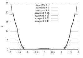
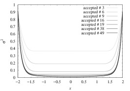
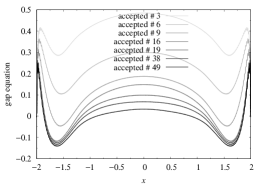
Figure 9: Initial stage of the random walk: the algorithm tries to reduce the numerical error the most by bringing down $\sigma(0)$ towards zero.

Unfortunately, the randomly chosen (by the algorithm) values of $\lambda$ near the boundary yield too “sharp” a solution for $\sigma$; to mitigate this, the algorithm sees the numerical error can be reduced by “pushing out” the corners of $\lambda$ and adjusting the midpoint, $\lambda(0)$, which after enough cycles yields a solution for $\sigma$ to the gap equation and hence a solution for $\lambda$, see Fig. 10. The algorithm terminates when the error is below a given acceptable threshold (errtol). The solution is shown as a black line in Fig. 10; i.e. this solution has been accepted with an error tolerance of errtol $=6\times 10^{-5}$.

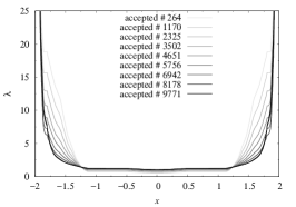
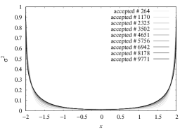
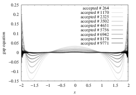
Figure 10: Later stage of the random walk: the algorithm reduces the numerical error by “pushing out” the corners of $\lambda$ and adjusting $\lambda(0)$.

Finally, in Fig. 11 we display the midpoint values of $\lambda$ and $\sigma^{2}$ as functions of acceptance numbers (which roughly corresponds to running time of the numerical calculation).

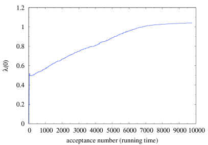
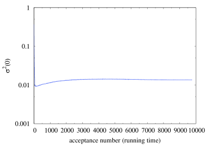
Figure 11: The value of $\lambda$ and $\sigma$ at the midpoint of the string as functions of acceptance number (running time).

References

- [1] A. D’Adda, M. Luscher and P. Di Vecchia, “A 1/n Expandable Series of Nonlinear Sigma Models with Instantons,” Nucl. Phys. B 146 (1978) 63.
- [2] E. Witten, “Instantons, the Quark Model, and the 1/n Expansion,” Nucl. Phys. B 149 (1979) 285.
- [3] S. Bolognesi, K. Konishi and K. Ohashi, “Large- sigma model on a finite interval,” JHEP 1610, 073 (2016) doi:10.1007 [arXiv:1604.05630 [hep-th]].
- [4] R. Auzzi, S. Bolognesi, J. Evslin and K. Konishi, “NonAbelian monopoles and the vortices that confine them,” Nucl. Phys. B 686 (2004) 119 [hep-th/0312233];
- [5] K. Konishi, A. Michelini and K. Ohashi, “Monopole-vortex complex in a theta vacuum,” Phys. Rev. D 82, 125028 (2010) [arXiv:1009.2042 [hep-th]];
- [6] M. Cipriani, D. Dorigoni, S. B. Gudnason, K. Konishi and A. Michelini, “Non-Abelian monopole-vortex complex,” Phys. Rev. D 84, 045024 (2011) [arXiv:1106.4214 [hep-th]];
- [7] C. Chatterjee and K. Konishi, “Monopole-vortex complex at large distances and nonAbelian duality,” JHEP 1409, 039 (2014) [arXiv:1406.5639 [hep-th]].
- [8] A. Hanany and D. Tong, “Vortices, instantons and branes,” JHEP 0307 (2003) 037 [hep-th/0306150].
- [9] L. Auzzi, S. Bolognesi, J. Evslin, K. Konishi and A. Yung, “NonAbelian superconductors: Vortices and confinement in N=2 SQCD,” Nucl. Phys. B 673 (2003) 187 [hep-th/0307287].
- [10] M. Shifman and A. Yung, “NonAbelian string junctions as confined monopoles,” Phys. Rev. D 70, 045004 (2004) [hep-th/0403149].
- [11] A. Milekhin, “CP(N-1) model on finite interval in the large N limit,” Phys. Lev. D 86 (2012) 105002 [arXiv:1207.0417 [hep-th]].
- [12] S. Monin, M. Shifman and A. Yung, “Non-Abelian String of a Finite Length,” Phys. Rev. D 92 (2015) no.2, 025011 [arXiv:1505.07797 [hep-th]].
- [13] A. Milekhin, “CP(N) sigma model on a finite interval revisited,” Phys. Rev. D 95 (2017) no.8, 085021 doi:10.1103/PhysRevD.95.085021 [arXiv:1612.02075 [hep-th]].
- [14] A. Actor, “Temperature Dependence Of The Cp**(n-1) Model And The Analogy With Quantum Chromodynamics,” Fortsch. Phys. 33 (1985) 333.
- [15] A. Flachi, M. Nitta, S. Takada and R. Yoshii, “Sign Flip in the Casimir Force for Interacting Fermion Systems,” Phys. Rev. Lett. 119 (2017) no.3, 031601 doi:10.1103/PhysRevLett.119.031601 [arXiv:1704.04918 [hep-th]].
- [16] M. Nitta and R. Yoshii, “Self-Consistent Exact Solutions of Inhomogneous Condensates in Quantum Model,” arXiv:1707.03207 [hep-th].
- [17] A. Flachi, M. Nitta, S. Takada and R. Yoshii, “Casimir Force for the Model,” arXiv:1708.08807 [hep-th].
- [18] D. Pavshinkin, “Grassmannian sigma model on a finite interval,” arXiv:1708.06399 [hep-th].