Magnetic field generation by pointwise zero-helicity three-dimensional steady flow of incompressible electrically conducting fluid

Abstract

We introduce six families of three-dimensional space-periodic steady solenoidal flows, whose kinetic helicity density is zero at any point. Four families are analytically defined. Flows in four families have zero helicity spectrum. Sample flows from five families are used to demonstrate numerically that neither zero kinetic helicity density, nor zero helicity spectrum prohibit generation of large-scale magnetic field by the two most prominent dynamo mechanisms: the magnetic $\alpha$-effect and negative eddy diffusivity. Our computations also attest that such flows often generate small-scale field for sufficiently small magnetic molecular diffusivity. These findings indicate that kinetic helicity and helicity spectrum are not the quantities controlling the dynamo properties of a flow regardless of whether scale separation is present or not.

1 Introduction

Consider a volume $\Omega$ transported by an ideal incompressible fluid flow $\bf v$, such that initially the vorticity $\nabla\times\bf v$ is tangent to the boundary $\partial\Omega$. Since the vorticity lines are frozen in the fluid, the vorticity remains tangent to $\partial\Omega$ at all times, and the value

$$\int_{\Omega}{\bf v}\cdot(\nabla\times{\bf v})\,{\rm d}{\bf x},$$

called kinetic helicity, does not change in time. This was shown for barotropic gas in Mor and independently (see Mof and https://sites.google.com/site/hkeithmoffatt/selected-publications-1960s) in M69 (see also KhCh ; MT ; AK ). In space-periodic flows, the total kinetic helicity in a periodicity cell is also conserved. Recent measurements of the total helicity of vortex tubes in water demonstrated that even in viscous fluid the total helicity can remain constant or saturate to a constant (or almost constant) value SRK .

In a general setup, helicity $\cal H$ of a solenoidal vector field transported by a flow as a frozen field (e.g., a magnetic field or the flow vorticity) is defined as the volume-integrated scalar product of the field and its vector potential (by this definition, the kinetic helicity is the vorticity helicity). Following MR , consider a tube carrying flux $\Phi$ and consisting of closed field lines that have no inflexion points (i.e., whose curvature does not vanish at any point). It can be proven that for such a tube

$${\cal H}=n\Phi^{2},$$ (1)

where $n$ is a conserved quantity. This invariant quantifies a fundamental topological property of the field, the knottedness of its field lines. If the tube under consideration is unknotted, but any pair of field lines in it is linked, the linking number, $\cal N$, being the same for each pair, then $n=\cal N$. In general, $n={\cal W}+{\cal T}+{\cal N}$, where the writhe, $\cal W$, and the normalised total torsion of a center field-line, $\cal T$, characterise how the tube itself is knotted (see an intuitive illustration of these concepts in Figs. 7 and 12 of MR ).

Containing important information about the topological structure of the flow, helicity plays a significant role in physics (see the references in KFDI ). In geophysical or astrophysical contexts, as well as in laboratory experiments, flows are often accompanied by rotation and consequently they are usually helical. Helicity arises in convection LB ; Ge and turbulence PM . Participation of helicity in generation of a dipolar magnetic field in a geodynamo model involving convection in a rapidly rotating spherical shell was explored in SJ . Generation of cosmic magnetic fields of the intensity and spatial scale that is observed in astrophysics is believed to be possible due to the chirality of the background turbulence characterised by a non-zero kinetic helicity Mof . Moreover, apparently the dynamo action of a flow is guaranteed if the mean helicity is of constant sign over a sufficiently large extent of fluid Mof .

Investigating the electromotive force (e.m.f.) due to the interaction of small-scale fluctuations of the flow and magnetic field is a pillar of the magnetic dynamo theory. The small-scale e.m.f. may have a non-zero mean component parallel to the mean magnetic field, and this is often beneficial for magnetic field generation. This seminal idea goes back to E. Parker P55 , who called such fluctuations of the flow “cyclonic events”. The part of the mean e.m.f. linear in the mean field gives rise to the so-called magnetic $\alpha$-effect. A systematic treatment of this idea under various simplifying assumptions is the topic of mean-field electrodynamics SKR ; KR .

Clearly, an intricate spatial structure of the small-scale fluctuating component of a flow (and hence, by virtue of the induction equation, of the magnetic field) is expected to correlate with a high degree of the vorticity knottedness and — since this hydrodynamic invariant constrains the topology of vorticity lines — with a non-zero kinetic helicity. Thus, kinetic helicity may be intimately related with magnetic field generation — for instance, it may control the strength of the magnetic $\alpha$-effect. Some observations confirm this conjecture: On the one hand, the $\alpha$-effect coefficient was calculated in the second-order correlation approximation and high-conductivity limit for the isotropic turbulence (see, e.g., KHR ), and it turned out to be proportional to the mean kinetic helicity. This result was also derived in M74 in the limit of ideal magnetohydrodynamics for rotationally symmetric turbulence with the use of Lagrangian coordinates for description of the evolution of the field. On the other, by the Zeldovich Zel antidynamo theorem, a two-dimensional flow of incompressible fluid cannot generate magnetic field — and its mean kinetic helicity is zero if the flow is space-periodic or satisfies some other suitable boundary conditions; moreover, it is pointwise non-helical,

$${\bf v}\cdot(\nabla\times{\bf v})=0,$$ (2)

when it does not depend on the coordinate in the direction perpendicular to the parallel planes, to which the fluid motion is confined.

However, it became clear decades ago that the mean helicity is unnecessary for the dynamo action of smooth (laminar) flows, see, e.g., GFP ; RBr . More specifically, a non-zero kinetic helicity is required neither for generation of small-scale (i.e., having the same spatial periods as the flow velocity) magnetic field, nor for creating the $\alpha$-effect for generation of the large-scale magnetic field. Not much helicity is needed to drive large-scale nonlinear dynamos GBMP . Nevertheless, parallels between the generation in various magnetohydrodynamic (MHD) setups and a non-zero kinetic helicity of the generating flow are often drawn in the literature. The following argument is often encountered: the $\alpha$-effect requires the lack of reflectional symmetry in the flow, and for physicist kinetic helicity is the simplest measure of this (since the helicity vanishes for parity-invariant and mirror-symmetric flows). This point of view is amenable to the following criticism: first, many other functionals, such as the flow helicity (or the helicity of any real power of the Laplacian of the flow or vorticity) have the same property; and, second, the total kinetic helicity also vanishes for flows that are parity-antiinvariant or have reflectional antisymmetry. Similarly, helicity spectrum vanishes not only for parity-invariant flows, but also for parity-antiinvariant ones (see section 3.6).

The discussion above implies that exploring the dynamics of ideal fluid flow or evolution of magnetic field (note that formally vorticity satisfies the same equation as the magnetic field) transported by flows of complex topology may require constructing flows with a desirable knot structure of field lines. A systematic procedure for constructing solenoidal vector fields with tunable helicity, whose closed field lines involve knots of many types, was presented in KFDI . It relies on a method for calculating vector potentials of the fields that employs complex scalar functions. Examples of knotted fields were presented, whose mean helicity is zero.

We focus on the study of the kinematic dynamo action of steady three-dimensional flows of incompressible fluid and demand that the flow ultimately lacks kinetic helicity, the flow and vorticity being orthogonal at each point (2); we will call such flows non-helical. In section 3 we present six families of steady solenoidal pointwise non-helical flows. By necessity, our approach is constructive: flows from four families are analytically defined, from another one can be obtained by semianalytical procedures. Sample flows belonging to each of the five families are used to study kinematic dynamos. Four families out of the five are composed of flows, whose helicity spectrum is zero; we therefore simultaneously verify that a non-zero helicity spectrum is unnecessary for generation of large- or small-scale flows.

Let us mention the small-scale kinematic dynamo ZG powered by the Christopherson flow Chr :

$${\bf v}=\left({L^{2}\over 4\pi}{\partial g\over\partial x_{1}}\cos\pi x_{3},\quad{L^{2}\over 4\pi}{\partial g\over\partial x_{2}}\cos\pi x_{3},\quad{g\over 3}\sin\pi x_{3}\right),$$ (3)

where

$$g(x_{1},x_{2})=\cos{2\pi x_{1}\over\sqrt{3}L}+2\cos{\pi x_{1}\over\sqrt{3}L}\cos{\pi x_{2}\over L}.$$

It satisfies (2) and nevertheless generates magnetic field when the magnetic Reynolds number exceeds the critical value $R_{m}\approx 515.63$ ZG . Matthews Mat questioned whether the resolution in computations ZG was sufficient. We have now repeated the computations with the double resolution of $128^{3}$ poloidal and $128^{3}$ toroidal modes, and recovered the magnetic field growth rates of ZG , increasing from -0.000377 for $R_{m}=500$ to 0.006786 for $R_{m}=1000$, with an accuracy better than $10^{-6}$, this confirming the results of ZG . The energy spectrum of the dominant magnetic eigenmodes falls off by at least 11 orders of magnitude indicating that the resolution that we have now used is exceedingly high. The estimate $R_{m}=515.63$ for the critical value was obtained in ZG by linear interpolation of growth rates between the two neighbour integer magnetic Reynolds numbers; the present double resolution computations yield for this $R_{m}$ the growth rate $1.2\times 10^{-5}$.

Many examples of dynamos can be found in the literature, in which the total kinetic helicity vanishes. However, to the best of our knowledge, the Christopherson flow is the only documented example of a three-dimensional steady flow of incompressible fluid, whose helicity density is zero at each point in space (2), and which is capable of dynamo action. This example is unsatisfactory in that it is a dynamo only for specific boundary conditions (see Mat ). We consider only space-periodic flows and magnetic fields in order to exclude the influence of boundaries, the flow periodicity cell being a cube ${\mathbb{T}}^{3}=[0,2\pi]^{3}$. Our goal is to demonstrate that it is typical for a pointwise non-helical steady flow to generate magnetic field for a sufficiently small magnetic molecular diffusivity, regardless of whether scale separation is present or not. In particular, we will show that such flows typically can power the two most prominent mechanisms for generation of large-scale fields: the magnetic $\alpha$-effect when the flow lacks parity invariance, or negative magnetic eddy diffusivity otherwise. It turns out that many of these flows can also act as small-scale kinematic dynamos.

The paper is organised as follows. We present large-scale kinematic dynamos based on the magnetic $\alpha$-effect in section 4, and negative magnetic eddy diffusivity in section 5. We need a sufficient stock of non-helical flows for numerical experimentation, and in section 3 we discuss semianalytical techniques for constructing them, as well as present analytical examples of such flows. In a multiscale setup, the magnetic $\alpha$-effect and eddy diffusivity tensors have been calculated by asymptotic methods (see, e.g., chapter 3 of VZ ). Our approach relies on this analysis and, for the reader’s convenience, in the next section we summarise and enhance it tailoring to the needs of the present investigation. The notion of the helicity spectrum arises naturally in the theory of the magnetic $\alpha$-effect in MHD turbulence M70 ; MP ; we briefly discuss in section 2.3 its relevance when the local magnetic Reynolds number is small and evaluate in section 3.6 the helicity spectrum of the flows that we use in computations.

2 The magnetic $\alpha$-effect and eddy diffusivity

We review here the multiscale formalism arising in the study of the kinematic generation of large-scale magnetic field by a small-scale zero-mean steady flow $\bf v$ of conducting fluid (see VZ for a more detailed discussion and a comprehensive list of references). In this section no assumptions about the kinetic helicity are made.

In mathematical terms, we consider the eigenvalue problem for the magnetic induction operator

$$\L{\bf b}\equiv\eta\nabla^{2}{\bf b}+\nabla\times({\bf v}\times{\bf b})=\lambda{\bf b}.$$ (4)

Here $\eta$ is the magnetic molecular diffusivity, $\bf b$ a magnetic mode and Re $\lambda$ its growth rate (a negative growth rate actually indicates that a mode is decaying). The mode is solenoidal,

$$\nabla\cdot{\bf b}=0,$$ (5)

and the fluid is supposed to be incompressible, $\nabla\cdot{\bf v}=0$.

The two-scale nature of the magnetic mode $\bf b$ is reflected by its dependence on the so-called fast, $\bf x$, and slow, ${\bf X}=\varepsilon\bf x$, spatial variables; by contrast, the small-scale flow $\bf v$ depends only on $\bf x$. The scale ratio $\varepsilon$ is assumed to be small, which enables us to apply asymptotic methods. (The difference in approaches is notable: while we consider the limit $\varepsilon\to 0$ only, the theory of mean-field electrodynamics strives to estimate the impact of all small and intermediate scales on the large-scale magnetic field, somewhat in the spirit of the LES closures; see ABNZ .) One proceeds by substituting power series expansions

$${\bf b} =\sum_{n=0}^{\infty}{\bf b}_{n}({\bf X},{\bf x})\,\varepsilon^{n},$$ (.1)

$$\lambda =\sum_{n=0}^{\infty}\lambda_{n}\varepsilon^{n}$$ (.2)

into (4) and (5), and deriving a hierarchy of equations emerging at successive orders $\varepsilon^{n}$.

2.1 Magnetic $\alpha$-effect

The relevant solution to the first (order $\varepsilon^{0}$) equation in the hierarchy is

$${\bf b}_{0}=\sum_{k=1}^{3}\left\langle{\bf b}_{0}\right\rangle_{k}({\bf e}_{k}+{\bf S}_{k}),\qquad\lambda_{0}=0,$$

where

$$\left\langle{\bf f}\right\rangle=(2\pi)^{-3}\int_{{\mathbb{T}}^{3}}{\bf f}({\bf X},{\bf x})\,{\rm d}{\bf x}=\sum_{k=1}^{3}\left\langle{\bf f}\right\rangle_{k}{\bf e}_{k}$$

denotes the mean over the periodicity cell ${\mathbb{T}}^{3}$ in the fast variables (i.e., over small scales; note that no other means are appropriate), ${\bf e}_{k}$ are unit vectors of the Cartesian coordinate system and ${\bf S}_{k}({\bf x})$ are zero-mean small-scale solenoidal solutions to 3 auxiliary problems of type I:

$$\L{\bf S}_{k}=-{\partial{\bf v}\over\partial x_{k}}\qquad\Leftrightarrow\qquad\L({\bf S}_{k}+{\bf e}_{k})=0$$ (7)

(the magnetic induction operator $\L$ is henceforth assumed to involve differentiation in fast variables $\bf x$ only; we will call it the large-scale magnetic induction operator when full differentiation in space is performed). It is easy to show that such solutions exist, see, e.g., section 3.2 of VZ .

The solvability condition for the second (order $\varepsilon^{1}$) equation in the hierarchy is an eigenvalue problem,

$$\nabla_{\bf X}\times(\boldsymbol{\mathfrak{A}}\left\langle{\bf b}_{0}\right\rangle)=\lambda_{1}\left\langle{\bf b}_{0}\right\rangle,\qquad\nabla_{\bf X}\cdot\left\langle{\bf b}_{0}\right\rangle=0,$$ (8)

(the subscript $\bf X$ marks differential operators in slow variables) from which we determine $\lambda_{1}$ and, generically, $\left\langle{\bf b}_{0}\right\rangle$. Here $\boldsymbol{\mathfrak{A}}$ is the so-called tensor of the magnetic $\alpha$-effect, a $3\times 3$ matrix, whose $k$th column is

$$\boldsymbol{\mathfrak{A}}_{k}=\left\langle{\bf v}\times{\bf S}_{k}\right\rangle.$$ (9)

This expression is consistent with the original Parker’s idea that the interaction of fine structures of a flow (in our case, $\bf v$) and magnetic field ($\sum_{k=1}^{3}\left\langle{\bf b}_{0}\right\rangle_{k}{\bf S}_{k}$) gives rise to a mean e.m.f. ($\boldsymbol{\mathfrak{A}}\left\langle{\bf b}_{0}\right\rangle$) that may have a component, parallel to the large-scale magnetic field ($\left\langle{\bf b}_{0}\right\rangle$, respectively).

To solve the eigenvalue problem (8), we assume that the mean field is a Fourier harmonics,

$$\left\langle{\bf b}_{0}\right\rangle={\bf B}{\rm e}^{{\rm i}\bf q\cdot X}.$$ (10)

Here $\bf q$ and $\bf B$ are constant vectors, $|{\bf q}|=1$. It is convenient to express the wave vector in spherical coordinates, whose axis is aligned with the Cartesian axis $x_{3}$ (the assumed vertical direction):

$$q_{1}=\sin\theta\,\cos\varphi,\qquad q_{2}=\sin\theta\,\sin\varphi,\qquad q_{3}=\cos\theta.$$ (.1)

Since the solenoidality of $$\left\langle{\bf b}_{0}\right\rangle {\bf B\cdot q}=0$$ translates into the orthogonality , we can expand

$${\bf B}=B_{t}{\bf q}^{\rm t}+B_{p}{\bf q}^{\rm p},$$ (.2)

where unit vectors

$${\bf q}^{\rm p}=(\cos\theta\,\cos\varphi,\,\cos\theta\,\sin\varphi,\,-\sin\theta),\qquad{\bf q}^{\rm t}=(-\sin\varphi,\cos\varphi,0)$$ (.3)

constitute, together with $\bf q$, an orthonormal basis of positive orientation in ${\mathbb{R}}^{3}$. This reduces (8) to an eigenvalue problem for a $2\times 2$ matrix:

$${\rm i}\left[\begin{array}[]{rr}{\bf q}^{\rm p}\cdot\boldsymbol{\mathfrak{A}}{\bf q}^{\rm t}&{\bf q}^{\rm p}\cdot\boldsymbol{\mathfrak{A}}{\bf q}^{\rm p}\\ -{\bf q}^{\rm t}\cdot\boldsymbol{\mathfrak{A}}{\bf q}^{\rm t}&-{\bf q}^{\rm t}\cdot\boldsymbol{\mathfrak{A}}{\bf q}^{\rm p}\end{array}\right]\left[\begin{array}[]{l}B_{t}\\ B_{p}\end{array}\right]=\lambda_{1}({\bf q})\left[\begin{array}[]{l}B_{t}\\ B_{p}\end{array}\right].$$ (12)

The eigenvalues are now obtained by straightforward algebra (the identity $q^{\rm p}_{n}q^{\rm t}_{n^{\prime}}-q^{\rm t}_{n}q^{\rm p}_{n^{\prime}}=\epsilon_{jnn^{\prime}}q_{j}$ is useful, where $\epsilon_{jln}$ is the unit antisymmetric tensor). In terms of wave vector components they are

$$\lambda_{1_{\pm}}({\bf q})= \,{{\rm i}\over 2}\left((\mathfrak{A}^{2}_{3}-\mathfrak{A}^{3}_{2})q_{1}+(\mathfrak{A}^{3}_{1}-\mathfrak{A}^{1}_{3})q_{2}+(\mathfrak{A}^{1}_{2}-\mathfrak{A}^{2}_{1})q_{3}\vphantom{{}^{2}}\right)\pm\sqrt{a},$$ (.1)

$$a= \,(\mathfrak{A}_{2}^{2}\mathfrak{A}_{3}^{3}-({{}^{\rm s}\mathfrak{A}}^{2}_{3})^{2})q_{1}^{2}+(\mathfrak{A}_{1}^{1}\mathfrak{A}_{3}^{3}-({{}^{\rm s}\mathfrak{A}}^{1}_{3})^{2})q_{2}^{2}+(\mathfrak{A}_{1}^{1}\mathfrak{A}_{2}^{2}-({{}^{\rm s}\mathfrak{A}}^{1}_{2})^{2})q_{3}^{2}$$ (.2)

$$+2\left(({{}^{\rm s}\mathfrak{A}}^{1}_{2}{{}^{\rm s}\mathfrak{A}}^{1}_{3}-{{}^{\rm s}\mathfrak{A}}^{2}_{3}\mathfrak{A}_{1}^{1})q_{2}q_{3}\vphantom{{}^{2}}+({{}^{\rm s}\mathfrak{A}}^{1}_{2}{{}^{\rm s}\mathfrak{A}}^{2}_{3}-{{}^{\rm s}\mathfrak{A}}^{1}_{3}\mathfrak{A}_{2}^{2})q_{1}q_{3}+({{}^{\rm s}\mathfrak{A}}^{1}_{3}{{}^{\rm s}\mathfrak{A}}^{2}_{3}-{{}^{\rm s}\mathfrak{A}}^{1}_{2}\mathfrak{A}_{3}^{3})q_{1}q_{2}\right),$$

where ${{}^{\rm s}\mathfrak{A}}_{i}^{j}=(\mathfrak{A}_{i}^{j}+\mathfrak{A}_{j}^{i})/2$ are entries of the symmetrised $\alpha$-tensor ${{}^{\rm s}\boldsymbol{\mathfrak{A}}}=(\boldsymbol{\mathfrak{A}}+\boldsymbol{\mathfrak{A}}^{*})/2$. Comparison of (.2) with the formula for ${{}^{\rm s}\boldsymbol{\mathfrak{A}}}^{-1}$ (provided ${{}^{\rm s}\boldsymbol{\mathfrak{A}}}$ is invertible) in terms of cofactors (see, e.g., Shi ) reveals a compact expression

$$a={\bf q}\cdot(\det{{}^{\rm s}\boldsymbol{\mathfrak{A}}})\,{{}^{\rm s}\boldsymbol{\mathfrak{A}}}^{-1}\bf q.$$

For $a\leq 0$, the $\alpha$-effect just sustains constant-amplitude oscillations of a mean magnetic mode (10) in the slow time $T_{1}=\varepsilon t$. Consider now wave vectors $\bf q$ for which $a>0$. By virtue of (.1), the slow-time growth rate Re$\,\lambda_{1_{+}}({\bf q})=\sqrt{a}$ of the large-scale magnetic field depends only on the entries of the symmetric matrix ${{}^{\rm s}\boldsymbol{\mathfrak{A}}}$. This helps to determine the maximum growth rate Re$\,\lambda_{1}({\bf q})$ over unit wave vectors: Eigenvalues $\alpha_{i}$ of ${{}^{\rm s}\boldsymbol{\mathfrak{A}}}$ are real and the associated eigenvectors are mutually orthogonal. The relation (.2) remains applicable in the Cartesian coordinate system, whose axes coincide with eigendirections of ${{}^{\rm s}\boldsymbol{\mathfrak{A}}}$; thus

$$a=\alpha_{1}\alpha_{2}(q^{\prime}_{3})^{2}+\alpha_{2}\alpha_{3}(q^{\prime}_{1})^{2}+\alpha_{1}\alpha_{3}(q^{\prime}_{2})^{2},$$

where $q^{\prime}_{i}$ are components of $\bf q$ in the basis of the eigenvectors of ${{}^{\rm s}\boldsymbol{\mathfrak{A}}}$ (cf. section 9.3 of Mb ). Denoting the maximum slow-time growth rate due to the action of the $\alpha$-effect by $\gamma_{\alpha}$, we find

$$\gamma_{\alpha}\equiv\max_{|{\bf q}|=1}{\rm Re}\,\lambda_{1_{\pm}}({\bf q})=\sqrt{\max(\alpha_{1}\alpha_{2},\,\alpha_{2}\alpha_{3},\,\alpha_{1}\alpha_{3})}.$$ (14)

A few comments stemming from (13) are in order.

$i$. The spectrum of the $\alpha$-effect operator, ${\bf b(X)}\mapsto\nabla_{\bf X}\times(\boldsymbol{\mathfrak{A}}{\bf b})$, is symmetric about the real and imaginary axes. Generically, $\boldsymbol{\mathfrak{A}}$ is a non-symmetric matrix; thus, the temporal growth or decay of a mean magnetic mode is accompanied by oscillations in the slow time $T_{1}$, whose frequency is controlled by the antisymmetric part, $\boldsymbol{\mathfrak{A}}-{{}^{\rm s}\boldsymbol{\mathfrak{A}}}$, of the $\alpha$-tensor.

$ii$. The maximum slow-time growth rate (14) is strictly positive unless an eigenvalue of ${{}^{\rm s}\boldsymbol{\mathfrak{A}}}$ is zero, another one is non-negative, and the third one is non-positive. If all the three $\alpha_{i}$ have the same signs, then for each $\bf q$ there exist a growing and decaying mean magnetic mode. If two eigenvalues have the same sign and the third one has the opposite sign, then for some $\bf q$ both modes experience constant-amplitude oscillations in the slow time $T_{1}$. The wave vectors for which the modes exhibit such a purely oscillatory behaviour form a cone, whose cross-section is elliptic and whose axis is aligned with the eigenvector associated with the third eigenvalue.

$iii$. When $\boldsymbol{\mathfrak{A}}$ is the identity matrix, $\lambda_{1_{\pm}}({\bf q})=\pm 1$ for all unit wave vectors. In particular, the proper subspace associated with the eigenvalue 1 for ${\bf q}=\pm{\bf e}_{i}$ is six-fold. ABC-flows Arn and their spatial derivatives constitute a basis in it.

Provided the eigenvalues (13) are distinct (i.e., $a\neq 0$) and the magnetic induction operator $\L$ does not have zero-mean neutral modes (generically the two conditions hold true), all terms in the series (6) can be determined from the hierarchy of equations obtained by substituting the series into (4) and (5). It was proven in V87 that if the symmetrised tensor ${{}^{\rm s}\boldsymbol{\mathfrak{A}}}$ is positively or negatively defined (and if the spatial periodicity of the eigenfunction is compatible with that of the flow), then the series (6), constructed for any solution (10), (13) to the eigenvalue problem (8) for the $\alpha$-effect operator, converge for sufficiently small $\varepsilon$ in suitable Sobolev spaces; the sums are analytical in $\varepsilon$ functions that solve the eigenvalue problem for the large-scale magnetic induction operator. In other words, a unique $\varepsilon$-parameterised branch of the eigenvalues (.2) of the large-scale magnetic induction operator originates from any simple eigenvalue $\lambda_{1}$ of the $\alpha$-effect operator.

“Uncurling” (7), we find

$$-\eta\,\nabla\times{\bf S}_{k}+{\bf v}\times({\bf S}_{k}+{\bf e}_{k})=\left\langle{\bf v}\times{\bf S}_{k}\right\rangle+\nabla p_{k},$$ (15)

where $p_{k}({\bf x})$ are space-periodic functions. This identity was used in VZ (see p. 34) to demonstrate that the $\alpha$-effect is linked with the helicity of the current density $\nabla\times{\bf S}_{k}$: scalar multiplying (15) by ${\bf S}_{l}+{\bf e}_{l}$ and averaging the result over the periodicity cell yields

$$-\eta\,\left\langle{\bf S}_{l}\cdot\nabla\times{\bf S}_{k}\right\rangle+\left\langle({\bf S}_{l}+{\bf e}_{l})\cdot({\bf v}\times({\bf S}_{k}+{\bf e}_{k}))\right\rangle=\mathfrak{A}^{l}_{k},$$

whereby

$$-2\eta\,\left\langle{\bf S}_{l}\cdot\nabla\times{\bf S}_{k}\right\rangle=\mathfrak{A}^{l}_{k}+\mathfrak{A}^{k}_{l};$$ (.1)

for $$k=l$$ this relation reduces to

$$-\eta\,\left\langle{\bf S}_{k}\cdot\nabla\times{\bf S}_{k}\right\rangle=\mathfrak{A}_{k}^{k}.$$ (.2)

The identity (15) also implies a relation between the tensors $\boldsymbol{\mathfrak{A}}$ and $\boldsymbol{\mathfrak{A}}^{-}$ of the magnetic $\alpha$-effect for a flow $\bf v$ and the reverse flow $-\bf v$, respectively. Let us denote by $\L^{-}$ the magnetic induction operator for the reverse flow $-\bf v$,

$$\L^{-}{\bf b}=\eta\nabla^{2}{\bf b}-\nabla\times({\bf v}\times{\bf b})$$ (17)

(involving differentiation in the fast variables $\bf x$ only), whose kernel is spanned by the neutral modes ${\bf S}^{-}_{l}+{\bf e}_{l}$:

$$\L^{-}({\bf S}^{-}_{l}+{\bf e}_{l})=0,\qquad\left\langle{\bf S}^{-}_{l}\right\rangle=0.$$ (18)

This equation is equivalent to

$$-\eta\,\nabla\times{\bf S}^{-}_{l}-{\bf v}\times({\bf S}^{-}_{l}+{\bf e}_{l})=\left\langle-{\bf v}\times{\bf S}^{-}_{l}\right\rangle+\nabla p^{-}_{l}.$$ (19)

Scalar multiplying (15) by ${\bf S}^{-}_{l}+{\bf e}_{l}$ and averaging the result over the periodicity cell yields

$$-\eta\,\left\langle{\bf S}^{-}_{l}\cdot\nabla\times{\bf S}_{k}\right\rangle+\left\langle({\bf S}^{-}_{l}+{\bf e}_{l})\cdot({\bf v}\times({\bf S}_{k}+{\bf e}_{k}))\right\rangle=\mathfrak{A}^{l}_{k}.$$

Similarly, from (19)

$$-\eta\,\left\langle{\bf S}_{k}\cdot\nabla\times{\bf S}^{-}_{l}\right\rangle-\left\langle({\bf S}_{k}+{\bf e}_{k})\cdot({\bf v}\times({\bf S}^{-}_{l}+{\bf e}_{l}))\right\rangle=(\mathfrak{A}^{-})^{k}_{l}.$$

By comparison of the above relations, $(\mathfrak{A}^{-})^{k}_{l}=\mathfrak{A}^{l}_{k}$, i.e., the $\alpha$-effect tensor $\boldsymbol{\mathfrak{A}}^{-}$ for the reverse flow $-\bf v$ is obtained from the tensor $\boldsymbol{\mathfrak{A}}$ for $\bf v$ by transposition. Consequently, the maximum slow-time growth rates due to the action of the $\alpha$-effect in the direct and reverse flows coincide.

2.2 Magnetic eddy diffusivity

An important non-generic case is that of the absence of the $\alpha$-effect, i.e., when $\boldsymbol{\mathfrak{A}}=0$, whereby (8) yields $\lambda_{1}=0$, but $\left\langle{\bf b}_{0}\right\rangle$ remains undetermined. This occurs, e.g., if the flow $\bf v$ is parity-invariant (a vector field $\bf f$ is parity-invariant as long as ${\bf f}(-{\bf x})=-{\bf f}({\bf x})$ and parity-antiinvariant when ${\bf f}(-{\bf x})={\bf f}({\bf x})$). For such flows, parity-invariant and parity-antiinvariant fields constitute invariant subspaces of the magnetic induction operator (4). Consequently, ${\bf S}_{k}({\bf x})$ are parity-antiinvariant implying $\boldsymbol{\mathfrak{A}}=0$.

From the second equation in the hierarchy we then find

$${\bf b}_{1}=\sum_{k=1}^{3}\sum_{m=1}^{3}{\partial\left\langle{\bf b}_{0}\right\rangle_{k}\over\partial X_{m}}\,{\bf G}_{mk},$$

where an appropriate normalisation of the magnetic mode $\bf b$ (.1) is assumed, and the small-scale zero-mean (not necessarily solenoidal!) fields ${\bf G}_{mk}({\bf x})$ are solutions to 9 auxiliary problems of type II:

$$\L{\bf G}_{mk}=-2\eta{\partial{\bf S}_{k}\over\partial x_{m}}-{\bf e}_{m}\times({\bf v}\times({\bf S}_{k}+{\bf e}_{k})).$$ (20)

When $\bf v$ is parity-invariant, ${\bf G}_{mk}({\bf x})$ are parity-invariant as well. (Actually, for such $\bf v$ no odd powers of $\varepsilon$ enter the series (.2) for the eigenvalue $\lambda$, and in the expansion (.1) of the mode, ${\bf b}_{n}$ are parity-antiinvariant for all even indices and parity-invariant for odd $n$, see section 3.5 of VZ .)

The mean magnetic mode $\left\langle{\bf b}_{0}\right\rangle$ is a solution to the eigenvalue problem for the operator of magnetic eddy diffusivity:

$$\eta\nabla^{2}_{\bf X}\left\langle{\bf b}_{0}\right\rangle+\nabla_{\bf X}\times\sum_{k=1}^{3}\sum_{m=1}^{3}\boldsymbol{\mathfrak{D}}_{mk}{\partial\left\langle{\bf b}_{0}\right\rangle_{k}\over\partial X_{m}}=\lambda_{2}\left\langle{\bf b}_{0}\right\rangle,$$ (21)

which is the solvability condition for the third (order $\varepsilon^{2}$) equation in the hierarchy. Here

$$\boldsymbol{\mathfrak{D}}_{mk}=\left\langle{\bf v}\times{\bf G}_{mk}\right\rangle$$ (22)

is the so-called tensor of magnetic eddy diffusivity correction. The expression (22) conveys the physically important idea that, like the $\alpha$-effect, eddy diffusivity is a manifestation of the interaction of fine structures of the flow and magnetic field, but due to the parity it is order $\varepsilon$ weaker than the $\alpha$-effect that is generically present in the absence of symmetries.

We solve (21) for the mean mode (10), following essentially the same approach (see ABNZ ) as is used in section 2.1 for the problem (8). Using the relations (11), we recast (21) into an eigenvalue problem for a $2\times 2$ matrix:

$$-\sum_{m,l,n}\mathfrak{D}^{l}_{mn}q^{\rm p}_{l}(B_{t}q^{\rm t}_{n}+B_{p}q^{\rm p}_{n})q_{m} =(\eta+\lambda_{2})B_{t},$$

$$\sum_{m,l,n}\mathfrak{D}^{l}_{mn}q^{\rm t}_{l}(B_{t}q^{\rm t}_{n}+B_{p}q^{\rm p}_{n})q_{m} =(\eta+\lambda_{2})B_{p}.$$

Clearly, it transforms into (12) upon changing $\eta+\lambda_{2}\to\lambda_{1}$ and $\sum_{m}\mathfrak{D}^{l}_{mn}q_{m}\to-{\rm i}\mathfrak{A}^{l}_{n}$. We use this analogy to write down the solution:

$$\lambda_{2_{\pm}}({\bf q}) =-\eta-{1\over 2}\sum_{j,l,n}(D^{l}_{n}-D^{n}_{l})q_{j}\pm\sqrt{d},$$ (.1)

$$d =\sum_{j,l,n}\left((({{}^{\rm s}\!D}^{l}_{n})^{2}-{{}^{\rm s}\!D}^{l}_{l}\,{{}^{\rm s}\!D}^{n}_{n})q_{j}^{2}-2q_{j}q_{n}({{}^{\rm s}\!D}^{l}_{n}\,{{}^{\rm s}\!D}^{l}_{j}-{{}^{\rm s}\!D}^{l}_{l}\,{{}^{\rm s}\!D}^{n}_{j})\right),$$ (.2)

where both sums are over even permutations of indices 1, 2 and 3 (i.e., $$\epsilon_{jln}=1$$) and it is denoted

$$D^{l}_{n}=\sum_{m}\mathfrak{D}^{l}_{mn}q_{m},\qquad{{}^{\rm s}\!D}^{l}_{n}=(D^{l}_{n}+D^{n}_{l})/2.$$ (.3)

As for the $\alpha$-effect operator, a compact expression

$$d=-{\bf q}\cdot(\det{{}^{\rm s}\bf D})\,{{}^{\rm s}\bf D}^{-1}\bf q$$

follows from (.2) if the matrix ${{}^{\rm s}\bf D}$ is invertible; however, this expression does not help any more to determine the minimum

$$\eta_{\rm eddy}\equiv\min_{|{\bf q}|=1}(-{\rm Re}\,\lambda_{2_{\pm}}({\bf q}))$$ (24)

called the minimum magnetic eddy diffusivity, since by (.3) ${{}^{\rm s}\bf D}$ depends on $\bf q$. If $d<0$, the magnetic mode experiences oscillations in the slow time $T_{2}=\varepsilon^{2}t$; then, in view of (23), the frequency of oscillations is controlled by the symmetric part, ${}^{\rm s}\boldsymbol{\mathfrak{D}}$, of the eddy diffusivity tensor, whose entries are $(\mathfrak{D}^{l}_{mn}+\mathfrak{D}^{n}_{ml})/2$, and the slow-time growth or decay rate of the mode is controlled by the antisymmetric part, $\boldsymbol{\mathfrak{D}}-{{}^{\rm s}\boldsymbol{\mathfrak{D}}}$.

Computing the eddy diffusivity correction tensor applying (22) requires solving 12 auxiliary problems (3 of type I and 9 of type II), which is numerically inefficient. A preferable alternative is to rely on the identity

$$\mathfrak{D}^{l}_{mk}=\left\langle{\bf Z}_{l}\cdot\left(2\eta{\partial{\bf S}_{k}\over\partial x_{m}}+{\bf e}_{m}\times({\bf v}\times({\bf S}_{k}+{\bf e}_{k}))\right)\right\rangle$$ (25)

expressing the entries of the tensor in terms of the solutions ${\bf S}_{k}$ to the 3 auxiliary problems of type I and zero-mean solutions ${\bf Z}_{l}$ to 3 auxiliary problems for the adjoint operator:

$$\L^{*}{\bf Z}_{l}={\bf v}\times{\bf e}_{l}\qquad\Leftrightarrow\qquad\L^{-}(\nabla\times{\bf Z}_{l}+{\bf e}_{l})=0,$$ (26)

where

$$\L^{*}\,{\bf z}=\eta\nabla^{2}{\bf z}-{\bf v}\times(\nabla\times{\bf z})$$

is the operator adjoint to $\L$, and $\L^{-}$ is the magnetic induction operator (17) for the reverse flow $-\bf v$. Unlike (22), (25) does not offer any evident physical interpretation. By comparison of (7) and (26),

$$\nabla\times{\bf Z}_{l}={\bf S}^{-}_{l}\quad\Rightarrow\quad{\bf Z}_{l}=\eta^{-1}\nabla^{-2}({\bf v}\times({\bf S}^{-}_{l}+{\bf e}_{l})).$$ (27)

Here $\nabla^{-2}$ denotes the inverse Laplacian in the fast variables and ${\bf S}^{-}_{l}+{\bf e}_{l}$ is a neutral mode of $\L^{-}$, see (18). When the small-scale dynamo does not operate (i.e., all eigenvalues of $\L$ have non-positive real parts), the six fields ${\bf S}_{k}+{\bf e}_{k}$ and ${\bf S}^{-}_{l}+{\bf e}_{l}$ can be computed as the small-scale dominant eigenmodes of the magnetic induction operators $\L$ and $\L^{-}$, respectively; the same small-scale eigenvalue code (e.g., Zh ) solves all the 6 eigenproblems (with the flow reversed, $\bf v\to-v$, when computing ${\bf S}^{-}_{l}$).

2.3 Dynamo powered by “weak turbulence”

The two-scale dynamos considered in this section thus far are characterised by order 1 local magnetic Reynolds numbers R${}_{m}^{\rm loc}=\ell\left\langle|{\bf v}|^{2}\right\rangle^{1/2}\!\!/\eta$, given that the small-scale flow $\bf v$, the size of its periodicity box $\ell=2\pi$ and the molecular diffusivity $\eta$ are all assumed to be non-dimensional and independent of the scale ratio $\varepsilon$ (in computations reported in sections 4 and 5, the flow has been normalised and its r.m.s. velocity is 1). The $\alpha$-effect tensor for dynamos driven by turbulence was expressed in terms of the helicity spectrum M70 ; MP . We will now reproduce this result for small R${}_{m}^{\rm loc}$ (this modelling magnetic field generation by “weak turbulence”) by the multiscale asymptotic techniques. R${}_{m}^{\rm loc}$ becomes small when either the molecular eddy diffusivity is large, or when the amplitude of the flow is small. Let us inquire into the two cases.

In the former case we consider the repeated limit $\varepsilon\to 0$ and $\eta\to\infty$. The first limit, in $\varepsilon$, yields the asymptotic expansions (6); we just need to calculate the second one, in $\eta$. From (7), the neutral modes have the asymptotics

$${\bf S}_{k}=-\eta^{-1}\nabla^{-2}{\partial{\bf v}\over\partial x_{k}}+{\rm O}(\eta^{-2}),$$

and hence the $\alpha$-effect tensor is composed of the columns (9)

$$\boldsymbol{\mathfrak{A}}_{k}=-\eta^{-1}\left\langle{\bf v}\times\nabla^{-2}{\partial{\bf v}\over\partial x_{k}}\right\rangle+{\rm O}(\eta^{-2}).$$ (28)

In the latter case a time-periodic velocity $\varepsilon^{1/N}{\bf v(x},t)$ is assumed; we thereby relax till the end of the section the condition of steadiness of the flow, in order to obtain the expression for the $\alpha$-effect tensor derived in MP by the Test Field Method. (Note that the multiscale formalism discussed in the previous subsections has been generalised to encompass dynamos, periodic in the fast time, see chapter 4 in VZ ; the present work is concerned with steady flows only, because they give rise to significantly computationally less demanding auxiliary problems than in the time-periodic setup.) Here $N>1$ is an integer. Following V86 (see also GFP ), we solve the Floquet problem $(-\partial/\partial t+\L){\bf b}=\lambda\bf b$ for large-scale magnetic modes $\bf b$ of the same period $2\pi/\omega$ in the fast time $t$ as that of the flow. The modified expansions (6) now take the form

$${\bf b}({\bf X,x},t) =\sum_{n=0}^{\infty}{\bf b}_{n}({\bf X,x},t)\,\varepsilon^{n/N},$$ (.1)

$$\lambda =\sum_{n=0}^{\infty}\lambda_{n}\varepsilon^{n/N}.$$ (.2)

Substituting them into the eigenvalue equation yields a hierarchy of equations

$$-{\partial{\bf b}_{n}\over\partial t}+\eta\nabla^{2}{\bf b}_{n}+\nabla\times({\bf v}\times{\bf b}_{n-1})+2\eta(\nabla\cdot\nabla_{\bf X}){\bf b}_{n-N}+\nabla_{\bf X}\times({\bf v}\times{\bf b}_{n-N-1})+\eta\nabla^{2}_{\bf X}{\bf b}_{n-2N}=\sum_{m=0}^{n}\lambda_{n-m}{\bf b}_{m}$$ (30)

from which we can successively find all terms in the series (29). For a steady flow $\bf v$ and $N=2$, (29) determined by this procedure were proven V86 to be asymptotic series for a multiscale solution to the eigenvalue problem for the magnetic induction operator (provided the eigenvalue $\lambda_{4}$ of the limit operator in the l.h.s. of (.1) has multiplicity 1, and the spatial periodicity of the eigenfunction is compatible with that of the flow); the proof can be recast for time-periodic flows.

Averaging over the space-time periodicity cell (we will denote this average by double angle brackets, $\langle\!\langle\ \rangle\!\rangle$) order $\varepsilon^{n/N}$ equations for $n\leq N+1$, we find $\lambda_{n}=0$ for all such $n$, provided $\langle\!\langle{\bf b}_{0}\rangle\!\rangle$ does not vanish identically. The order $\varepsilon^{0}$ equation yields ${\bf b}_{0}={\bf b}_{0}({\bf X})$. The order $\varepsilon^{1/N}$ equation is then equivalent to

$${\bf b}_{1}=(\partial/\partial t-\eta\nabla^{2})^{-1}({\bf b}_{0}\cdot\nabla)\bf v,$$ (31)

where the inverse operator is calculated in the space of vector fields, $2\pi$-periodic in space and $2\pi/\omega$-periodic in the fast time, whose spatio-temporal mean vanishes. Consequently, the order $\varepsilon^{(N+2)/N}$ equation becomes upon averaging a closed eigenvalue equation in ${\bf b}_{0}$:

$$\eta\nabla^{2}_{\bf X}{\bf b}_{0}+\nabla_{\bf X}\times(\boldsymbol{\mathfrak{A}}{\bf b}_{0})= \,\lambda_{4}{\bf b}_{0}\phantom{\lambda_{N+2}}\mbox{for}~{}N=2;$$ (.1)

$$\nabla_{\bf X}\times(\boldsymbol{\mathfrak{A}}{\bf b}_{0})= \,\lambda_{N+2}{\bf b}_{0}\phantom{\lambda_{4}}\mbox{for}~{}N>2,$$ (.2)

where the $\alpha$-effect tensor consists of columns

$$\boldsymbol{\mathfrak{A}}_{k}=\left\langle\left\langle{\bf v}\times\left({\partial\over\partial t}-\eta\nabla^{2}\right)^{-1}{\partial{\bf v}\over\partial x_{k}}\right\rangle\right\rangle.$$ (33)

In the two cases under consideration, the limit R${}_{m}^{\rm loc}\to 0$ is approached along different paths in the parameter space; thus, it is no wonder that the equation (.1) for determining the leading terms in the series (29) differs from (8) and (.2). Nevertheless, the $\alpha$-effect tensors are the same! (For steady flow, (33) clearly reduces to (28); in fact, calculations for a time-periodic flow in the first case yield an expression identical to (33), up to an O($\eta^{-2}$) discrepancy.)

Following M70 ; MP , we expand the velocity in a Fourier series,

$${\bf v(x},t)=\sum_{{\bf p},p^{\prime}}\hat{\bf v}_{{\bf p},p^{\prime}}\,{\rm e}^{{\rm i}(p^{\prime}\omega t+\bf p\cdot x)}$$

and transform (33):

$$\boldsymbol{\mathfrak{A}}_{k}=\sum_{{\bf p},p^{\prime}}{{\rm i}p_{k}\over{\rm i}p^{\prime}\omega+\eta|{\bf p}|^{2}}\,(\overline{\hat{\bf v}}_{{\bf p},p^{\prime}}\times\hat{\bf v}_{{\bf p},p^{\prime}}).$$

Here summation is over all integer-component four-dimensional vectors $({\bf p},p^{\prime})\neq 0$ and the bar denotes complex conjugation. The contribution of two terms with opposite indices, ${\bf p},p^{\prime}$ and $-{\bf p},-p^{\prime}$, is real. Since both factors in the vector product in the r.h.s. are normal to $\bf p$, the product is parallel to $\bf p$, and hence finally

$$\boldsymbol{\mathfrak{A}}_{k}=-\sum_{{\bf p},p^{\prime}}{\eta p_{k}{\bf p}\over p^{\prime 2}\omega^{2}+\eta^{2}|{\bf p}|^{4}}H_{{\bf p},p^{\prime}}.$$

Here

$$H_{{\bf p},p^{\prime}}=\overline{\hat{\bf v}}_{{\bf p},p^{\prime}}\cdot({\rm i}{\bf p}\times\hat{\bf v}_{{\bf p},p^{\prime}}),$$ (34)

called the helicity spectrum of the flow $\bf v$, is the set of Fourier coefficients of the convolution integral ${\cal C}({\bf r},\tau)=\langle\!\langle{\bf v(x},t)\cdot(\nabla\times{\bf v(x+r},t+\tau))\rangle\!\rangle$. Evidently, ${\cal C}(0,0)$ is the mean kinetic helicity. This only link between kinetic helicity and the helicity spectrum is loose: in general, pointwise vanishing of the kinetic helicity density (2) neither requires, nor implies vanishing of the helicity spectrum. We observe that for R${}_{m}^{\rm loc}\to 0$ no $\alpha$-effect is present if $H_{\bf p}=0$ for all $p$.

Suppose now the flow is parity-invariant and thus $\boldsymbol{\mathfrak{A}}=0$. As above for the $\alpha$-effect tensor, we first consider the limit of small local magnetic Reynolds numbers realised as a repeated limit $\varepsilon\to 0$ and $\eta\to\infty$. The evolutionary versions of (7) and (20) imply

$${\bf S}_{k}={\partial{\bf u}\over\partial x_{k}}+{\rm O}(\eta^{-2}),\qquad{\bf G}_{mk}=2\eta\left({\partial\over\partial t}-\eta\nabla^{2}\right)^{-1}{\partial^{2}{\bf u}\over\partial x_{k}\partial x_{m}}+{\bf e}_{m}\times({\bf u}\times{\bf e}_{k})+{\rm O}(\eta^{-2}),$$

where

$${\bf u}=(\partial/\partial t-\eta\nabla^{2})^{-1}{\bf v}.$$ (35)

By (22), where spatio-temporal averaging is assumed as required for time-periodic fields,

$$\boldsymbol{\mathfrak{D}}^{l}_{mk}=\epsilon_{nlk}\sum_{({\bf p},p^{\prime})\neq 0}{\overline{\hat{v}}\vphantom{\bf v}_{{\bf p},p^{\prime}}^{n}\hat{v}_{{\bf p},p^{\prime}}^{m}\over{\rm i}p^{\prime}\omega+\eta|{\bf p}|^{2}}+{\rm O}(\eta^{-2}),$$

where $n=6-l-k$ for $l\neq k$. This eddy diffusivity tensor corresponds to the “symmetric part of $\beta_{iml}$” in MP . Since ${{}^{\rm s}\bf D}$ vanishes in the leading order, $\lambda_{2_{\pm}}({\bf q})$ (.1) coincide up to an O$(\eta^{-2})$ discrepancy:

$$\lambda_{2_{\pm}}({\bf q})=-\eta-\eta\sum_{({\bf p},p^{\prime})\neq 0}{|{\bf p}|^{2}|{\bf q}\cdot\hat{\bf v}_{{\bf p},p^{\prime}}|^{2}\over p^{\prime 2}\omega^{2}+\eta^{2}|{\bf p}|^{4}}+{\rm O}(\eta^{-2}).$$

Hence, in this case eddy correction of magnetic diffusivity is predominantly positively defined and only enhances molecular diffusivity. (This is reminiscent of passive scalar transport Bi .) The “antisymmetric part of $\beta_{iml}$” of MP linked with the helicity spectrum does not show up in the leading terms of the asymptotic expansion.

In the second case, the flow $\varepsilon^{1/N}{\bf v(x})$ again forces expanding large-scale magnetic modes and associated eigenvalues in the power series (29) in $\varepsilon^{1/N}$. All terms can be determined from the hierarchy (30). As in the presence of the $\alpha$-effect, ${\bf b}_{0}={\bf b}_{0}({\bf X})$ and ${\bf b}_{1}$ satisfies (31). For a parity-invariant flow, ${\bf b}_{n}$ are parity-antiinvariant for $n\leq N$, but gain parity-invariant parts for larger $n$. Averaging yields $\lambda_{n}=0$ for all $n<2N$. The parity-invariant part of ${\bf b}_{N+1}$,

$$-2\eta(\nabla\cdot\nabla_{\bf X})({\bf b}_{0}\cdot\nabla)({\partial/\partial t}-\eta\nabla^{2})^{-1}{\bf u}-({\bf u}\cdot\nabla_{\bf X}){\bf b}_{0},$$

where $\bf u$ is defined by (35), does give rise to a mean e.m.f., but only at the order $\varepsilon^{(2N+2)/N}$ equation. However, a closed equation for determining ${\bf b}_{0}$ and $\lambda_{2N}$ emerges at an earlier stage as a solvability condition for the order $\varepsilon^{2}$ equation; it is just an eigenvalue problem for the Laplace operator in slow variables, i.e., in the second case no correction of magnetic diffusivity due to small-scale fields arises in the leading order.

We conclude that the multiscale asymptotic analysis does not confirm that magnetic eddy diffusivity is linked with the helicity spectrum of the flow.

3 Construction of zero-helicity flows

In this section we present some approaches for construction of three-dimensional pointwise non-helical flows. For convenience of reference, we will categorise such flows by the techniques applied for constructing them; flows that are obtained by a specific technique will be said to constitute a family. We consider six different families. The classification is imprecise in that the families may have non-trivial intersections.

3.1 Poloidal flows: family P

We discuss here the semianalytical construction of poloidal non-helical flows, which will be called family P. The poloidal flow for the potential $P({\bf x})$ is

$${\bf v}=\left({\partial^{2}P\over\partial x_{1}\partial x_{3}},\ {\partial^{2}P\over\partial x_{2}\partial x_{3}},\ -\nabla^{2}_{x_{1}x_{2}}P\right),$$ (36)

where

$$\nabla^{2}_{x_{1}x_{2}}={\partial^{2}\over\partial x_{1}^{2}}+{\partial^{2}\over\partial x_{2}^{2}}$$

is the Laplacian in the horizontal coordinates $x_{1},\,x_{2}$. The kinetic helicity density of the flow (36) vanishes as long as

$${\partial\nabla^{2}P\over\partial x_{2}}\ {\partial^{2}P\over\partial x_{1}\partial x_{3}}-{\partial\nabla^{2}P\over\partial x_{1}}\ {\partial^{2}P\over\partial x_{2}\partial x_{3}}=0.$$ (37)

We regard (37) as a first-order equation in $\nabla^{2}P$ and tackle it by the method of characteristics. Characteristics $(x_{1}(\tau),x_{2}(\tau),x_{3}(\tau))$ satisfy the ODEs

$$\dot{x}_{1}=-\partial^{2}P/\partial x_{2}\partial x_{3},\qquad\dot{x}_{2}=\partial^{2}P/\partial x_{1}\partial x_{3},\qquad\dot{x}_{3}=0,$$

which is equivalent to $\partial P/\partial x_{3}=\rm constant$ and $x_{3}=\rm constant$, i.e., the characteristics are categorised by the common, along a characteristic, marker values of $\partial P/\partial x_{3}$ and vertical coordinate $x_{3}$. Then (37) states that along a characteristic $\nabla^{2}P$ does not vary. Therefore, $\nabla^{2}P$ depends only on the marker values:

$$\nabla^{2}P=F\left(\partial P/\partial x_{3},x_{3}\right),$$ (38)

where $F$ is an arbitrary function of two scalar arguments.

In principle, we can select a smooth function $F$ and attempt to solve (38) numerically for the potential $P$ in ${\mathbb{T}}^{3}$. A particular case where the dependence of $P$ on $x_{3}$ is restricted to a multiplicative one,

$$P({\bf x})=g(x_{1},x_{2})\,\widetilde{g}(x_{3}),$$ (39)

is significantly simpler than the general problem (38). Now $g$ must satisfy an equation

$$\nabla^{2}_{x_{1}x_{2}}\,g=f(g)$$ (40)

in a planar cell of periodicity ${\mathbb{T}}^{2}$, so that (39) satisfies (38) for $F(D,x_{3})=\widetilde{g}f(D/\widetilde{g}\,^{\prime})+D\,\widetilde{g}\,^{\prime\prime}/\widetilde{g}\,^{\prime}$, where prime mark ^′ denotes a derivative in $x_{3}$. In the problem (40), we may set

$$f(g)=\sum_{j=1}^{J}\nu_{j}(f_{j}(g)-\left\langle f_{j}(g(x_{1},x_{2}))\right\rangle).$$ (41)

Here $\widetilde{g}(x_{3})$ and $f_{j}(g)$ are arbitrary smooth functions. The mean of the r.h.s. is removed, because the l.h.s. of (40) is zero-mean; as a result, when projected onto a finite-dimensional Fourier subspace, (40) yields one equation less than the number of harmonics involved in the approximate solution. This can be used to enforce the condition that the unknown function $g(x_{1},x_{2})$ is zero-mean, which helps to bypass the emergence of constant-value solutions. “Eigenvalues” $\nu_{j}$ in (41) can be calculated as constants minimising the discrepancy.

We solve the problem (40)–(41) numerically by a quasi-newtonian procedure (see NR ); at each iteration, the respective linear problem is solved by an optimised version of the BiCGstab method Fok ; SF ; SV95 ; SV96 . (We apply BiCGstab($\ell$) for $2\leq\ell\leq 7$ to generate a sequence of “raw” approximations to the solution. The best approximation known so far is stored, and each time BiCGstab has computed new $K$ raw approximations, their optimal linear combination is used to improve the best approximation.)

For $J=1$, substituting (41) transforms (40) into a kind of nonlinear eigenvalue problem (see, e.g., Poh ). For $f_{1}(g)=g$ it reduces to the standard eigenvalue problem for the Laplace operator; this yields analytical examples of non-helical poloidal flows. The Christopherson flow (3) falls into this category (albeit the periodicity box of (3) is a parallelepiped distinct from a cube): its poloidal potential

$$P({\bf x})={L^{2}\over 4\pi^{2}}\,g(x_{1},x_{2})\sin\pi x_{3}$$

satisfies (39)–(40) for $f(g)=-4\pi^{2}(3L^{2})^{-1}g$.

3.2 Application of the Monge decomposition; family L

Note that

$$\nabla A\times\nabla B=\nabla\times(A\nabla B)={1\over 2}\,\nabla\times(A\nabla B-B\nabla A)$$ (42)

is a solenoidal field. Conversely, any solenoidal vector field can be locally expressed as (42) (called the Monge decomposition) in terms of two scalar functions $A({\bf x})$ and $B({\bf x})$ Ph known as Clebsch variables Lamb or Monge potentials Tru .

A vector field

$${\bf v(x)} =A\nabla B-\nabla p$$ (.1)

$$=(A\nabla B-B\nabla A)/2-\nabla p_{\star}$$ (.2)

is solenoidal as long as

$$\nabla^{2}p =\nabla A\cdot\nabla B+A\nabla^{2}B,$$ (44)

$$\nabla^{2}p_{\star} =(A\nabla^{2}B-B\nabla^{2}A)/2$$ (45)

(whereby $p-p_{\star}=AB/2$). We seek non-helical solenoidal vector fields (43), whose Monge potentials $A({\bf x})$ and $B({\bf x})$ are defined in the entire torus ${\mathbb{T}}^{3}$. By virtue of (42), a field (43) is pointwise non-helical provided

$$\nabla p\cdot(\nabla A\times\nabla B)=\nabla p_{\star}\cdot(\nabla A\times\nabla B)=0$$ (46)

globally (see the discussion of the so-called “complex-lamellar flows” in Tru ).

Actually, the condition (46) is equivalent to demanding that, at least locally, $p({\bf x})=\widetilde{p}(A({\bf x}),B({\bf x}))$ as well as $p_{\star}({\bf x})=\widetilde{p}_{\star}(A({\bf x}),B({\bf x}))$. By the chain rule, for such a $p$ (46) holds true. To show the converse, note that a field (43) vanishes identically unless $A$ and $B$ are functionally independent (since otherwise $A\nabla B$ is a gradient). Thus, we can express $p$ in some local coordinates $(A({\bf x}),B({\bf x}),C({\bf x}))$ so that

$$\nabla\widetilde{p}\cdot(\nabla A\times\nabla B)=\nabla C\cdot(\nabla A\times\nabla B)\,\partial\widetilde{p}/\partial C,$$

and therefore $\partial\widetilde{p}/\partial C=0$, which implies the statement.

By virtue of (45), a flow (.2) is solenoidal and non-helical for $p_{\star}=0$ when $A$ and $B$ are eigenfunctions of the Laplace operator, $\nabla^{2}$, (or, moreover, of the operator $\rho\nabla^{2}$, where $\rho({\bf x})$ is an arbitrary function) that are associated with the same eigenvalue. (Since the multiplicity of most eigenvalues of the Laplacian in ${\mathbb{T}}^{3}$ exceeds 1, such independent functions $A$ and $B$ do exist.) Such flows constitute family L. Further examples of non-helical flows that will be presented in this section also rely on the Monge decomposition.

3.3 Cosine flows: family C

We call family C or the cosine flows the solenoidal non-helical flows defined as

$$v_{1} =n(b_{1}\sin({\bf a\cdot x})+a_{1}\sin({\bf b\cdot x}))\cos nx_{3},$$

$$v_{2} =n(b_{2}\sin({\bf a\cdot x})+a_{2}\sin({\bf b\cdot x}))\cos nx_{3},$$ (47)

$$v_{3} =-({\bf a\cdot b})(\cos({\bf a\cdot x})+\cos({\bf b\cdot x}))\sin nx_{3},$$

where ${\bf a}=(a_{1},a_{2},0)$ and ${\bf b}=(b_{1},b_{2},0)$ are constant horizontal vectors.

The field (47) is obtained from (.2) for

$$A =|\cos({\bf(b+a)\cdot x}/2)|^{\alpha}\ |\cos({\bf(b-a)\cdot x}/2)|^{\beta}\ |\cos nx_{3}|^{\chi},$$

$$B ={4n\over A(\alpha-\beta)}\cos({\bf(b+a)\cdot x}/2)\cos({\bf(b-a)\cdot x}/2)\cos nx_{3}$$

(hence the name of the flows), where $\alpha,\,\beta$ are arbitrary constants and

$$\chi=(({\bf a\cdot b})(\beta-\alpha)+n^{2}(\beta+\alpha))/(2n^{2}).$$ (48)

In particular, for

$$\alpha={1\over 2}\left(1+{n^{2}(1-2\chi)\over\bf a\cdot b}\right)\quad\mbox{and}\quad\beta={1\over 2}\left(1-{n^{2}(1-2\chi)\over\bf a\cdot b}\right),$$

which implies (48), (.2) is solenoidal for $p_{\star}=0$ and hence non-helical. (As a side remark, note that this example demonstrates non-uniqueness of the fields $A({\bf x}),\,B({\bf x}),\,p_{\star}({\bf x})$ realising a flow (.2).)

The cosine flows (47) have non-zero toroidal, $T$, and poloidal, $P$, potentials

$$T({\bf x}) =n(a_{1}b_{2}-a_{2}b_{1})(|{\bf a}|^{-2}\cos({\bf a\cdot x})-|{\bf b}|^{-2}\cos({\bf b\cdot x}))\cos nx_{3},$$

$$P({\bf x}) =-({\bf a\cdot b})(|{\bf a}|^{-2}\cos({\bf a\cdot x})+|{\bf b}|^{-2}\cos({\bf b\cdot x}))\sin nx_{3}.$$

Consequently, the Christopherson flow (3) does not belong to this family.

3.4 An eigenfunction approach; family I

Constructing a non-helical flow (.1) for a prescribed smooth Monge potential $B({\bf x})$ requires finding such an $A({\bf x})$ that the space-periodic $p$, uniquely determined from (44), satisfies (46). In the Lebesgue space of scalar functions in ${\mathbb{T}}^{3}$, which have a zero spatial mean, we define a pseudodifferential operator

$$\boldsymbol{\mathfrak{M}}A=\nabla^{-2}(\nabla A\cdot\nabla B+A\nabla^{2}B),$$ (49)

where $\nabla^{-2}$ denotes the inverse Laplace operator (it is applied in the l.h.s. of this relation to a zero-mean field $\nabla\cdot(A\nabla B)$; the result has a zero mean by the definition of the inverse Laplacian).

By standard arguments, $\boldsymbol{\mathfrak{M}}$ is a compact operator, whose eigenfunctions not belonging to the kernel are smooth. Any eigenfunction of $\boldsymbol{\mathfrak{M}}$ associated with a real eigenvalue is a solution to our problem: by comparison of the eigenvalue equation

$$\boldsymbol{\mathfrak{M}}A=\mu A$$ (50)

with (44), $p=\mu A$, which clearly satisfies (46). We must show that the eigenfunction of $\boldsymbol{\mathfrak{M}}$ is functionally independent of $B({\bf x})$. Suppose the converse is true, i.e., $A({\bf x})=\widetilde{A}(B({\bf x}))$. Substituting such an $A$ into (50) yields

$$\int_{B_{0}}^{B}\widetilde{A}(b){\rm d}b=\mu(\widetilde{A}(B)-\widetilde{A}(B_{0})),$$

where $B_{0}$ is a constant from the image of $B({\bf x})$. Differentiating this equation in $B$ and solving the resultant ODE, for $\mu\neq 0$ we find $\widetilde{A}(B)=\widetilde{A}_{0}{\rm e}^{B/\mu}$, which has a zero spatial mean only for $\widetilde{A}_{0}=0$; if $\mu=0$, then again $\widetilde{A}=0$. This completes the demonstration.

The adjoint operator for $\boldsymbol{\mathfrak{M}}$ is

$$\boldsymbol{\mathfrak{M}}^{*}A^{*}=-\nabla(\nabla^{-2}A^{*})\cdot\nabla B-\left\langle A^{*}B\,\right\rangle.$$

Suppose the ODE $\dot{\bf x}=\nabla B$ has a global space-periodic first integral $I({\bf x})$. Then, clearly, field $A^{*}=\nabla^{2}I$ belongs to the kernel of $\boldsymbol{\mathfrak{M}}^{*}$ and hence the kernel of $\boldsymbol{\mathfrak{M}}$ is also non-empty. Therefore for such a Monge potential $B$ there exists a solenoidal non-helical flow (.1) for $p=0$. Flows (.1) whose existence is established by this argument are designated family I.

Unfortunately, as it is shown in the next subsection, all eigenfunctions of $\boldsymbol{\mathfrak{M}}$ that do not belong to its kernel are complex-valued and thus are unsuitable for our purposes.

3.5 Variable-separated flows: families V₁ and V₂

Consider an equation

$$\nabla\cdot(A\nabla B)=\mu\nabla^{2}(AB),$$ (51)

whose solutions are Monge potentials of solenoidal non-helical flows (.1) for

$$p=\mu AB.$$ (52)

Unlike (50), (51) is homogeneous in both $A$ and $B$. Let us derive its variable-separated solutions. For $A({\bf x})=\prod_{i=1}^{3}A_{i}(x_{i})$ and $B({\bf x})=\prod_{i=1}^{3}B_{i}(x_{i})$, (51) transforms to

$${{\rm d}\ \over{\rm d}x_{i}}\left(\mu\,{\dot{A}_{i}\over A_{i}}+(\mu-1)\,{\dot{B}_{i}\over B_{i}}\right)+\left(\mu\,{\dot{A}_{i}\over A_{i}}+(\mu-1)\,{\dot{B}_{i}\over B_{i}}\right)\left({\dot{A}_{i}\over A_{i}}+{\dot{B}_{i}\over B_{i}}\right)=C_{i},$$ (53)

where the dot denotes differentiation in $x_{i}$ and $C_{i}$ are constants such that

$$\sum_{i=1}^{3}C_{i}=0.$$ (54)

Regarded as a first-order linear ODE, (53) has a solution

$$\mu\,{\dot{A}_{i}\over A_{i}}+(\mu-1)\,{\dot{B}_{i}\over B_{i}}={1\over A_{i}B_{i}}\left(C_{2i}+C_{i}\int_{0}^{x_{i}}A_{i}(\xi)B_{i}(\xi)\,{\rm d}\xi\right),$$ (55)

where $C_{2i}$ is a constant. It is natural to solve (55) for a prescribed product

$$F_{i}(x_{i})=A_{i}B_{i},$$

since then the constants $C_{i}$ and $C_{2i}$ are the only unspecified data in the r.h.s. of (55). Integration of (55) yields

$$B_{i}=C_{3i}\,F_{i}^{\mu}(x_{i})\,\exp\left(-\int_{0}^{x_{i}}\left(C_{2i}+C_{i}\int_{0}^{\zeta}F_{i}(\xi)\,{\rm d}\xi\right){{\rm d}\zeta\over F_{i}(\zeta)}\right),\qquad A_{i}=F_{i}/B_{i},$$ (56)

where $C_{3i}$ is a constant that is irrelevant and will be set to unity.

If the constants $C_{i}$ and $C_{2i}$ are scaled by $\mu\neq 0$, the flow (.1), (56) turns out to be proportional to this parameter and not to involve it otherwise. Thus, the value of $\mu\neq 0$ is irrelevant for our constructions. By virtue of (52), the flow (.1) for $\mu=1$ takes the form

$${\bf v(x)}=-B\nabla A,$$ (57)

whereby the case $\mu=0$ is also reduced to the generic case $\mu=1$ essentially by swapping the Monge potentials $A$ and $B$. Substituting (56) into (57), we find the general form of solenoidal non-helical flows constituting family V₁ that are obtained by separation of variables in the Monge potentials satisfying (51):

$${\bf v(x)}=\left(C_{1}U_{1}\dot{U}_{2}\dot{U}_{3},\ C_{2}\dot{U}_{1}U_{2}\dot{U}_{3},\ C_{3}\dot{U}_{1}\dot{U}_{2}U_{3}\right).$$ (58)

Here $C_{i}$ are arbitrary constants satisfying (54) and $U_{i}=-C_{2i}/C_{i}-\int_{0}^{x_{i}}F_{i}(\xi)\,{\rm d}\xi$ are arbitrary smooth $2\pi$-periodic functions of $x_{i}$. When some $C_{i}=0$, (58) is a planar flow that, by the Zeldovich Zel antidynamo theorem, cannot generate magnetic field and hence it is not of our interest.

Constructing more general solutions to (51) is difficult. Let now $B({\bf x})$ be specified. For $B>0$, (51) can be regarded as an eigenvalue problem for the compact operator

$$A\mapsto(1/B)\nabla^{-2}(\nabla A\cdot\nabla B+A\nabla^{2}B).$$ (59)

However, for such a $B$ either an eigenvalue $\mu\neq 0$ is complex, resulting in a physically irrelevant complex field (.1), (52), or the associated eigenfunction $A$ yields a zero flow. To show this, we substitute $A=\widehat{A}B^{\chi-1}$, $B={\rm e}^{\widehat{B}}$, where $\chi=1/(2\mu)$, thereby reducing (51) to

$$\nabla^{2}\widehat{A}=(\chi\nabla^{2}\widehat{B}+\chi^{2}|\nabla\widehat{B}|^{2})\widehat{A}.$$

Multiplying this equation by $\widehat{A}$ and integrating over the periodicity cell we obtain

$$\int_{{\mathbb{T}}^{3}}(|\nabla\widehat{A}|^{2}+\chi^{2}|\nabla\widehat{B}|^{2}|\widehat{A}|^{2})\,{\rm d}{\bf x}=2\chi\int_{{\mathbb{T}}^{3}}\widehat{A}\,\nabla\widehat{A}\cdot\nabla\widehat{B}\,{\rm d}{\bf x}.$$

For real $\widehat{A}$, $\widehat{B}$ and $\chi$, the r.h.s. of this relation does not exceed in absolute value the l.h.s., the equality takes place only for $\nabla\widehat{A}=\chi\widehat{A}\nabla\widehat{B}$ and thus $\widehat{A}=C{\rm e}^{\chi\widehat{B}}$, where $C$ is a constant. Consequently, $A=CB^{2\chi-1}$, and the respective flow (.1), (52) is zero.

We should therefore focus on solving (51) for $B$ that change sign in the periodicity cell. For such a $B$, the operator (59) is singular, which renders the problem (51) difficult for numerical treatment.

The eigenvalue problem (50) for the operator $\boldsymbol{\mathfrak{M}}$ (49), which lacks the problematic factor $1/B$, has the same terminal drawback as (51): Letting $B=\ln\widehat{B}$ and $\widehat{A}=A/\widehat{B}$, where $\widehat{B}>0$, transforms (50) into a problem whose structure is identical to (51), making the above arguments applicable to the problem (50), (49). Thus, flows with the desirable properties can involve as a Monge potential $A$ only those eigenfunctions of $\boldsymbol{\mathfrak{M}}$ that belong to its kernel.

If we drop the condition that the flow complies with (.1), but still demand that each its component is variable-separated, we encounter family V₂ of variable-separated solenoidal non-helical flows:

$${\bf v(x)}=(C_{1}U_{2}U_{3},\ C_{2}U_{1}U_{3},\ C_{3}U_{1}U_{2}).$$ (60)

Here $C_{i}$ are arbitrary constants and $U_{i}$ arbitrary $2\pi$-periodic smooth functions of $x_{i}$ (some of which should be zero-mean to ensure that the mean velocity is zero).

When any $C_{i}$ vanishes, the flow (60) is planar; since by the Zeldovich Zel theorem such flows can not be dynamos, we do not consider them. Examination of the product of the three scalar relations $v_{i}(-{\bf x})=-v_{i}({\bf x})$ defining parity invariance of (60) reveals that no family V₂ flow with all $C_{i}\neq 0$ is parity-invariant.

3.6 Helicity spectrum of the non-helical flows

We show here that the helicity spectrum of flows comprising families P, C, V₁ and V₂ is identically zero; for family L flows this does not, in general, hold true.

Vorticity of a poloidal flow (36) is

$$\nabla\times{\bf v}=\left(-{\partial\nabla^{2}P\over\partial x_{2}},{\partial\nabla^{2}P\over\partial x_{1}},0\right).$$

Thus, integration by parts establishes ${\cal C}({\bf r})=0$. This proves the claim for any poloidal flow, including family P flows.

It is straightforward to transform (34) using the reality of the flow $\bf v$:

$$H_{\bf m}=2{\bf m}\cdot({\rm Re}\,{\bf v}_{\bf m}\times{\rm Im}\,{\bf v}_{\bf m})$$

(we have dropped the second index $m^{\prime}$ not needed for steady flows). Hence, all $H_{\bf m}=0$ when $\bf v$ is parity-invariant (Re$\,{\bf v}_{\bf m}=0$) or parity-antiinvariant (Im$\,{\bf v}_{\bf m}=0$). In particular, family C flows have zero helicity spectrum, as well as all flows, for which the magnetic eddy diffusivity tensor is computed in section 5.

To consider flows from families V₁ and V₂, we expand the constitutive functions in the Fourier series,

$$U_{n}(x_{n})=\sum_{m_{n}}\hat{U}_{n,m_{n}}{\rm e}^{{\rm i}m_{n}x_{n}},$$

whereby a family V₁ flow has Fourier coefficients

$$\hat{\bf v}_{\bf m}=-\hat{U}_{1,m_{1}}\hat{U}_{2,m_{2}}\hat{U}_{3,m_{3}}(C_{1}m_{2}m_{3},C_{2}m_{1}m_{3},C_{3}m_{1}m_{2}).$$

Thus, $H_{\bf m}=0$ since $\hat{\bf v}_{\bf m}$ and $\hat{\bf v}_{-\bf m}$ are parallel.

A family V₂ flow has Fourier coefficients

$$\hat{\bf v}_{\bf m}=(C_{1}\delta_{m_{1}}^{0}\hat{U}_{2,m_{2}}\hat{U}_{3,m_{3}},C_{2}\delta_{m_{2}}^{0}\hat{U}_{1,m_{1}}\hat{U}_{3,m_{3}},C_{3}\delta_{m_{3}}^{0}\hat{U}_{1,m_{1}}\hat{U}_{2,m_{2}}),$$

where $\delta^{j}_{i}$ denotes the Kronecker symbol, and by straightforward calculation of the determinant (34),

$$H_{\bf m}={\rm i}\sum_{1\leq l,j,k\leq 3}\epsilon_{ljk}C_{l}\delta_{m_{l}}^{0}\overline{\hat{U}}_{j,m_{j}}\overline{\hat{U}}_{k,m_{k}}m_{j}C_{k}\delta_{m_{k}}^{0}\hat{U}_{l,m_{l}}\hat{U}_{j,m_{j}}.$$ (61)

Flows that we consider are zero-mean, implying that $\delta_{m_{n}}^{0}\!\hat{U}_{n,m_{n}}=0$ for at least two distinct indices $n$. Hence at least one such product vanishes in each of the six terms in (61). Therefore for any zero-mean family V₂ flow the helicity spectrum also vanishes.

Let us finally compute the helicity spectrum of a family L flow (.2) for

$$A=\sum_{\bf n}\hat{A}_{\bf n}{\rm e}^{{\rm i}\bf n\cdot x},\qquad B=\sum_{\bf n}\hat{B}_{\bf n}{\rm e}^{{\rm i}\bf n\cdot x}.$$

This implies

$$\hat{\bf v}_{\bf m}={{\rm i}\over 2}\sum_{\bf n}\hat{A}_{\bf m-n}\hat{B}_{\bf n}(2{\bf n-m}),$$

whereby

$$H_{\bf m}={\rm i}\sum_{\bf n,j}\overline{\hat{A}}_{\bf m-n}\overline{\hat{B}}_{\bf n}\hat{A}_{\bf m-j}\hat{B}_{\bf j}({\bf n}\cdot({\bf m}\times{\bf j})).$$

Generically, these quantities do not vanish.

4 Magnetic $\alpha$-effect in non-helical flows: numerical results

We explore here the $\alpha$-effect featured by some non-parity-invariant sample flows belonging to families P, V₁, V₂ and L (see sections 3.1, 3.5 and 3.2). The cosine flows are not considered in this section, since the $\alpha$-effect tensor vanishes for a parity-invariant flow, and they have this symmetry.

We focus on the maximum real part $\gamma_{\alpha}$ (14) of eigenvalues of the $\alpha$-effect operators, and in section 5 on the minimum magnetic eddy diffusivity $\eta_{\rm eddy}$ (24). For each pair (a flow / molecular magnetic diffusivity value) employed, we have also computed the fast-time growth rates $\gamma_{\rm sm}$ of dominant small-scale magnetic modes. (A small-scale magnetic mode is an eigenfunction of the magnetic induction operator $\L$, that has the same periodicity as the flow, i.e., in our work, modes whose periodicity cell is ${\mathbb{T}}^{3}$. A mode is dominant, when it has the maximum growth rate, i.e., the maximum real part of the associated eigenvalue, over all modes residing in the same periodicity box, for the same flow and molecular diffusivity.) We are especially interested in eigenvalues of the $\alpha$-effect operator with strictly positive real parts and in negative eddy diffusivity (both imply generation of large-scale magnetic field) for pairs (a flow / molecular diffusivity) such that no generation of small-scale modes occurs: While the fast-time growth rates of magnetic fields generated by the $\alpha$-effect are order $\varepsilon$ and by the action of negative eddy diffusivity order $\varepsilon^{2}$, growth rates of small-scale modes are order $\varepsilon^{0}$. Thus, the $\alpha$-effect and negative eddy diffusivity are significantly weaker mechanisms for generation of large-scale magnetic field than small-scale dynamo, and they gain importance only in the absence of small-scale generation.

Numerical work reported in this and the next sections has much in common. Computation of dominant small-scale magnetic modes and their fast-time growth rates, as well as of solutions to auxiliary problems of type I and for the adjoint operator (when needed for computing the eddy diffusivity tensor) has been performed using the code Zh . Pseudo-spectral methods have been applied, typically, with the resolution of $128^{3}$ Fourier harmonics. For validation of results, computations have been repeated with the double resolution of $256^{3}$ harmonics for the smallest magnetic molecular diffusivity used to analyse dependencies of various quantities on the molecular diffusivity, or for several “typical” flows if the molecular diffusivity was not varied in a series of runs. In these test runs, the results of $128^{3}$ harmonics computations have always been confirmed to at least $10^{-7}$; thus even the smallest, order $10^{-5}$ values reported here have at least 2 significant digits.

Upon construction each flow, for which results are reported in the present or next section, has been normalised before proceeding with the dynamo computations, so that its r.m.s. velocity is 1.

4.1 Family P

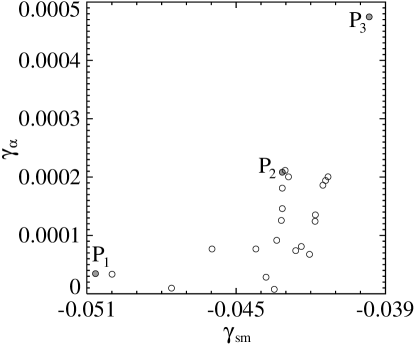
(a)   (b)  

(c)   (d)  

Figure 1: Maximum slow-time growth rates (14) of large-scale modes due to the action of the $\alpha$-effect (vertical axis) versus dominant fast-time growth rates of small-scale modes (horizontal axis) for $\eta=0.05$ in the collection of 23 family P flows (a). The topography of the vertical component for three poloidal flows (36) is shown in (a) by gray filled circles marked P₁ (b), P₂ (c) and P₃ (d). Isolines show the values step 2 of the r.m.s.-normalised factor $\nabla^{2}p(x_{1},x_{2})$ in the vertical component of sample flows. Dotted, dashed and solid lines indicate negative, zero and positive values, respectively; small ticks point in the direction of decreasing values.

Table 1: Dynamo properties of the three family P flows (36) shown in Fig. 1a by gray filled circles for $\eta=0.05$.

Flow	$\gamma_{\rm sm}$	$\gamma_{\alpha}$	$\nu_{1}$	$\nu_{2}$	$\nu_{3}$
P1	-0.05066	0.3448$\times 10^{-4}$	1.597967	7.905751	8.551576
P2	-0.04314	2.083$\times 10^{-4}$	-1.708137	3.269258	4.412460
P3	-0.03965	4.746$\times 10^{-4}$	-1.619310	1.531359	2.172698

We have computed solutions to the “nonlinear eigenvalue problem” (40), where the r.h.s. (41) involves three unknown parameters $\nu_{j}$:

$$f(g)=\nu_{1}{\rm e}^{g}+\nu_{2}{\rm e}^{-g}+\nu_{3}g^{3}.$$

For the employed resolution of $128^{2}$ Fourier harmonics, the energy spectrum decay of the solutions $g(x_{1},x_{2})$ is in the range 17–21 orders of magnitude. The same vertical profile

$$\widetilde{g}(x_{3})=1+\cos x_{3}+\sin\,2x_{3}$$

of the flow potential (39) has been employed to construct a collection of 23 sample flows. Small-scale dynamo fast-time growth rates and the maximum slow-time growth rates of large-scale modes generated by the $\alpha$-effect have been computed for $\eta$=0.05, for which none of the 23 poloidal flows (36) generates small-scale magnetic field (see Fig. 1a). For three flows, Figs. 1b-d show isolines of the fields $\nabla^{2}\,g(x_{1},x_{2})$ normalised so that their r.m.s. value is 1; by (36), they reflect the topography of vertical components of the flows. The three flows (marked by gray filled circles in Fig. 1a; see Table 1) are well separated in the plane (maximum growth rate of large-scale modes due to the $\alpha$-effect, dominant growth rate of small-scale modes). The flow represented by the left circle P₁ features the highest contrast in the component structure, but the part of the fluid volume, occupied by vigorous vertical jets, is small (see Fig. 1b); apparently, this is responsible for the minimum (over the set) ability of this flow to sustain small-scale magnetic field and to generate large-scale field by means of the $\alpha$-effect. The intermediate circle P₂ represents a flow featuring a comparable contrast, but there is a significant increase in the part of the volume where vertical motion is relatively fast (see Fig. 1c). Consequently, for this flow we observe a decrease in the fast-time decay rate of small-scale field and an increase in the slow-time growth rate of the generated large-scale field. Finally, the right circle P₃ represents the flow of the least contrast (among the three flows under discussion), but the part of the volume of relatively fast vertical motion has again increased (see Fig. 1d), accompanied by a further decrease in the decay rate of small-scale field and an increase in the slow-time growth rate of large-scale field generated by the $\alpha$-effect.

4.2 Family V₁

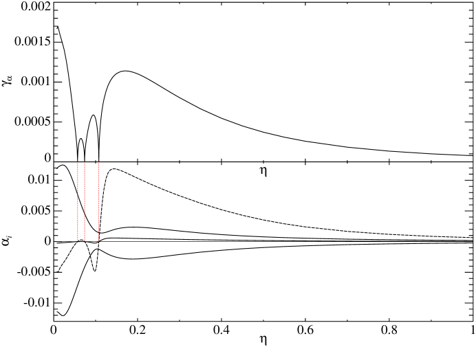
Figure 2: Upper panel: maximum slow-time growth rate of large-scale magnetic field generated by the $\alpha$-effect (vertical axis) versus magnetic molecular diffusivity $\eta$ (horizontal axis) for a sample flow from family V₁ (58) constructed for (62). Lower panel: three eigenvalues $\alpha_{i}$ of the symmetrised $\alpha$-tensor ${{}^{\rm s}\boldsymbol{\mathfrak{A}}}$ for the same flow (solid line) and the intermediate eigenvalue $\alpha_{2}$ multiplied by 20 (dashed line). Dotted vertical lines join the locations of the zero maximum growth rate due to the $\alpha$-effect with the zeroes of the intermediate eigenvalue of ${{}^{\rm s}\boldsymbol{\mathfrak{A}}}$.

We have computed slow-time growth rates $\gamma_{\alpha}$ of large-scale magnetic field generated by the $\alpha$-effect in a sample family V₁ flow (58) constructed for randomly chosen functions and constants

$$U_{1}(x_{1}) =-2\cos x_{1}+1.5\sin x_{1}+0.5\sin 2x_{1}+0.75\cos 3x_{1}-0.2\sin 3x_{1}-0.1\sin 4x_{1},$$

$$U_{2}(x_{2}) =\cos({\rm e}^{\cos 3x_{2}}-\sin 2x_{2})-0.3\sin x_{2},$$ (62)

$$U_{3}(x_{3}) =\sin x_{3}-0.75\cos 2x_{3}+0.25\cos 3x_{3}+0.2\sin 4x_{3},$$

$$C_{1} =1,\qquad C_{2}=2,\qquad C_{3}=-3.$$

For this flow, the plot of $\gamma_{\alpha}$ (see the upper panel of Fig. 2) has a rather intricate structure: by virtue of (14), it falls off to zero each time the intermediate eigenvalue $\alpha_{2}$ of the symmetrised $\alpha$-tensor ${{}^{\rm s}\boldsymbol{\mathfrak{A}}}$ vanishes (in order to visualise legibly these zeroes, the product $20\alpha_{2}$ is shown in the lower panel of Fig. 2 by a dashed line). This is reminiscent of the “window” in $\eta$, in which small-scale generation by the 1:1:1 ABC-flow fails ArK — however, in the present case intervals where there is no dynamo degenerate into individual points.

4.3 Family V₂

(a)   (b)  

(c)   (d)  

Figure 3: Maximum slow-time growth rate of large-scale magnetic field generated by the $\alpha$-effect (vertical axis) versus magnetic molecular diffusivity (horizontal axis) in the three sample flows (60) from family V₂ constructed for (63) (a), the r.m.s.-normalised functions $U_{i}$ (.4) and (64) (b), and $U_{i}$ that are Fourier series with pseudorandomly generated coefficients (c). Dots show the computed values. Plots of the three functions $U_{i}$ (.4) (d).

We plot in Fig. 3a the maximum slow-time growth rate (14) of large-scale magnetic field generated by the $\alpha$-effect in a sample flow from family V₂ (60) constructed for

$$u_{1}(x_{1}) ={\rm e}^{(\sin x_{1})/4-\cos 2x_{1}}+(\cos x_{1})/2,$$ (.1)

$$u_{2}(x_{2}) =({\rm e}^{(\sin x_{2})/4+(\cos 3x_{2})/3}+(\cos 2x_{2})/6)^{2},$$ (.2)

$$u_{3}(x_{3}) ={\rm e}^{\sin x_{3}+4\cos 3x_{3}}+5\sin 2x_{3},$$ (.3)

$$U_{i}(x_{i}) =u_{i}(x_{i})-\left\langle u_{i}(x_{i})\right\rangle,$$ (.4)

$$C_{1} =3,\qquad C_{2}=2,\qquad C_{3}=1.$$ (.5)

For the smallest molecular diffusivity $\eta=0.005$ considered for this flow, the energy spectrum of solutions to auxiliary problems of type I, ${\bf S}_{1}$, ${\bf S}_{2}$ and ${\bf S}_{3}$, decays by 5, 3 and 6 orders of magnitude in runs with the resolution of $128^{3}$ Fourier harmonics, respectively, and by 9, 7 and 9 orders in $256^{3}$ harmonics runs. Nevertheless, the discrepancy in the elements of the $\alpha$-tensor $\boldsymbol{\mathfrak{A}}$ and the maximum slow-time growth rate of large-scale field is below $2\times 10^{-8}$ (owing to the fast energy spectrum decay of the flow).

The growth rates $\gamma_{\alpha}$ for this flow are rather small (see Fig. 3a). This can be attributed to its strong anisotropy: while the amplitude of the functions $U_{1}$ and $U_{2}$ is below unity, the amplitude of $U_{3}$ is roughly 60 (see Fig. 3d); the resulting flow (60) is thus close to a plane-parallel horizontal flow that is incapable of dynamo action by the Zeldovich Zel antidynamo theorem. This has prompted us to also consider the flow (60) constructed for all

$$C_{i}=1$$ (64)

and the functions $U_{i}$ (.1)–(.4) used previously but normalised so that their r.m.s. value becomes 1. The maximum slow-time growth rates $\gamma_{\alpha}$ are about an order of magnitude higher (see Fig. 3b).

Slow-time growth rates of large-scale magnetic field generated by the $\alpha$-effect in the flow (60), (63) are also significantly smaller than those obtained for a yet another sample family V₂ flow (see Fig. 3c). It involves zero-mean functions $U_{i}$ that are Fourier series with pseudorandom coefficients for wave numbers up to 63, whose energy spectrum decays exponentially by more than 10 orders of magnitude. We have checked that no small-scale dynamo operates for the considered molecular diffusivities (by computing the dominant fast-time growth rates $\gamma_{\rm sm}$ of small-scale modes for $\eta=0.005$, 0.01, 0.02 and 0.05). A different (compared to the sample flows discussed above) behaviour of $\gamma_{\alpha}$ is observed on decreasing molecular diffusivity; however, the considered values of $\eta$ are still too high to conjecture that the saturated regime for $\eta\to 0$ has set in.

4.4 Family L

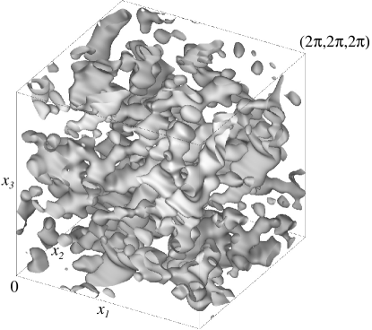
(a)     (b) 

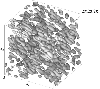
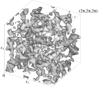
(c)     (d) 

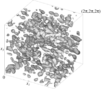
Figure 4: Isosurfaces of the flow velocity (a,c) and vorticity (b,d) at the levels of 1/3 of the respective maxima for the two sample family L flows (.2) featuring non-zero helicity spectrum, for which the magnetic $\alpha$-effect has been explored, and small-scale magnetic field generation starts in the even (a,b) or odd (c,d) invariant subspace. One periodicity cube ${\mathbb{T}}^{3}$ is shown.

(a) (b)

Figure 5: Helicity spectrum seminorm (vertical axis) versus the wave vector shell number (horizontal axis) for the two sample family L flows under consideration, in which small-scale magnetic field generation starts in the even (a) or odd (b) invariant subspace.

(a) (b)

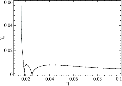
(c) (d)

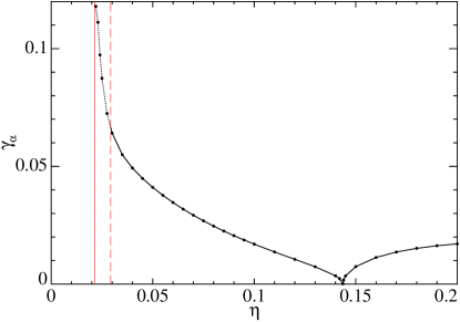
Figure 6: The fast-time growth rate (a,c) of small-scale magnetic modes (vertical axis) dominant in the even (solid line) and odd (dashed line) invariant subspaces, and the maximum slow-time growth rate $\gamma_{\alpha}$ (14) of large-scale magnetic field (b,d) generated by the $\alpha$-effect (vertical axis) versus magnetic molecular diffusivity (horizontal axes) for the two sample family L flows under consideration, where small-scale magnetic field generation starts in the even (a,b) or odd (c,d) invariant subspace. Dots show the computed values. In panels (b,d), thin vertical lines are located at the critical molecular diffusivities for the onset of the small-scale dynamo in the even (solid lines) or odd (dashed lines) subspaces. In (d), dotted line shows the part of the graph of the slow-time growth rate for $\eta$ between the critical values for the onset of small-scale generation in the two subspaces, for which large-scale generation by the $\alpha$-effect is overshadowed by the small-scale one in the odd subspace.

Two sample family L flows (.2) have been considered for the Monge potentials $A$ and $B$ that are eigenfunctions of the Laplace operator associated with the eigenvalue $-26$; they are sums of 72 Fourier harmonics, whose wave vectors are composed of numbers $\pm 3,\pm 4,\pm 1$ or of $\pm 5,0,\pm 1$, in both sets in any order and for any combination of signs. The harmonics enter the sums with complex pseudorandom coefficients (complex conjugacy is enforced for the flows to be real). Isosurfaces of the velocity $|\bf v|$ and vorticity $|\nabla\times\bf v|$ of these flows in Fig. 4 illustrate their strong spatial intermittency; Fig. 5 showing helicity spectrum seminorms

$$\Sigma_{M}=\sum_{M-1<|{\bf m}|\leq M}|H_{\bf m}|$$

furnishes evidence that the helicity spectra of the two flows do not vanish. The plots of the maximum slow-time growth rate (14) of large-scale magnetic field generated by the $\alpha$-effect, as functions of magnetic molecular diffusivity (see Fig. 6b,d), involve square-root type cusps where the growth rates vanish together with the intermediate eigenvalue $\alpha_{2}$ of the symmetrised $\alpha$-tensor ${{}^{\rm s}\boldsymbol{\mathfrak{A}}}$; this is the same phenomenon as the one seen in Fig. 2.

Notably, in Fig. 6b,d the graphs of the maximum slow-time growth rate $\gamma_{\alpha}$ have vertical asymptotes. A similar singular behaviour of eddy diffusivity was encountered (see section 3.7 in VZ ), but to the best of our knowledge it was never documented for the $\alpha$-effect. The nature of this phenomenon is the same for both mechanisms of large-scale generation, as we will now briefly discuss. Let us consider a first auxiliary problem (7) in the form of the left equation for a zero-mean solenoidal field ${\bf S}_{k}$. Generically, the magnetic induction operator $\L$ has a three-dimensional kernel spanned by the fields ${\bf e}_{k}+{\bf S}_{k}$, thus being invertible in the functional subspace of our interest. We expand, for a given $\eta$, the unknown field and the r.h.s. of the left equation (7) in the basis of solenoidal zero-mean eigenfunctions ${\bf f}_{n}(\eta)$ of the magnetic induction operator, $\L{\bf f}_{n}(\eta)=\mu_{n}(\eta){\bf f}_{n}(\eta)$:

$${\bf S}_{k}(\eta)=\sum_{n}\sigma_{nk}(\eta){\bf f}_{n}(\eta),\qquad-{\partial{\bf v}\over\partial x_{k}}=\sum_{n}\alpha_{nk}(\eta){\bf f}_{n}(\eta).$$

(For the sake of argument, we assume that $\L$ does not involve Jordan form cells of size 2 or more, although it is not difficult to take them into account in a fully formal proof.) Then, evidently,

$$\sigma_{nk}(\eta)={\alpha_{nk}(\eta)\over\mu_{n}(\eta)}\quad\Rightarrow\quad{\bf S}_{k}(\eta)=\sum_{n}{\alpha_{nk}(\eta)\over\mu_{n}(\eta)}{\bf f}_{n}(\eta);$$ (65)

while $\L$ is invertible, all $\mu_{n}(\eta)\neq 0$ and $\mu_{n}(\eta)\to-\infty$, the series thus remaining well-defined and convergent.

Suppose now $\eta\to\eta_{\rm cr}$ for the onset of the small-scale magnetic field generation, i.e., $\mu_{N}(\eta_{\rm cr})=0$ for some $N$ (corresponding in our case to the dominant mode; again, to simplify the argument, we assume that the emerging eigenvalue zero has multiplicity one; it is important that the eigenvalue at the onset is real). The eigenfunction ${\bf f}_{N}(\eta)$ remains smooth and bounded, however, the solution (65) infinitely increases, as well as the $\alpha$-effect tensor

$$\boldsymbol{\mathfrak{A}}_{k}(\eta)={\alpha_{Nk}(\eta_{\rm cr})\over\mu_{N}(\eta)}\left\langle{\bf v}\times{\bf f}_{N}(\eta_{\rm cr})\right\rangle+{\rm o}(\mu_{N}^{-1}).$$

This results in emergence of the vertical asymptote like the one shown in Fig. 6b. (Note that this may be interpreted not as “an infinite rate of generation” at $\eta=\eta_{\rm cr}$, but rather as that the ansatz (6) becomes inapplicable for the critical $\eta$. Although $|\lambda_{1}|\to\infty$ when $\eta_{\rm cr}$ is approached, Re $\lambda_{1}$ approximates the slow-time growth rate only for $\varepsilon\to 0$; for acceptable $\varepsilon$, the product $\varepsilon{\rm Re}\lambda_{1}$ approximating the fast-time growth rate remains finite, if does not tend to zero.)

There is a subtlety: the Monge potentials $A$ and $B$ defining a family L flow are linear combinations of Fourier harmonics that are eigenfunctions of the Laplacian associated with the same eigenvalue. Because of the periodicity condition, a wave vector of each harmonics has integer components, whose sum has the same parity as the Laplacian eigenvalue. Therefore, any flow (.2) belongs to what we call the “even” subspace composed of harmonics such that the sum of wave numbers is even. In the “odd” complementary subspace, the sum of wave numbers of the constituting harmonics is odd. When the flow belongs to the even subspace, even and odd subspaces are invariant for the small-scale magnetic induction operator $\L$. All neutral modes ${\bf e}_{k}+{\bf S}_{k}$ belong to the even subspace and do not “feel” the onset of small-scale field generation, when it occurs (on decreasing $\eta$) in the odd subspace. The $\alpha$-effect tensor acquires singularity, as discussed above, when the onset is in the even subspace. This happens (see Fig. 6a,b) for the sample flow shown in Fig. 4a,b. For the flow shown in Fig. 4c,d, the onset occurs in the odd subspace (see Fig. 6c) not affecting the graph of the maximum slow-time growth rate of large-scale magnetic field generated by the $\alpha$-effect Fig. 6d. (For this flow, the part of the graph of $\gamma_{\alpha}$ shown in Fig. 6d by the dotted line for $\eta$ between the critical values for the onset of small-scale generation in the two subspaces only illustrates the singular behaviour near the critical molecular diffusivity in the even subspace. As discussed in the introduction to the present section, large-scale generation, whose fast-time growth rate is order $\varepsilon$, is overshadowed in this interval by the small-scale one in the odd subspace, whose fast-time growth rate is order unity.) Actually, small-scale magnetic field generation occurs in the odd subspace more frequently than in the even one. Perhaps, the reason is in that the shortest wave vector in the even subspace is $\sqrt{2}$ times longer than the one in the odd subspace, and hence the small wave number harmonics (storing a significant part of energy of a dominant small-scale magnetic mode) are more amenable to molecular diffusion in the even subspace than in the odd one.

5 Magnetic eddy diffusivity in non-helical flows: numerical results

We have examined numerically magnetic eddy diffusivity of some instances of flows belonging to families L, C and V₁ (see subsections 3.2, 3.3 and 3.5, respectively), that are parity-invariant and hence lack the $\alpha$-effect. Family V₂ flows are not parity-invariant (see a comment to this effect at the end of section 3.5) and generically sustain the $\alpha$-effect; hence, they have been excluded here from examination. As when exploring the $\alpha$-effect, for each pair (a flow / magnetic molecular diffusivity) considered here, we have computed the fast-time growth rate $\gamma_{\rm sm}$ of the dominant small-scale magnetic mode, and in what follows we comment on the minimum magnetic eddy diffusivity (24) for flows that do not generate small-scale magnetic field. The rationale is discussed in the introduction to section 4.

Each employed flow has a unit r.m.s. velocity.

Computation of the eddy diffusivity tensor can be significantly simplified (to the extent that there may be no need to solve auxiliary problems for the adjoint operator) in the presence of certain symmetries of the flow. In particular, the symmetries of the cosine flows imply splitting of the domain of the magnetic induction operator into invariant subspaces and a special structure of the eddy diffusivity tensor. We discuss these issues in section 5.2.

5.1 Family L

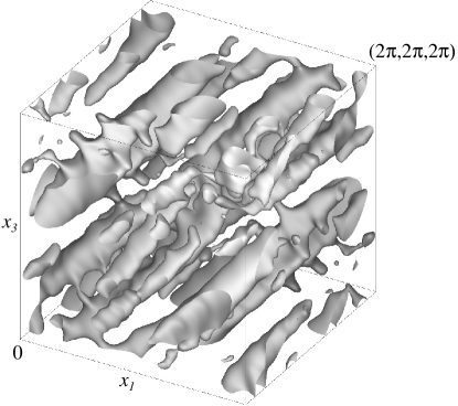
(a)        (b) 

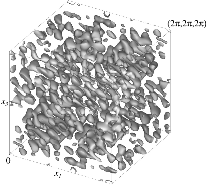
Figure 7: Isosurfaces of the flow velocity (a) and vorticity (b) at the levels of 1/3 and 2/5 of the maxima, respectively, for a sample parity-invariant family L flow (.2) for which magnetic eddy diffusivity has been explored. One periodicity cube ${\mathbb{T}}^{3}$ is shown.

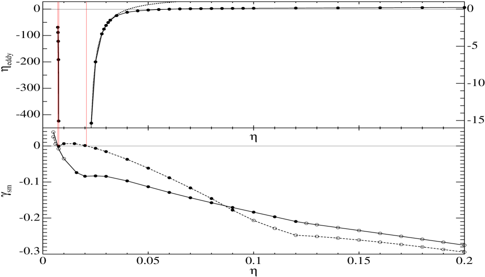
Figure 8: Upper panel: minimum magnetic eddy diffusivity $\eta_{\rm eddy}$ (vertical axes) versus molecular diffusivity $\eta$ (horizontal axis) in the sample parity-invariant family L flow (.2). Dots show the computed values. The scales for the left and right branches of the plot are shown in the left and right vertical axes, respectively. Dotted curve is the least-squares hyperbolic fit for the 7 shown values of $\eta_{\rm eddy}$ computed in the interval $0.023\leq\eta\leq 0.032$ . Lower panel: dominant fast-time growth rate of small-scale modes (vertical axis) as a function of $\eta$ for the sample flow in the invariant subspaces of parity-invariant (solid line) and parity-antiinvariant (dashed line) vector fields. Filled (hollow) circles indicate that eigenvalues of the small-scale magnetic induction operator are real (complex, respectively). Thin vertical lines are located at the critical molecular diffusivities for the onset of the small-scale dynamo in the two symmetry subspaces.

Like in section 4.4, we consider here a sample family L flow (.2) for the Monge potentials $A$ and $B$ that are eigenfunctions of the Laplace operator associated with the eigenvalue $-26$. They are again linear combinations of Fourier harmonics for wave vectors $(\pm 3,\pm 4,\pm 1)$ and permutations, as well as $(\pm 5,0,\pm 1)$ and permutations. However, the pseudorandom coefficients in the combinations are now imaginary, whereby each potential is an odd (i.e., $f(-{\bf x})=-f({\bf x})$) real scalar field, resulting in parity invariance of the flow. Isosurfaces of the flow velocity and vorticity (see Fig. 7) reveal its elaborate internal structure.

The upper panel of Fig. 8 presents the minimum magnetic eddy diffusivity (24) for this flow as a function of the magnetic molecular eddy diffusivity $\eta$. For $\eta$ sufficiently large, $\eta_{\rm eddy}>0$, but on decreasing molecular diffusivity $\eta_{\rm eddy}$ changes the sign near $\eta\approx 0.0612$. The plot of $\eta_{\rm eddy}$ has a vertical asymptote located at the critical molecular diffusivity $\eta_{\rm cr}\approx 0.0207$ for the onset of the small-scale magnetic field generation (see the lower panel of Fig. 8). Section 3.7 of VZ explains this phenomenon: solutions to the auxiliary problems involve the inverse small-scale magnetic induction operator $\L^{-1}$; in short, when $\eta$ is close to $\eta_{\rm cr}$, the norm of $\L^{-1}$ is large, and thus either solutions to auxiliary problems of type II are large (if the neutral zero-mean magnetic mode emerging at $\eta=\eta_{\rm cr}$ is parity-invariant), or solutions to all auxiliary problems are large (if the mode is parity-antiinvariant). As an illustration, we have also plotted by a dotted line the least-square hyperbolic fit (the ratio of two linear functions) obtained for the seven computed values of $\eta_{\rm eddy}$ in the interval $0.023\leq\eta\leq 0.032$ . The position of the vertical asymptote of the fit, at the zero of the denominator, differs from the linearly estimated critical molecular diffusivity $\eta_{c}\approx 0.0207$ by less then $10^{-4}$.

Small-scale parity-antiinvariant magnetic field is generated for $0.0077\apprle\eta\apprle 0.0207$. For smaller $\eta$ in the adjacent interval $0.0063\apprle\eta\apprle 0.0077$, generation in this symmetry subspace ceases. This is analogous to the window where the 1:1:1 ABC-flow does not act as a small-scale kinematic dynamo ArK . Inside this interval, at $\eta\approx 0.0064$, the branch of dominant parity-antiinvariant magnetic modes is replaced by a different one: the associated eigenvalues change from real (for large $\eta$) to complex ones (for small $\eta$), the imaginary part of the dominant eigenvalue experiencing a jump. In the same interval, at $\eta\approx 0.0071$, generation of small-scale parity-invariant field sets in. (All the critical values have been determined by linear interpolation of real parts of the computed eigenvalues.)

Thus, no small-scale generation takes place in a short interval $0.0071\apprle\eta\apprle 0.0077$ . At the right endpoint of this interval, $\eta\approx 0.0077$, there exists a neutral (i.e., the associated eigenvalue of the magnetic induction operator is 0) parity-antiinvariant zero-mean small-scale magnetic mode. By the same argument as for $\eta_{c}\approx 0.0207$, the endpoint hosts another singularity of $\eta_{\rm eddy}$. The minimum eddy diffusivity tends to $-\infty$ on increasing $\eta$ towards the right endpoint $\eta\approx 0.0077$ (see the left branch of the plot in the upper panel of Fig. 8). Thus, we have encountered an example of a flow that has at least two windows in magnetic molecular diffusivity where no small-scale magnetic field is generated, but generation of large-scale field does take place. At $\eta\approx 0.0063$, the increment of magnetic field also vanishes, but the respective eigenvalue of the magnetic induction operator has a non-zero imaginary part, and consequently $\eta_{\rm eddy}$ remains non-singular.

5.2 Cosine flows: family C

Numerical investigation of eddy diffusivity of the cosine flows (47) is significantly simplified by their two properties: translation by half the period in the vertical direction reverses the flows, and they are symmetric in $x_{3}$.

If translation by a vector $\bf a$ reverses the flow,

$$\bf v(x+a)=-v(x)$$ (66)

($|\bf a|$ is then a half of the smallest period in the direction of $\bf a$), then by virtue of (7) and (18)

$${\bf S}^{-}_{l}({\bf x})={\bf S}_{l}({\bf x+a})$$ (67)

for all $l$. Thus, for such flows it suffices to solve the 3 auxiliary problems (7) of type I. For the cosine flows (47) this happens for ${\bf a}=(\pi/n)\,{\bf e}_{3}$.

Furthermore, following ABNZ , we use (66), (27) and (67) for the index $k$ instead of $l$ to transform (25) into

$$\boldsymbol{\mathfrak{D}}^{l}_{mk}=\eta\int_{{\mathbb{T}}^{3}}{\bf Z}_{l}({\bf x})\cdot\left(2\,\nabla\times{\partial\over\partial x_{m}}{\bf Z}_{k}({\bf x+a})-{\bf e}_{m}\times\nabla^{2}{\bf Z}_{k}({\bf x+a})\right)\,{{\rm d}{\bf x}\over(2\pi)^{3}}.$$

Integrating here by parts the first scalar product and exploiting self-adjointness of the Laplacian and the curl, as well as the antisymmetry of the triple product with respect to permutation of its factors, we find that

$$\mathfrak{D}^{l}_{mk}=-\mathfrak{D}^{k}_{ml}\qquad\Rightarrow\qquad\mathfrak{D}^{k}_{mk}=0$$

for all indices $l,m,k$. Therefore, ${{}^{\rm s}\!D}=0$ implying $d=0$, and for any wave vector $\bf q$ eigenvalues (23) of the eddy diffusivity operator are two-fold.

A field ${\bf f}=(f^{1},f^{2},f^{3})$ is called symmetric in $x_{i}$, if for all $i$ and $j$

$$f^{j}((-1)^{\delta^{1}_{i}}x_{1},(-1)^{\delta^{2}_{i}}x_{2},(-1)^{\delta^{3}_{i}}x_{3})=(-1)^{\delta^{j}_{i}}\,f^{j}({\bf x})$$

and antisymmetric in $x_{i}$, if for all $i$ and $j$

$$f^{j}((-1)^{\delta^{1}_{i}}x_{1},(-1)^{\delta^{2}_{i}}x_{2},(-1)^{\delta^{3}_{i}}x_{3})=(-1)^{1-\delta^{j}_{i}}\,f^{j}({\bf x}).$$

The symmetry in $x_{i}$ of the flow $\bf v$ implies that vector fields symmetric or antisymmetric in $x_{i}$ constitute invariant subspaces of the magnetic induction operator $\L$ (4). It is then evident from (7) and (26) that for the cosine flows
$\bullet$ ${\bf S}_{k}$ is symmetric in $x_{3}$ for $k=1,2$ and antisymmetric in $x_{3}$ for $k=3$;
$\bullet$ ${\bf Z}_{l}$ is antisymmetric in $x_{3}$ for $l=1,2$ and symmetric in $x_{3}$ for $l=3$.
Consequently, by (25), $\mathfrak{D}^{l}_{mk}=0$ if all indices $l,m,k$ do not exceed 2, or precisely two of them are equal to 3.

Thus, eddy diffusivity tensor $\boldsymbol{\mathfrak{D}}$ for a cosine flow involves 5 pairs of non-zero entries of opposite signs, and by virtue of (23)

$$\lambda_{2}({\bf q})=-\eta+\mathfrak{D}^{2}_{31}\cos^{2}\theta+\sin^{2}\theta\left(\mathfrak{D}^{3}_{12}\cos^{2}\varphi+(\mathfrak{D}^{3}_{22}+\mathfrak{D}^{1}_{13})\cos\varphi\sin\varphi+\mathfrak{D}^{1}_{23}\sin^{2}\varphi\right)$$

for the wave vector (.1). The minimum eddy diffusivity (24) is now

$$\eta_{\rm eddy}=\eta-\max\left(\mathfrak{D}^{2}_{31},\ {1\over 2}\left(\mathfrak{D}^{3}_{12}+\mathfrak{D}^{1}_{23}+\sqrt{(\mathfrak{D}^{3}_{12}-\mathfrak{D}^{1}_{23})^{2}+(\mathfrak{D}^{3}_{22}+\mathfrak{D}^{1}_{13})^{2}}\right)\right).$$

We have investigated magnetic eddy diffusivity for a set of cosine flows that satisfy the following conditions:
$\bullet$ The horizontal vectors ${\bf a}=(a_{1},a_{2},0)\neq 0$ and ${\bf b}=(b_{1},b_{2},0)\neq 0$ have integer components, $|a_{i}|\leq 3$, $|b_{i}|\leq 3$; $n\leq 3$ is a positive integer.
$\bullet$ $\bf a$ and $\bf b$ are neither orthogonal, nor parallel. (If ${\bf a\cdot b}=0$, the vertical component of (47) vanishes identically; such flows are irrelevant for us, since by the Zeldovich Zel antidynamo theorem a planar flow cannot generate magnetic field. For parallel $\bf a$ and $\bf b$, the flow is also planar: ${\bf v}\cdot(b_{2},-b_{1},0)=0$.)
$\bullet$ The largest common divisor of four integers $a_{i}$ and $b_{i}$ is 1, so that the flow does not have a smaller horizontal periodicity cell aligned with the coordinate axes.
$\bullet$ No pair $\bf a,b$ used for construction of a flow in the set is derived from another such pair by performing the following transformations or their compositions:
$(i)$ swapping $\bf a\leftrightarrow\bf b$ (this does not alter the flow);
$(ii)$ inverting the signs $\bf a\to-a$ or $\bf b\to-b$ (the flow is invariant under any of the two reversals simultaneously with a shift in half a period $\pi/n$ in $x_{3}$);
$(iii)$ swapping the components $a_{1}\leftrightarrow a_{2}$ and $b_{1}\leftrightarrow b_{2}$ (flows obtained for two such pairs $\bf a,b$ map into each other under swapping of the horizontal components of vector fields and of the horizontal Cartesian axes, $x_{1}\leftrightarrow x_{2}$);
$(iv)$ for some $i\leq 2$, inverting the signs of $a_{i}\to-a_{i}$ and $b_{i}\to-b_{i}$ (a flow remains invariant under this inversion accompanied by reflection of the direction $x_{i}\to-x_{i}$ and changing the sign of the $i$th component of vector fields).

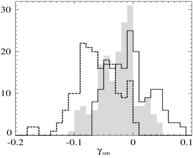
(a)         (b)  

(c)         (d)  

Figure 9: Histogram of dominant fast-time growth rates of small-scale magnetic modes generated by the 183 primary cosine flows (a) for three values of magnetic molecular diffusivity: $\eta=0.01$ (black solid line), 0.02 (gray solid line, the area below the plot is filled in gray), 0.05 (dashed line). Histograms of the minimum magnetic eddy diffusivity in the 183 primary cosine flows (solid line) and for those of them which are not small-scale dynamos (dashed line) for $\eta=0.01$ (b), 0.02 (c) and 0.05 (d).

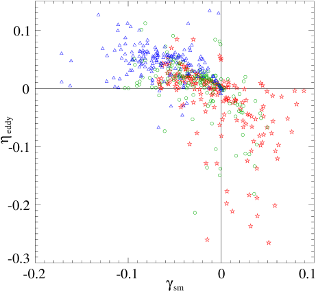
Figure 10: Minimum eddy diffusivity $\eta_{\rm eddy}$ (vertical axis) versus dominant fast-time growth rates of small-scale modes (horizontal axis) in the primary cosine flows (47) for three values of magnetic molecular diffusivity: $\eta=0.01$ (stars), 0.02 (circles) and 0.05 (triangles).

Figure 11: Minimum magnetic eddy diffusivity (vertical axis) in a family V₁ sample flow (58) versus the magnetic eddy diffusivity $\eta$ (horizontal axis). Dots show the computed values.

Table 2: Primary cosine flows as small- and large-scale dynamos. Columns 1-4 present numbers of the primary cosine flows (47) in the specified classes for two values of magnetic molecular diffusivity.

	$\eta=0.01$		$\eta=0.02$
	$\eta_{\rm eddy}<0$	$\eta_{\rm eddy}>0$	$\eta_{\rm eddy}<0$	$\eta_{\rm eddy}>0$
Small-scale dynamo	61	12	27	134
No small-scale generation	25	85	20	132

This set of essentially distinct low-wavenumber cosine flows comprises 183 flows, which we will call primary cosine flows. The distribution of the dominant fast-time growth rates of small-scale magnetic field and of the minimum eddy diffusivity computed for these flows is shown in Figs. 11 and 11 for three values of molecular diffusivity, $\eta=0.01$, 0.02 and 0.05 (see also Table 2). While a significant proportion of the primary flows is capable of generating small-scale magnetic field for $\eta\leq 0.02$, only three instances of them are small-scale dynamos for $\eta=0.05$. This value is also close to the upper bound of $\eta$, for which large-scale generation by the cosine flows is possible: for $\eta=0.05$, only 11 instances of primary cosine flows feature negative magnetic eddy diffusivity, including the 3 flows that can generate small-scale field.

The most populated class (consisting of more than a half of the total number of flows for all considered $\eta$) are the primary cosine flows that are neither small-, nor large-scale dynamos (quadrant II in Fig. 11). By contrast, for $\eta=0.01$ and 0.02, the second largest class are flows that sustain both small- and large-scale (by the mechanism of negative eddy diffusivity) generation (quadrant IV in Fig. 11). Nevertheless, for these values of molecular diffusivity, there are quite a few primary cosine flows of our prime interest, that are incapable of small-scale generation but feature negative eddy diffusivity (quadrant III in Fig. 11). Finally, for both $\eta$, the least numerous is the class of flows that can generate small-scale flows, but give rise only to positive eddy diffusivity (quadrant I in Fig. 11). For each of the three classes of flows that sustain at least one of the two considered types of generation, the cardinality falls when molecular diffusivity increases from $\eta=0.01$ to 0.02; this agrees with the “common sense” argument that enhancing magnetic molecular diffusivity hinders the ability to generate magnetic field.

5.3 Family V₁

The minimum magnetic eddy diffusivity in a family V₁ sample flow (58) constructed for $C_{1}=1$, $C_{2}=1,\ C_{3}=-2$ is shown in Fig. 11. The functions $U_{i}(x_{i})$ have been synthesised as Fourier series with zero coefficients for the wave numbers $|n|>10$ and $n=0$. The coefficients for $0<n\leq 10$ have been assigned the imaginary values ${\rm i}6^{-n}r_{n}$, where $r_{n}$ is a pseudorandom real number in the interval $[0,1]$, and complex-conjugate values are employed for $n<0$. The energy spectrum of the resultant flow decays by 10 orders of magnitude. By construction, all $U_{i}(x_{i})$ are odd, whereby (58) is a parity-invariant flow.

We observe a typical behaviour of the minimum eddy diffusivity (24): $\eta_{\rm eddy}>0$ for sufficiently large molecular diffusivity $\eta$, but $\eta_{\rm eddy}<0$ and thus large-scale generation becomes possible below a certain $\eta>0$. The minimum eddy diffusivity tends to $-\infty$ when $\eta$ approaches the critical value for the onset of the small-scale generation (see section 3.7 of VZ ).

6 Concluding remarks

1. We have presented (section 3) six families of pointwise non-helical (i.e., satisfying (2)) steady space-periodic three-dimensional flows of incompressible fluid. One, family P (see section 3.1), consists of poloidal flows. For determining the potentials $P({\bf x})$ (39) for certain such flows, we propose to solve the two-dimensional scalar problems (40)–(41) “of the nonlinear eigenvalue type”. Four families (C, L, V₁ and V₂) are analytically defined. This has provided enough flows to conduct numerical experiments in magnetic field generation. However, it is desirable to find methods for constructing pointwise zero-helicity solenoidal flows, whose streamlines involve knots of a given topology, in the spirit of KFDI .

Furthermore, we have shown (section 3.6) that flows comprising families P, C, V₁ and V₂ have zero helicity spectrum.

2. In application of the multiscale formalism (see VZ ) to the problem of kinematic generation of large-scale magnetic field by small-scale flows in the limit of high scale separation, eigenfunctions and the associated eigenvalues of the large-scale magnetic induction operator are expanded in the power series (6) in the scale ratio $\varepsilon$. Generically, the $\alpha$-effect is present, and the leading term in expansion of the eigenvalue is $\varepsilon\lambda_{1}$, where $\lambda_{1}$ is an eigenvalue of the magnetic $\alpha$-effect operator (see (8)). For an arbitrary unit (large-scale) wave vector $\bf q$, we have derived the eigenvalues $\lambda_{1}$ (13) associated with the harmonic eigenfunctions (10), as well as the maximum, over unit $\bf q$, slow-time growth rate (14) sustained by the action of the $\alpha$-effect. The growth rate is controlled by the symmetric part of the $\alpha$-effect tensor, $\boldsymbol{\mathfrak{A}}$. We have also proven that the $\alpha$-effect tensor $\boldsymbol{\mathfrak{A}}^{-}$ for the reverse flow $-\bf v(x)$ is obtained from the tensor $\boldsymbol{\mathfrak{A}}$ for $\bf v(x)$ by matrix transposition.

When the $\alpha$-effect is absent ($\boldsymbol{\mathfrak{A}}=0$), the leading term in the expansion of the eigenvalue is $\varepsilon^{2}\lambda_{2}$, where $\lambda_{2}$ is an eigenvalue of the magnetic eddy diffusivity operator (see (21)). We have calculated the eigenvalues $\lambda_{2}$ (23) associated with the harmonic eigenfunctions (10). (To the best of our knowledge, the relations (13) and (23) were so far unavailable in the literature; however, see section 9.3 in Mb .)

3. We have computed (section 4) the maximum (over the direction of the wave vector $\bf q$) slow-time growth rates Re $\lambda_{1}$ due to the action of the magnetic $\alpha$-effect in sample flows from families P, V₁, V₂ and L (defined in sections 3.1, 3.5 and 3.2), as well as (section 5) the maximum slow-time growth rates Re $\lambda_{2}$ sustained by the magnetic eddy diffusivity in sample flows from families L, C (defined in section 3.3) and V₁. (Family C cosine flows are parity-invariant and thus lack the $\alpha$-effect; by contrast, no family V₂ flows are parity-invariant and might be used to investigate magnetic eddy diffusivity.)

In all considered families we have encountered flows that, for sufficiently small magnetic molecular diffusivities, $\eta$, generate large-scale magnetic field by employing the respective mechanism. In addition, in all the families we have found sample flows that generate small-scale field. Thus, we have demonstrated that zero kinetic helicity density does not rule out generation of large-scale magnetic field by the mechanisms of the $\alpha$-effect or negative magnetic eddy diffusivity, and of small-scale field. This can be explained heuristically as follows: Various topological properties of knottedness of vorticity lines are controlled by the independent quantities $\cal W$, $\cal T$ and $\cal N$, whose sum $n$ enters the kinetic helicity (1) as a factor. Zero helicity does not require vanishing of any of these quantities, and non-zero values indicate that the lines possess non-trivial respective knottedness properties. This implies an intricate topological structure of the non-helical flow that, empirically, is likely to give rise to generation of magnetic field.

Actually, from this perspective the flow helicity rather than the kinetic helicity (which is the vorticity helicity) seems to be more appropriate for characterising the flow complexity significant for magnetic field generation. Indeed, in the limit of small local magnetic Reynolds numbers, in view of the relation

$${\rm tr}\,\boldsymbol{\mathfrak{A}}=-\eta^{-1}\left\langle{\bf v}\cdot(-\nabla\times\nabla^{-2}{\bf v})\right\rangle+{\rm O}(\eta^{-2})$$

for the tensor (28) (see also chapters 10 and 11 of VZ ), the $\alpha$-effect is directly linked with the flow helicity equal to the spatial mean in the r.h.s. Furthermore, the same expression (up to the O($\eta^{-2}$) term) was found for the trace of the $\alpha$-effect tensor in the mean-field electrodynamics (see RBr and references therein) in the low-conductivity limit, and the mean flow helicity was claimed to play a fundamental role for the dynamo action of the $\alpha$-effect especially for steady flow (cf. expression (33) for the $\alpha$-effect tensor for time-periodic flow). Consequently, a numerical investigation analogous to the present one is desirable, in which the $\alpha$-effect and eddy diffusivity tensors, (9) and (22), respectively, will be studied numerically for a set of steady three-dimensional space-periodic solenoidal flows, whose flow helicity density vanishes pointwise.

4. Hydrodynamic helicity exists in two loosely related incarnations: kinetic helicity with the density ${\bf v}\cdot\nabla\times{\bf v}$, which is mainly of our concern in the present work, and the helicity spectrum (34), which can be regarded as a kind of helicity density in the Fourier space. It was shown in the theory of mean-field electrodynamics that a non-zero helicity spectrum is necessary for the action of the $\alpha$-effect under certain conditions M70 ; MP . Asymptotic multiscale methods (see section 2.3) yield the same conclusion and the same expression for the $\alpha$-effect tensor in the limit of small R${}_{m}^{\rm loc}$.

However, our numerical results demonstrate that for finite (non-vanishing) R${}_{m}^{\rm loc}$ a non-zero helicity spectrum is required neither for the action of small-scale dynamo, nor for generation of large-scale field. Although flows comprising families P, C, V₁ and V₂ have an identically vanishing helicity spectrum (see section 3.6), computations attest that this does not result in vanishing of the $\alpha$-effect tensor and does not prevent the $\alpha$-effect from generation. We also observe that the helicity spectrum is zero for all parity-invariant flows, but nevertheless they can sustain negative eddy diffusivity.

Thus, all flows that we consider numerically feature a zero kinetic helicity density and zero helicity spectrum, except for two instances of family L flows discussed in section 4.4, whose helicity spectrum (but not kinetic helicity density) are non-zero. The slow-time growth rates of large-scale magnetic fields that they generate are roughly an order of magnitude higher than the slow-time growth rates due to the action of the $\alpha$-effect in other flows that we have considered, but it is unclear whether this is just a coincidence (the influence of the singularities in the graphs Fig. 6), or indeed generation becomes more vigorous under the influence of a non-zero helicity spectrum. Following the anonymous First Referee, we can formulate a conclusion as a relaxed modification of the title of GFP : helicity is unnecessary for dynamo action, but it may help.

Kinetic helicity and helicity spectrum turn out to be unsatisfactory measures of the flow chirality deemed necessary for generation, except in certain limit cases. By analogy, we doubt that any helicity-type integral quantity can serve for predicting the ability of a steady flow to generate a small- or large-scale magnetic field, except in specific limits — as the helicity spectrum becomes necessary for persistence of the $\alpha$-effect when R${}_{m}^{\rm loc}\to 0$. Any such criterion is unlikely to be useful, just predicting that under certain conditions the first term in the respective expansion of the eigenvalue of the induction operator vanishes — in which case generation may still be made possible by virtue of subleading terms (e.g., in the absence of the $\alpha$-effect generation may still be powered by negative eddy diffusivity).

Magnetic analogues of the kinetic helicity and helicity spectrum do show up in the mathematical multiscale kinematic dynamo theory. The $\alpha$-effect tensor (9) can be decomposed as

$$\boldsymbol{\mathfrak{A}}_{k}={\rm i}\sum_{{\bf n}\neq 0}|{\bf n}|^{-1}H_{\bf n}^{{\bf v,S}_{k}},$$ (68)

where

$$H_{\bf n}^{{\bf v,S}_{k}}=\overline{\hat{\bf v}}_{\bf n}\cdot({\rm i}{\bf n}\times{\hat{\bf S}}_{k,\bf n})$$

can be interpreted as the cross-helicity spectrum of the flow $\bf v$ and neutral magnetic mode ${\bf S}_{k}$ (their Fourier coefficients are denoted by ${\hat{\bf v}}_{\bf n}$ and ${\hat{\bf S}}_{k,\bf n}$, respectively). In view of the relations (16) (to the best of our knowledge discovered in VZ ), helicities of the currents $\nabla\times{\bf S}_{k}$ associated with small-scale neutral modes of the magnetic induction operator $\L$ are also more appropriate than the kinetic helicity or helicity spectrum for characterising the magnetic $\alpha$-effect: in the limit of high spatial scale separation, (68) and (16) hold true for any local magnetic Reynolds number and not just for R${}_{m}^{\rm loc}\to 0$. However, such identities just manifest the mathematical fact that the mean vector product of two solenoidal space-periodic fields is a linear functional of their cross-helicity spectrum; we doubt that this reveals any physical significance of their helicity spectra. The $\alpha$-effect tensor does vanish when all $H_{\bf n}^{{\bf v,S}_{k}}=0$, but to check this we must compute the neutral modes ${\bf S}_{k}$ — and afterwards it is straightforward to directly compute the tensor (9).

5. The maximum slow-time growth rate (14) due to the action of the magnetic $\alpha$-effect is non-negative; it vanishes if and only if the intermediate eigenvalue $\alpha_{2}$ of the symmetrised $\alpha$-effect tensor ${{}^{\rm s}\boldsymbol{\mathfrak{A}}}$ is zero. Figure 2 demonstrates that on decreasing $\eta$ there can be quite a few points, where $\alpha_{2}=0$. Thus, the maximum growth rate (14) may be expected to exhibit an intermittent behaviour analogous to the one shown in Fig. 2, with strictly positive values separated by zero for infinitely many $\eta$’s accumulating at $\eta=0$.

6. It is known that magnetic eddy diffusivity can become infinitely negative when magnetic molecular diffusivity approaches the critical value $\eta\to\eta_{\rm cr}$ for the onset of the small-scale dynamo action, and we have encountered such behaviour in the present work. When considering generation of large-scale magnetic field by the magnetic $\alpha$-effect, we have come across a similar infinite increase of the maximum slow-time growth rate $\gamma_{\alpha}$ (14) in the limit $\eta\to\eta_{\rm cr}$ (see Fig. 6b). The two phenomena have the same nature. We have explained such a singular behaviour of $\gamma_{\alpha}$ by considering expansions of the fluctuating part ${\bf S}_{k}$ of neutral modes in the basis of eigenfunctions of the small-scale magnetic induction operator $\L$.

7. We have encountered an instance of two disjoint intervals of magnetic molecular diffusivity where small-scale generation is absent, but large-scale magnetic field is generated by the mechanism of negative magnetic eddy diffusivity. The window between these two intervals, where no large-scale generation happens, may be regarded as a large-scale dynamo counterpart to the window of quiescence of the small-scale kinematic dynamo action by the 1:1:1 ABC-flow discovered in ArK .

8. Are our dynamos fast or slow? Families V₁ (58) and V₂ (60) flows are integrable (to see this, introduce a new time $\tau$ satisfying ${\rm d}\tau/{\rm d}t=\dot{U}_{1}\dot{U}_{2}\dot{U}_{3}$ for a V₁ flow or ${\rm d}\tau/{\rm d}t=U_{1}U_{2}U_{3}$ for a V₂ flow). Therefore, they cannot act as fast dynamos, because this requires chaotic behaviour of fluid particle trajectories and positiveness of topological entropy of the flow KY (see also V89 ; So ). Equally, trajectories of a cosine flow (47) and of a family P flow (36) for the potential (39) lie on vertical cylindrical surfaces, whose intersection with a horizontal plane can be found by considering the ratio of the two differential equations for horizontal coordinates of a fluid particle. This rules out chaos. For other family P flows and for family L flows a more detailed study of integrability and chaotic properties is required.

We can examine this question from a different perspective. Computations suggest that for the molecular diffusivity $\eta$ tending to zero, the small-scale neutral modes ${\bf S}_{k}+{\bf e}_{l}$ (and their reverse-flow counterparts ${\bf S}^{-}_{l}+{\bf e}_{l}$) grow in amplitude. In view of (9), the magnitude of the $\alpha$-effect tensor is an outcome of the competition of this growth and the decay of the energy spectrum of the smooth flow $\bf v$. Also, we observe in ${\bf S}_{k}$ a shift of the maximum of the energy spectrum towards large wave vectors; if it occurs simultaneously with a similar shift in ${\bf S}^{-}_{l}$, then by (25) and (27) the magnitude of the eddy diffusivity tensor may increase in this limit (although the definition (22) does not make this obvious). Consequently, a fast (in the respective slow time) dynamo is apparently not ruled out for both mechanisms of large-scale generation. However, a version of the argument presented in section 4.4 is applicable: the growth rates measured in the fast time are approximated by the leading terms in (.2), $\varepsilon$Re$\,\lambda_{1}$ for the $\alpha$-effect dynamos and $\varepsilon^{2}$Re$\,\lambda_{2}$ for the eddy diffusivity dynamos, for sufficiently small $\varepsilon$ only. Bounds for such relevant $\varepsilon$ on varying $\eta$ are an open question; the growth rates observed in the fast time for these $\varepsilon$ are likely to tend to zero even if $\lambda_{1}$ or $\lambda_{2}$, respectively, increase when $\eta\to 0$.

9. How will the subsequent nonlinear evolution modify our findings about kinematic generation? This is affected by many factors.

Will kinetic helicity density remain zero? Even in the purely hydrodynamic (in the absence of magnetic field) nonlinear evolution of ideal fluid flow governed by the Euler equation, nothing prevents the flow from losing this property: it is only guaranteed, as we have mentioned in the introduction, that the mean kinetic helicity stored in any volume, whose boundary is everywhere tangent to the vorticity (including the periodicity cell which can be regarded as having no boundary), does not change in time and will thus remain zero. However, the presence of the Lorentz force and/or viscosity renders inapplicable this conservation law. The flow is likely to acquire non-zero helicity density — thus making inappropriate the question that we address in the present work.

How long will the magnetic field remain multiscale? This is an intriguing open question, which can be fully solved by direct numerical simulations only. We expect the scale separation to persist while the MHD perturbation remains weakly nonlinear. A study of amplitude equations for a large-scale weakly nonlinear perturbation of a small-scale convective dynamo CZ has revealed that the amplitudes governing the perturbation blow up at a finite slow time. This does not mean that the perturbation itself develops a singularity — just the asymptotic expansion ceases to be applicable when the perturbation becomes too strong — but perhaps suggests an abrupt transition to a regime without scale separation. Other reasons may also be responsible for transformation of a multiscale field into one with a continuous distribution of scales. A magnetic perturbation composed of a unique mode (.1) is a mathematical idealisation: In a physical system many such modes corresponding to different integer (taking into account the periodicity) multiples of the scale ratio $\varepsilon$ are present due to noise and emerge, because the magnetic perturbation is coupled with the hydrodynamic one; the same is true for digital simulations, in which the noise is due to round-off errors. The larger is the integer factor, the larger is the slow-time growth rate (.2) of the mode. Thus, competition of large-scale magnetic modes sets in, in which the modes of smaller spatial periods have higher chances to win. Together with the inverse cascade, this will apparently destroy the multiscale nature of the magnetic field.

Will magnetic field generation continue and will magnetic field persist? Simulations of various nonlinear small-scale convective dynamos attest that most different scenarios are possible: upon modification by the Lorentz force due to the growing magnetic field, the flow can settle to a non-generating hydrodynamic attractor, and in such a “self-extinguishing dynamo” magnetic field decays to zero DS ; alternatively, the MHD regime can saturate to a stable MHD steady or periodic state CGPZ ; or it may consist of a chaotic sequence of visits to formerly attracting hydrodynamic states, some of which can generate magnetic field, and other ones cannot, thus exhibiting intermittent upsurges and decays of magnetic field CRC ; or the evolution can consist of a chaotic sequence of visits to unstable but identifiable MHD states — a scenario Pod for development of magnetic field reversals is an example; or it can be just an unstructured chaotic trajectory in the phase space. In any case, when the overcriticality is not too small, the initial flow is abandoned, rendering inapplicable our analysis.

References

References

- (1) Andrievsky A., Brandenburg A., Noullez A., Zheligovsky V. Negative magnetic eddy diffusivities from test-field method and multiscale stability theory. Astrophys. J. 811, 135 (2015) [http://arxiv.org/abs/1501.04465].
- (2) Arnold V.I. Sur la topologie des écoulements stationnaires des fluides parfaits. C. R. hebd. séanc. Acad. Sci. Paris, 261, 17–20 (1965).
- (3) Arnold V.I., Khesin B.A. Topological methods in hydrodynamics. Applied mathematical sciences, 125. Springer-Verlag, NY, 1998.
- (4) Arnold V.I., Korkina E.I. The growth of a magnetic field in a three-dimensional incompressible flow. Vestnik Moscow State Univ. Ser. Math. (3), 43–46 (1983) (in Russian).
- (5) Biferale L., Crisanti A., Vergassola M., Vulpiani A. Eddy diffusivities in scalar transport. Phys. Fluids. 7, 2725–2734 (1995).
- (6) Chertovskih R., Gama S.M.A., Podvigina O., Zheligovsky V. Dependence of magnetic field generation by thermal convection on the rotation rate: a case study. Physica D, 239, 1188–1209 (2010) [arxiv.org/abs/0908.1891].
- (7) Chertovskih R., Rempel E.L., Chimanski E.V. Magnetic field generation by intermittent convection. Phys. Lett. A, 381, 3300–3306 (2017) [arxiv.org/abs/1608.04716].
- (8) Chertovskih R., Zheligovsky V. Large-scale weakly nonlinear perturbations of convective magnetic dynamos in a rotating layer. Physica D, 313, 99–116 (2015) [arxiv.org/abs/1504.06856].
- (9) Christopherson D.G. A note on the vibration of membranes. Quart. J. Math. 11, 63–65 (1940).
- (10) Demircan A., Seehafer N. Dynamos in rotating and nonrotating convection in the form of asymmetric squares. In: Dynamo and dynamics, a mathematical challenge. Proc. NATO Advanced research workshop, Cargese, France, 21-26 August, 2000. NATO Science series II: Mathematics, physics and chemistry, 26. Eds. P. Chossat, D. Ambruster, I. Oprea. Kluwer Academic Publishers, 2001, 163–171.
- (11) Fokkema D.R. Subroutine BISTBL, 1995 [http://www.staff.science.uu.nl/vorst102/software. html].
- (12) Getling A.V. The helicity of the velocity field for cellular convection in a rotating layer. Astronomicheskii Zhurnal, 89 (5), 441–448 (2012). Engl. transl.: Astronomy Reports, 56, 395–402 (2012).
- (13) Gilbert A.D., Frisch U., Pouquet A. Helicity is unnecessary for alpha effect dynamos, but it helps. Geophys. Astrophys. Fluid Dynamics, 42, 151–161 (1988).
- (14) Graham J.P., Blackman E.G., Mininni P.D., Pouquet A. Not much helicity is needed to drive large-scale dynamos. Phys. Rev. E, 85, 066406 (2012).
- (15) Kedia H., Foster D., Dennis M.R., Irvine W.T.M. Weaving knotted vector fields with tunable helicity. Phys. Rev. Lett. 117, 274501 (2016).
- (16) Khesin B.A., Chekanov Yu.V. Invariants of the Euler equations for ideal or barotropic hydrodynamics and superconductivity in D dimensions. Physica D, 40, 119–131 (1989).
- (17) Klapper I., Young L.S. Rigorous bounds on the fast dynamo growth rate involving topological entropy. Communications Math. Phys. 173, 623–646 (1995) .
- (18) Krause F., Rädler K.-H. Mean-field magnetohydrodynamics and dynamo theory. Academic-Verlag, Berlin, 1980.
- (19) Lamb H. Hydrodynamics. Cambridge Univ. Press, 1932.
- (20) Levina G.V., Burylov I.A. Numerical simulation of helical-vortex effects in Rayleigh-Bénard convection. Nonlin. Processes Geophys. 13, 205–222 (2006).
- (21) Matthews P.C. Dynamo action in convection. In: Stellar dynamos: nonlinearity and chaotic flows. ASP Conference Series, 178. Eds. M. Núñez, A. Ferriz-Mas. Astronomical Society of the Pacific, San Francisco, 1999, 107–117.
- (22) Moffatt H.K. The degree of knottedness of tangled vortex lines. J. Fluid Mech. 35, 117–129 (1969).
- (23) Moffatt H.K. Turbulent dynamo action at low magnetic Reynolds number. J. Fluid Mech. 41, 435–452 (1970).
- (24) Moffatt H.K. The mean electromotive force generated by turbulence in the limit of perfect conductivity. J. Fluid Mech. 65, 1–10 (1974).
- (25) Moffatt H.K. Magnetic field generation in electrically conducting fluids. Cambridge Univ. Press, 1978.
- (26) Moffatt H.K. Helicity and celestial magnetism. Proc. R. Soc. A, 472, 20160183 (2016).
- (27) Moffatt H.K., Proctor M.R.E. The role of the helicity spectrum function in turbulent dynamo theory. Geophys. Astrophys. Fluid Dynamics 21, 265–283 (1982).
- (28) Moffatt H.K., Ricca R.L. Helicity and the Călugăreanu invariant. Proc. R. Soc. Lond. A, 439, 411–429 (1992).
- (29) Moffatt H.K., Tsinober A. Helicity in laminar and turbulent flow. Annual review of fluid mechanics, 24, 281–312 (1992).
- (30) Moreau J.-J. Constantes d’un îlot tourbillonnaire en fluide parfait barotrope. C. R. hebd. séanc. Acad. Sci. Paris, 252, 2810–2813 (1961).
- (31) Parker E.N. Hydrodynamic dynamo models. Astrophys. J. 122, 293–314 (1955).
- (32) Phillips H.B. Vector analysis. Wiley, NY, 1933.
- (33) Podvigina O.M. A route to magnetic field reversals: an example of an ABC-forced non-linear dynamo. Geophys. Astrophys. Fluid Dynamics, 97, 149–174 (2003) [arxiv.org/abs/physics/0107029].
- (34) Pohoz̆aev S.I. On the eigenfunctions of the equation . Dokl. Akad. Nauk SSSR 165, 36–39 (1965). Engl. transl.: Sov. Math. Dokl. 6, 1408–1411 (1965).
- (35) Pouquet A., Mininni P.D. The interplay between helicity and rotation in turbulence: implications for scaling laws and small-scale dynamics. Phil. Trans. R. Soc. A, 368, 1635–1662 (2010).
- (36) Press W.H., Teukolsky S.A., Vetterling W.T., Flannery B.P. Numerical recipes in Fortran. The art of scientific computing. Cambridge Univ. Press, 1992. 2nd ed.
- (37) Rädler K.-H. Mean-field dynamo theory: early ideas and today’s problems. In: Magnetohydrodynamics. Historical evolution and trends. Eds. Molokov S., Moreau R., Moffatt K. Fluid mechanics and its applications, 80. Springer, 2007, 55–72.
- (38) Rädler K.-H., Brandenburg A. -effect dynamos with zero kinetic helicity. Phys. Rev. E, 77, 026405 (2008).
- (39) Scheeler M.W., van Rees W.M., Kedia H., Kleckner D., Irvine W.T.M. Complete measurement of helicity and its dynamics in vortex tubes. Science, 357, 487–491 (2017).
- (40) Shilov G.E. Linear algebra. Dover Publ., NY, 1977.
- (41) Sleijpen G.L.G., Fokkema D.R. BiCGstab() for linear equations involving unsymmetric matrices with complex spectrum. ETNA, 1, 11–32 (1993).
- (42) Sleijpen G.L.G., van der Vorst H.A. Maintaining convergence properties of BiCGstab methods in finite precision arithmetic. Numerical algorithms, 10, 203–223 (1995).
- (43) Sleijpen G.L.G., van der Vorst H.A. Reliable updated residuals in hybrid BiCG methods. Computing, 56, 141–163 (1996).
- (44) Soward A.M. On the role of stagnation points and periodic particle paths in a two-dimensional pulsed flow fast dynamo model. Physica D, 76, 181–201 (1994).
- (45) Sreenivasan B., Jones C.A. Helicity generation and subcritical behaviour in rapidly rotating dynamos. J. Fluid Mech. 688, 5–30 (2011).
- (46) Steenbeck M., Krause F., Rädler K.-H. A calculation of the mean electromotive force in an electrically conducting fluid in turbulent motion, under the influence of Coriolis forces. Z. Naturforsch. 21a, 369–376 (1966).
- (47) Truesdell C. The kinematics of vorticity. Indiana Univ. Press, Bloomington, 1954.
- (48) Vishik M.M. Periodic dynamo. In: Mathematical methods in seismology and geodynamics (Computational seismology, iss. 19). Keilis-Borok V.I., Levshin A.L. (eds.), 186–215. Nauka, Moscow (1986). Engl. transl.: Computational seismology, 19, 176–209. Allerton Press, NY (1987).
- (49) Vishik M.M. Periodic dynamo. II. In: Numerical modelling and analysis of geophysical processes (Computational seismology, iss. 20). Keilis-Borok V.I., Levshin A.L. (eds.), 12–22. Nauka, Moscow (1987). Engl. transl.: Computational seismology, 20, 10–21. Allerton Press, NY (1988).
- (50) Vishik M.M. Magnetic field generation by the motion of a highly conducting fluid. Geophys. Astrophys. Fluid Dynamics, 48, 151–167 (1989).
- (51) Zeldovich Ya.B. The magnetic field in the two-dimensional motion of a conducting turbulent fluid. Journ. Exper. Theor. Phys. 31, 154–156 (1956). Engl. transl.: Sov. Phys. J.E.T.P. 4, 460–462 (1957).
- (52) Zheligovsky V. Numerical solution of the kinematic dynamo problem for Beltrami flows in a sphere. J. Scientific Computing, 8, 41–68 (1993).
- (53) Zheligovsky V.A. Large-scale perturbations of magnetohydrodynamic regimes: linear and weakly nonlinear stability theory. Lecture Notes in Physics, vol. 829, Springer-Verlag, Heidelberg, 2011.
- (54) Zheligovsky V.A., Galloway D.J. Dynamo action in Christopherson hexagonal flow. Geophys. Astrophys. Fluid Dynamics, 88, 277–293 (1998).