Exact and Approximate Algorithms for
Computing Betweenness Centrality in Directed Graphs

Abstract

Graphs (networks) are an important tool to model data in different domains. Real-world graphs are usually directed, where the edges have a direction and they are not symmetric. Betweenness centrality is an important index widely used to analyze networks. In this paper, first given a directed network $G$ and a vertex $r\in V(G)$, we propose an exact algorithm to compute betweenness score of $r$. Our algorithm pre-computes a set $\mathcal{RV}(r)$, which is used to prune a huge amount of computations that do not contribute to the betweenness score of $r$. Time complexity of our algorithm depends on $|\mathcal{RV}(r)|$ and it is respectively $\Theta(|\mathcal{RV}(r)|\cdot|E(G)|)$ and $\Theta(|\mathcal{RV}(r)|\cdot|E(G)|+|\mathcal{RV}(r)|\cdot|V(G)|\log|V(G)|)$ for unweighted graphs and weighted graphs with positive weights. $|\mathcal{RV}(r)|$ is bounded from above by $|V(G)|-1$ and in most cases, it is a small constant. Then, for the cases where $\mathcal{RV}(r)$ is large, we present a simple randomized algorithm that samples from $\mathcal{RV}(r)$ and performs computations for only the sampled elements. We show that this algorithm provides an $(\epsilon,\delta)$-approximation to the betweenness score of $r$. Finally, we perform extensive experiments over several real-world datasets from different domains for several randomly chosen vertices as well as for the vertices with the highest betweenness scores. Our experiments reveal that for estimating betweenness score of a single vertex, our algorithm significantly outperforms the most efficient existing randomized algorithms, in terms of both running time and accuracy. Our experiments also reveal that our algorithm improves the existing algorithms when someone is interested in computing betweenness values of the vertices in a set whose cardinality is very small.

Computing Betweenness Centrality in Directed Graphs

1 Introduction

Graphs (networks) provide an important tool to model data in different domains, including social networks, bioinformatics, road networks, the world wide web and communication systems. A property seen in most of these real-world networks is that the links between vertices do not always represent reciprocal relations [1]. As a result, the networks formed in these domains are directed graphs where any edge has a direction and the edges are not always symmetric.

Centrality is a structural property of vertices (or edges) in the network that quantifies their relative importance. For example, it determines the importance of a person within a social network, or a road within a road network. Freeman [2] introduced and defined betweenness centrality of a vertex as the number of shortest paths from all (source) vertices to all others that pass through that vertex. He used it for measuring the control of a human over the communications among others in a social network [2]. Betweenness centrality is also used in some well-known algorithms for clustering and community detection in social and information networks [3].

Although there exist polynomial time and space algorithms for betweenness centrality computation, the algorithms are expensive in practice. Currently, the most efficient existing exact method is Brandes’s algorithm [4]. Time complexity of this algorithm is $\Theta(|V(G)|\cdot|E(G)|)$ for unweighted graphs and $\Theta(|V(G)|\cdot|E(G)|+|V(G)|^{2}\log|V(G)|)$ for weighted graphs with positive weights. This means this algorithm is not applicable, even for mid-size networks.

However, there are observations that may improve computation of betweenness centrality in practice. In several applications it is sufficient to compute betweenness score of only one or a few vertices. For instance, the index might be computed only for core vertices of communities in social/information networks [5] or only for hubs in communication networks. Another example, discussed in [6, 7], is handling cascading failures. It has been shown that the failure of a vertex with a higher betweenness score usually causes a greater collapse of the network [8]. Therefore, failed vertices should be recovered in the order of their betweenness scores. This means it is required to compute betweenness scores of only failed vertices, that usually form a very small subset of all vertices. Another example, discussed in [9], is a road network wherein it is required to compute betweenness score of a single vertex (intersection) in different configurations, to see which one is better in reducing the traffic jam of the intersection. The other example is in a transportation network. It is shown that in a transportation network, betweenness centrality is positively related to the efficiency of an airport [10]. Hence and as suggested in [11], when betweenness score of a given (specific) airport node is not large enough, it should be increased by e.g., adding new edges to the network. To do so, we need to quickly and precisely estimate betweenness score of the airport node. Note that in these applications, the target vertices are not necessarily those that have the highest betweenness scores. Hence, algorithms that identify vertices with the highest betweenness scores [12] are not applicable. Note also that it is a famous conjuncture in graph theory whether betweenness centrality of a single vertex can be computed more efficient than all vertices.

In the current paper, we exploit this observation to design more effective exact and approximate algorithms for computing betweenness centrality of a single node or a small set of nodes in a large directed graph. Our algorithms are based on computing the set of reachable vertices for a given vertex $r$. On the one hand, this set can be computed very efficiently. On the other hand, it indicates the potential source vertices whose contributions (dependency scores) on $r$ are non-zero. As a result, it helps us to avoid a huge amount of computations that do not contribute to the betweenness score of $r$.

In this paper, our key contributions are as follows.

• Given a directed graph $G$ and a vertex $r\in V(G)$, we present an efficient exact algorithm to compute betweenness score of $r$. The algorithm is based on pre-computing the set of reachable vertices of $r$, denoted by $\mathcal{RV}(r)$. $\mathcal{RV}(r)$ can be computed in $\Theta(|E(G)|)$ times for both unweighted graphs and weighted graphs with positive weights. Time complexity of the whole exact algorithm depends on the size of $\mathcal{RV}(r)$ and it is respectively $\Theta(|\mathcal{RV}(r)|\cdot|E(G)|)$ and $\Theta(|\mathcal{RV}(r)|\cdot|E(G)|+|\mathcal{RV}(r)|\cdot|V(G)|\log|V(G)|)$ for unweighted graphs and weighted graphs with positive weights. $|\mathcal{RV}(r)|$ is bounded from above by $|V(G)|$ and in most cases, it can be considered as a small constant (see Section 5). Hence, in many cases, time complexity of our proposed exact algorithm for unweighted graphs is linear, in terms of $|E(G)|$, and it is $\Theta(|E(G)|+|V(G)|\log|V(G)|)$ for weighted graphs with positive weights.

• In the cases where $\mathcal{RV}(r)$ is large, our exact algorithm might be intractable in practice. To address this issue, we present a simple randomized algorithm that samples elements from $\mathcal{RV}(r)$ and performs computations for only the sampled elements. We show that this algorithm provides an $(\epsilon,\delta)$-approximation to the betweenness score of $r$.

• In order to evaluate the empirical efficiency of our proposed algorithms, we perform extensive experiments over several real-world datasets from different domains. In our experiments, we introduce a procedure that first computes $\mathcal{RV}(r)$. Then if the size of $\mathcal{RV}(r)$ is less than some threshold (e.g., $1000$), it employs the exact algorithm. Otherwise, it exploits the randomized algorithm. We evaluate this procedure for several randomly chosen vertices as well as for the vertices with the highest betweenness scores. We show that for randomly chosen vertices, our proposed procedure always significantly outperforms the most efficient existing randomized algorithms, in terms of both running time and accuracy. Furthermore, for the vertices that have the highest betweenness scores, over most of the datasets our algorithm outperforms most efficient existing algorithms.

• While our algorithm is intuitively designed to estimate betweenness score of only one vertex, in our experiments we consider the cases wherein betweenness scores of small sets of vertices are computed. Our experiments reveal that in such cases, our proposed algorithm efficiently computes betweenness scores of all vertices in sets of sizes 5, 10 and 15 and it considerably outperforms the existing algorithms.

A preliminary version of this paper was presented in Proceedings of the 22nd Pacific-Asia Conference on Knowledge Discovery and Data Mining (PAKDD 2018), pp. 752-764 [13]. The current paper extends it by a full elaboration of proofs and theoretical discussions, as well as a significantly more extensive experimental evaluation.

The rest of this paper is organized as follows. In Section 2, preliminaries and necessary definitions related to betweenness centrality are introduced. A brief overview on related work is given in Section 3. In Section 4, we present our exact and approximate algorithms and their analysis. In Section 5, we empirically evaluate our proposed algorithm and show its high efficiency and accuracy, compared to existing algorithms. Finally, the paper is concluded in Section 6.

2 Preliminaries

In this section, we present definitions and notations widely used in the paper. We assume that the reader is familiar with basic concepts in graph theory. Throughout the paper, $G$ refers to a graph (network). For simplicity, we assume that $G$ is a directed, connected and loop-free graph without multi-edges. Throughout the paper, we assume that $G$ is an unweighted graph, unless it is explicitly mentioned that $G$ is weighted. $V(G)$ and $E(G)$ refer to the set of vertices and the set of edges of $G$, respectively. For a vertex $v\in V(G)$, the number of head ends adjacent to $v$ is called its in degree, and the number of tail ends adjacent to $v$ is called its out degree.

A shortest path from $u\in V(G)$ to $v\in V(G)$ is a path whose length is minimum, among all paths from $u$ to $v$. For two vertices $u,v\in V(G)$, if $G$ is unweighted, by $d(u,v)$ we denote the length (the number of edges) of a shortest path connecting $u$ to $v$. If $G$ is weighted, $d(u,v)$ denotes the sum of the weights of the edges of a shortest path connecting $u$ to $v$. By definition, $d(u,u)=0$. Note that in directed graphs, $d(u,v)$ is not necessarily equal to $d(v,u)$. For $s,t\in V(G)$, $\sigma_{st}$ denotes the number of shortest paths between $s$ and $t$, and $\sigma_{st}(v)$ denotes the number of shortest paths between $s$ and $t$ that also pass through $v$. Betweenness centrality of a vertex $v$ is defined as:

$$BC(v)=\sum_{s,t\in V(G)\setminus\{v\}}\frac{\sigma_{st}(v)}{\sigma_{st}}.$$ (1)

A notion which is widely used for counting the number of shortest paths in a graph is the directed acyclic graph (DAG) containing all shortest paths starting from a vertex $s$ (see e.g., [4]). In this paper, we refer to it as the shortest-path-DAG, or SPD in short, rooted at $s$. For every vertex $s$ in graph $G$, the SPD rooted at $s$ is unique, and it can be computed in $\Theta(|E(G)|)$ time for unweighted graphs and in $\Theta\left(|E(G)|+|V(G)|\text{ log }|V(G)|\right)$ time for weighted graphs with positive weights [4].

Brandes [4] introduced the notion of the dependency score of a vertex $s\in V(G)$ on a vertex $v\in V(G)\setminus\{s\}$, which is defined as:

$$\delta_{s\bullet}(v)=\sum_{t\in V(G)\setminus\{v,s\}}\delta_{st}(v)$$ (2)

where $\delta_{st}(v)=\frac{\sigma_{st}(v)}{\sigma_{st}}.$ We have:

$$BC(v)=\sum_{s\in V(G)\setminus\{v\}}\delta_{s\bullet}(v).$$ (3)

Brandes [4] showed that dependency scores of a source vertex on different vertices in the network can be computed using a recursive relation, defined as the following:

$$\delta_{s\bullet}(v)=\sum_{w:v\in P_{s}(w)}\frac{\sigma_{sv}}{\sigma_{sw}}(1+\delta_{s\bullet}(w)),$$ (4)

where $P_{s}(w)$ contains the predecessors of $w$ in the SPD rooted at $s$.

3 Related work

Brandes [4] introduced an efficient algorithm for computing betweenness centrality of a vertex, which is performed in $\Theta(|V(G)||E(G)|)$ and $\Theta(|V(G)||E(G)|+|V(G)|^{2}\log|V(G)|)$ times for unweighted and weighted networks with positive weights, respectively. Çatalyürek et.al. [14] presented the compression and shattering techniques to improve the efficiency of Brandes’s algorithm for large graphs. During compression, vertices with known betweenness scores are removed from the graph and during shattering, the graph is partitioned into smaller components. Holme [15] showed that betweenness centrality of a vertex is highly correlated with the fraction of time that the vertex is occupied by the traffic of the network. Barthelemy [16] showed that many scale-free networks [17] have a power-law distribution of betweenness centrality. Furno et.al. [18] reduced the number of shortest-path-DAGs by using, as sources, pivot nodes identified through the exploitation of topological properties of graphs revealed by using clustering. They empirically evaluated their algorithm over a real-world road network and showed that the approximation error does not significantly affect the most critical vertices.

3.1 Generalization to sets

Everett and Borgatti [19] defined group betweenness centrality as a natural extension of betweenness centrality for sets of vertices. Group betweenness centrality of a set is defined as the number of shortest paths passing through at least one of the vertices in the set [19]. The other natural extension of betweenness centrality is co-betweenness centrality. Co-betweenness centrality is defined as the number of shortest paths passing through all vertices in the set. Kolaczyk et.al. [20] presented an $\Theta(|V(G)|^{3})$ time algorithm for co-betweenness centrality computation of sets of size 2. Chehreghani [21] presented efficient algorithms for co-betweenness centrality computation of any set or sequence of vertices in weighted and unweighted graphs. Puzis et.al. [22] proposed an $\Theta(|K|^{3})$ time algorithm for computing successive group betweenness centrality, where $|K|$ is the size of the set. The same authors in [23] presented two algorithms for finding most prominent group. A most prominent group of a network is a set of vertices of minimum size, so that every shortest path in the network passes through at least one of the vertices in the set. The first algorithm is based on a heuristic search and the second one is based on iterative greedy choice of vertices. Chehreghani et.al. [24] compared different sampling algorithms for estimating group betweenness centrality. More than the standard techniques presented in the literature, they investigated a method which is based on the distance between a single vertex and a set of vertices.

3.2 Approximate algorithms

Brandes and Pich [25] proposed an approximate algorithm based on selecting $k$ source vertices and computing dependency scores of them on the other vertices in the graph. They used various strategies for selecting the source vertices, including: MaxMin, MaxSum and MinSum [25]. In the method of [26], some source vertices are selected uniformly at random, and their dependency scores are computed and scaled for all vertices. Geisberger et.al. [27] presented an algorithm for approximate ranking of vertices based on their betweenness scores. In this algorithm, the method for aggregating dependency scores changes so that vertices do not profit from being near the selected source vertices. Chehreghani [9] proposed a randomized framework for unbiased estimation of the betweenness score of a single vertex. Then, to estimate betweenness score of vertex $v$, he proposed a non-uniform sampler, defined as follows:

$$\mathbb{P}[s]=\frac{\frac{1}{d(v,s)}}{\sum_{u\in V(G)\setminus\{v\}}\frac{1}{d(v,u)}},$$

where $s\in V(G)\setminus\{v\}$.

Riondato and Kornaropoulos [12] presented shortest path samplers for estimating betweenness centrality of all vertices or the $k$ vertices that have the highest betweenness scores in a graph. They determined the number of samples needed to approximate the betweenness with the desired accuracy and confidence by means of the VC-dimension theory [28]. Recently, Riondato and Upfal [29] introduced algorithms for estimating betweenness scores of all vertices in a graph. They also discussed a variant of the algorithm that finds the top-$k$ vertices. They used Rademacher average [30] to determine the number of required samples. Borassi and Natale [31] presented the KADABRA algorithm, which uses balanced bidirectional BFS (bb-BFS) to sample shortest paths. In bb-BFS, a BFS is performed from each of the two endpoints $s$ and $t$, in such a way that they explore almost the same number of edges. The authors of [32] investigated using the Metropolis-Hastings technique to sample from the optimal distribution presented in [9] for betweenness centrality estimation.

3.3 Dynamic graphs

Lee et.al. [33] proposed an algorithm to efficiently update betweenness centrality of vertices when the graph obtains a new edge. They reduced the search space by finding a candidate set of vertices whose betweenness scores can be updated. Bergamini et.al. [34] presented approximate algorithms that update betweenness scores of all vertices when an edge is inserted or the weight of an edge decreases. They used the algorithm of [12] as the building block. Hayashi et.al. [35] proposed a fully dynamic algorithm for estimating betweenness centrality of all vertices in a large dynamic network. Their algorithm is based on two data structures: hypergraph sketch that keeps track of SPDs, and two-ball index that helps to identify the parts of hypergraph sketches that require updates. An overview on dynamical algorithms for updating betweenness centrality in dynamic graphs can be found in [36].

4 Computing betweenness centrality in directed graphs

In this section, we present our exact and approximate algorithms for computing betweenness centrality of a given vertex $v$ in a large directed graph. First in Section 4.1, we introduce reachable vertices and show that they are sufficient to compute the betweenness score of $v$. Then in Sections 4.2 and 4.3, we respectively present our exact and approximate algorithms.

4.1 Reachable vertices

Let $G$ be a directed graph and $r\in V(G)$. Suppose that we want to compute betweenness score of $r$. To do so, as Brandes algorithm [4] suggests, for each vertex $s\in V(G)$, we may form the SPD rooted at $s$ and compute the dependency score of $s$ on $r$. Betweenness score of $r$ will be the sum of all the dependency scores. However, it is possible that in a directed graph and for many vertices $s$, there is no path from $s$ to $r$ and as a result, dependency score of $s$ on $r$ is 0. An example of this situation is depicted in Figure 1. In the graph of this figure, suppose that we want to compute betweenness score of vertex $r_{1}$. If we form the SPD rooted at $v_{1}$, after visiting the parts of the graph indicated by hachures, we find out that there is no shortest path from $v_{1}$ to $r_{1}$ and hence, $\delta_{v_{1}\bullet}(r_{1})$ is 0. The same holds for all vertices in the hachured part of the graph, i.e., dependency scores of these vertices on $r_{1}$ are 0. The question arising here is that whether there exists an efficient way to detect the vertices whose dependency scores on $r$ are 0 (so that we can avoid forming SPDs rooted at them)? In the rest of this section, we aim to answer this question. We first introduce a usually small subset of vertices, called reachable vertices and denoted with $RV(r)$, that are sufficient to compute betweenness score of $r$. Then, we discuss how this set can be computed efficiently.

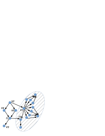
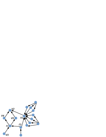
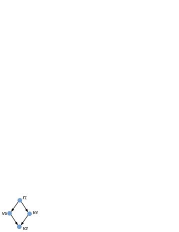
Figure 1: In Figure 1, the dependency scores of the vertices in the hachured part of the graph (and also $v_{3}$) on $r_{1}$ is 0. The graph of Figure 1 presents the reverse graph of the graph of Figure 1. Figure 1 shows how $\mathcal{RV}(r_{1})$ is computed.

Definition 4.1

Let $G$ be a directed graph and $r,v\in V(G)$. We say $r$ is reachable from $v$ if there is a (directed) path from $v$ to $r$. The set of vertices that $r$ is reachable from them is denoted by $RV(r)$.

Proposition 4.2

Let $G$ be a directed graph and $r\in V(G)$. If out degree of $r$ is $0$, $BC(r)$ is $0$, too. Otherwise, we have:

$$BC(r)=\sum_{v\in RV(r)}\delta_{v\bullet}(r).$$ (5)

Proof 4.3

If out degree of $r$ is $0$, there is no shortest path in the graph that leaves $r$, as a result, $BC(r)$ is $0$. To prove that Equation 5 holds, we need to prove that for any $w\in V(G)\setminus RV(r)$, dependency score of $w$ on $r$ is $0$. Obviously, this holds, because there is no path from $w$ to $r$ and as a result, no shortest path starting from $w$ can pass over $r$.

Proposition 4.2 suggests that for computing betweenness score of $r$, we first check whether out degree of $r$ is greater than $0$ and if so, we compute $RV(r)$. Betweenness score of $r$ is exactly computed using Equation 5.

If $RV(r)$ is already known, this procedure can significantly improve computation of betweenness centrality of $r$. The reason is that, as our experiments show, in real-world directed networks $RV(r)$ is usually significantly smaller than $V(G)$. However, computing $RV(r)$ can be computationally expensive as in the worst case, it requires the same amount of time as computing betweenness score of $r$. This motivates us to try to define a set $\mathcal{RV}(r)$ that satisfies the following properties: (i) $RV(r)\subseteq\mathcal{RV}(r)$ and (ii) $\mathcal{RV}(r)$ can be computed effectively in a time much faster than computing $BC(r)$. Condition (i) implies that each vertex $v\in V(G)$ whose dependency score on $r$ is greater than $0$, belongs to $\mathcal{RV}(r)$ and as a result, $BC(r)=\sum_{v\in\mathcal{RV}(r)}\delta_{v\bullet}(r).$ In the following, we present a definition of $\mathcal{RV}(r)$ and a simple and efficient algorithm to compute it.

Definition 4.4

Let $G$ be a directed graph. Reverse graph of $G$, denoted by $R(G)$, is a directed graph such that: (i) $V(R(G))=V(G)$, and (ii) $(u,v)\in E(R(G))$ if and only if $(v,u)\in E(G)$.

For example, the graph of Figure 1 presents the reverse graph of the graph of Figure 1.

Definition 4.5

Let $G$ be a directed graph and $r\in V(G)$. We define $\mathcal{RV}(G)$ as the set that contains any vertex $v$ such that there is a path from $r$ to $v$ in $R(G)$.

Proposition 4.6

Let $G$ be a directed graph and $r\in V(G)$. We have: $RV(r)=\mathcal{RV}(r)$.

Proof 4.7

The proof is straight-forward from the definitions of $RV(r)$ and $\mathcal{RV}(r)$. For each $v\in V(G)$, if $v\in RV(r)$, then there is a path from $v$ to $r$ and as a result, there is a path from $r$ to $v$ in $R(G)$. Hence, $v\in\mathcal{RV}(r)$ and therefore, $RV(r)\subseteq\mathcal{RV}(r)$. In a similar way, we can show that $\mathcal{RV}(r)\subseteq RV(r)$. Therefore, we have: $RV(r)=\mathcal{RV}(r)$.

An advantage of the above definition of $\mathcal{RV}(r)$ is that it can be efficiently computed as follows:

1. first, by flipping the direction of the edges of $G$, $R(G)$ is constructed.

2. then, if $G$ is weighted, the weights of the edges are ignored,

3. finally, a breadth first search (BFS) or a depth-first search (DFS) on $R(G)$ starting from $r$ is performed. All the vertices that are met during the BFS (or DFS), except $r$, are added to $\mathcal{RV}(r)$.

In fact, while in $RV(r)$ we require to solve the multi-source shortest path problem (MSSP), in $\mathcal{RV}(r)$ this is reduced to the single-source shortest path problem (SSSP), which can be addressed much faster. Figure 1 shows an example of this procedure, where in order to compute $\mathcal{RV}(r_{1})$, we first generate $R(G)$ (Figure 1) and then, we run a BFS (or DFS) starting from $r_{1}$ (Figure 1). The set of vertices that are met during the traversal except $r_{1}$, i.e., vertices $v_{2}$, $v_{4}$ and $v_{5}$, form $\mathcal{RV}(r_{1})$.

For a vertex $r\in V(G)$, each of the steps of the procedure of computing $\mathcal{RV}(r)$, for both unweighted graphs and weighted graphs, can be computed in $\Theta(|E(G)|)$ time. Hence, time complexity of the procedure of computing $\mathcal{RV}(r)$ for both unweighted graphs and weighted graphs is $\Theta(|E(G)|)$. Therefore, $\mathcal{RV}(r)$ can be computed in a time much faster than computing betweenness score f $r$. Furthermore, Proposition 4.6 says that $\mathcal{RV}(r)$ contains all the members of $RV(r)$. These two imply that both of the afore-mentioned conditions are satisfied.

4.2 The exact algorithm

In this section, using the notions and definitions presented in Section 4.1, we propose an effective algorithm to compute exact betweenness score of a given vertex $r$ in a directed graph $G$.

Algorithm 1 presents the high level pseudo code of the E-BCD algorithm proposed for computing exact betweenness score of $r$ in $G$. After checking whether or not out degree of $r$ is $0$, the algorithm follows two main steps: (i) computing $\mathcal{RV}(G)$ (Lines 7-12 of Algorithm 1), where we use the procedure described in Section 4.1 to compute $\mathcal{RV}(r)$; and (ii) computing $BC(r)$ (Lines 13-18 of Algorithm 1), where for each vertex $v\in\mathcal{RV}(r)$, we form the SPD rooted at $v$ and compute the dependency score of $v$ on the other vertices and add the value of $\delta_{v\bullet}(r)$ to the betweenness score of $r$. Note that if $G$ is weighted, while in the first step the weights of its edges are ignored, in the second step and during forming SPDs and computing dependency scores, we take the weights into account.

Note also that in Algorithm 1, after computing $\mathcal{RV}(r)$, techniques proposed to improve exact betweenness centrality computation, such compression and shattering [14], can be used to improve the efficiency of the second step. This means the algorithm proposed here is orthogonal to the techniques such as shattering and compression and therefore, they can be merged.

Complexity analysis

On the one hand, as mentioned before, time complexity of the first step is $\Theta(|E(G)|)$. On the other hand, time complexity of each iteration in Lines 15-18 is $\Theta(|E(G)|)$ for unweighted graphs and $\Theta(|E(G)|+|V(G)|\log|V(G)|)$ for weighted graphs with positive weights. As a result, time complexity of E-BCD is $\Theta(|\mathcal{RV}(G)|\cdot|E(G)|)$ for unweighted graphs and $\Theta(|\mathcal{RV}(G)|\cdot|E(G)|+|\mathcal{RV}(G)|\cdot|V(G)|\log|V(G)|)$ for weighted graphs with positive weights. Since most of vertices in real-world networks have a small reachable set (see Section 5), this time complexity improves time complexity of Brandes’ algorithm [4].

Algorithm 1 High level pseudo code of the algorithm of computing exact betweenness centrality in directed graphs.

1:  E-BCD

2:  Input. A directed network $G$ and a vertex $r\in V(G)$.

3:  Output. Betweenness score of $r$.

4:  if out degree of $r$ is $0$ then

5:     return  $0$.

6:  end if

7:  {Compute $\mathcal{RV}(r)$:}

8:  $\mathcal{RV}(r)\leftarrow\emptyset$.

9:  $R(G)\leftarrow$ compute the reverse graph of $G$.

10:  If $G$ is weighted, ignore the weights of the edges of $R(G)$.

11:  Perform a BFS or DFS on $R(G)$ starting from $r$.

12:  Add to $\mathcal{RV}(r)$ all the visited vertices, except $r$.

13:  {Compute $BC(r)$:}

14:  $bc\leftarrow 0$.

15:  for all vertices $v\in\mathcal{RV}(G)$ do

16:     Form the SPD rooted at $v$ and compute the dependency scores of $v$ on the other vertices.

17:     $bc\leftarrow bc+\delta_{v\bullet}(r)$.

18:  end for

19:  return  $bc$.

E-BCD can be simply revised to compute betweenness scores of all vertices in a set $R=\{r_{1},\ldots,r_{l}\}$ ($l$ is the cardinality of $R$). Let $\mathcal{D}$ be $\cup_{r_{i}\in R}\mathcal{RV}(r_{i})$. After forming the SPD rooted at each vertex in $\mathcal{D}$, we can easily compute betweenness scores of all the vertices in $R$. Someone may wonder for what sizes of $R$ E-BCD yields a better algorithm than Brandes’ algorithm. Assume that forming the SPD rooted at a vertex $v_{i}$ and computing dependency scores of $v_{i}$ on other vertices takes the same time $f$ as finding $\mathcal{RV}(v_{i})$. While in practice the former takes usually more time than the latter (as it needs to traverse the SPD twice), this assumption can be particularly valid in theory for unweighted graphs, as both of these two operations have the same asymptotic time complexity. E-BCD spends $l\cdot f+|\mathcal{D}|\cdot f=(l+|\mathcal{D}|)\cdot f$ time to compute the scores. Brandes’ algorithm on the other hand spends $|V(G)|\cdot f$ time. This means if $l<|V(G)|-|\mathcal{D}|$, E-BCD outperforms Brandes’ algorithm, otherwise, Brandes’ algorithm will have a smaller time complexity.

4.3 The approximate algorithm

For a vertex $r\in V(G)$, $\mathcal{RV}(r)$ is always smaller than $|V(G)|$ and as our experiments (reported in Section 5) show, the difference is usually significant. Therefore, E-BCD is usually significantly more efficient than the existing exact algorithms such as Brandes’s algorithm [4]. However, in some cases, the size of $\mathcal{RV}(r)$ can be large (see again Section 5). To make the algorithm tractable for the cases where $\mathcal{RV}(r)$ is large, in this section we propose a randomized algorithm that picks some elements of $\mathcal{RV}(r)$ uniformly at random and only processes these vertices.

Algorithm 2 shows the high level pseudo code of our randomized algorithm, called A-BCD. Similar to E-BCD, A-BCD first computes $\mathcal{RV}(r)$. Then, at each iteration $t$ ($1\leq t\leq T$), A-BCD picks a vertex $v$ from $\mathcal{RV}(r)$ uniformly at random, forms the SPD rooted at $v$ and computes $\delta_{v\bullet}(r)$. In the end, betweenness of $r$ is estimated as the sum of the computed dependency scores on $r$ multiply by $\frac{|\mathcal{RV}(r)|}{T}$.

Algorithm 2 High level pseudo code of the algorithm of computing approximate betweenness centrality in directed graphs.

1:  A-BCD

2:  Input. A network $G$, a vertex $r\in V(G)$ and the number of samples $T$.

3:  Output. Estimated betweenness score of $r$.

4:  if out degree of $r$ is $0$ then

5:     return  $0$.

6:  end if

7:  {Compute $\mathcal{RV}(r)$:}

8:  $\mathcal{RV}(r)\leftarrow\emptyset$.

9:  $R(G)\leftarrow$ compute the reverse graph of $G$.

10:  If $G$ is weighted, ignore the weights of the edges of $R(G)$.

11:  Perform a BFS or DFS on $R(G)$ starting from $r$.

12:  Add to $\mathcal{RV}(r)$ all visited vertices, except $r$.

13:  {Estimate $BC(r)$:}

14:  $bc\leftarrow 0$.

15:  for all $t=1$ to $T$  do

16:     Select a vertex $v_{t}\in\mathcal{RV}(r)$ uniformly at random.

17:     Form the SPD rooted at $v_{t}$ and compute dependency scores of $v_{t}$ on the other vertices.

18:     $bc\leftarrow bc+\frac{\delta_{v_{t}\bullet}(r)\cdot|\mathcal{RV}(r)|}{T}$.

19:  end for

20:  return  $bc$.

Complexity analysis

Similar to E-BCD, on the one hand, time complexity of the $\mathcal{RV}(r)$ computation step is $\Theta(|E(G)|)$. On the other hand, time complexity of each iteration in Lines 15-19 of Algorithm 2 is $\Theta(|E(G)|)$ for unweighted graphs and $\Theta(|E(G)|+|V(G)|\log|V(G)|)$ for weighted graphs with positive weights. As a result, time complexity of A-BCD is $\Theta(T\cdot|E(G)|)$ for unweighted graphs and $\Theta(T\cdot|E(G)|+T\cdot|V(G)|\log|V(G)|)$ for weighted graphs with positive weights, where $T$ is the number of iterations (samples).

Error bound

Using Hoeffding’s inequality [37], we can simply derive an error bound for the estimated value of betweenness score of $r$. First in Proportion 4.8, we prove that in Algorithm 2 the expected value of $bc$ is $BC(r)$. Then in Proportion 4.10, we provide an error bound for $bc$.

Proposition 4.8

In Algorithm 2, we have: $\mathbb{E}\left[bc\right]=BC(r)$.

Proof 4.9

For each $t$, $1\leq t\leq T$, we define random variable $bc_{t}$ as follows: $bc_{t}=\delta_{v_{t}\bullet}(r)\cdot|\mathcal{RV}(r)|$. We have:

$$\mathbb{E}\left[bc_{t}\right] =\sum_{v\in\mathcal{RV}(r)}\left(\frac{1}{|\mathcal{RV}(r)|}\cdot\delta_{v_{t}\bullet}(r)\cdot|\mathcal{RV}(r)|\right)=BC(r).$$

The random variable $bc$ is the average of $T$ independent random variables $bc_{t}$. Therefore, we have:

$$\mathbb{E}\left[bc\right]=\frac{\sum_{t=1}^{T}\mathbb{E}\left[bc_{t}\right]}{T}=\frac{T\cdot\mathbb{E}\left[bc_{t}\right]}{T}=BC(r).$$

Proposition 4.10

In Algorithm 2, let $K$ be the maximum dependency score that a vertex may have on $r$. For a given $\epsilon\in\mathbb{R}^{+}$, we have:

$$\mathbb{P}\left[\left|BC(r)-bc\right|>\epsilon\right]\leq 2\exp\left(-2T\cdot\left(\frac{\epsilon}{K\cdot|\mathcal{RV}(r)|}\right)^{2}\right).$$ (6)

Proof 4.11

The proof is done using Hoeffding’s inequality [37]. Let $X_{1},\ldots,X_{n}$ be independent random variables bounded by the interval $[a,b]$, i.e., $a\leq X_{i}\leq b$ ($1\leq i\leq n$). Let also $\bar{X}=\frac{1}{n}\left(X_{1}+\ldots+X_{n}\right)$. Hoeffding [37] showed that:

$$\mathbb{P}\left[\left|\mathbb{E}\left[\bar{X}\right]-\bar{X}\right|>\epsilon\right]\leq 2\exp\left(-2n\cdot\left(\frac{\epsilon}{b-a}\right)^{2}\right).$$ (7)

Similar to the proof of Proposition 4.8, for each $t$, $1\leq t\leq T$, we define random variable $bc_{t}$ as follows: $bc_{t}=\delta_{v_{t}\bullet}(r)\cdot|\mathcal{RV}(r)|$. Note that in Algorithm 2 vertices $v_{t}$ are chosen independently, as a result, random variables $bc_{t}$ are independent, too. Hence, we can use Hoeffding’s inequality, where $X_{i}$’s are $bc_{t}$’s, $\bar{X}$ is $bc$, $n$ is $T$, $a$ is $0$ and $b$ is $K\cdot|\mathcal{RV}(r)|$. Putting these values into Inequality 7 yields Inequality 6.

Inequality 6 says that for given values $\epsilon\in\mathbb{R}^{+}$ and $\delta\in(0,1)$, if $T$ is chosen such that

$$T\geq\frac{\ln\left(\frac{2}{\delta}\right)\cdot K^{2}\cdot|\mathcal{RV}(r)|^{2}}{2{\epsilon}^{2}},$$ (8)

then, Algorithm 2 estimates betweenness score of $r$ within an additive error $\epsilon$ with a probability at least $1-\delta$. The difference between Inequality 8 and the number of samples required by the methods that uniformly sample from the set of all vertices (e.g., [25]) is that in the later case, the lower bound on the number of samples is a function of $|V(G)|^{2}$, instead of $|\mathcal{RV}(r)|^{2}$. As mentioned earlier, for most of the vertices, $|\mathcal{RV}(r)|\ll|V(G)|$.

5 Experimental results

We perform extensive experiments on several real-world networks to assess the quantitative and qualitative behavior of our proposed exact and approximate algorithms. The experiments are done on an Intel processor clocked at 2.6 GHz with 16 GB main memory, running Ubuntu Linux 16.04 LTS. All the programs are compiled by the GNU C++ compiler 5.4.0 using optimization level 3.

We test the algorithms over several real-world datasets from different domains, including the amazon product co-purchasing network [38], the com-dblp co-authorship network [39], the com-amazon network [39] the p2p-Gnutella31 peer-to-peer network [40], the slashdot technology-related news network [41] and the soc-sign-epinions who-trust-whom online social network [41]. All the networks are treated as directed graphs. Table 1 summarizes specifications of our real-world networks.

Table 1: Summary of real-world datasets.

Dataset	# vertices	# edges
Amazon	262,111	1,234,877
Com-amazon	334,863	925,872
Com-dblp	317,080	1,049,866
Email-EuAll	224,832	340,795
P2p-Gnutella31	62,586	147,892
Slashdot	82,144	549,202
Soc-sign-epinions	131,828	841,372
Web-NotreDame	325,729	1,497,134

As mentioned before, for a directed graph $G$ and a vertex $r\in V(G)$, both of our proposed exact and approximate algorithms first compute $\mathcal{RV}(r)$, which can be done very effectively. Then, based on the size of $\mathcal{RV}(r)$, someone may decide to use either the exact algorithm or the approximate algorithm. Hence in our experiments, we follow the following procedure:

• first, compute $\mathcal{RV}(r)$,

• then, if $|\mathcal{RV}(r)|\leq\tau$, run E-BCD; otherwise, run A-BCD with $\tau$ as the number of samples.

We refer to this procedure as BCD. The value of $\tau$ depends on the amount of time someone wants to spend for computing betweenness centrality. In our experiments reported here, we set $\tau$ to 1000. We compare our method against the most efficient existing algorithm for approximating betweenness centrality, which is KADABRA [31].

For a vertex $r\in V(G)$, its empirical approximation error is defined as:

$$Error(v)=\frac{|App(v)-BC(v)|}{BC(v)}\times 100,$$ (9)

where $App(v)$ is the calculated approximate score.

5.1 Results

Table 2 reports the results of our first set of experiments. For KADABRA, we have set $\epsilon$ and $\delta$ to $0.01$ and $0.1$, respectively. Then from each dataset we choose $1000$ vertices uniformly at random and run BCD for any of these vertices. For the BCD algorithm, we report both ”Avg. time” and ”$\text{Avg. time}_{\mathcal{RV}}$”, where ”$\text{Avg. time}_{\mathcal{RV}}$” is the average of run times of computing $\mathcal{RV}$ and ”Avg. time” is the average of run times of the other parts of the algorithm. The average total running time of BCD is the sum of ”Avg. time” and ”$\text{Avg. time}_{\mathcal{RV}}$”. We also report ”Avg. error”, which is the average of empirical approximation errors (defined in Equation 9), and ”$\%$exact” that presents the percentage of the vertices for which BCD computes betweenness scores exactly, hence, their approximation error is $0$. We remind that if $|\mathcal{RV}|\geq 1000$, approximate BCD is used, otherwise, exact BCD is employed. As can be seen in the table, BCD estimates betweenness centrality of a single vertex much faster and with much less error. It is notable that in most cases, BCD computes the exact score within a tiny time, whereas KADABRA estimates the score with a large error within a much longer time.

Table 2: Empirical evaluation of BCD against KADABRA for $1000$ randomly chosen vertices. Values of $\delta$ and $\epsilon$ are $0.1$ and $0.01$, respectively. All the reported times are in seconds. The number of samples in A-BCD is $1000$. ’$\%$exact’ presents the percentage of the vertices for which betweenness scores are computed exactly by BCD-E and ’Avg. $\text{time}_{\mathcal{RV}}$’ presents the average time to compute reachable vertices.

Dataset	Randomly chosen vertices		KADABRA			BCD
	Avg. $|\mathcal{RV}(r)|$	Avg. $\frac{|\mathcal{RV}(r)|}{|V(G)|}$	$\#$samples	Time	Error ($\%$)	$\%$exact	Avg. time	Avg. $\text{time}_{\mathcal{RV}}$	Avg. error ($\%$)
Amazon	3453.714	0.013	16739	19.14	100	92.857	0.673	0.331	0.018
Com-amazon	74.533	0.0002	15036	27.70	100	100	0.512	0.367	0
Com-dblp	24635.923	0.077	17873	26.14	100	69.230	2.14	0.322	2.678
Email-EuAll	13652.785	0.0607	17066	16.01	100	64.285	0.964	0.083	0.995
P2p-Gnutella31	7246.071	0.115	16401	6.88	100	57.142	2.221	0.046	5.854
Slashdot0902	6662.866	0.0811	17421	7.95	100	80	0.995	0.130	6.279
Soc-sign-epinions	14567.875	0.110	19099	11.28	100	62.5	1.789	0.150	9.234
Web-NotreDame	431.714	0.001	19908	27.29	100	85.714	0.852	0.240	0.041

Table 3: Empirical evaluation of BCD against KADABRA for some of randomly chosen vertices. Values of $\delta$ and $\epsilon$ are $0.1$ and $0.01$, respectively. All the reported times are in seconds. The number of samples in A-BCD is $1000$.

Dataset	Randomly chosen vertices				KADABRA			BCD
	$r$	$BC(r)$	$|\mathcal{RV}(r)|$	$\frac{|\mathcal{RV}(r)|}{|V(G)|}$	$\#$samples	Time	Error ($\%$)	E/A	Time	$\text{Time}_{\mathcal{RV}}$	Error ($\%$)
Amazon	13645	19613.1	47187	0.1800	16739	19.14	100	A	2.60	0.26	0.26
	91289	87523.6	150	0.0005			100	E	0.67	0.29	0
	17054	35752.6	533	0.0020			100	E	1.26	0.29	0
	231249	10449.4	4	0.00001			100	E	0.11	0.30	0
	246486	1837.58	34	0.0001			100	E	0.17	0.30	0
Com-amazon	202389	1486.8	13	0.00003	15036	27.70	100	E	0.14	0.27	0
	263212	364	3	0.000008			100	E	0.12	0.27	0
	81097	11	14	0.00004			100	E	0.15	0.27	0
	13732	1701.51	616	0.0018			100	E	1.41	0.28	0
	29825	139	15	0.00004			100	E	0.15	0.27	0
Com-dblp	4456	10153	2092	0.0065	17873	26.14	100	A	5.74	0.26	1.10
	278950	34326.5	11	0.00003			100	E	0.13	0.27	0
	244680	232994	22	0.00006			100	E	0.21	0.27	0
	21141	1957.93	73	0.0002			100	E	0.48	0.27	0
	129908	303543	41	0.0001			100	E	0.53	0.29	0
Email-EuAll	25362	1869.16	2	0.000008	17066	16.01	100	E	0.03	0.08	0
	16682	2269.29	64	0.0002			100	E	0.14	0.08	0
	8796	241434	21181	0.0942			100	A	1.88	0.07	1.72
	50365	3	2	0.000008			100	E	0.03	0.07	0
	2139	503650	111674	0.4966			100	A	1.78	0.08	3.59
P2p-Gnutella31	46263	12655.2	2	0.00003	16401	6.88	100	E	0.03	0.04	0
	34547	3538.79	173	0.0027			100	E	0.95	0.04	0
	54609	27824.9	3	0.00004			100	E	0.03	0.04	0
	37518	6175.2	24141	0.3857			100	A	2.44	0.06	11.31
	9781	4582130	3	0.00004			100	E	0.02	0.04	0
Slashdot0902	20825	15940.9	21	0.0002	17421	7.95	100	E	0.17	0.16	0
	47806	15891.7	3	0.00003			100	E	0.06	0.15	0
	48251	21744	3	0.00003			100	E	0.05	0.15	0
	20969	43067	369	0.0044			100	E	2.30	0.17	0
	57099	6165.01	2	0.00002			100	E	0.05	0.15	0
Soc-sign-epinions	2740	2352.43	36393	0.2760	19099	11.28	100	A	4.57	0.17	55.34
	24080	9198.78	2621	0.0198			100	A	4.60	0.15	18.48
	38349	75201.9	35	0.0002			100	E	0.24	0.14	0
	82156	8802	34	0.0002			100	E	0.19	0.14	0
	38266	8052	3	0.00002			100	E	0.04	0.14	0
Web-NotreDame	21026	140	9	0.00002	19908	27.29	100	E	0.08	0.25	0
	133847	9003.53	797	0.0024			100	E	1.84	0.25	0
	307622	4212.33	44	0.0001			100	E	0.18	0.25	0
	176211	2157.42	30	0.00009			100	E	0.14	0.25	0
	307134	3079.5	123	0.0003			100	E	0.35	0.25	0

In order to investigate the behavior of the algorithms more deeply, over each dataset we choose $5$ vertices at random and report their results in Table 3. This table has a column, called ”A/E”, where ”E” means that the computed score by BCD is exact (hence, the approximation error is $0$) and ”A” means that $\mathcal{RV}$ is larger than $1000$, therefore approximate BCD has been employed.

As can be seen in Table 3, for most of the randomly picked up vertices, $\mathcal{RV}$ is very small and it can be computed very efficiently. This gives exact results in a very short time, less than $3$ seconds in total. In all these cases, while KADABRA spends considerably more time, since it estimates that the normalized betweenness scores are less than the error bound $\epsilon$, it simply estimates them as $0$. Therefore, its empirical approximation error becomes $100\%$. The randomly picked up vertices belong to the different ranges of betweenness scores, including high, medium and low.

After observing these experimental results, someone may be interested in the following questions:

• The accuracy of KADABRA depends on the values of $\epsilon$ and $\delta$. Can changing (increasing or decreasing) their values improve the performance of KADABRA and make it be comparable to BCD?

• KADABRA is more efficient for the vertices that have the highest betweenness scores and since most of the randomly chosen vertices do not have a very high betweenness score, compared to EBC, KADABRA does not show a good performance. What is the efficiency of BCD, compared to KADABRA, for the vertices that have the highest betweenness scores?

• In the experiments reported in Table 3, BCD is used to estimate betweenness score of only one vertex. However, in practice it might be required to estimate betweenness scores of a given set of vertices. How efficient is BCD in this setting?

In the rest of this section, we answer these questions.

Table 4: Empirical evaluation of KADABRA for $\delta=0.1$, $\epsilon=0.005$ and $0.05$.

Dataset	Vertex $r$	KADABRA ($\epsilon=0.005$)			KADABRA ($\epsilon=0.05$)
		$\#$samples	Time	Error ($\%$)	$\#$samples	Time	Error ($\%$)
Amazon	13645	47330	53.98	100	1615	3.648	100
	91289			100			100
	17054			100			100
	231249			100			100
	246486			100			100
Com-amazon	202389	42207	58.76	100	1390	4.36	100
	263212			100			100
	81097			100			100
	13732			100			100
	29825			100			100
Com-dblp	4456	50667	77.40	100	1627	4.15	100
	278950			100			100
	244680			100			100
	21141			100			100
	129908			100			100
Email-EuAll	25362	48079	43.43	100	1390	2.28	100
	16682			100			100
	8796			100			100
	50365			100			100
	2139			100			100
P2p-Gnutella31	46263	47631	18.12	100	1445	0.81	100
	34547			100			100
	54609			568.32			100
	37518			100			100
	9781			6.52			100
Slashdot0902	20825	50776	22.38	100	1542	0.94	100
	47806			100			100
	48251			100			100
	20969			100			100
	57099			100			100
Soc-sign-epinions	2740	53667	30.54	100	1479	1.90	100
	24080			100			100
	38349			100			100
	82156			100			100
	38266			100			100
Web-NotreDame	21026	51015	73.92	100	1935	2.21	100
	133847			100			100
	307622			100			100
	176211			100			100
	307134			100			100

Table 5: Empirical evaluation of BCD against KADABRA-TOP-1 for vertices with the highest betweenness scores. The value of $\delta$ is 0.1. All the reported times are in seconds. The number of samples in A-BCD is $1000$.

Dataset	Vertex with the highest BC				KADABRA-TOP-1				BCD
	$r$	$BC(r)$	$|\mathcal{RV}(r)|$	$\frac{|\mathcal{RV}(r)|}{|V(G)|}$	$\epsilon$	$\#$samples	Time	Error ($\%$)	Time	$\text{Time}_{\mathcal{RV}}$	Error ($\%$)
Amazon	2804	16066000	162707	0.6207	0.01	16181	0.26	-	2.38	0.29	1.35
					0.005	45320	0.56	71.69
					0.0005	1459502	16.65	3.01
Com-amazon	28081	378550	3812	0.0113	0.01	14619	0.14	-	2.31	0.28	0.52
					0.005	40590	0.21	-
					0.0005	1249908	3.86	28.90
Com-dblp	49124	24821300	70561	0.2225	0.01	17303	0.64	17.04	6.27	0.27	9.77
					0.005	48411	1.62	7.96
					0.0005	1581635	54.11	6.79
Email-EuAll	2387	15943100	102596	0.4563	0.01	16588	0.10	33.79	1.76	0.08	3.37
					0.005	46123	0.17	17.50
					0.0005	1471932	3.87	4.04
P2p-Gnutella31	9781	4580850	36141	0.5774	0.01	13618	0.32	57.61	1.78	0.04	2.59
					0.005	40909	1.00	6.51
					0.0005	1515822	38.31	0.32
Slashdot0902	18238	8531850	19153	0.2331	0.01	16962	0.99	11.96	3.90	0.10	3.37
					0.005	44847	2.52	5.87
					0.0005	1718486	103.89	0.16
Soc-sign-epinions	27463	26116100	9880	0.0749	0.01	18601	1.10	2.25	5.43	0.12	2.30
					0.005	51502	2.97	0.23
					0.0005	2398143	143.92	1.61
Web-NotreDame	7137	323101000	233965	0.7182	0.01	19448	0.18	1.30	2.71	0.235	0.26
					0.005	49456	0.30	7.56
					0.0005	779273	3.93	2.22

Q1

To answer Q1, first we fix $\delta$ to $0.1$ and run KADABRA with $\epsilon=0.005$ (i.e., with a lower value) and $\epsilon=0.05$ (i.e., with a higher value). The results are reported in Table 4. In these two settings, most of the scores estimated by KADABRA are still $0$. There are only two exceptions where, however, the approximation error is high. For $\epsilon=0.005$, the running time of KADABRA is considerably more than its running time for $\epsilon=0.01$ and as a result, the running time of BCD. However, paying this extra cost does not improve its accuracy, with respect to BCD. Increasing $\epsilon$ to $0.05$, reduces running time of KADABRA and makes it comparable to the running time of BCD. However, BCD shows a much better accuracy.

Then, we fix $\epsilon$ to $0.01$ and run KADABRA with $\delta=0.05$ (i.e., with a lower value) and $\delta=0.15$ (i.e., with a higher value). In these cases, we do not observe meaningful changes in the behavior (running time and accuracy) of KADABRA. We may only state that in the case of $\delta=0.15$, the algorithm works slightly faster. As a result, it seems KADABRA is less sensitive to the value of $\delta$ than to the value of $\epsilon$. Due to the high similarity of the results obtained in these two cases to the results of Table 3, we do not report them.

Q2

To answer Q2, over each dataset we examine the algorithms for the vertex that has the highest betweenness score. The results are reported in Table 5. KADABRA can be optimized to estimate betweenness centrality of only top $k$ vertices, where $k$ is an input parameter. In the experiments of this part, we use this optimized version of KADABRA with $k=1$ and refer to it as KADABRA-TOP-1. In KADABRA-TOP-1, we consider three values for $\epsilon$: $0.01$, $0.005$ and $0.0005$ and in all the cases, we set $\delta$ to $0.1$. Similar to the other experiments, we run BCD with $\tau=1000$. In all the experiments of this part, the size of $\mathcal{RV}$ becomes larger than $1000$, hence, the scores computed by BCD are approximate scores. In Table 5, in three cases the error of KADABRA-TOP-1 is not reported. The reason is that in these cases the vertex $r$ that has the highest betweenness score, is not among the vertices considered by KADABRA-TOP-1 as a top-score vertex. Hence, KADABRA-TOP-1 does not report any value for it.

In this setting, none of the algorithms outperforms the other one in all the cases. More precisely, while for some values of $\epsilon$ KADABRA-TOP-1 has a better accuracy as well as a higher running time, in some other cases the story is in the other way. Nevertheless, we can investigate the datasets one by one. Over amazon, for all values of $\epsilon$, BCD has a better approximation error than KADABRA-TOP-1. In particular, for $\epsilon=0.0005$, KADABRA-TOP-1 takes much more time but produces a less accurate output. Hence, we can argue that over amazon BCD outperforms KADABRA-TOP-1. The same holds for com-amazon, email-EuAll and web-NotreDame and over all these datasets, BCD outperforms KADABRA-TOP-1. Over com-dblp, for $\epsilon=0.005$, KADABRA-TOP-1 outperforms BCD in terms of both accuracy and running time. This also happens over soc-sign-epinions for $\epsilon=0.01$ and $0.005$. Hence, someone may argue that over these two datasets KADABRA-TOP-1 outperforms BCD. Over p2p-Gnutella31 and slashdot0902, on the one hand for $\epsilon=0.01$ and $0.005$, BCD shows a better accuracy, however, it is slightly slower. On the other hand, for $\epsilon=0.0005$, KADABRA-TOP-1 shows a better accuracy, however, it takes much more time. Altogether, we can say that for estimating betweenness scores of the vertices that have the highest scores, in most of the datasets BCD works better than KADABRA-TOP-1.

Table 6: Empirical evaluation of estimating betweenness scores of a set of vertices. All the reported times are in seconds. The number of samples in A-BCD is $1000$.

Dataset	Set size	Error ($\%$)			Time	$\text{Time}_{\mathcal{RV}}$	$\mathcal{RV}$ size
		Avg.	Max.	Min.			Avg.	Max.	Min.
Amazon	5	1.47	7.10	0	4.81	1.44	9581.6	47187	4
	10	0.73	7.10	0	7.42	3.21	4818.4	47187	1
	15	0.88	7.10	0	9.74	4.98	3497.798	47187	1
Com-amazon	5	0	0	0	1.98	1.36	132.2	616	3
	10	0	0	0	4.92	3.43	91.2	616	2
	15	0	0	0	7.07	5.48	65.93	616	1
Com-dblp	5	0.22	1.10	0	7.09	1.36	447.8	2092	11
	10	3.47	19.45	0	20.71	3.08	24483.6	227218	1
	15	2.32	19.45	0	28.81	4.92	21351.33	227218	1
Email-EuAll	5	1.06	3.59	0	3.86	0.38	26584.6	111674	2
	10	1.39	7.95	0	9.76	0.78	19020.9	111674	2
	15	0.93	7.95	0	13.52	1.27	12742.8	111674	2
P2p-Gnutella31	5	2.26	11.31	0	3.47	0.22	4864.2	24141	2
	10	7.26	39.17	0	23.09	0.46	5493.6	24141	2
	15	6.79	39.17	0	33.27	0.72	8637.73	28122	2
Slashdot0902	5	0	0	0	2.62	0.78	79.6	369	2
	10	5.04	50.48	0	11.37	1.38	3784.3	26802	1
	15	4.92	50.48	0	14.93	1.99	6662.86	62089	1
Soc-sign-epinions	5	13.37	48.37	0	9.64	0.74	7817.2	36393	3
	10	9.68	48.37	0	17.71	1.52	20302.7	109520	1
	15	9.38	48.37	0	28.46	2.28	15538.86	109520	1
Web-NotreDame	5	0	0	0	2.58	1.25	200.6	797	9
	10	0	0	0	6.89	2.44	231.5	1092	9
	15	0.03	0.30	0	13.16	3.62	414.46	2610	1

Q3

To answer Q3, we select a random set of vertices and run BCD for each vertex in the set. The results are reported in Table 6, where the set contains 5, 10 or 15 vertices. Over all the datasets and for each set of vertices, we report the average, maximum and minimum errors of the vertices. For all the datasets, minimum error is always 0. In Table 6, ”$\text{Time}_{\mathcal{RV}}$” is the total time of computing $\mathcal{RV}$ of all the vertices in the set and ”Time” is the total time of the other steps of computing betweenness scores of all the vertices in the set. Therefore, the total running time of BCD for a given dataset and a given set is the sum of ”Time” and ”$\text{Time}_{\mathcal{RV}}$”. Comparing the results presented in Table 6 with the results presented in Table 4 reveals that for estimating betweenness scores of a set of vertices, BCD considerably outperforms KADABRA (where $\epsilon$ is $0.005$). While in most cases the total running time of BCD is less than the running time of KADABRA (even when the size of the set is 15), BCD gives much more accurate results. Note that even when in KADABRA $\epsilon$ is set to 0.01, in many cases BCD is faster than KADABRA. In particular, over datasets such as amazon, com-amazon, email-EuAll and web-NotreDame, even for the sets of size 15, BCD is faster than KADABRA and it always produces much more accurate results.

5.2 Discussion

Our extensive experiments reveal that BCD usually significantly outperforms KADABRA. This is due to the huge pruning that $\mathcal{RV}$ applies to the set of source vertices that are used to form SPDs and compute dependency scores. Note that in all the cases, $\mathcal{RV}$ is computed very efficiently, hence, it does not impose a considerable load on the algorithm. In the case of estimating betweenness score of the vertex with the highest betweenness score, over two datasets we may argue that KADABRA outperforms BCD. This has two reasons. On the one hand, in these cases the ratio $\frac{\mathcal{RV}(r)}{|V(G)|}$ is large, as a result, many SPDs are computed by BCD. On the other hand, the SPDs contain many vertices of the graph, as a result, their computation is expensive.

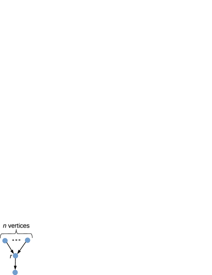
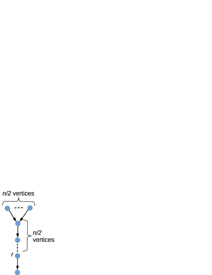
Figure 2: Using BCD, in the graph of Figure 2, $BC(r)$ is computed in $O(n)$ time; whereas in the graph of Figure 2, $BC(r)$ is computed in $O(n^{2})$ time.

In the end, it is worth mentioning that while the size of $\mathcal{RV}$ is an important factor on the efficiency of our algorithm, it is not the sole factor. For example, both graphs of Figure 2 have $n+2$ vertices, the size of $\mathcal{RV}(r)$ in Figure 2 is $n$ and the size of $\mathcal{RV}(r)$ in Figure 2 is $\frac{n}{2}$. However, in Figure 2 each SPD is computed and processed in $O(1)$ time, whereas in Figure 2 each SPD is computed and processed in $O(n)$ time. Therefore, while in Figure 2 $BC(r)$ is computed in $O(n)$ time, in Figure 2 it is computed in $O(n^{2})$ time.

6 Conclusion

In this paper, we studied the problem of computing betweenness score in large directed graphs. First, given a directed network $G$ and a vertex $r\in V(G)$, we proposed an exact algorithm to compute betweenness score of $r$. Our algorithm first computes a set $\mathcal{RV}(r)$, which is used to prune a huge amount of computations that do not contribute to the betweenness score of $r$. Time complexity of our exact algorithm is respectively $\Theta(|\mathcal{RV}(r)|\cdot|E(G)|)$ and $\Theta(|\mathcal{RV}(r)|\cdot|E(G)|+|\mathcal{RV}(r)|\cdot|V(G)|\log|V(G)|)$ for unweighted graphs and weighted graphs with positive weights. Then, for the cases where $\mathcal{RV}(r)$ is large, we presented a simple randomized algorithm that samples from $\mathcal{RV}(r)$ and performs computations for only the sampled elements. Finally, we performed extensive experiments over several real-world datasets from different domains for several randomly chosen vertices as well as for the vertices with the highest betweenness scores. Our experiments revealed that for estimating betweenness score of a single vertex, our algorithm considerably outperforms the most efficient existing randomized algorithms, in terms of both running time and accuracy. They also showed that our algorithm improves the existing algorithms when someone is interested in computing betweenness values of the vertices in a set whose cardinality is very small ($15$ for the analyzed graphs).

Acknowledgement

This work has been supported in part by the ANR project IDOLE.

References

- [1] Newman MEJ. The structure and function of complex networks. SIAM REVIEW, 2003. 45:167–256. doi:10.1137/S003614450342480.
- [2] Freeman LC. A set of measures of centrality based upon betweenness, Sociometry. Social Networks, 1977. 40:35–41. doi:10.2307/3033543.
- [3] Girvan M, Newman MEJ. Community structure in social and biological networks. Natl. Acad. Sci. USA, 2002. 99:7821–7826. doi:10.1073/pnas.122653799.
- [4] Brandes U. A faster algorithm for betweenness centrality. Journal of Mathematical Sociology, 2001. 25(2):163–177. doi:10.1080/0022250X.2001.9990249.
- [5] Wang Y, Di Z, Fan Y. Identifying and Characterizing Nodes Important to Community Structure Using the Spectrum of the Graph. PLoS ONE, 2011. 6(11):e27418. doi:10.1371/journal.pone.0027418.
- [6] Agarwal M, Singh RR, Chaudhary S, Iyengar SRS. An Efficient Estimation of a Node’s Betweenness. In: Mangioni G, Simini F, Uzzo SM, Wang D (eds.), Complex Networks VI - Proceedings of the 6th Workshop on Complex Networks CompleNet 2015, New York City, USA, March 25-27, 2015, volume 597 of Studies in Computational Intelligence. Springer. ISBN 978-3-319-16111-2, 2015 pp. 111–121. 10.1007/978-3-319-16112-9_11.
- [7] Agarwal M, Singh RR, Chaudhary S, Iyengar S. Betweenness Ordering Problem : An Efficient Non-Uniform Sampling Technique for Large Graphs. CoRR, 2014. abs/1409.6470. URL http://arxiv.org/abs/1409.6470.
- [8] Stergiopoulos G, Kotzanikolaou P, Theocharidou M, Gritzalis D. Risk mitigation strategies for critical infrastructures based on graph centrality analysis. International Journal of Critical Infrastructure Protection, 2015. 10:34 – 44. doi:10.1016/j.ijcip.2015.05.003.
- [9] Chehreghani MH. An Efficient Algorithm for Approximate Betweenness Centrality Computation. Comput. J., 2014. 57(9):1371–1382. 10.1093/comjnl/bxu003.
- [10] Malighetti G, Martini G, Paleari S, Redondi R. The Impacts of Airport Centrality in the EU Network and Inter- Airport Competition on Airport Efficiency. MPRA Paper 17673, University Library of Munich, Germany, 2009. URL https://ideas.repec.org/p/pra/mprapa/17673.html.
- [11] Bergamini E, Crescenzi P, D’Angelo G, Meyerhenke H, Severini L, Velaj Y. Improving the Betweenness Centrality of a Node by Adding Links. ACM Journal of Experimental Algorithmics, 2018. 23. URL https://dl.acm.org/citation.cfm?id=3166071.
- [12] Riondato M, Kornaropoulos EM. Fast approximation of betweenness centrality through sampling. Data Mining and Knowledge Discovery, 2016. 30(2):438–475. doi:10.1007/s10618-015-0423-0.
- [13] Chehreghani MH, Bifet A, Abdessalem T. Efficient Exact and Approximate Algorithms for Computing Betweenness Centrality in Directed Graphs. In: 22nd Pacific-Asia Conference on Knowledge Discovery and Data Mining, PAKDD. 2018 URL http://arxiv.org/abs/1708.08739.
- [14] Çatalyürek ÜV, Kaya K, Sariyüce AE, Saule E. Shattering and Compressing Networks for Betweenness Centrality. In: Proceedings of the 13th SIAM International Conference on Data Mining, May 2-4, 2013. Austin, Texas, USA. SIAM. ISBN 978-1-61197-262-7, 2013 pp. 686–694. 10.1137/1.9781611972832.76.
- [15] Holme P. Congestion and centrality in traffic flow on complex networks. Adv. Complex. Syst., 2003. 6(2):163–176. doi:10.1142/S0219525903000803.
- [16] Barthelemy M. Betweenness centrality in large complex networks. The Europ. Phys. J. B - Condensed Matter, 2004. 38(2):163–168. doi:10.1140/epjb/e2004-00111-4.
- [17] Barabasi AL, Albert R. Emergence of scaling in random networks. Science, 1999. 286:509–512.
- [18] Furno A, Faouzi NE, Sharma R, Zimeo E. Two-level clustering fast betweenness centrality computation for requirement-driven approximation. In: Nie J, Obradovic Z, Suzumura T, Ghosh R, Nambiar R, Wang C, Zang H, Baeza-Yates R, Hu X, Kepner J, Cuzzocrea A, Tang J, Toyoda M (eds.), 2017 IEEE International Conference on Big Data, BigData 2017, Boston, MA, USA, December 11-14, 2017. IEEE Computer Society, 2017 pp. 1289–1294. 10.1109/BigData.2017.8258057.
- [19] Everett M, Borgatti S. The centrality of groups and classes. Journal of Mathematical Sociology, 1999. 23(3):181–201.
- [20] Kolaczyk ED, Chua DB, Barthelemy M. Group-betweenness and co-betweenness: Inter-related notions of coalition centrality. Social Networks, 2009. 31(3):190–203. doi:10.1016/j.socnet.2009.02.003.
- [21] Chehreghani MH. Effective co-betweenness centrality computation. In: Seventh ACM International Conference on Web Search and Data Mining (WSDM). 2014 pp. 423–432. doi:10.1145/2556195.2556263.
- [22] Puzis R, Elovici Y, Dolev S. Fast algorithm for successive computation of group betweenness centrality. Phys. Rev. E, 2007. 76(5):056709. doi:10.1103/PhysRevE.76.056709.
- [23] Puzis R, Elovici Y, Dolev S. Finding the most prominent group in complex networks. AI Commun., 2007. 20(4):287–296.
- [24] Chehreghani MH, Bifet A, Abdessalem T. An In-depth Comparison of Group Betweenness Centrality Estimation Algorithms. In: Abe N, Liu H, Pu C, Hu X, Ahmed NK, Qiao M, Song Y, Kossmann D, Liu B, Lee K, Tang J, He J, Saltz JS (eds.), IEEE International Conference on Big Data, Big Data 2018, Seattle, WA, USA, December 10-13, 2018. IEEE, 2018 pp. 2104–2113. 10.1109/BigData.2018.8622133.
- [25] Brandes U, Pich C. Centrality estimation in large networks. Intl. Journal of Bifurcation and Chaos, 2007. 17(7):303–318.
- [26] Bader DA, Kintali S, Madduri K, Mihail M. Approximating betweenness centrality. In: Proceedings of 5th International Conference on Algorithms and Models for the Web-Graph (WAW). 2007 pp. 124–137. doi:10.1007/978-3-540-77004-6_10.
- [27] Geisberger R, Sanders P, Schultes D. Better approximation of betweenness centrality. In: Proceedings of the Tenth Workshop on Algorithm Engineering and Experiments (ALENEX). 2008 pp. 90–100.
- [28] Vapnik VN, Chervonenkis AY. On the uniform convergence of relative frequencies of events to their probabilities. Theory of Probab. and its Applications, 1971. 16(2):264–280.
- [29] Riondato M, Upfal E. ABRA: Approximating Betweenness Centrality in Static and Dynamic Graphs with Rademacher Averages. In: Proceedings of the 22Nd ACM SIGKDD International Conference on Knowledge Discovery and Data Mining, KDD ’16. ACM, New York, NY, USA. ISBN 978-1-4503-4232-2, 2016 pp. 1145–1154. 10.1145/2939672.2939770.
- [30] Shalev-Shwartz S, Ben-David S. Understanding Machine Learning: From Theory to Algorithms. Cambridge University Press, New York, NY, USA, 2014. ISBN 1107057132, 9781107057135.
- [31] Borassi M, Natale E. KADABRA is an ADaptive Algorithm for Betweenness via Random Approximation. In: Sankowski P, Zaroliagis CD (eds.), 24th Annual European Symposium on Algorithms, ESA 2016, August 22-24, 2016, Aarhus, Denmark, volume 57 of LIPIcs. Schloss Dagstuhl - Leibniz-Zentrum fuer Informatik. ISBN 978-3-95977-015-6, 2016 pp. 20:1–20:18. 10.4230/LIPIcs.ESA.2016.20.
- [32] Chehreghani MH, Abdessalem T, Bifet A. Metropolis-Hastings Algorithms for Estimating Betweenness Centrality. In: Herschel M, Galhardas H, Reinwald B, Fundulaki I, Binnig C, Kaoudi Z (eds.), Advances in Database Technology - 22nd International Conference on Extending Database Technology, EDBT 2019, Lisbon, Portugal, March 26-29, 2019. OpenProceedings.org, 2019 pp. 686–689. 10.5441/002/edbt.2019.87.
- [33] Lee MJ, Lee J, Park JY, Choi RH, Chung CW. QUBE: A quick algorithm for updating betweenness centrality. In: Proceedings of the 21st World Wide Web Conference (WWW). 2012 pp. 351–360.
- [34] Bergamini E, Meyerhenke H, Staudt C. Approximating Betweenness Centrality in Large Evolving Networks. In: Brandes U, Eppstein D (eds.), Proceedings of the Seventeenth Workshop on Algorithm Engineering and Experiments, ALENEX 2015, San Diego, CA, USA, January 5, 2015. SIAM. ISBN 978-1-61197-375-4, 2015 pp. 133–146. 10.1137/1.9781611973754.12.
- [35] Hayashi T, Akiba T, Yoshida Y. Fully Dynamic Betweenness Centrality Maintenance on Massive Networks. Proceedings of the VLDB Endowment (PVLDB), 2015. 9(2):48–59. URL http://www.vldb.org/pvldb/vol9/p48-hayashi.pdf.
- [36] Haghir Chehreghani M. Dynamical algorithms for data mining and machine learning over dynamic graphs. WIREs Data Mining and Knowledge Discovery, 2021. 11(2):e1393. doi:10.1002/widm.1393.
- [37] Hoeffding W. Probability Inequalities for Sums of Bounded Random Variables. Journal of the American Statistical Association, 1963. 58(301):13–30. URL http://www.jstor.org/stable/2282952?
- [38] Leskovec J, Adamic LA, Huberman BA. The dynamics of viral marketing. ACM Transactions on the Web (TWEB), 2007. 1(1). 10.1145/1232722.1232727.
- [39] Yang J, Leskovec J. Defining and Evaluating Network Communities Based on Ground-Truth. In: Zaki MJ, Siebes A, Yu JX, Goethals B, Webb GI, Wu X (eds.), 12th IEEE International Conference on Data Mining, ICDM 2012, Brussels, Belgium, December 10-13, 2012. IEEE Computer Society. ISBN 978-1-4673-4649-8, 2012 pp. 745–754. 10.1109/ICDM.2012.138.
- [40] Leskovec J, Kleinberg JM, Faloutsos C. Graph evolution: Densification and shrinking diameters. ACM Transactions on Knowledge Discovery from Data (TKDD), 2007. 1(1). 10.1145/1217299.1217301. URL http://doi.acm.org/10.1145/1217299.1217301.
- [41] Leskovec J, Huttenlocher DP, Kleinberg JM. Signed networks in social media. In: Mynatt ED, Schoner D, Fitzpatrick G, Hudson SE, Edwards WK, Rodden T (eds.), Proceedings of the 28th International Conference on Human Factors in Computing Systems, CHI 2010, Atlanta, Georgia, USA, April 10-15, 2010. ACM. ISBN 978-1-60558-929-9, 2010 pp. 1361–1370. 10.1145/1753326.1753532.