Beyond Outerplanarity

Abstract

We study straight-line drawings of graphs where the vertices are placed in convex position in the plane, i.e., convex drawings. We consider two families of graph classes with convex drawings: outer $k$-planar graphs, where each edge is crossed by at most $k$ other edges; and, outer $k$-quasi-planar graphs where no $k$ edges can mutually cross.

We show that the outer $k$-planar graphs are $\lfloor 3.5\sqrt{k}\rfloor$-degenerate, and consequently that every outer $k$-planar graph can be colored with $\lfloor 3.5\sqrt{k}\rfloor+1$ colors. We further show that every outer $k$-planar graph has a balanced vertex separator of size at most $2k+3$. For each fixed $k$, these small balanced separators allow us to test outer $k$-planarity in quasi-polynomial time, e.g., this implies that none of these recognition problems is NP-hard unless the Exponential Time Hypothesis fails. We also show that the class of outer $k$-quasi-planar graphs and the class of planar graphs are incomparable.

Finally, we restrict outer $k$-planar and outer $k$-quasi-planar drawings to full drawings (where no crossing appears on the boundary of the outer face) and to closed drawings (where the vertex sequence on the boundary of the outer face is a Hamiltonian cycle in the graph). For each $k$, we express closed outer $k$-planarity and closed outer $k$-quasi-planarity in extended monadic second-order logic. Due to a result of Wood and Telle (New York J. Math., 2007) every outer $k$-planar graph has treewidth at most $3k+11$. Thus, Courcelle’s theorem implies that closed outer $k$-planarity is linear time testable. We leverage this result to further show that full outer $k$-planarity can also be tested in linear time.

1 Introduction

A drawing of a graph maps each vertex to a distinct point in the plane, each edge to a Jordan curve connecting the points of its incident vertices but not containing the point of any other vertex, and two such Jordan curves have at most one common point. In the last few years, the focus in graph drawing has shifted from exploiting structural properties of planar graphs to addressing the question of how to produce well-structured (understandable) drawings in the presence of edge crossings, i.e., to the topic of beyond-planar graph classes. The primary approach here has been to define and study graph classes which allow some edge crossings, but restrict the crossings in various ways, such as, for example, restricting the total number of crossings [34] or even bundling the edges and restricting the number of crossings of bundles rather than of single edges [30, 18]. Two of the most commonly studied such graph classes are:

1. $k$-planar graphs, that is, the graphs that can be drawn so that each edge is crossed by at most $k$ other edges.

2. $k$-quasi-planar graphs, that is, the graphs that can be drawn so that no $k$ pairwise non-incident edges mutually cross.

Note that the $0$-planar graphs and $2$-quasi-planar graphs are precisely the planar graphs. Additionally, the $3$-quasi-planar graphs are simply called quasi-planar.

In this paper we restrict the two above families of graph classes by insisting on drawings where the vertices are in convex position and the edges are line segments. In other words, we apply the above two generalizations of planar graphs to outerplanar graphs, which yields the classes of outer $k$-planar graphs and outer $k$-quasi-planar graphs. (For an example, see Fig. 4, which shows a planar graph that is not outer quasi-planar, but removing any of its vertices makes it outer quasi-planar.) We consider balanced separators, treewidth, degeneracy (see Section 1.2 below), coloring, edge density, and recognition for these classes.

1.1 Related Work

Ringel [43] was the first to consider $k$-planar graphs; he showed that $1$-planar graphs are 7-colorable. Twenty years later, Ringel’s result was improved by Borodin [14], who showed that 1-planar graphs are in fact 6-colorable. This is tight since $K_{6}$ is 1-planar. Many additional results on 1-planarity can be found in a recent survey paper [36]. Generally, every $n$-vertex $k$-planar graph has at most $3.81n\sqrt{k}$ edges [2] and treewidth $O(\sqrt{kn})$ [25].

Outer $k$-planar graphs have been considered mostly for $k\in\{0,1,2\}$. Of course, the outer 0-planar graphs are the classic outerplanar graphs which are well-known to be 2-degenerate and to have treewidth at most 2. It was shown that essentially every graph property can be tested efficiently on outerplanar graphs [10]. Outer 1-planar graphs are a simple subclass of planar graphs and can be recognized in linear time [9, 31]. Full outer $2$-planar graphs, which form a subclass of outer $2$-planar graphs, can be recognized in linear time [32]. General outer $k$-planar graphs were considered by Binucci et al. [13], who showed (among other results) that, for every $k$, there is a 2-tree that is not outer $k$-planar. Wood and Telle [47] considered a slight generalization of outer $k$-planar graphs in their work and showed that these graphs have treewidth $O(k)$. Outer 1-planar graphs have been compared [15] with fan-crossing graphs (that is, graphs that have a drawing where each edge can only cross edges with a common endpoint) and fan-crossing free graphs (that is, graphs that have a drawing where no edge is crossed by two or more edges with a common endpoint). Fan-crossing and fan-crossing free are complementary properties, in the sense that a drawing is 1-planar if and only if it is fan-crossing and fan-crossing free. Brandenburg [15] showed that there are graphs that are simultaneously (outer-) fan-crossing and (outer-) fan-crossing free but not (outer-) 1-planar. Angelini et al. [7] studied the edge density of $k$-planar 2-layer layouts (where the vertices lie on two horizontal lines and every edge is a y-monotone curve). In order to admit such a layout, a graph must be bipartite, and the constraints on the placement of the vertices emphasize its bipartite structure.

The $k$-quasi-planar graphs have been studied extensively from the perspective of edge density. Pach et al. [41] conjectured that every $n$-vertex $k$-quasi-planar graph has at most $c_{k}n$ edges, where $c_{k}$ is a constant depending only on $k$. Their conjecture has been proven to hold for $k=3$ [3] and $k=4$ [1]. The best known general upper bound is $n(\frac{c\log{n}}{\log{k}})^{2\log{k}-4}$ [27], where $c$ is a positive constant. Edge density was also considered in the “outer” setting: Capoyleas and Pach [17] showed that every outer $k$-quasi-planar graph with $n$ vertices has at most $2(k-1)n-\binom{2k-1}{2}$ edges. Dress et al. [24] and Nakamigawa [40] showed that there are outer $k$-quasi-planar graphs meeting this bound (if $n\geq 2k-1$). Actually, the outer $k$-quasi-planar graphs that meet this bound are exactly the maximal outer $k$-quasi-planar graphs. (Recall that a graph is maximal with respect to a given graph property if adding any edge to the graph destroys the property.) Dress et al. [24] and Nakamigawa [40] showed that, given two maximal outer $k$-quasi-planar graphs $G$ and $G^{\prime}$ with the same vertex set but different edge sets, for every two outer $k$-quasi-planar drawings $\Gamma$ and $\Gamma^{\prime}$ of $G$ and $G^{\prime}$, respectively, whose corresponding vertices are in the same positions, there is a sequence of local edge exchange operations (called flips) producing drawings $\Gamma=\Gamma_{1},\Gamma_{2},\dots,\Gamma_{t}=\Gamma^{\prime}$ such that each intermediate drawing is an outer $k$-quasi-planar drawing. More recently, it was shown that the semi-bar $k$-visibility graphs are outer $(k+2)$-quasi-planar [29]. Apart from these results, the outer $k$-quasi-planar graphs do not seem to have received much attention.

The relationship between $k$-planar graphs and $k$-quasi-planar graphs was considered recently. While any $k$-planar graph is clearly $(k+2)$-quasi-planar, Angelini et al. [6] showed that any $k$-planar graph is even $(k+1)$-quasi-planar.

The convex (or 1-page book) crossing number of a graph [45] is the minimum number of crossings which occur in any convex drawing. This concept has been introduced several times (see [45] for more details). The convex crossing number is NP-complete to compute [39]. However, recently Bannister and Eppstein [11] used treewidth-based techniques (via extended monadic second order logic and Courcelle’s theorem (see Theorem 4.1)) to show that it can be computed in linear time i.e., in $O(f(c)\cdot(n+m))$ time, where $c$ is the convex crossing number and $f$ is a computable function. Thus, for any fixed $k$, the outer $k$-crossing graphs can be recognized in time linear in $n+m$.

1.2 Concepts

We briefly define the key graph theoretic concepts that we will study. Given a graph $G$, let $V(G)$ denote its vertex set and let $E(G)$ denote its edge set.

A graph is $d$-degenerate [38] if every subgraph of it has a vertex of degree at most $d$. This concept is used in greedy algorithms for coloring. Namely, a $d$-degenerate graph can be inductively $(d+1)$-colored by simply removing a vertex of degree at most $d$. A graph class is $d$-degenerate if every graph in the class is $d$-degenerate. Furthermore, a graph class which is hereditary (i.e., closed under taking subgraphs) is $d$-degenerate when every graph in that class has a vertex of degree at most $d$. Note that outerplanar graphs are 2-degenerate, and planar graphs are 5-degenerate.

A separation of a graph $G$ is a pair $(A,B)$ of subsets of $V(G)$ such that $A\cup B=V(G)$, and no edge of $G$ has one end in $A\setminus B$ and the other in $B\setminus A$. The set $A\cap B$ is called separator, and the size of the separation $(A,B)$ is $|A\cap B|$. A separation $(A,B)$ of a graph $G$ on $n$ vertices is balanced if $|A\setminus B|\leq{2n}/{3}$ and $|B\setminus A|\leq{2n}/{3}$. The separation number of a graph $G$ is the smallest number $s$ such that every subgraph of $G$ has a balanced separation of size at most $s$. The treewidth of a graph was introduced by Robertson and Seymour [44]; it is closely related to the separation number. Namely, any graph with treewidth $t$ has separation number at most $t+1$ and, as Dvořák and Norin [26] showed, any graph with separation number $s$ has treewidth at most $15s$. Graphs with bounded treewidth are well-known due to Courcelle’s theorem (see Theorem 4.1) [19]. For a graph class to have bounded treewidth means that, for graphs in that class, many problems can be solved efficiently.

A quasi-polynomial time algorithm is one with a running time of the form $2^{\mathrm{polylog}(n)}$, where $n$ is the size of the input. The Exponential Time Hypothesis (ETH) [33] is a complexity theoretic assumption defined as follows. For $k\geq 3$, let

$$s_{k}=\inf\{\lambda\colon\text{there is an }O(2^{\lambda n})\text{-time algorithm to solve $k$-SAT}\}.$$

The ETH states that for $k\geq 3$, $s_{k}>0$. Hence, for example, there is no quasi-polynomial time algorithm that solves 3-SAT. So, finding a problem that can be solved in quasi-polynomial time and is also NP-hard, would contradict the ETH. In recent years, the ETH has become a standard assumption from which many conditional lower bounds have been proven [21]. Note that, in addition to violating the ETH, the existence of an NP-hard problem which can be solved in quasi-polynomial time would also directly imply that nondeterministic exponential time (NEXP) coincides with deterministic exponential time (EXP) (which can be proven by a padding argument similar to [16, Proposition 2]). Thus, having such an algorithm for a problem implies that it is extremely unlikely for that problem to be NP-hard.

1.3 Contribution

We first consider outer $k$-planar graphs; see Section 2. We show that the largest outer $k$-planar complete graph has $(\lfloor\sqrt{4k+1}\rfloor+2)$ vertices. Further we show that each outer $k$-planar graph is $\lfloor 3.5\sqrt{k}\rfloor$-degenerate and hence has chromatic number at most $\lfloor 3.5\sqrt{k}\rfloor+1$. Next we show that every outer $k$-planar graph has separation number at most $2k+3$. For each fixed $k$, we use these balanced separators to obtain a quasi-polynomial time algorithm to test outer $k$-planarity, i.e., these recognition problems are not NP-hard unless ETH fails.

Then we show that the class of outer $k$-quasi-planar graphs and the class of planar graphs are incomparable; see Section 3.

Finally, we restrict outer $k$-planar and outer $k$-quasi-planar drawings to full drawings (where no crossing appears on the boundary of the outer face), and to closed drawings (where the vertex sequence on the boundary of the outer face is a cycle in the graph); see Section 4. (Note that every closed drawing is a full drawing.) The case of full outer 2-planar graphs have been considered by Hong and Nagamochi [32] who showed that full outer 2-planarity testing can be performed in linear time. They observed that a graph is full outer $2$-planar if and only if its maximal biconnected components are closed outer $2$-planar. We generalize this observation to $k$-planar and $k$-quasi-planar graphs, that is, a graph is full outer $k$-planar (full $k$-quasi-planar) if and only if its maximal biconnected components are closed outer $k$-planar (full $k$-quasi-planar). Then, for each $k$, we express closed outer $k$-planarity (and closed outer $k$-quasi-planarity) in extended monadic second-order logic. Thus, since outer $k$-planar graphs have bounded treewidth, full outer $k$-planarity is testable in $O(f(k)\cdot n)$ time, for a computable function $f$. We note that this result greatly generalizes the work of Hong and Nagamochi [32]. Our general approach via Courcelle’s theorem is similar to that of Bannister and Eppstein [11] for computing the convex crossing number of a graph.

2 Outer k-Planar Graphs

In this section, we study the structural properties of outer $k$-planar graphs such as degeneracy and separation number. Based on these structural properties, we obtain bounds on the colorability of outer $k$-planar graphs as well as a quasi-polynomial-time recognition algorithm.

2.1 Degeneracy

First, we focus on the degeneracy of outer $k$-planar complete graphs. We show that the largest outer $k$-planar complete graph has ${\lfloor\sqrt{4k+1}\rfloor+2}$ vertices; see Observation 2.1. This implies that there are outer $k$-planar graphs whose minimum degree is $\lfloor\sqrt{4k+1}\rfloor+1$. We then bound the degeneracy of outer $k$-planar graphs by $\lfloor 3.5\sqrt{k}\rfloor$; see Theorem 2.1.

For every $k\geq 0$, the largest outer $k$-planar complete graph has at most $\lfloor\sqrt{4k+1}\rfloor+2$ vertices. Moreover, for every $k\geq 0$, the complete graph with $\lfloor 2\sqrt{k}\rfloor+2$ vertices is outer $k$-planar.

Proof.

The largest outerplanar complete graph is $K_{3}$, so the statement is correct for $k=0$. Otherwise, let $k\geq 1$ and $n\geq\lfloor\sqrt{4k+1}\rfloor+2$. Consider an outer $k$-planar drawing of $K_{n}$. Let $e$ be an edge that splits the complete graph so that there are $(n-2)/2$ many vertices on both sides if $n$ is even, or $(n-1)/2$ on one side and $(n-3)/2$ on the other if $n$ is odd. Then the edge $e$ has the largest number of crossings among all the edges in the drawing, namely $(n-2)^{2}/4=(n^{2}-4n+4)/4$ if $n$ is even and $(n-3)(n-1)/4=(n^{2}-4n+3)/4$ if $n$ is odd. Taking into account the fact that no edge is crossed more than $k$ times, we obtain that $n\leq\lfloor\sqrt{4k+1}\rfloor+2$.

On the other hand, setting $n=\lfloor 2\sqrt{k}\rfloor+2$ and placing the vertices of $K_{n}$ on the corners of a convex $n$-gon yields an outer $k$-planar straight-line drawing of $K_{n}$ (since for this value of $n$, it holds that $(n-2)^{2}/4\leq k$). ∎

Let us now introduce some helpful notation. Let $G$ be an outer $k$-planar graph. Consider some outer $k$-planar embedding of $G$. Without loss of generality, we can assume that the vertices lie on a circle and the edges are straight-line segments. We say that an edge $ab$ splits off $l\in\mathbb{N}$ vertices of $G$ to one side if one of the open half-planes defined by the edge $ab$ contains exactly $l$ vertices (not including $a$ and $b$). From the context it will be clear which of the two half-planes we mean.

Theorem 2.1.

For every positive integer $k$, let $\delta^{\star}$ be the largest minimum degree among all outer $k$-planar graphs. Then ${\delta^{\star}\leq\lfloor c_{k}\sqrt{k}\rfloor}$, where

$$c_{k}=\frac{5}{4\sqrt{k}}+\frac{3}{4}\sqrt{\frac{1}{k}+8}.$$

The sequence $(c_{k})_{k\geq 1}$ is monotonically decreasing with $c_{1}=3.5$ and limit $3\sqrt{2}/2$.

Proof 2.2.

Let $G$ be an outer $k$-planar graph whose minimum degree is $\delta^{\star}$. Consider some outer $k$-planar embedding of $G$. Assume that there exists an edge $e$ that splits off $t\in\mathbb{N}$ vertices in the embedding of $G$ to one side, then there are at least ${\delta^{\star}t-t(t-1)+2t=\delta^{\star}t-t(t+1)}$ edges crossing the edge $e$ (on the left-hand side of the equality the second term stands for the sum of the degrees of a clique on $t$ vertices and the third term for the number of edges incident to the endpoints of $e$ and to the $t$ many vertices). Because $G$ is outer $k$-planar, we have that

$$\delta^{\star}t-t(t+1)\leq k.$$ (1)

Therefore, either $t\leq t_{1}$ or $t_{2}\leq t$, where $t_{1},t_{2}=\left((\delta^{\star}-1)\pm\sqrt{(\delta^{\star}-1)^{2}-4k}\right)/2$, if ${\delta^{\star}\geq 2\sqrt{k}+1}$. Assume for contradiction that $\delta^{\star}\geq c\sqrt{k}$ for some $c>c_{k}$, where

$$c_{k}=\frac{5}{4\sqrt{k}}+\frac{3}{4}\sqrt{\frac{1}{k}+8}.$$

Then the solutions to the quadratic equation (1) $t_{1}$ and $t_{2}$ exist and are distinct, because $c_{k}>1/\sqrt{k}+2$ and so $\delta^{\star}>c\sqrt{k}\geq 2\sqrt{k}+1$ and the discriminant of (1) is positive. Call an edge that splits off at least $t_{2}$ vertices to both sides long. The number $\ell$ of long edges incident to each vertex is at least $\delta^{\star}-2(t_{1}+1)=\delta^{\star}-\delta^{\star}-1+\sqrt{(\delta^{\star}-1)^{2}-4k}\geq\sqrt{(c^{2}-4)k-2c\sqrt{k}+1}-1$. Take a smallest long edge $e^{\prime}$ in the outer $k$-planar embedding of $G$, that is, in one of the open half-planes $h$ defined by $e^{\prime}$ there is no long edge that is completely contained in $h$. Let $V_{h}$ be the set of vertices of the graph that are contained in the half-plane $h$. Because $e^{\prime}$ is a long edge, $|V_{h}|\geq t_{2}=\left((\delta^{\star}-1)+\sqrt{(\delta^{\star}-1)^{2}-4k}\right)/2$. Because it is a smallest long edge all the long edges incident to the vertices in $V_{h}$ must cross $e^{\prime}$, therefore, the number of edges that cross $e^{\prime}$ is at least

$$\ell t_{2}\geq \frac{1}{2}\left(\sqrt{(c^{2}-4)k-2c\sqrt{k}+1}-1\right)\left((c\sqrt{k}-1)+\sqrt{(c^{2}-4)k-2c\sqrt{k}+1}\right)$$ (2)

Let

$$f(c,k)= \frac{1}{2}\left(\sqrt{(c^{2}-4)k-2c\sqrt{k}+1}-1\right)\left((c\sqrt{k}-1)+\sqrt{(c^{2}-4)k-2c\sqrt{k}+1}\right)-k.$$ (3)

Consider the equation $f(c,k)=0$ for any $k\in\mathbb{N}$ and $c$ in the interval $(1/\sqrt{k}+2,\infty)$. It can be simplified to the following quadratic equation

$$2c^{2}k-5c\sqrt{k}+2-9k=0$$ (4)

For each $k\in\mathbb{N}$ the only root of equation (4) with respect to $c$ in the interval $(1/\sqrt{k}+2,\infty)$ is $c_{k}$. Therefore, because $c>c_{k}$ the number of edges that cross $e^{\prime}$ is strictly larger than $k$; contradiction.

Thus, for each $k\in\mathbb{N}$, the largest maximum minimum degree of any outer $k$-planar graph is at most $c_{k}\sqrt{k}$. Observe that $(c_{k})_{k\geq 1}$ is a monotonically decreasing sequence with $c_{1}=3.5$ and limit $3\sqrt{2}/2$.

It is worth pointing out that the lower bound from Observation 2.1 differs from the upper bound from Theorem 2.1 by at most one for $k$ up to 54. As a direct consequence of Theorem 2.1, we obtain the following.

Corollary 2.3.

Every outer $k$-planar graph has at most $\lfloor 3.5\sqrt{k}\rfloor n$ edges.

Note, however, that recently Aichholzer et al. [5] have given a stronger upper bound of roughly $2.46\sqrt{k}n$ for the maximum edge density of outer $k$-planar graphs.

By combining Observation 2.1 and Theorem 2.1, we obtain the following.

Corollary 2.4.

Every outer $k$-planar graph can be colored with $\lfloor 3.5\sqrt{k}\rfloor+1$ colors. There exist outer $k$-planar graphs that need at least $\lfloor\sqrt{4k+1}\rfloor+2$ colors.

2.2 Quasi-Polynomial-Time Recognition via Balanced Separators

We now show that outer $k$-planar graphs have separation number at most $2k+3$ (Theorem 2.5). Via a result of Dvořák and Norin [26], this implies that their treewidth is at most $30k+45$. However, a result of Wood and Telle [47, Proposition 8.5] implies that every outer $k$-planar graph has treewidth at most $3k+11$, which is a better bound than what we get by applying the result of Dvořák and Norin to our separators. The treewidth bound of $3k+11$ in turn implies a separation number of $3k+12$, but our bound is better. Our separators also allow outer $k$-planarity testing in quasi-polynomial time; see Theorem 2.7.

Theorem 2.5.

Each outer $k$-planar graph has separation number at most $2k+3$.

Proof 2.6.

Consider an outer $k$-planar drawing. If the graph has an edge that splits off $[n/3,2n/3]$ vertices to one side, we can use this edge to obtain a balanced separator of size at most $k+2$, i.e., by choosing the endpoints of this edge and a vertex cover of the edges crossing it. So, suppose no such edge exists. Consider a pair of vertices $(a,b)$ such that the line through $ab$ divides the drawing into left and right sides having an almost equal number of vertices (with a difference at most one). If the edges which cross the line $ab$ also mutually cross each other, there can be at most $k$ of them. Thus, we again have a balanced separator of size at most $k+2$. So, it remains to consider the case when we have a pair of edges that cross the line $ab$, but do not cross each other. We call such a pair of edges parallel. We now pick a pair of parallel edges in a specific way. Starting from $b$, let $b_{l}$ be the first vertex along the boundary in clockwise direction such that there is an edge $b_{l}b_{l}^{\prime}$ that crosses the line $ab$. Symmetrically, starting from $a$, let $a_{r}$ be the first vertex along the boundary in clockwise direction such that there is an edge $a_{r}a_{r}^{\prime}$ that crosses the line $ab$; see Fig. 1 (left). Note that the edges $a_{r}a_{r}^{\prime}$ and $b_{l}b_{l}^{\prime}$ are either identical or parallel. In the former case, we see that all other edges crossing the line $ab$ must also cross the edge $a_{r}a_{r}^{\prime}=b_{l}b_{l}^{\prime}$, and as such there are again at most $k$ edges crossing the line $ab$. In the latter case, there are two subcases that we treat below. For two vertices $u$ and $v$, let $[u,v]$ be the set of vertices that starts with $u$ and, going clockwise, ends with $v$. Let $(u,v)=[u,v]\setminus\{u,v\}$.

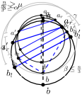
Figure 1: Left: the pair of parallel edges $b_{l}b_{l}^{\prime}$ and $a_{r}a_{r}^{\prime}$; center: case 1; right: case 2

Case 1. The edge $b_{l}b_{l}^{\prime}$ splits off $\mu\leq n/3$ vertices to the top; see Fig. 1 (center).

In this case, either $[b_{l}^{\prime},b]$ or $[b,b_{l}]$ has $[n/3,n/2]$ vertices. We claim that neither the line $bb_{l}$ nor the line $bb_{l}^{\prime}$ can be crossed more than $k$ times. Namely, each edge that crosses the line $bb_{l}$ also crosses the edge $b_{l}b_{l}^{\prime}$. Similarly, each edge that crosses the line $bb_{l}^{\prime}$ also crosses the edge $b_{l}b_{l}^{\prime}$. Thus, we have a separator of size at most $k+2$, regardless of whether we choose $bb_{l}$ or $bb_{l}^{\prime}$ to separate the graph. As we observed above, one of them is balanced.

Case 1^′. The edge $a_{r}a_{r}^{\prime}$ splits off at most $n/3$ vertices to the bottom.
This is symmetric to case 1.

Case 2. The edge $b_{l}b_{l}^{\prime}$ splits off at most $n/3$ vertices to the bottom, and the edge $a_{r}a_{r}^{\prime}$ splits off at most $n/3$ vertices to the top; see Fig. 1 (right).

We show that we can always find a pair of parallel edges such that one splits off at most $n/3$ vertices to the bottom and the other splits off at most $n/3$ vertices to the top, and no edge between them is parallel to either of them. We call such a pair close. If there is an edge $e$ between $b_{l}b_{l}^{\prime}$ and $a_{r}a_{r}^{\prime}$, we form a new pair by using $e$ and $a_{r}a_{r}^{\prime}$ if $e$ splits off at most $n/3$ vertices to the bottom or by using $e$ and $b_{l}b_{l}^{\prime}$ if $e$ splits off at most $n/3$ vertices to the top. By repeating this procedure, we always find a close pair. Hence, we can assume that $b_{l}b_{l}^{\prime}$ and $a_{r}a_{r}^{\prime}$ actually form a close pair. Let $\alpha=|(a_{r}^{\prime},a_{r})|$, $\beta=|(b_{l}^{\prime},b_{l})|$, $\gamma=|(a_{r},b_{l}^{\prime})|$, and $\delta=|(b_{l},a_{r}^{\prime})|$; see Fig. 1 (right).

Suppose that $a_{r}^{\prime}=b_{l}$ or $a_{r}=b_{l}^{\prime}$. We can now use both edges $b_{l}b_{l}^{\prime}$ and $a_{r}a_{r}^{\prime}$ (together with any edges crossing them) to obtain a separator of size at most $2k+3$. The separator is balanced since $\alpha+\beta\leq{2n}/{3}$ and $\gamma+\delta\leq{2n}/{3}$.

So, now $a_{r},a_{r}^{\prime},b_{l},b_{l}^{\prime}$ are all distinct. Note that $\gamma,\delta\leq n/2$ since each side of the line $ab$ has at most $n/2$ vertices. We separate the graph along the line $b_{l}a_{r}$. Namely, all the edges that cross this line must also cross $b_{l}b_{l}^{\prime}$ or $a_{r}^{\prime}a_{r}$. Therefore, we obtain a separator of size at most $2k+2$.

To see that the separator is balanced, we consider two cases. If $\delta\geq{n}/{3}$ (or $\gamma\geq{n}/{3}$), then $\alpha+\beta+\gamma\leq{2n}/{3}$ (or $\alpha+\beta+\delta\leq{2n}/{3}$). Otherwise $\delta<n/3$ and $\gamma<{n}/{3}$. In this case $\delta+\alpha\leq{2n}/{3}$ and $\gamma+\beta\leq{2n}/{3}$. In both cases the separator is balanced.

Theorem 2.7.

For fixed $k$, testing the outer $k$-planarity of an $n$-vertex graph takes $O(2^{\mathrm{polylog}(n)})$ time.

Figure 2: Shapes of separators, special separator $S$ in blue, regions in different colors (red, orange, and pink), components connected to blue vertices in green: (a) closest-parallels case; (b) single-edge case; (c) special case for single-edge separators.

Proof 2.8.

Our approach is to leverage the structure of the balanced separators as described in the proof of Theorem 2.5. Namely, we enumerate the sets which could correspond to such a separator, pick an appropriate outer $k$-planar drawing of these vertices and their edges, partition the components arising from this separator into regions, and recursively test the outer $k$-planarity of the regions.

To obtain quasi-polynomial runtime, we need to limit the number of components on which we branch. To do so, we group them into regions defined by special edges of the separators.

By the proof of Theorem 2.5, if our input graph has an outer $k$-planar drawing, there must be a separator which has one of the two shapes depicted in Fig. 2 (a) and (b). Here we are not only interested in the up to $2k+3$ vertices of the balanced separator, but in the set $S$ of up to $4k+3$ vertices that one obtains by taking both endpoints of the edges used to find the separator. Note: $S$ is also a balanced separator. We use a brute force approach to find such an $S$. Namely, we first enumerate vertex sets of size up to $4k+3$. We then consider two possibilities, i.e., whether this set can be drawn similar to one of the two shapes from Fig. 2. So, we now fix this set $S$. Note that since $S$ has $O(k)$ vertices, the subgraph $G_{S}$ induced by $S$ can have at most a function of $k$ different outer $k$-planar drawings. Thus, we further fix a particular drawing of $G_{S}$.

We now consider the two different shapes separately. In the first case, in $S$, we have three special vertices $v,w_{1}$ and $w_{2}$ and in the second case we will have two special vertices $v$ and $w$. These vertices will be called boundary vertices and all other vertices in $S$ will be called regional vertices. Note that, since we have a fixed drawing of $G_{S}$, the regional vertices are partitioned into regions by the specially chosen boundary vertices. Now, from the structure of the separator which is guaranteed by the proof of Theorem 2.5, no component of $G\setminus S$ can be adjacent to regional vertices which live in different regions with respect to the boundary vertices.

We first discuss the case of using $G_{S}$ as depicted in Fig. 2 (a). Here, we start by picking the three special vertices $v,w_{1}$ and $w_{2}$ from $S$ to take the role as shown in Fig. 2 (a). The following arguments regarding this shape of separator are symmetric with respect to the pair of opposing regions.

Notice that if there is a component connected to regional vertices of different regions, we can reject this configuration. From the proof of Theorem 2.5, we further observe that no component can be adjacent to all three boundary vertices. Namely, this would contradict the closeness of the parallel edges or it would contradict the members of the separator, i.e., it would imply an edge connecting distinct regions. We now consider the four possible different types of components $c_{1},c_{2},c_{3}$ and $c_{4}$ in Fig. 2(a) that can occur in a region neighboring $w_{1}$. Components of type $c_{1}$ are connected to (possibly many) regional vertices of the same region and may be connected to boundary vertices as well. In any valid drawing, they will end up in the same region as their regional vertices. Components of type $c_{2}$ are not connected to any regional vertices and only connected to one of the three boundary vertices. Since they are not connected to regional vertices, they can not interfere with other parts of the drawing, so we can arbitrarily assign them to an adjacent region of their boundary vertex. Components that are connected to two boundary vertices appear at first to have two possible placements, e.g., as $c_{3}$ or $c_{4}$ in Fig. 2 (a). However, $c_{4}$ is not a valid placement for this type of component since it would contradict the fact that this separator arose from two close parallel edges as argued in the proof of Theorem 2.5. From the above discussion, we see that from a fixed configuration (i.e., set $S$, drawing of $G_{S}$, and triple of boundary vertices), if the drawing of $G_{S}$ has the shape depicted in Fig. 2 (a), we can either reject the current configuration (based on having bad components), or we see that every component of $G\setminus S$ is either attached to exactly one boundary vertex or it has a well-defined placement into the regions defined by the boundary vertices. For those components which are attached to exactly one boundary vertex, we observe that it suffices to recursively produce a drawing of that component together with its boundary vertex and to place this drawing next to the boundary vertex. For the other components, we partition them into their regions and recurse on the regions. This covers all cases for this separator shape.

The other shape of our separator can be seen in Fig. 2 (b). Note that we now have two boundary vertices $v$ and $w$ and thus only have two regions. Again we see the two component types $c_{1}$ and $c_{2}$ and can handle them as above. We also have components connected to both $v$ and $w$ but no regional vertices. These components now truly have two different placement options $c_{3},c_{4}$. If we have an edge $v_{i}w_{i}$ (as in Fig. 2 (b)) of the separator that is not $vw$, we now observe that there cannot be more than $k$ such components. Namely, in any drawing, for each component, there will be an edge connecting this component to either $v$ or $w$ which crosses $v_{i}w_{i}$. Thus, we now enumerate all the different placements of these components as type $c_{3}$ or $c_{4}$ and recurse accordingly.

However, the separator may be exactly the pair $(v,w)$. Note that there are no components of type $c_{1}$ and the components of type $c_{2}$ can be handled as before. We will now argue that we can have at most a function of $k$ different components of type $c_{3}$ or $c_{4}$ in a valid drawing. Consider the components of type $c_{3}$ (the components of type $c_{4}$ can be counted similarly). In a valid drawing, each type $c_{3}$ component defines a sub-interval of the left region spanning from its highest to its lowest vertex such that these vertices are adjacent to one of $v$ or $w$. Two such intervals relate in one of three ways: They overlap, they are disjoint, or one is contained in the other. We group components with either overlapping or disjoint intervals into layers. We depict this situation in Fig. 2 (c) where, for simplicity, for every component we only draw its highest vertex and its lowest vertex and they are connected by one edge.

Let $a_{1}b_{1}$ be the bottommost component of type $c_{3}$ (i.e., $a_{1}$ is the clockwise-first vertex from $v$ in a component of type $c_{3}$). The first layer is defined as the component $a_{1}b_{1}$ together with every component whose interval either overlaps or is disjoint from the interval of $a_{1}b_{1}$. Now consider the green edge $b_{1}w$ (see Fig. 2 (c)), note we may have that this edge connects $a_{1}$ to $w$ instead. Now, for every component of this layer which is disjoint from the interval of $a_{1}b_{1}$, this edge is crossed by at least one edge connecting it to $v$. Furthermore, for every component of this layer which overlaps the interval of $a_{1}b_{1}$, there is an edge connecting $b_{1}$ to either $v$ or $w$ which is crossed by at least one edge within that component. So in total, there can only be $O(k)$ components in this first layer. New layers are defined by considering components whose intervals are contained in $a_{1}b_{1}$. To limit the total number of layers, let $a_{\ell}$ be the bottommost vertex of the first component of the deepest layer and consider the purple edge $va_{\ell}$. This edge is crossed by some edge of every layer above it and as any edge can only have $k$ crossings, there can only be $O(k)$ different levels in total. This leaves us with a total of at most $O(k^{2})$ components per region and again we can enumerate their placements and recurse accordingly.

The above algorithm provides the following recurrence regarding its runtime. Let $T(n)$ denote the runtime of our algorithm for an outer $k$-planar graph with $n$ vertices. Then,

$$T(n)\leq\begin{cases}n^{O(k)}\cdot f(4k+3)\cdot n^{3}\cdot n\cdot T({2n}/{3})&\text{ for }n>5k,\\ f(n)&\text{ otherwise,}\\ \end{cases}$$

where $f(s)$ denotes the number of different outer $k$-planar drawings of a graph with $s$ vertices. The factor $n^{O(k)}$ stands for finding all possible separators of size $4k+3$, $f(4k+3)$ is the number of different outer $k$-planar drawings of such a separator, $n^{3}$ is the time needed to partition the remaining vertices of the graph into regions, $n$ is the largest number of different regions, and $T({2n}/{3})$ is the runtime of the recursive call on a region.

Thus, the algorithm runs in quasi-polynomial time, i.e., $T\in 2^{\mathrm{polylog}(n)}$.

3 Outer $k$-Quasi-Planar Graphs

In this section we consider outer $k$-quasi-planar graphs. We first describe some classes of graphs which are outer quasi-planar (outer 3-quasi-planar) and some classes of graphs that are not outer quasi-planar. In particular, we show that there are planar graphs which are not outer quasi-planar what yields the fact that planar graphs and quasi-planar graphs are incomparable; see Theorem 3.5.

Note that all sub-Hamiltonian planar graphs are outer quasi-planar. We now quickly check which complete and bipartite complete graphs are outer quasi-planar.

Proposition 3.1.

The following graphs are outer quasi-planar: (a) $K_{p,q}$ for $p\leq 4$ and $q\leq 4$; (b) $K_{n}$ for $n\leq 5$; (c) the planar $3$-tree with at most three complete levels; (d) square grids of any size.

Proof 3.2.

Figure 3 shows that $K_{4,4}$ and $K_{5}$ are outer quasi-planar. This yields claims (a) and (b). We verified claim (c) by constructing a Boolean expression and using MiniSat to check its satisfiability; see Appendix A. Claim (d) follows from the fact that square grids are sub-Hamiltonian.

Figure 3: Outer quasi-planar drawings of the graphs $K_{5}$ and $K_{4,4}$

Below, we identify complete and complete bipartite graphs that are not outer-quasi planar. Furthermore, not all planar graphs are outer quasi-planar, e.g., Fig. 4(a) shows a planar 3-tree that is not outer quasi-planar (but removing any vertex renders it outer quasi-planar). This was verified using a SAT formulation; see Appendix A. The drawing of the graph in Fig. 4(b) was constructed by removing the blue vertex and drawing the remaining graph in an outer quasi-planar way.

Proposition 3.3.

The following graphs are not outer quasi-planar: (a) $K_{p,q}$, for $p\geq 3$ and $q\geq 5$; (b) $K_{n}$, for $n\geq 6$; (c) every planar 3-tree with at least four complete levels.

Proof 3.4.

This was verified using the SAT formulation in Appendix A for $K_{3,5}$, $K_{6}$, and the planar 3-tree with four complete levels.

Together, Propositions 3.1 and 3.3 immediately yield the following.

Theorem 3.5.

Planar graphs and outer quasi-planar graphs are incomparable under containment.

Remark 3.6.

For outer $k$-quasi-planar graphs with $k>3$, containment questions become more intricate. Every planar graph is outer 5-quasi-planar because planar graphs have page number 4 [48]. There are planar graphs that are not outer quasi-planar (the planar 3-trees with at least four complete levels). It is open whether every planar graph is outer 4-quasi-planar.

(a)

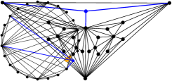
(b)

Figure 4: A planar 3-tree (with 23 vertices) that is not outer quasi-planar: (a) planar drawing; (b) deleting the blue vertex makes the drawing outer quasi-planar.

4 Testing for Full Convex Drawings via MSO₂

The class of full outer $k$-planar graphs was introduced by Hong and Nagamochi [32]. Recall that this class consists of the graphs that admit a $k$-planar convex drawing where no crossing lies on the boundary of the outer face. Hong and Nagamochi gave a linear-time recognition algorithm for full outer $2$-planar graphs. They state that a graph $G$ is (full) outer $2$-planar if and only if its biconnected components are (full) outer $2$-planar and that the outer boundary of a full outer $2$-planar embedding of a biconnected graph $G$ is a Hamiltonian cycle of $G$. We call the subclasses of outer $k$-planar and outer $k$-quasi-planar graphs that have a convex drawing where the circular order forms a Hamiltonian cycle closed outer $k$-planar and closed outer $k$-quasi-planar, respectively. We observe that the property stated by Hong and Nagamochi carries over to general outer $k$-planar and outer $k$-quasi-planar graphs.

A graph $G$ is full outer $k$-planar (outer $k$-quasi-planar) if and only if its biconnected components are closed outer $k$-planar (closed outer $k$-quasi-planar).

We show that we can encode closed outer $k$-planarity and closed outer $k$-quasi-planarity using Monadic Second-Order Logic (MSO₂). To do so, we initially give a brief introduction to MSO₂ and Courcelle’s theorem. Then we design MSO₂ formulas expressing crossing patterns of closed $k$-planar and closed $k$-quasi-planar drawings. Thus, using Observation 4, we can test full outer $k$-planarity (full outer $k$-quasi-planarity) of a graph $G$ by testing its biconnected components for closed outer $k$-planarity (closed outer $k$-quasi-planarity) using the MSO₂ formulas. This, together with Courcelle’s theorem (see Theorem 4.1) and the fact that outer $k$-planar graphs have bounded treewidth (see Proposition 8.5 of [47]) yields a linear-time algorithm for testing full outer $k$-planarity.

Monadic Second-Order Logic (MSO₂) – a subset of second-order logic – can be used to express certain graph properties. It is built from the following primitives.

• variables for vertices, edges, sets of vertices, and sets of edges;

• binary relations for: equality ($=$), membership in a set ($\in$), subset of a set ($\subseteq$), and edge–vertex incidence ($I$);

• standard propositional logic operators: $\lnot$, $\land$, $\lor$, $\rightarrow$, and $\leftrightarrow$.

• standard quantifiers ($\forall,\exists$) which can be applied to all types of variables.

For a graph $G$ and an MSO₂ formula $\phi$, we use $G\models\phi$ to indicate that $\phi$ can be satisfied by $G$ in the obvious way. Properties expressed in this logic allow us to use the powerful algorithmic result of Courcelle stated next.

Theorem 4.1 ([19, 20]).

For any integer $t\geq 0$ and any MSO₂ formula $\phi$ of length $\ell$, an algorithm can be constructed that takes a graph $G$ with $n$ vertices, $m$ edges, and treewidth at most $t$, and decides whether $G\models\phi$ in time $O(f(t,\ell)\cdot(n+m))$, where the function $f$ is computable.

The challenge in expressing outer $k$-planarity or outer $k$-quasi-planarity in MSO₂ is that MSO₂ does not allow quantification over sets of pairs of vertices which involve non-edges. Namely, it is unclear how to express a set of pairs that forms the circular order of vertices on the boundary of our convex drawing. However, if this circular order forms a Hamiltonian cycle in our graph, i.e., the given graph is closed, then we can indeed express this in MSO₂. With the edge set of a Hamiltonian cycle of our graph in hand, we can then ask that this cycle was chosen in such a way that the other edges satisfy either $k$-planarity or $k$-quasi-planarity.

The MSO₂ formulas presented below assume that a graph $G$ is given and uses the edges, vertices, and incidences of $G$. In the following, $V$ is the vertex set of $G$, $u,v\in V$, and $U\subseteq V$. Further, $E$ is the edge set of $G$, $e,f\in E$, and $F\subseteq E$. (We also use sub- and superscripted variants of these variables.) In addition to the quantifiers above, we use $\exists^{=x}$ as shorthand to express the existence of exactly $x$ (but no $x+1$) pairwise different elements satisfying a property.

The first formula expresses the connectivity of a subgraph induced by a given edge set $F$.

$\textsc{Connected-Edges}(F)\equiv(\forall F^{\prime})\big{(}[F^{\prime}\neq\emptyset\wedge F^{\prime}\subsetneq F]\rightarrow$
$\textsc{Connected-Edges}(F)\equiv(\forall F^{\prime})\big{(}$$(\exists e,f,v)[e\in F^{\prime}\wedge f\in F\setminus F^{\prime}\wedge v\in V\wedge I(e,v)\wedge I(f,v)]\big{)}$

It states that, for every nonempty proper subset $F^{\prime}$ of the given edge set $F$, we can find an edge $e$ in $F^{\prime}$, an edge $f$ in $F\setminus F^{\prime}$, and a vertex that is incident to both.

We use the predicate Connected-Edges$(F)$ and the following predicates to express the Hamiltonicity of $G$. The predicate Cycle-Set$(F)$ expresses that $F$ forms a set of cycles, Cycle$(F)$ expresses that $F$ consists of a single cycle, and Span$(F)$ forces $F$ to span $G$.

$$\textsc{Cycle-Set}(F) \equiv(\forall e)\Big{[}e\in F\rightarrow(\exists^{=2}f)\big{[}f\in F\wedge e\neq f\wedge(\exists v)[I(e,v)\wedge I(f,v)]\big{]}\Big{]}$$

$$\textsc{Cycle}(F) \equiv\textsc{Cycle-Set}(F)\wedge\textsc{Connected-Edges}(F)$$

$$\textsc{Span}(F) \equiv(\forall v)(\exists e)[e\in F\wedge I(e,v)]$$

$$\textsc{Hamiltonian}(F) \equiv[\textsc{Cycle}(F)\wedge\textsc{Span}(F)]$$

The following predicate Vertex-Partition expresses the existence of a partition of the vertices of $G$ into $k$ disjoint subsets.

$$\textsc{Vertex-Partition}(U_{1},\dots,U_{k})\equiv(\forall v)\left[\left(\bigvee_{i=1}^{k}v\in U_{k}\right)\wedge\left(\bigwedge_{i\neq j}\neg(v\in U_{i}\wedge v\in U_{j})\right)\right]$$

For a closed outer $k$-planar or closed outer $k$-quasi-planar graph $G$, we want to express that two edges $e$ and $e_{i}$ cross. To this end, we assume that there is a Hamiltonian cycle $E^{*}$ of $G$ that defines the outer face. We partition the vertices of $G$ into three subsets $C$, $A$, and $B$, as follows: $C$ is the set containing the endpoints of $e$, whereas $A$ and $B$ are connected subgraphs on the remaining vertices that use only edges of $E^{*}$. In this way, we partition the vertices of $G$ into two sets, one left and the other one right of $e$. For such a partition, $e_{i}$ must cross $e$ whenever $e_{i}$ has one endpoint in $A$ and one in $B$.

Cro $$\textsc{ssing}(E^{*},e,e_{i})\equiv(\forall A,B,C)\big{[}\big{(}\textsc{Vertex-Partition}(A,B,C)$$

$$\wedge(I(e,x)\leftrightarrow x\in C)\wedge\textsc{Connected}(A,E^{*})\wedge\textsc{Connected}(B,E^{*})\big{)}$$

$$\rightarrow(\exists a\in A)(\exists b\in B)[I(e_{i},a)\wedge I(e_{i},b)]\big{]}$$

Now we can describe the crossing patterns for closed outer $k$-planarity and closed outer $k$-quasi-planarity as follows:

$$\textsc{Closed Outer $k$-Planar}_{G}\equiv(\exists E^{*})\Big{[}\textsc{Hamiltonian}(E^{*})\wedge$$

$$(\forall e)\Big{[}(\forall e_{1},\dots,e_{k+1})\Big{[}\Big{(}\bigwedge_{i=1}^{k+1}e_{i}\neq e\wedge\bigwedge_{i\neq j}e_{i}\neq e_{j}\Big{)}\rightarrow\bigvee_{i=1}^{k+1}\neg\textsc{Crossing}(E^{*},e,e_{i})\Big{]}\Big{]}\Big{]}$$

Here we insist that $G$ is Hamiltonian and that, for every edge $e$ and any set of $k+1$ distinct other edges, at least one among them does not cross $e$.

$$\textsc{Closed Outer $k$-Quasi-Planar}_{G}\equiv(\exists E^{*})\Big{[}\textsc{Hamiltonian}(E^{*})\wedge$$

$$(\forall e_{1},\dots,e_{k})\Big{[}\Big{(}\bigwedge_{i\neq j}e_{i}\neq e_{j}\Big{)}\rightarrow\bigvee_{i\neq j}\neg\textsc{Crossing}(E^{*},e_{i},e_{j})\Big{]}\Big{]}$$

Again, we insist that $G$ is Hamiltonian and further that, for any set of $k$ distinct edges, there is at least one pair among them that does not cross.

The formulas above give us the following.

Theorem 4.2.

Closed outer $k$-planarity and closed outer $k$-quasi-planarity can be expressed in MSO₂ with a formula whose size depends only on $k$.

Theorem 4.3.

We can test whether a graph $G$ is full outer $k$-planar in linear time.

Proof 4.4.

Recall that in a full outer $k$-planar drawing there is no crossing on the outer boundary of the drawing and each biconnected component of the graph with such a drawing is a closed outer $k$-planar graph (Observation 4). Thus, in order to test full outer $k$-planarity for a given graph $G$ it suffices to test whether each of its biconnected components admits a closed outer $k$-planar drawing. We can break up $G$ into biconnected components in linear time by obtaining the set of cutvertices. Checking each biconnected component for closed outer $k$-planarity can be done via the above MSO₂ formula in time linear in the size of the component. The formula also guarantees that the Hamiltonian cycle (if present) is placed on the outer boundary of the drawing of each component. We put the individual drawings of the components together by reidentifying the cutvertices and without introducing any crossings. This can also be done in linear time. Thus, the total runtime is linear in the size of the input graph $G$.

Alternatively, we could encode the recognition of full outer $k$-planar graphs directly using an MSO₂ formula. This, however, will be more time consuming than the above approach.

5 Discussions and Open Problems

Every planar graph is outer $5$-quasi-planar because planar graphs have page number 4 [48]. (Planar graphs that require four pages have been discovered recently [49, 12]). There are also planar graphs that are not outer quasi-planar. The following question is still open.

Question 5.1.

Is every planar graph outer 4-quasi-planar?

We now discuss the relation between our crossing-restricted convex drawings and the class of intersection graphs of chords of a circle, i.e., circle graphs. Such representations are called chord diagrams. Here, a convex drawing $D$ of a graph $G$ can be seen as a chord diagram and as such provides a corresponding graph $H$ where each adjacency between two vertices corresponds to a crossing between the edges of our drawing. Independent sets in $H$ correspond to collections of pairwise non-crossing edges in $D$, i.e., outerplanar sub-drawings of $D$. Thus, $k$-coloring $H$ corresponds to partitioning $D$ into edge sets $E_{1},\ldots,E_{k}$ such that each sub-drawing of $D$ formed by the edges of $E_{i}$ is outerplanar. That is, the partition $E_{1},\ldots,E_{k}$ forms a book embedding of $G$ with $k$ pages. So, $k$-coloring the chord diagram provides a $k$-page book embedding of $G$. Interestingly, it is NP-complete to test whether a chord diagram can be 4-colored [28], but testing whether it can be 3-colored is still open [46]. On the other hand, circle graphs are $\chi$-bounded [37], i.e., the chromatic number $\chi(G)$ of a circle graph $G$ is bounded by a function of the clique number $\omega(G)$ of $G$, that is, the number of vertices in the maximum clique of $G$. Until recently the best known bound was $7\omega^{2}$ due to Davis et al. [23], but then Davis announced [22] an improved bound of $O(\omega\log{\omega})$, which is asymptotically tight. In particular, this means that every outer $k$-quasi planar drawing can be partitioned into $O(k\log{k})$ pages (since we cannot have $k$ mutually crossing edges, i.e., there is no $k$-clique in the corresponding intersection graph). For quasi-planar graphs ($k=3$) there is a tighter bound. Ageev [4] showed that any triangle-free circle graph has chromatic number at most 5. Because for a fixed drawing of an outer quasi-planar graph its corresponding circle graph is triangle-free, it has chromatic number at most 5, and thus, we can embed the outer quasi-planar graph in a book with five pages. An immediate open question is to improve this bound on the page number.

Ageev [4] constructed a triangle-free circle graph $G_{\mathrm{ageev}}$ with $\chi(G_{\mathrm{ageev}})=5$. The drawing of the outer quasi-planar graph $G$ corresponding to the circle graph $G_{\mathrm{ageev}}$ cannot be embedded on four pages because the circle graph has chromatic number 5. It turns out, however, that there exists a linear order of the vertices under which $G$ can be embedded on four pages, even if we add edges to make it maximal, but there does not exist such an order with the additional property that the drawing is outer quasi-planar. We have verified this experimentally by constructing a logical formula that tests outer quasi-planarity and 4-page embeddability at the same time; see Appendix A.

Question 5.2.

Does every outer quasi-planar graph have page number at most 4?

We also point to the gap between the lower bound (see Observation 2.1) and the upper bound (see Theorem 2.1) for the degeneracy of outer $k$-planar graphs.

Question 5.3.

Can we improve the lower bound of ${\lfloor\sqrt{4k+1}\rfloor+1}$ or the upper bound of $\lfloor 3.5\sqrt{k}\rfloor$ on the degeneracy of outer $k$-planar graphs?

There are several interesting questions from an algorithmic point of view.

Question 5.4.

Can we improve the quasi-polynomial algorithm in Theorem 2.7 to a polynomial one?

The linear runtime algorithm for testing full outer $k$-planarity in Theorem 4.3 relies on the Courcelle’s machinery for solving MSO₂ logic formulas and, therefore, has notoriously bad runtime dependence of $2^{O(k^{2})}$ on the parameter $k$. Therefore, in light of a similar result for one-page crossing minimization [35], it is natural to ask whether this can be improved:

Question 5.5.

Is there an explicit dynamic programming algorithm to decide whether a graph $G$ is full outer $k$-planar with a better runtime dependence on the parameter $k$?

Question 5.6.

Going beyond Questions 5.4 and 5.5, can we obtain an XP or a fixed-parameter tractable algorithm for testing general outer $k$-planarity?

Last but not least:

Question 5.7.

What is the complexity of outer $k$-quasi-planarity testing?

In general $k$-quasi-planarity testing has notoriously eluded the efforts to establish its computational complexity even for $k=3$ (or simply, quasi-planarity testing, with respect to our definition). Recently, Angelini et al. [8] showed that testing 2-level quasi-planarity (i.e., quasi-planarity for a bipartite graph in a 2-layer layout, where the vertices of each partition are on one of two parallel lines and the edges are drawn between the lines) is NP-complete, making first progress in this direction. Can this be adapted to show NP-completeness for testing outer $k$-quasi-planarity for any $k\geq 3$?

Appendix A SAT Formulations

In the following two sections we describe SAT formulations that can be used to test whether a given graph is outer quasi-planar (Section A.1) and to compute its page number (Section A.2). We present the formulas in first-order logic. After transformation to Boolean logic, the resulting formulas can be solved using, e.g., MiniSat (see http://minisat.se/).

A.1 Outer Quasi-Planarity Checker

In this section, we describe a logical formula for testing whether a given graph $G$ is outer quasi-planar. A quasi outer-planar embedding corresponds to a circular order of the vertices. If we cut a circular order at some vertex to turn the circular into a linear order, the edge crossing pattern remains the same. Therefore, we look for a linear order. For any pair of vertices $u\neq v\in V(G)$, we introduce a Boolean variable $x_{u,v}$ that expresses that vertex $u$ is before $v$ in the linear order. In addition, for any pair of edges $e\neq e^{\prime}\in E(G)$, we introduce a Boolean variable $y_{e,e^{\prime}}$ that expresses that edge $e$ crosses edge $e^{\prime}$. Now we list the clauses of our SAT formula.

$$x_{u,v}\wedge x_{v,w}\Rightarrow x_{u,w} \text{for each }u\neq v\neq w\neq u\in V(G);$$ (5)

$$x_{u,v}\Leftrightarrow\neg x_{v,u} \text{for each }u\neq v\in V(G);$$ (6)

$$x_{u,u^{\prime}}\wedge x_{u^{\prime},v}\wedge x_{v,v^{\prime}}\Rightarrow y_{e,e^{\prime}} \text{for each }e=(u,v)\;\neq\;e^{\prime}=(u^{\prime},v^{\prime})\in E(G);$$ (7)

$$\neg(y_{e_{1},e_{2}}\wedge y_{e_{1},e_{3}}\wedge y_{e_{2},e_{3}}) \text{for each }e_{1},e_{2},e_{3}\in E(G)\text{ with different endpoints.}$$ (8)

The first two sets of clauses describe the linear order. Clause (5) ensures transitivity, and clause (6) anti-symmetry. Clause (7) realizes the intended meaning of variable $y_{e,e^{\prime}}$. Finally, clause (8) ensures that no three edges pairwise cross.

A.2 Page Number Checker

In this section we provide a SAT formula that, given a graph $G$ and an integer $k>0$, has a satisfying truth assignment if and only if $G$ has page number at most $k$. A similar SAT solver has been implemented by Pupyrev [42] (see http://be.cs.arizona.edu/). For completeness, we list the constraints that we used in order to compute the page number of $G_{\mathrm{ageev}}$ (see Question 5.2). We find a linear order of the vertices that corresponds to a $k$-page embedding. For every pair of vertices $u\neq v\in V(G)$, we introduce a Boolean variable $x_{u,v}$ (as in Section A.1) that expresses that $u$ is before $v$ in the linear order. For every edge $e\in E(G)$ and page $i\in\mathcal{P}=\{1,\dots k\}$, we introduce a Boolean variable $p_{i,e}$ that expresses that edge $e$ is on page $i$. Now we list the clauses of our SAT formula.

$$(x_{u,v}\wedge x_{v,w})\Rightarrow x_{u,w} \text{ for each }u\neq v\neq w\neq u\in V(G);$$ (9)

$$x_{u,v}\Leftrightarrow\neg x_{v,u} \text{ for each }u\neq v\in V(G);$$ (10)

$$\bigvee_{i\in\mathcal{P}}p_{i,e} \text{ for each }e\in E(G);$$ (11)

$$(p_{i,e}\wedge p_{i,e^{\prime}})\Rightarrow\neg(x_{u,u^{\prime}}\wedge x_{u^{\prime},v}\wedge x_{v,v^{\prime}}) \text{ for each }i\in\mathcal{P},u\neq u^{\prime},v\neq v^{\prime}\in V(G),$$ (12)

$$\quad e=(u,v),e^{\prime}=(u^{\prime},v^{\prime})\in E(G)$$ (13)

The first two sets of clauses are the same as Clauses (5)–(6) since they describe the linear order. Clauses (11) guarantee that every edge is on some page. Clauses (12) ensure that two edges that have different endpoints and lie on the same page do not cross. (If two edges share an endpoint, they cannot cross.)

References

- [1] Eyal Ackerman. On the maximum number of edges in topological graphs with no four pairwise crossing edges. Discrete Comput. Geom., 41(3):365–375, 2009. doi:10.1007/s00454-009-9143-9.
- [2] Eyal Ackerman. On topological graphs with at most four crossings per edge. Comput. Geom., 85:101574, 2019. doi:10.1016/j.comgeo.2019.101574.
- [3] Eyal Ackerman and Gábor Tardos. On the maximum number of edges in quasi-planar graphs. J. Combin. Theory Ser. A, 114(3):563–571, 2007. doi:10.1016/j.jcta.2006.08.002.
- [4] Alexander A. Ageev. A triangle-free circle graph with chromatic number 5. Discrete Math., 152(1):295–298, 1996. doi:10.1016/0012-365X(95)00349-2.
- [5] Oswin Aichholzer, Johannes Obenaus, Joachim Orthaber, Rosna Paul, Patrick Schnider, Raphael Steiner, Tim Taubner, and Birgit Vogtenhuber. Edge partitions of complete geometric graphs. In Xavier Goaoc and Michael Kerber, editors, Proc. 38th Int. Symp. Comput. Geom. (SoCG 2022), volume 224 of LIPIcs, pages 6:1–6:16. Schloss Dagstuhl – Leibniz-Zentrum für Informatik, 2022. doi:10.4230/LIPIcs.SoCG.2022.6.
- [6] Patrizio Angelini, Michael A. Bekos, Franz J. Brandenburg, Giordano Da Lozzo, Giuseppe Di Battista, Walter Didimo, Michael Hoffmann, Giuseppe Liotta, Fabrizio Montecchiani, Ignaz Rutter, and Csaba D. Tóth. Simple -planar graphs are simple -quasiplanar. J. Combin. Theory Ser. B, 142:1–35, 2020. doi:10.1016/j.jctb.2019.08.006.
- [7] Patrizio Angelini, Giordano Da Lozzo, Henry Förster, and Thomas Schneck. 2-layer -planar graphs. In David Auber and Pavel Valtr, editors, GD 2020, volume 12590 of LNCS, pages 403–419. Springer, 2019. doi:10.1007/978-3-030-68766-3_32.
- [8] Patrizio Angelini, Giordano Da Lozzo, Giuseppe Di Battista, Fabrizio Frati, and Maurizio Patrignani. 2-level quasi-planarity or how caterpillars climb (SPQR-)trees. In Dániel Marx, editor, Proc. ACM-SIAM Symp. Discrete Algorithms, pages 2779–2798, 2021. doi:10.1137/1.9781611976465.165.
- [9] Christopher Auer, Christian Bachmaier, Franz J. Brandenburg, Andreas Gleißner, Kathrin Hanauer, Daniel Neuwirth, and Josef Reislhuber. Outer -planar graphs. Algorithmica, 74(4):1293–1320, 2016. doi:10.1007/s00453-015-0002-1.
- [10] Jasine Babu, Areej Khoury, and Ilan Newman. Every property of outerplanar graphs is testable. In Klaus Jansen, Claire Mathieu, José D. P. Rolim, and Chris Umans, editors, APPROX/RANDOM 2016, volume 60 of LIPIcs, pages 21:1–21:19. Schloss Dagstuhl – Leibniz-Zentrum für Informatik, 2016. doi:10.4230/LIPIcs.APPROX-RANDOM.2016.21.
- [11] Michael J. Bannister and David Eppstein. Crossing minimization for 1-page and 2-page drawings of graphs with bounded treewidth. Journal of Graph Algorithms and Applications, 22(4):577–606, 2018. doi:10.7155/jgaa.00479.
- [12] Michael A. Bekos, Michael Kaufmann, Fabian Klute, Sergey Pupyrev, Chrysanthi N. Raftopoulou, and Torsten Ueckerdt. Four pages are indeed necessary for planar graphs. J. Comput. Geom., 11(1):332–353, 2020. doi:10.20382/jocg.v11i1a12.
- [13] Carla Binucci, Emilio Di Giacomo, Md. Iqbal Hossain, and Giuseppe Liotta. 1-page and 2-page drawings with bounded number of crossings per edge. Eur. J. Comb., 68(Supplement C):24–37, 2018. doi:10.1016/j.ejc.2017.07.009.
- [14] Oleg V. Borodin. Solution of the Ringel problem on vertex-face coloring of planar graphs and coloring of -planar graphs. Metody Diskret. Analiz., 41:12–26, 108, 1984.
- [15] Franz J. Brandenburg. On fan-crossing and fan-crossing free graphs. Inform. Process. Lett., 138:67–71, 2018. doi:10.1016/j.ipl.2018.06.006.
- [16] Harry Buhrman and Steven Homer. Superpolynomial circuits, almost sparse oracles and the exponential hierarchy. In R. K. Shyamasundar, editor, Proc. 12th Conf. Foundat. Software Techn. Theoret. Comput. Sci. (FSTTCS), volume 652 of LNCS, pages 116–127. Springer, 1992. doi:10.1007/3-540-56287-7_99.
- [17] Vasilis Capoyleas and János Pach. A Turán-type theorem on chords of a convex polygon. J. Combin. Theory Ser. B, 56(1):9–15, 1992. doi:10.1016/0095-8956(92)90003-G.
- [18] Steven Chaplick, Thomas C. van Dijk, Myroslav Kryven, Ji-won Park, Alexander Ravsky, and Alexander Wolff. Bundled crossings revisited. J. Graph Algorithms Appl., 24(4):621–655, 2020. doi:10.7155/jgaa.00535.
- [19] Bruno Courcelle. The monadic second-order logic of graphs. I. Recognizable sets of finite graphs. Inform. Comput., 85(1):12–75, 1990. doi:10.1016/0890-5401(90)90043-H.
- [20] Bruno Courcelle and J. Engelfriet. Graph Structure and Monadic Second-Order Logic: A Language-Theoretic Approach. Cambridge University Press, 2012.
- [21] Marek Cygan, Fedor V. Fomin, Łukasz Kowalik, Daniel Lokshtanov, Dániel Marx, Marcin Pilipczuk, Michał Pilipczuk, and Saket Saurabh. Lower bounds based on the Exponential-Time Hypothesis. In Parameterized Algorithms, pages 467–521. Springer, 2015. doi:10.1007/978-3-319-21275-3_14.
- [22] James Davies. Improved bounds for colouring circle graphs. ArXiv, 2022. URL: https://arxiv.org/abs/2107.03585.
- [23] James Davies and Rose McCarty. Circle graphs are quadratically -bounded. Bull. London Math. Soc., 53(3):673–679, 2021. doi:10.1112/blms.12447.
- [24] Andreas W. M. Dress, Jack H. Koolen, and Vincent Moulton. On line arrangements in the hyperbolic plane. Eur. J. Comb., 23(5):549–557, 2002. doi:10.1006/eujc.2002.0582.
- [25] Vida Dujmović, David Eppstein, and David R. Wood. Structure of graphs with locally restricted crossings. SIAM J. Discrete Math., 31(2):805–824, 2017. doi:10.1137/16M1062879.
- [26] Zdenek Dvořák and Sergey Norin. Treewidth of graphs with balanced separations. J. Comb. Theory Ser. B, 137:137–144, 2019. doi:10.1016/j.jctb.2018.12.007.
- [27] Jacob Fox, János Pach, and Andrew Suk. Quasiplanar graphs, string graphs, and the Erdös-Gallai problem. In Patrizio Angelini and Reinhard von Hanxleden, editors, GD 2022, volume 13764 of LNCS. Springer, 2022. doi:10.1007/978-3-031-22203-0_16.
- [28] M. R. Garey, D. S. Johnson, Gary L. Miller, and C. H. Papadimitriou. The complexity of coloring circular arcs and chords. SIAM J. Alg. Disc. Meth., 1(2):216–227, 1980.
- [29] Jesse Geneson, Tanya Khovanova, and Jonathan Tidor. Convex geometric ()-quasiplanar representations of semi-bar -visibility graphs. Discrete Math., 331:83–88, 2014. doi:10.1016/j.disc.2014.05.001.
- [30] Danny Holten. Hierarchical edge bundles: Visualization of adjacency relations in hierarchical data. IEEE Trans. Vis. Comput. Graphics, 12(5):741–748, 2006. doi:10.1109/TVCG.2006.147.
- [31] Seok-Hee Hong, Peter Eades, Naoki Katoh, Giuseppe Liotta, Pascal Schweitzer, and Yusuke Suzuki. A linear-time algorithm for testing outer-1-planarity. Algorithmica, 72(4):1033–1054, 2015. doi:10.1007/s00453-014-9890-8.
- [32] Seok-Hee Hong and Hiroshi Nagamochi. A linear-time algorithm for testing full outer-2-planarity. Discret. Appl. Math., 255:234–257, 2019. doi:10.1016/j.dam.2018.08.018.
- [33] Russell Impagliazzo and Ramamohan Paturi. On the complexity of -SAT. J. Comput. Syst. Sci., 62(2):367–375, 2001. doi:10.1006/jcss.2000.1727.
- [34] Ken-ichi Kawarabayashi and Buce Reed. Computing crossing number in linear time. In Proc. 39th Ann. ACM Symp. Theory Comput., pages 382–390, 2007. doi:10.1145/1250790.1250848.
- [35] Yasuaki Kobayashi, Hiromu Ohtsuka, and Hisao Tamaki. An improved fixed-parameter algorithm for one-page crossing minimization. In Daniel Lokshtanov and Naomi Nishimura, editors, Proc. 12th International Symposium on Parameterized and Exact Computation (IPEC 2017), volume 89 of LIPIcs, pages 25:1–25:12. Schloss Dagstuhl – Leibniz-Zentrum für Informatik, 2018. doi:10.4230/LIPIcs.IPEC.2017.25.
- [36] Stephen G. Kobourov, Giuseppe Liotta, and Fabrizio Montecchiani. An annotated bibliography on 1-planarity. Comput. Sci. Rev., 25:49–67, 2017. doi:10.1016/j.cosrev.2017.06.002.
- [37] Alexandr Kostochka and Jan Kratochvíl. Covering and coloring polygon-circle graphs. Discrete Math., 163(1):299–305, 1997. doi:10.1016/S0012-365X(96)00344-5.
- [38] Don R. Lick and Arthur T. White. -degenerate graphs. Canadian J. Math., 22:1082–1096, 1970. doi:10.4153/CJM-1970-125-1.
- [39] Sumio Masuda, Toshinobu Kashiwabara, Kazuo Nakajima, and Toshio Fujisawa. On the NP-completeness of a computer network layout problem. In Proc. IEEE Int. Symp. Circuits and Systems, pages 292–295, 1987.
- [40] Tomoki Nakamigawa. A generalization of diagonal flips in a convex polygon. Theor. Comput. Sci., 235(2):271–282, 2000. doi:10.1016/S0304-3975(99)00199-1.
- [41] J. Pach, F. Shahrokhi, and M. Szegedy. Applications of the crossing number. Algorithmica, 16(1):111–117, 1996. doi:10.1007/BF02086610.
- [42] Sergey Pupyrev. Mixed linear layouts of planar graphs. In Fabrizio Frati and Kwan-Liu Ma, editors, GD 2017, volume 10692 of LNCS, pages 197–209. Springer, 2017. doi:10.1007/978-3-319-73915-1\_17.
- [43] Gerhard Ringel. Ein Sechsfarbenproblem auf der Kugel. Abhandlungen aus dem Mathematischen Seminar der Universität Hamburg, 29(1):107–117, 1965. doi:10.1007/BF02996313.
- [44] Neil Robertson and Paul D. Seymour. Graph minors. III. Planar tree-width. J. Combin. Theory Ser. B, 36(1):49–64, 1984. doi:10.1016/0095-8956(84)90013-3.
- [45] Marcus Schaefer. The graph crossing number and its variants: A survey. Electronic J. Combin., DS21:100 pages, 2022. doi:10.37236/2713.
- [46] Wikipedia. Circle graph — Wikipedia, The Free Encyclopedia, 2016. [Online; accessed 10-June-2017]. URL: https://en.wikipedia.org/w/index.php?title=Circle_graph&oldid=705761079.
- [47] David R. Wood and Jan Arne Telle. Planar decompositions and the crossing number of graphs with an excluded minor. New York J. Math., 13:117–146, 2007.
- [48] Mihalis Yannakakis. Embedding planar graphs in four pages. J. Comput. Syst. Sci., 38(1):36–67, 1989. doi:10.1016/0022-0000(89)90032-9.
- [49] Mihalis Yannakakis. Planar graphs that need four pages. J. Combin. Theory Ser. B, 145:241–263, 2020. doi:10.1016/j.jctb.2020.05.008.