Better together? Statistical learning in models made of modules

Abstract

In modern applications, statisticians are faced with integrating heterogeneous data modalities relevant for an inference, prediction, or decision problem. In such circumstances, it is convenient to use a graphical model to represent the statistical dependencies, via a set of connected ‘modules’, each relating to a specific data modality, and drawing on specific domain expertise in their development. In principle, given data, the conventional statistical update then allows for coherent uncertainty quantification and information propagation through and across the modules. However, misspecification of any module can contaminate the estimate and update of others, often in unpredictable ways. In various settings, particularly when certain modules are trusted more than others, practitioners have preferred to avoid learning with the full model in favor of approaches that restrict the information propagation between modules, for example by restricting propagation to only particular directions along the edges of the graph. In this article, we investigate why these modular approaches might be preferable to the full model in misspecified settings. We propose principled criteria to choose between modular and full-model approaches. The question arises in many applied settings, including large stochastic dynamical systems, meta-analysis, epidemiological models, air pollution models, pharmacokinetics-pharmacodynamics, and causal inference with propensity scores.

1 Introduction

1.1 The setting

Consider the situation where a statistical model has been assembled from different components, which we call modules. Each of these may have been developed by a separate community, or built using specific domain knowledge of a particular data modality. Such joint models, sometimes termed hierarchical (Robert, 2007), super (Shen et al., 2016), or coupled (Béal et al., 2010) models, are becoming widespread as measurement technologies and data storage become cheap, and as efforts to quantify uncertainty intensify. For example, in a model relating air pollution to human health, the joint model might be made of an air pollution component, guided by climate science and data from monitoring stations, and a component for human health, based on medical science and electronic health records (see e.g. Blangiardo et al., 2011).

In principle, conventional statistical updating tackles all modules jointly with the advantage that all uncertainties can be treated simultaneously and coherently. This is achieved by the posterior distribution in ideal settings (Bernardo and Smith, 2009; Gelman et al., 2014). However, in a joint model where information flows both ways between any pair of modules, misspecification of either leads to misspecification of the full model (Liu et al., 2009), potentially leading to misleading quantification of uncertainties (Grünwald, 2012; Kleijn and van der Vaart, 2012; Müller, 2013). This motivates approaches that depart from learning with the full model. There may also be other motivations to eschew the full model, such as computational constraints and data confidentiality.

To understand the problem and the statistical issues that arise in its simplest form, consider a graphical model made of just two modules as shown in Figure 1. In the first module we observe data modality $Y_{1}$ with a corresponding likelihood $p_{1}(Y_{1}|\theta_{1})$ parameterized by $\theta_{1}$. We will utilize a Bayesian formulation and a prior distribution $p_{1}(\theta_{1})$. In the absence of other information the inference on $\theta_{1}$ obtains the posterior distribution $\pi_{1}(\theta_{1}|Y_{1})\propto p_{1}(Y_{1}|\theta_{1})p_{1}(\theta_{1})$. Note that, in general, $\theta_{1}$ is simply an unknown of interest, for example a realization of a future observable, such that $\pi_{1}(\theta_{1}|Y_{1})$ represents a predictive distribution. We are interested in the situation where $\theta_{1}$ is then used in a second module, introducing extra parameters $\theta_{2}$ and data $Y_{2}$. To make the second module operational, some knowledge on $\theta_{1}$ is required, so that its likelihood and prior distribution may depend on $\theta_{1}$. The likelihood of this second module is $p_{2}\left(Y_{2}|\theta_{1},\theta_{2}\right)$, and its prior distribution $p_{2}(\theta_{2}|\theta_{1})$. When all of the components are well specified then the joint model provides optimal learning about all of the unknowns (Zellner, 1988). However, for a number of reasons—model misspecification, numerous missing values in certain modalities, contamination of errors, a priori trust in the specification of some modules more than in others, computational constraints and data privacy—one might want to depart from this full model update.

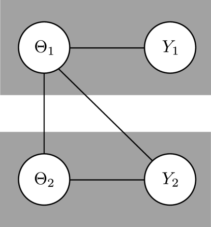
Figure 1: Variables involved in a model made of two modules. The first module has parameter $\theta_{1}$ and data $Y_{1}$, while the second is defined conditionally upon $\theta_{1}$, with parameter $\theta_{2}$ and data $Y_{2}$.

Departing from the full model then raises some crucial questions such as: can we cut the undesired feedback of some components on others without hampering uncertainty propagation? Can we design principled methods to decide whether to use the full model or modular approaches? Can we formalise the problem within a valid Bayesian framework? It is the aim of this article to facilitate answers to such questions and propose a principled way to proceed through the use of decision theoretic arguments. Following others (e.g. Liu et al., 2009), we refer to the general area of inference in models made of modules as “modularization”.

1.2 Background literature

Notions of modularization crop up in many applied settings, reviewed below, but the systematic statistical evaluation of the techniques has received relatively little attention in the methodology literature. Some general issues are described in Liu et al. (2009), with applications to computer model calibration. Computational challenges associated with certain modular approaches are discussed in Plummer (2014). Both of these articles present reproducible examples which we investigate in Section 4. In fact the concept of cutting feedback is already implemented in conventional Bayesian software such as WinBUGS which includes a ‘cut function’ for multiple imputation and plug-in or two-step approaches (Liu et al., 2009; Plummer, 2014). Specific examples of modularization appear in diverse applications, such as air pollution (Blangiardo et al., 2011), epidemiological models (Maucort-Boulch et al., 2008; Finucane et al., 2013; Li et al., 2017), pharmacokinetics-pharmacodynamics (Bennett and Wakefield, 2001; Lunn et al., 2009), meta-analysis (Lunn et al., 2013; Kaizar, 2015) and propensity scores (McCandless et al., 2010; Zigler et al., 2013; Zigler and Dominici, 2014).

The example of pharmacokinetics-pharmacodynamics (PKPD) is representative of the strong connection between modularization and misspecification. Pharmacokinetics (PK) is the study of the body’s effect on a drug, while pharmacodynamics (PD) is the study of a drug’s effect on the body. It is generally believed that the PK part is more precise, or at least better understood scientifically, than the PD part. This motivates, e.g. in Bennett and Wakefield (2001), a first module fit separately on the PK data, and a second module that uses the first inference in an errors-in-variables model for the PD part. In WinBUGS, the “cut” function is intended for such situations (Plummer, 2014). For instance, Lunn et al. (2009) consider “cutting” the feedback of information from variables in the PD module to variables in the PK module: “the four models considered [corresponding to various cuts] can be thought of as representing varying degrees of confidence in the PK model relative to the PD model” (p. 32). Thus, in PKPD studies, modular approaches are motivated by the suspected misspecification of the PD module.

Modular approaches are routinely used in econometrics (e.g. Pagan, 1984; Newey and McFadden, 1994; Murphy and Topel, 2002). For instance, a regression model might be calibrated first. Then the residuals or the fitted values might be used as covariates in a second regression model. This is sometimes referred to as generated regressors (Pagan, 1984) or two-step estimation (Newey and McFadden, 1994; Murphy and Topel, 2002). The latter mentions computational reasons to motivate a two-step approach, and also notes: “the researcher may be reluctant to hypothesize a specific joint distribution for the random components of the unobservables in the first- and second-step models.” (p. 88-89).

In climate modeling, modules developed by often-separate scientific communities are coupled to model the whole Earth system (Goosse, 2015). These include atmospheric, ocean, land, ice and biogeochemical models. In one such example, often called coupled physical-biological models, physical models of the ocean are used to force marine biogeochemical models. This is usually achieved by taking a single representative trajectory from the physical model and plugging it into the biological model, but there is increasing interest in considering how uncertainty in the physics may propagate through to uncertainty in the biology, and how informative the biological observations may be on the physics (see e.g. Cossarini et al., 2009; Béal et al., 2010; Mattern et al., 2013).

In Woodard et al. (2013), the authors describe a regression using a nonparametric representation of functional predictors. Independently for a number of individuals $i\in\left\{1,\ldots,n\right\}$, a function $f_{i}$ is estimated, which involves a number of subject-specific parameters $\theta_{i}$. The parameters $\theta_{i}$ are then used in a regression of an outcome $Y_{i}$ across individuals (Equation (5) in Woodard et al. (2013), which then takes the form of a spline regression). In this article, there is an interest in taking the uncertainty of $\theta$ into account when performing the regression, but in such a way that “any potential misspecification of the regression model (5) does not negatively affect estimation of the subject functions $f_{i}$” (p. 11).

When considering a Bayesian modelling of $k$-nearest neighbour classification, Cucala et al. (2009) cut the missing class labels at the predictive sites from the genuine parameters of their model in order to avoid being swamped by the imprecision on these labels. The parameters are first estimated based on the observed class labels and the prediction is then operated conditional on this first step.

In the context of air pollution, Blangiardo et al. (2011) propose an empirical comparison between a fully Bayesian approach and a modularized solution. A modularized approach is also presented in Finucane et al. (2013), for the estimation of the prevalence of transmitted HIV drug resistance. In modeling linkage disequilibrium among multiple SNPs, Li and Stephens (2003) describe a modularized approach, “although [the full Bayesian approach] would be our preferred approach”. There, the modularized approach seems preferred for computational reasons and the authors randomize over the modular architecture. The notion of feedback cutting also appears in the comments of Rougier (2008) on Sansó et al. (2008), in the context of climate systems, as well as in Sham Bhat et al. (2012).

1.3 Outline and objectives

Our primary goal is to open a discourse on the statistical issues surrounding modularization in modern applications, in part by tying together its use across diverse problem domains. We consider criteria for deciding whether or not to update using a conventional full modelling approach. The proposed criteria use the available training data to quantify the relative merits of the joint and modular approaches. Decision theory is a principled framework to address these issues, and the logarithmic scoring rule provides a default utility function for modularization, with strong connections to model selection criteria and Bayes factors as used in conventional Bayesian statistics.

In Section 2 we consider, in depth, the modularization issues arising in the simplified model structure illustrated in Figure 1. Since the full model approach is often considered the gold standard in Bayesian statistics, we discuss in detail in Section 3 specific reasons why modular approaches might perform better, in the context of model misspecification. Section 4 presents four reproducible examples where modular approaches outperform the full model including the case of meta-analysis (Section 4.4) which goes beyond the setting of a model with two modules. Section 5 discusses the computational challenges that arise from modularized inference, which may further motivate one particular learning approach over another. Section 6 provides a short conclusion.

2 Choosing between full models and modularized approaches

In this section, we introduce the notation for a model made of two modules (Section 2.1), and describe various approaches to statistical inference beyond the full model learning (Section 2.2). After having introduced basic elements of decision theory, we describe our proposed criterion to decide whether to use the full model or modular approaches in Section 2.3. We summarize our proposed plan of action in Section 2.4.

2.1 Model with two modules

The concept of combining multiple sources of information in order to improve decision making or estimation is central to statistics. In the context of a model made of modules it helps to distil the problem down to just two modules with two sources of information and a common parameter set, as illustrated in Figure 1. Some of the resulting canonical inference problems are given below.

• The module of interest might be $(\theta_{1},Y_{1})$. The data $Y_{2}$ represent some extra data made available to update the inference on $\theta_{1}$, through a model that involves a parameter $\theta_{2}$ that can be considered a nuisance parameter. This will be the setting of the example of Section 4.1.

• The module of interest might be $(\theta_{2},Y_{2})$, but the model involves an unknown parameter $\theta_{1}$, to be learned with data $Y_{1}$, which then can be considered a nuisance parameter. This is for instance the case where the second model is a regression of some outcome on covariates, some of which themselves predicted from a first model. An example is provided by causal inference with propensity scores, as in Section 4.3. Note that, due to the dependence on $\theta_{1}$, this case is not symmetric to the previous case.

• The first module $(\theta_{1},Y_{1})$ might be of interest for a certain community, and the second module $(\theta_{2},Y_{2})$ for another community. Examples arise in, for example, coupled physical-biological ocean models, where $(\theta_{1},Y_{1})$ is a physical model for the dynamics of temperature and salinity $\theta_{1}$ based on data $Y_{1}$, and $(\theta_{2},Y_{2})$ is a biological model for the dynamics of plankton populations $\theta_{2}$ based on data $Y_{2}$ (see e.g. Cossarini et al., 2009; Béal et al., 2010; Mattern et al., 2013). In this case, $\theta_{1}$ is critical in the inference on $\theta_{2}$, along with propagation of uncertainty from $\theta_{1}$ to $\theta_{2}$, but it might be expected that $Y_{2}$ brings little extra information on $\theta_{1}$ given $Y_{1}$. Another example is provided in Section 4.2, where the first model estimates human papillomavirus prevalence, while the second relates this prevalence to cervical cancer incidence (Maucort-Boulch et al., 2008).

The above specification of likelihoods and prior distributions uniquely defines a joint distribution on $\theta_{1}$, $\theta_{2}$, $Y_{1}$ and $Y_{2}$. We denote the parameter by $(\theta_{1},\theta_{2})$ with prior $p_{1}(\theta_{1})p_{2}(\theta_{2}|\theta_{1})$, the data by $(Y_{1},Y_{2})$ and the likelihood by $(\theta_{1},\theta_{2})\mapsto p_{1}(Y_{1}|\theta_{1})p_{2}(Y_{2}|\theta_{1},\theta_{2})$. We refer to this model as the full model and the posterior distribution $\bar{\pi}(\theta_{1},\theta_{2}|Y_{1},Y_{2})$ as the full posterior, with density

$$\bar{\pi}\left(\theta_{1},\theta_{2}|Y_{1},Y_{2}\right) =\bar{\pi}\left(Y_{1},Y_{2}\right)^{-1}\,p_{2}(Y_{2}|\theta_{1},\theta_{2})p_{2}\left(\theta_{2}|\theta_{1}\right)p_{1}\left(\theta_{1}\right)p_{1}(Y_{1}|\theta_{1})$$

$$=\bar{\pi}\left(\theta_{2}|\theta_{1},Y_{2}\right)\bar{\pi}\left(\theta_{1}|Y_{1},Y_{2}\right).$$ (1)

We denote by $n_{1}$ (respectively $n_{2}$) the number of observations in $Y_{1}$ (respectively $Y_{2}$). The dimension of $\theta_{1}$ (respectively $\theta_{2}$) is denoted $d_{1}$ (respectively $d_{2}$). We denote by $\bar{\pi}$ any expectation with respect to the full model, for instance

$$\bar{\pi}(Y_{1})=\int p_{1}(Y_{1}|\theta_{1})p_{1}(\theta_{1})d\theta_{1},\quad\text{or}\quad\bar{\pi}(Y_{1},Y_{2})=\int p_{2}(Y_{2}|\theta_{1},\theta_{2})p_{2}\left(\theta_{2}|\theta_{1}\right)p_{1}\left(\theta_{1}\right)p_{1}(Y_{1}|\theta_{1})d\theta_{1}d\theta_{2}.$$

We also write $\bar{\pi}(\theta_{1}|Y_{1})$ instead of $\pi_{1}(\theta_{1}|Y_{1})$ for the posterior in the first module, $\bar{\pi}(\theta_{1},\theta_{2})$ for the joint prior, etc. For a number of reasons, as stated in Section 1.1, one might want to depart from this full model.

2.2 Candidate distributions

The full model is one possible assembly of the two modules into a coherent model. Alternatives exist. We refer to any distribution representing beliefs on $\theta_{1}$ (or $\theta_{2}$, or both) as a candidate distribution for $\theta_{1}$ (or $\theta_{2}$, or both). We first enumerate a number of such candidates. These are derived from conceptual or pragmatic considerations, where in many cases one module is of primary concern, while the other is only of secondary importance.

2.2.1 The first module

For a focus on the first module, such as inferring $\theta_{1}$ or predicting $Y_{1}$, the full model provides the marginal distribution $\bar{\pi}(\theta_{1}|Y_{1},Y_{2})$, with density

$$\underbrace{\bar{\pi}(\theta_{1}|Y_{1},Y_{2})}_{\text{full posterior}} =\frac{\bar{\pi}(Y_{1})}{\bar{\pi}(Y_{1},Y_{2})}\,\underbrace{\bar{\pi}(\theta_{1}|Y_{1})}_{\text{first posterior}}\,\underbrace{\bar{\pi}\left(Y_{2}|\theta_{1}\right)}_{\text{feedback}}.$$ (2)

The feedback term is

$$\bar{\pi}\left(Y_{2}|\theta_{1}\right)=\int p_{2}(Y_{2}|\theta_{1},\theta_{2})p_{2}\left(\theta_{2}|\theta_{1}\right)d\theta_{2}.$$ (3)

An alternative assembly is to ignore the second module altogether, and use the inference obtained from the first posterior, $\bar{\pi}(\theta_{1}|Y_{1})$, only. Starting from Eq. (2), this amounts to neglecting the feedback term, a decision sometimes referred to as cutting feedback (Liu et al., 2009). Since $\bar{\pi}(\theta_{1}|Y_{1},Y_{2})$ uses $Y_{2}$ while $\bar{\pi}(\theta_{1}|Y_{1})$ does not, it might seem intuitively preferable to use the full posterior $\bar{\pi}(\theta_{1}|Y_{1},Y_{2})$. We will see that this is not necessarily the case, in Sections 3-4. Therefore, $\bar{\pi}(\theta_{1}|Y_{1})$ is one possible alternative to $\bar{\pi}(\theta_{1}|Y_{1},Y_{2})$. Furthermore, the prior distribution $\bar{\pi}(\theta_{1})$, ignoring both $Y_{1}$ and $Y_{2}$, is also a candidate to be considered, and so is the posterior distribution of $\theta_{1}$ given $Y_{2}$, ignoring $Y_{1}$.

2.2.2 The second module

If the focus is on the second module, the full model provides the distribution $\bar{\pi}(\theta_{1},\theta_{2}|Y_{1},Y_{2})$ as in Eq. (1), with marginal $\bar{\pi}(\theta_{2}|Y_{1},Y_{2})$, and this is the obvious first candidate. Multiple alternatives to infer either $\theta_{2}$, or $(\theta_{1},\theta_{2})$, are possible.

Perhaps the simplest is the two-step approach. In the first step, $\theta_{1}$ is estimated from $Y_{1}$ using $\bar{\pi}(\theta_{1}|Y_{1})$, and summarized by a point estimate $\hat{\theta}_{1}$. In the second step, $\hat{\theta}_{1}$ is plugged into the second module, leading to the distribution

$$\bar{\pi}(\theta_{2}|\hat{\theta}_{1},Y_{2})=\frac{p_{2}(Y_{2}|\hat{\theta}_{1},\theta_{2})p_{2}(\theta_{2}|\hat{\theta}_{1})}{\bar{\pi}(Y_{2}|\hat{\theta}_{1})}.$$ (4)

Equivalently, we can replace $\bar{\pi}(\theta_{1}|Y_{1},Y_{2})$ by $\delta_{\hat{\theta}_{1}}(\theta_{1})$ in Eq. (1), leading to a joint distribution with density $(\theta_{1},\theta_{2})\mapsto\delta_{\hat{\theta}_{1}}(\theta_{1})\bar{\pi}(\theta_{2}|\hat{\theta}_{1},Y_{2})$, denoted by $\bar{\pi}(\theta_{2}|\hat{\theta}_{1},Y_{2})$. The uncertainty on $\theta_{1}$ from the first module is not propagated to the estimation of $\theta_{2}$, and the second data $Y_{2}$ is not used in the inference on $\theta_{1}$.

We might want to propagate the uncertainty of the first module, without accepting feedback of $Y_{2}$ on $\theta_{1}$. This is achieved by an approach implemented in OpenBUGS and JAGS as the cut function (Lunn et al., 2000; Plummer, 2014). It consists in replacing $\bar{\pi}(\theta_{1}|Y_{1},Y_{2})$ with $\bar{\pi}(\theta_{1}|Y_{1})$ in Eq. (1), yielding the cut distribution with density

$$\pi^{\text{cut}}\left(\theta_{1},\theta_{2}|Y_{1},Y_{2}\right)=\bar{\pi}\left(\theta_{2}|\theta_{1},Y_{2}\right)\bar{\pi}(\theta_{1}|Y_{1})=\frac{\bar{\pi}(Y_{1},Y_{2})}{\bar{\pi}(Y_{1})}\frac{\bar{\pi}\left(\theta_{1},\theta_{2}|Y_{1},Y_{2}\right)}{\bar{\pi}\left(Y_{2}|\theta_{1}\right)}.$$ (5)

The cut distribution is a valid probability distribution that takes the uncertainty about $\theta_{1}$ into account, while cutting the feedback of $Y_{2}$ on $\theta_{1}$, in the sense that the marginal posterior distribution of $\theta_{1}$ is still $\bar{\pi}(\theta_{1}|Y_{1})$. It can be seen as a probabilistic version of a two-step estimator (Newey and McFadden, 1994). Candidates on the second module are thus: the full posterior, the prior, the two-step approach, the cut approach, and the posterior distribution of $(\theta_{1},\theta_{2})$ given $Y_{2}$ but not $Y_{1}$.

2.3 Decision-theoretical view

Having introduced candidate distributions for $\theta_{1}$ and for $(\theta_{1},\theta_{2})$, we now turn to the main question: how do we choose the most appropriate candidate? The main reason not to automatically use the full posterior distribution is model misspecification. There are other reasons—related to computation and privacy, for example—but we put these aside for now.

2.3.1 Optimal actions

Our approach is to adopt a decision theoretic argument similar to that used for Bayesian model comparison in the misspecified setting (also known as the M-open setting) as described e.g. in Bernardo and Smith (2009). In a generic parameter inference setting, to avoid confusion with the notation introduced in the previous section, denote a model by $M$, a prior by $\text{prior}(\theta|M)$, a likelihood by $\text{likelihood}(Y|\theta,M)$ for some data $Y$ and the posterior by $\text{posterior}(\theta|Y,M)$. Denote by $p_{\star}$ the data-generating distribution of $Y$. A model is misspecified if there is no $\theta^{\star}$ such that $\text{likelihood}(Y|\theta^{\star},M)$ is the same distribution as $p_{\star}$. We introduce a utility function $(\omega,d)\mapsto u(\omega,d)$, where $\omega$ refers to some unknown state of interest, and $d$ to a decision or action, such as providing a prediction or choosing to select one of the models. Under a data-generating distribution $p_{\star}(\omega)$ on the unknown states, the expected utility of $d$ is given by $\int u(\omega,d)p_{\star}(\omega)d\omega$. We introduce a further distribution $p(\omega|\theta,M)$ relating the unknown states $\omega$ to parameters. The distribution of $\omega$ given the model and the data $Y$ has density $p(\omega|Y,M)=\int p(\omega|\theta,M)\text{posterior}(\theta|Y,M)d\theta$. In the misspecified setting, computing the optimal action $d_{\star}$ maximizing $\int u(\omega,d)p_{\star}(\omega)d\omega$ is not feasible. A practical approach consists in considering the $M$-optimal action $d_{M}$, defined as

$$d_{M}=\operatornamewithlimits{argmax}_{d}\int u(\omega,d)p(\omega|Y,M)d\omega,$$

where $p_{\star}$ is replaced by $p(\omega|Y,M)$, leading to a potentially tractable optimization program. To compare different models, we can compare the performances of the associated $M$-optimal actions, given by their expected utility under $p_{\star}$, $u_{M}=\int u(\omega,d_{M})p_{\star}(\omega)d\omega$. Still, this integral is intractable, but we can envision various approximations based on data. A standard approach is to split the available data into a training set, on which the optimal actions $d_{M}$ are computed, and a test set, used to approximate $u_{M}$ by an empirical average. Related procedures include the sequential predictive approach described in Section 2.3.3.

In the context of modularization, instead of models, multiple candidate distributions are available from different modular architectures. We compare them following the same rationale. Dropping the model index $M$ from the notation, introduce a link function $p(\omega|\theta)$ relating the parameter $\theta$ to the unknown state of interest $\omega$. For a candidate $\pi(\theta)$, the $\pi$-optimal action is

$$d_{\pi}=\operatornamewithlimits{argmax}_{d}\int\int u(\omega,d)p(\omega|\theta)\pi(\theta)d\theta d\omega,$$

and the associated expected utility is $u_{\pi}=\int u(\omega,d_{\pi})p_{\star}(\omega)d\omega$. We can then compare the expected utility of different candidates.

The choice of utility functions is potentially arduous and we discuss the use of predictive criteria as a default choice in Section 2.3.2. Although we do not see the decision-theoretic framework as controversial in itself—it underpins most statistical methods—it has direct, and possibly surprising, consequences. For instance, we will see in Section 3 that the prior distribution might prove to be better than the posterior distribution in terms of expected utility, when the task is probabilistic prediction and the loss function is the logarithmic scoring rule.

2.3.2 Prediction and logarithmic scoring rule

Ideally an appropriate utility function is available for the problem at hand. For instance, one would typically know whether their interest lies in the first or the second module, whether the interest lies in predicting future observations or not, etc. However, it can be hard to formulate a utility function that is both faithful to the scientific question and computationally tractable, and thus, we propose a default choice. Our choice is related to what the posterior distribution and maximum likelihood estimator achieve, whether or not a decision-theoretic framework is explicitly introduced. Recall that the Kullback-Leibler (KL) divergence from a distribution with density $p^{\prime}$, to another distribution with density $p$, is denoted by

$$\text{KL}(p,p^{\prime})=\int\log\left(\frac{p(y)}{p^{\prime}(y)}\right)p(y)dy.$$

For a predictive distribution with density $y\mapsto\pi(y)$ and an observation $Y$, the logarithmic score is $-\log\pi(Y)$. The logarithmic score satisfies desirable properties to assess predictive distributions (Bernardo and Smith, 2009), but other choices are available (Gneiting and Raftery, 2007; Parry et al., 2012; Dawid and Musio, 2015).

Using the generic notation of the previous section, $\text{posterior}(\theta|Y)$ is the minimizer of

$$\int\left(-\log\text{likelihood}(Y|\theta)\right)\nu(\theta)d\theta+\text{KL}\left(\nu(\theta),\text{prior}(\theta)\right),$$ (6)

over all choices of $\nu(\theta)$ such that the above quantity exists; see e.g. Bissiri et al. (2016) for more justification of this optimization program based on coherency arguments.

Indeed, if $\nu$ is the posterior, then Eq. (6) equals $-\log p\left(Y\right)=-\log\int\text{likelihood}(Y|\theta)\text{prior}(\theta)d\theta$. For any other distribution $\nu$, Eq. (6) gives

$$\int\left(-\log\text{likelihood}(Y|\theta)\right)\nu(\theta)d\theta+\int\left(\log\frac{\nu(\theta)}{\text{prior}(\theta)}\right)\nu(\theta)d\theta= -\int\log\frac{\text{prior}(\theta)\text{likelihood}(Y|\theta)}{\nu(\theta)}\nu(\theta)d\theta$$

$$> -\log\left(\int\frac{\text{prior}(\theta)\text{likelihood}(Y|\theta)}{\nu(\theta)}\nu(\theta)d\theta\right)$$

$$=-\log p(Y).$$

The strict inequality comes from Jensen on strictly concave functions, the minus sign, and the fact that if $\nu$ is not the posterior, then $\text{prior}(\theta)\text{likelihood}(Y|\theta)/\nu(\theta)$ is not almost surely constant under $\theta\sim\nu$. Hence any other $\nu$ yields a larger objective in Eq. (6) than the posterior.

From Eq. (6), the posterior puts mass on parameters $\theta$ such that $-\log\text{likelihood}(Y|\theta)$ is large subject to KL similarity to the prior, and the quantity $-\log\text{likelihood}(Y|\theta)$ has an interpretation as a predictive score. This view on the posterior holds under misspecification. Asymptotically in the number of observations, the posterior distribution (and similarly the maximum likelihood estimator) concentrates around the parameter value $\theta^{\star}$ that minimizes $\text{KL}(p_{\star},\text{likelihood}(y|\theta))$, under weak conditions (see, e.g., Kleijn and van der Vaart (2012) for Bayesian asymptotic results). Minimizing that KL is equivalent to minimizing $\theta\mapsto\int-\log\text{likelihood}(y|\theta)p_{\star}(y)dy$, the expected loss associated with predicting $Y$ with $y\mapsto\text{likelihood}(y|\theta)$ when $Y\sim p_{\star}$.

Therefore, the task of predicting observations under the logarithmic score is embedded in likelihood-based approaches and we choose it as a default. We define the unknown state $\omega$ to be a future observation $\tilde{y}$, the actions to be probability distributions $q$ on $\mathbb{Y}$, the utility to be minus the logarithmic scoring rule $u(\tilde{y},q)=\log q(\tilde{y})$. The link function $p(\tilde{y}|\theta)$ is taken to be the model likelihood. For a candidate distribution $\pi$ on $\theta$, the $\pi$-optimal action is the predictive distribution $\pi_{Y}(y)=\int\text{likelihood}(y|\theta)\pi(\theta)d\theta$. Its expected utility under $p_{\star}$ is given by $\int_{\mathbb{Y}}\log\pi_{Y}(y)p_{\star}(y)dy$, which is equal to $-\text{KL}(p_{\star},\pi_{Y})$ up to an additive constant.

2.3.3 Proposed predictive scores

Computing the expected utility $u_{\pi}$ associated with a candidate distribution $\pi$ involves an integral with respect to $p_{\star}$, which is intractable. Typically, one can come up with the predictive distribution $\pi_{Y}$ associated with a candidate $\pi$ through Monte Carlo approximations, but the integral $\int_{\mathbb{Y}}\log\pi_{Y}(y)p_{\star}(dy)$ is out of reach. This type of intractability can be addressed by splitting the data into training and test sets, by cross-validation, or by a sequential predictive approach. In this section, we focus on the latter, also called the prequential approach (Dawid, 1984).

The performance of a candidate distribution can be evaluated sequentially over the data, while updating the distribution with the same data. We denote by $Y^{1:n}=(Y^{1},\ldots,Y^{n})$ the $n$ observations which compose the data. In the generic notation of the previous sections, we introduce a sequence of intermediate posteriors, denoted $\text{posterior}(\theta|Y^{1:i})$ for $i=1,\ldots,n$, and associated predictive distributions with density $y\mapsto\int\text{likelihood}(y|\theta)\text{posterior}(\theta|Y^{1:i})d\theta$. We set $\text{posterior}(\theta|Y^{1:i})$ to be the prior if $i=0$. Evaluating their predictive performance and summing the scores over the data yields

$$\text{[posterior score]}\quad\quad\sum_{i=1}^{n}\log\left(\int\text{likelihood}(Y^{i}|\theta)\text{posterior}(\theta|Y^{1:i-1})d\theta\right) =\log p(Y^{1:n}),$$ (7)

where $p(Y^{1:n})=\int\text{likelihood}(Y^{1:n}|\theta)\text{prior}(\theta)d\theta$. We retrieve this marginal likelihood, also called the evidence, as a way of scoring a model (Bernardo and Smith, 2009); or here, of scoring a prior candidate distribution. Cutting the feedback of the observations on the parameter would yield a sequential criterion such as

$$\text{[prior score]}\quad\quad\sum_{i=1}^{n}\log\left(\int\text{likelihood}(Y^{i}|\theta)\text{prior}(\theta)d\theta\right)=\sum_{i=1}^{n}\log p(Y^{i}),$$ (8)

which corresponds to repeatedly using the prior prediction for each new observation, without updating the distribution. Under misspecification, the score $\sum_{i=1}^{n}\log p(Y^{i})$ might be larger than $\log p(Y^{1:n})$, even asymptotically in the number of observations; see Section 3. We also introduce a similar predictive criterion for the predictive performance of the cut distribution. We write the two data sets $Y_{1}=Y_{1}^{1:n_{1}}$ and $Y_{2}=Y_{2}^{1:n_{2}}$. The cut score is defined as

$$\text{[cut score]}\quad\quad\sum_{i=1}^{n_{2}}\log\left(\int p_{2}(Y_{2}^{i}|\theta_{1},\theta_{2})\pi^{\text{cut}}(\theta_{1},\theta_{2}|Y_{1},Y_{2}^{1:i-1})d\theta_{1}d\theta_{2}\right),$$ (9)

where $\pi^{\text{cut}}(\theta_{1},\theta_{2}|Y_{1},Y_{2}^{1:i-1})=\bar{\pi}(\theta_{1},\theta_{2}|Y_{1})$ if $i=1$. Note that the cut distribution itself is invariant by re-ordering of $Y_{2}$ (for i.i.d. data), but the cut score is not. Therefore, one might prefer to average the cut score over permutations of $Y_{2}$.

In the first module, prior candidates are $\bar{\pi}(\theta_{1})$ and $\bar{\pi}(\theta_{1}|Y_{2})$. Following the prequential approach with feedback from $Y_{1}$, the associated predictive scores are given respectively by $\log\bar{\pi}(Y_{1})$ and $\log\bar{\pi}(Y_{1}|Y_{2})$, respectively. If we consider only these two scores, we end up comparing $\bar{\pi}(Y_{1})$ to $\bar{\pi}(Y_{1}|Y_{2})$, which is reminiscent of a Bayes factor. We can also consider the prior prediction performance as given by Eq. (8). Importantly, we should not compare directly $\bar{\pi}(Y_{1})$ and $\bar{\pi}(Y_{1},Y_{2})$, as these two quantities correspond to the task of predicting different data sets $Y_{1}$ and $(Y_{1},Y_{2})$ and thus are not commensurate.

Likewise, we can compute scores for the task of predicting $Y_{2}$. Allowing feedback from $Y_{2}$, we can compare various priors on $(\theta_{1},\theta_{2})$, such as $\delta_{\hat{\theta}_{1}}\left(\theta_{1}\right)p_{2}(\theta_{2}|\theta_{1})$ and $\bar{\pi}(\theta_{1},\theta_{2}|Y_{1})$, leading respectively to $\log\bar{\pi}(Y_{2}|\hat{\theta}_{1})$ and $\log\bar{\pi}(Y_{2}|Y_{1})$. Ignoring $Y_{1}$ but allowing full feedback from $Y_{2}$, the prior $\bar{\pi}(\theta_{1},\theta_{2})$ would lead to the score $\log\bar{\pi}(Y_{2})$. We can also envision prior prediction scores without feedback, as given by Eq. (8), for any of the prior candidates. Finally, feedback of $Y_{2}$ on $\theta_{2}$ but not on $\theta_{1}$ leads to the cut score of Eq. (9), starting from the prior $\bar{\pi}(\theta_{1},\theta_{2}|Y_{1})$, and we could also consider similar scores starting from other priors.

2.4 Plan of action

If the interest is purely in predictions of $Y_{1}$, $Y_{2}$, or both, then the plan of action is to compute the predictive scores described above, and to select candidate distributions corresponding to the highest scores. The number of candidates to compare might be daunting, especially if more than two modules are considered. Practical aspects and intuition on a case-by-case basis might help reduce the number of scores to compute.

Crucially, if the interest lies in parameter inference, the above plan of action can lead to problematic decisions. Indeed, the interpretability of parameters might change when considered as part of a module or as part of another. For instance, consider the parameter $\theta_{1}$ of the first module. The specification of the likelihood $p_{1}(Y_{1}|\theta_{1})$ assigns some meaning to the parameter, e.g. a location, a scale, or a regression coefficient. Since $\theta_{1}$ further appears in the likelihood of the second module, $p_{2}(Y_{2}|\theta_{1},\theta_{2})$, it is also assigned another interpretation. In the context of model misspecification, there might be a mismatch between both interpretations. If we had instead used the notation $\eta_{1}$ for the parameter in the first module, and $(\theta_{1},\theta_{2})$ for the parameters in the second module, then the fact that the meaning of $\eta_{1}$ might not generally coincide with the meaning of $\theta_{1}$ would be more apparent. In other words, equating the meaning of $\eta_{1}$ to that of $\theta_{1}$ is an extra assumption that, in general, should be challenged; related discussions can be found in the concrete examples of Section 4.

We propose a plan of action that assumes that the meaning of $\theta_{1}$ is as intended in the specification of the first module.

• In the first module, for each candidate $\pi(\theta_{1})$, compute the corresponding score as described in Section 2.3.3. Select the candidate distribution on $\theta_{1}$ that yields the most accurate predictions of $Y_{1}$ according to the scores, and denote it by $\pi_{1}^{\star}(\theta_{1})$.

• Choose among the candidate distributions on $(\theta_{1},\theta_{2})$ that admit $\pi_{1}^{\star}(\theta_{1})$ as a first marginal distribution, by computing the corresponding predictive scores for $Y_{2}$, as described in Section 2.3.3.

This plan action will be tested on four examples in Section 4.

3 Modular approaches can outperform the full posterior

Since we propose to choose amongst a set of candidates, only one of which is the conventional posterior distribution in the full model, it is worth reflecting on some of the reasons why the full model may not be optimal. Here we provide some discussion and examples, starting with a comparison between the prior and posterior distributions, in a misspecified setting.

3.1 Prior versus posterior

Consider again the generic notation introduced in Section 2.3. The posterior distribution, $\text{posterior}(\theta|y)$, is expected to concentrate toward $\theta^{\star}$ that minimizes $\mathrm{KL}(p_{\star},\text{likelihood}(y|\theta))$. In the well-specified case, the minimal KL divergence is zero, so that the posterior predictive distribution is asymptotically optimal in terms of expected utility for the logarithmic scoring rule. In the misspecified case, this is no longer true. For a candidate $\pi(\theta)$, the expected score is $\int\log\left(\int\text{likelihood}(y|\theta)\pi(\theta)d\theta\right)p_{\star}(y)dy$, which might be larger than $\int\log\text{likelihood}(y|\theta^{\star})p_{\star}(y)dy$, the expected score associated with the predictive distribution $\text{likelihood}(y|\theta^{\star})$. One such candidate may the prior distribution, $\pi(\theta)=\text{prior}(\theta)$. Intuitively, mixing over various parameters might lead to better predictive power than conditioning on any single parameter value, even the apparently optimal parameter value $\theta^{\star}$, in the misspecified case.

Example 1.

Consider a prior with density $\text{prior}(\theta)=\varphi(\theta;0,1)$ and a likelihood $\text{likelihood}(y|\theta)=\varphi(y;\theta,1)$, where $x\mapsto\varphi(x;\mu,\sigma^{2})$ denotes the pdf of the Normal distribution $\mathcal{N}(\mu,\sigma^{2})$. If $p_{\star}$ is such that $\int|y|p_{\star}(y)dy<\infty$, the posterior concentrates around the mean of $p_{\star}$ as $n\to\infty$. Assume that this mean is zero. The posterior predictive converges to $\mathcal{N}(0,1)$, while the prior prediction is $\mathcal{N}(0,2)$. For various possible distributions $p_{\star}$ with zero mean, the prior prediction is closer to $p_{\star}$ than the posterior predictive, with respect to KL divergence or any sensible metric. In particular, if $p_{\star}$ itself is $\mathcal{N}(0,2)$, then the prior prediction cannot be outperformed.

The loss of predictive power can be detected by computing prequential criteria, as proposed in Section 2.3.3. For instance, if we score the prior predictions with Eq. (8), and the posterior predictions with Eq. (7), then, after normalizing both quantities by $n$, the former goes to

$$\int\log\left(\int\text{likelihood}(y|\theta)\text{prior}(\theta)d\theta\right)p_{\star}(y)dy,$$

while the latter goes to

$$\int\log\text{likelihood}(y|\theta^{\star})p_{\star}(y)dy.$$

In other words, laws of large numbers can be used to approximate expected utilities with respect to $p_{\star}$, at least asymptotically in the number of observations, without having to split the data into training and test sets.

Further insight is available from Eq. (6). The posterior finds parameters $\theta$ such that $\log\text{likelihood}(Y|\theta)$ is large, under prior similarity constraints. However, prediction can be done without conditioning on only one parameter; instead we can use a predictive distribution $\pi_{Y}(y)=\int\text{likelihood}(y|\theta)\pi(\theta)d\theta$ which mixes over $\theta$ according to a candidate $\pi$. The predictive performance might then be better than for any single choice of $\theta$. Nothing prevents, in general, the strict inequality in

$$\text{KL}(p_{\star}(y),\int\text{likelihood}(y|\theta)\pi(\theta)d\theta)<\min_{\theta}\text{KL}(p_{\star}(y),\text{likelihood}(y|\theta)),$$

for some choice of $\pi$, as illustrated in Example 1 above. Note that, in other misspecified cases, some parameter $\theta^{\star}$ might indeed lead to better predictions than any mixing of parameters. To summarize, in misspecified settings, the posterior distribution can be better or worse than the prior in terms of predictive performance, which motivates the development of methods to choose whether to use the posterior distribution or not.

3.2 Modular versus full

Since the posterior is not in general superior to the prior under model misspecification, for the task of prediction, it is perhaps not surprising that the full posterior is not always superior to modular approaches. By the same argument as in Eq. (6), the full posterior minimizes

$$\int\left(-\log p_{1}(Y_{1}|\theta_{1})-\log p_{2}(Y_{2}|\theta_{1},\theta_{2})\right)\nu(\theta_{1},\theta_{2})d\theta_{1}d\theta_{2}+\text{KL}\left(\nu,\bar{\pi}(\theta_{1},\theta_{2})\right),$$ (10)

over all distributions $\nu$ on $(\theta_{1},\theta_{2})$. In terms of predicting $Y_{1}$, it is convenient to write that the full posterior minimizes$\int\left(-\log p_{1}(Y_{1}|\theta_{1})\right)\nu(\theta_{1})d\theta_{1}+\text{KL}\left(\nu,\bar{\pi}(\theta_{1},\theta_{2}|Y_{2})\right),$ over all distributions $\nu$ on $\theta_{1}$. The issue might be in the KL similarity term with the distribution $\bar{\pi}(\theta_{1},\theta_{2}|Y_{2})$, which might not be an appealing prior if the second module is misspecified. In particular, that prior might contradict the prior $\bar{\pi}(\theta_{1})$ that was originally specified for $\theta_{1}$. Similar reasonings can be done for the prediction of $Y_{2}$: we might dispute the appeal of $\bar{\pi}(\theta_{1},\theta_{2}|Y_{1})$ as a prior distribution on $(\theta_{1},\theta_{2})$, if the first likelihood $p_{1}(Y_{1}|\theta_{1})$ is misspecified, compared to the prior $\bar{\pi}(\theta_{1},\theta_{2})$.

In terms of predicting both $Y_{1}$ and $Y_{2}$, there are other alternatives to the predictive derived from the full posterior. In particular, we may wish to weight the predictive scores corresponding to $Y_{1}$ and $Y_{2}$. If we replace $-\log p_{1}(Y_{1}|\theta_{1})-\log p_{2}(Y_{2}|\theta_{1},\theta_{2})$ in Eq. (10) by a weighted sum $-\gamma_{1}\log p_{1}(Y_{1}|\theta_{1})-\gamma_{2}\log p_{2}(Y_{2}|\theta_{1},\theta_{2})$, the solution of the minimization program has a density proportional to

$$(\theta_{1},\theta_{2})\mapsto p_{1}(\theta_{1})p_{2}(\theta_{2}|\theta_{1})p_{1}(Y_{1}|\theta_{1})^{\gamma_{1}}p_{2}(Y_{2}|\theta_{1},\theta_{2})^{\gamma_{2}}.$$

Reasons to weight the terms include the fact that the two quantities $\log p_{1}(Y_{1}|\theta_{1})$ and $\log p_{2}(Y_{2}|\theta_{1},\theta_{2})$ are not necessarily commensurate, being based on different data sets and/or different models. The choice of weights $(\gamma_{1},\gamma_{2})$ could reflect some suspicion of misspecification of some modules compared to others. The choice of weights $(\gamma_{1},\gamma_{2})$ is discussed e.g. in Holmes and Walker (2017). Putting the likelihood to some power, or replacing it by other functions in case of misspecified models, has been found increasingly useful (Zhang, 2006; Grünwald, 2012; Müller, 2013; Bissiri et al., 2016).

Finally, we note that the full posterior has an asymptotic advantage over the plug-in approach in terms of predicting $Y_{2}$. Indeed, the plug-in distribution $\bar{\pi}(\theta_{2}|\hat{\theta}_{1},Y_{2})$ minimizes

$$\int\left(-\log p_{2}(Y_{2}|\hat{\theta}_{1},\theta_{2})\right)\nu(\theta_{2})d\theta_{2}+\text{KL}\left(\nu,p_{2}(\theta_{2}|\hat{\theta}_{1})\right),$$

over all distributions $\nu$ on $\theta_{2}$. Asymptotically in $n_{2}$, the plug-in distribution might concentrate on some $\hat{\theta}_{2}$ that minimizes $\theta_{2}\mapsto\text{KL}(p_{\star}(y_{2}),p_{2}(y_{2}|\hat{\theta}_{1},\theta_{2}))$. Then, $(\hat{\theta}_{1},\hat{\theta}_{2})$ will be different than the pair $(\theta_{1}^{\star},\theta_{2}^{\star})$ that minimizes $(\theta_{1},\theta_{2})\mapsto\text{KL}(p_{\star}(y_{2}),p_{2}(y_{2}|\theta_{1},\theta_{2}))$, unless it happens that $\hat{\theta}_{1}$ and $\theta_{1}^{\star}$ coincide. Since the optimization is over a larger set in the latter case, the predictive performance of $(\theta_{1}^{\star},\theta_{2}^{\star})$ is in general superior to that of $(\hat{\theta}_{1},\hat{\theta}_{2})$. Therefore, we can expect worse asymptotic predictive performance for $Y_{2}$ when using the plug-in approach compared to the full posterior. Since mixing over the parameter $\theta_{1}$ could improve the predictive perfomance, the cut distribution might lead to better predictions than the plug-in approach. The cut distribution might perform either worse or better than the full posterior in terms of predictive performance of $Y_{2}$, even asymptotically in $n_{2}$. Indeed, the cut distribution maintains some averaging over the parameters, and thus can possibly lead to better predictions than the ones obtained by conditioning on $(\theta_{1}^{\star},\theta_{2}^{\star})$ only, as discussed in 3.1.

4 Numerical experiments

We consider four examples from the statistics literature (namely Liu et al., 2009; Plummer, 2014; Zigler, 2016) where modular approaches are described and motivated as an alternative to the full posterior. We investigate whether our proposed method to choose between modular and full model inference (as summarized in Section 2.4) confirms or contradicts the literature. To the best of our knowledge, our method provides the first quantitative way of guiding this choice. Computational methods used to produce the tables and figures of this section are described in Section 5.

4.1 Biased data

The first example is borrowed from Liu et al. (2009), where the emphasis is on the existence of situations where the full posterior behaves in undesirable ways compared to modular approaches. We use the example to check whether our proposed method automatically selects modular approaches.

Assume that the data $Y_{1}=(Y_{1}^{1},\ldots,Y_{1}^{n_{1}})$ are independent Normal variables, $Y_{1}^{i}\sim\mathcal{N}(\theta_{1},1)$ for all $1\leq i\leq n_{1}$. A prior distribution $\mathcal{N}(0,\lambda_{1}^{-1})$ is specified on $\theta_{1}$, where $\lambda_{1}$ denotes precision. This defines the first module. We are given extra data, denoted $Y_{2}=(Y_{2}^{1},\ldots,Y_{2}^{n_{2}})$, perhaps in large quantity but suspected to be biased. We assume $Y_{2}^{i}\sim\mathcal{N}(\theta_{1}+\theta_{2},1)$ for all $1\leq i\leq n_{2}$, where $\theta_{2}$ is the unknown bias. The prior distribution on $\theta_{2}$ is $\mathcal{N}(0,\lambda_{2}^{-1})$, which concludes the specification of the second module. We generate data with $\theta_{1}^{\star}=0$, $n_{1}=100$, $\theta_{2}^{\star}=1$ and $n_{2}=1000$, reflecting a large bias in the extra data. Furthermore, we use $\lambda_{1}=1$ and $\lambda_{2}=100$ (i.e. a standard deviation of $0.1$), reflecting over-optimism in the size of the bias. For our particular realization of the dataset, we observe a mean of $Y_{1}$ approximately equal to $0.06$ and a mean of $Y_{2}$ approximately equal to $1.04$.

As described in Liu et al. (2009), parameter estimation is not necessarily improved by using the full model over modular approaches. We consider predictive criteria to decide whether to use the full model or not. Table 1 contains predictive scores for $Y_{1}$ and $Y_{2}$, under various candidates.

For the task of predicting $Y_{1}$, the full model has worse predictive performance than the first module on its own. In fact, the prior distribution has better predictive power than the full posterior. The posterior in the second module only, $\bar{\pi}(\theta_{1}|Y_{2})$, leads to the worse predictive performance. The marginal distributions are shown in Figure 2 (left). We can see from the plot why $\bar{\pi}(\theta_{1}|Y_{1})$ is more satisfactory than the other candidate distributions. In terms of interpretation, the first module specifies $\theta_{1}$ as the location of $Y_{1}$, whereas the second module specifies $\theta_{1}+\theta_{2}$ as the location of $Y_{2}$. This is different from the intended interpretation, which is that $\theta_{1}$ remains the location of $Y_{1}$, while $\theta_{2}$ quantifies bias, that is, the location of $Y_{2}-Y_{1}$.

For the task of predicting $Y_{2}$, the full model has worse predictive performance than the second module on its own, but better performance than the cut approach, which itself performs similarly to the plug-in approach, where $\theta_{1}$ is replaced by the expectation of $\bar{\pi}(\theta_{1}|Y_{1})$. Thus, to predict $Y_{2}$, the best option is to ignore $Y_{1}$ and to use the candidate $\pi(\theta_{1},\theta_{2}|Y_{2})$. However, to interpret the parameters, we would follow the plan of action of Section 2.4, and use the cut distribution which has $\bar{\pi}(\theta_{1}|Y_{1})$ as its first marginal, because that distribution is best at predicting $Y_{1}$. Note that we would choose the cut distribution without looking at the predictive scores for $Y_{2}$, since it is the only candidate with $\bar{\pi}(\theta_{1}|Y_{1})$ as its first marginal. In general, there could be multiple candidates with $\bar{\pi}(\theta_{1}|Y_{1})$ as a first marginal.

The marginal distributions of $\theta_{2}$ are shown in Figure 2 (right). Here, we can check that the cut distribution seems the most satisfactory in terms of parameter inference, since we know the data-generating values. The joint distributions of $(\theta_{1},\theta_{2})$ under the cut, the full posterior and the posterior under module 2 only are shown on the left in Figure 3. The plug-in approach is excluded as it only provides degenerate joint distributions. We see that all three distributions have concentrated around the set $\left\{(\theta_{1},\theta_{2}):\quad\theta_{1}+\theta_{2}=1\right\}$, since the data-generating distribution of $Y_{2}$ is $\mathcal{N}(1,1)$. Only the cut distribution puts most of its mass around the values $(\theta_{1}^{\star},\theta_{2}^{\star})$. The right-most plot in Figure 3 shows the marginal distributions of $\theta_{1}+\theta_{2}$; we see that the marginal resulting from the full posterior is most concentrated around $1$, which is the optimal value for predicting $Y_{2}$.

	predictive score on $Y_{1}$
module 1	-144.5 [-144.5, -144.4]
prior	-151.4 [-152, -150.6]
full model	-165 [-165.1, -165]
module 2	-188.8 [-189.1, -188.4]

	predictive score on $Y_{2}$
module 2	-1402.7 [-1402.8, -1402.7]
full model	-1423.2 [-1423.2, -1423.1]
cut approach	-1443.4 [-1443.8, -1442.8]
plug-in approach	-1443.4 [-1443.8, -1442.9]

Table 1: Predictive performance of various candidates in the biased data example of Section 4.1, in terms of predicting $Y_{1}$ (left) and predicting $Y_{2}$ (right). The numbers represent the average score over $5$ Monte Carlo runs, with minimum and maximum values in brackets.

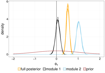
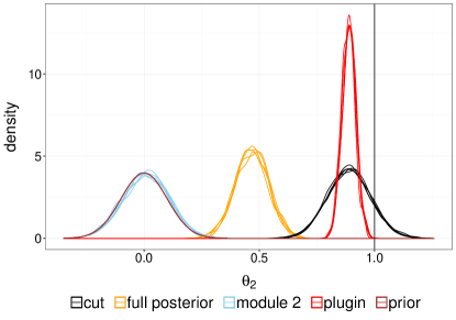
Figure 2: Various candidate distributions for $\theta_{1}$ (left) and $\theta_{2}$ (right), in the biased data example of Section 4.1. The data-generating values are indicated by vertical black lines.

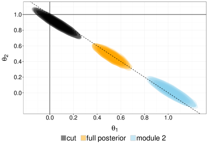
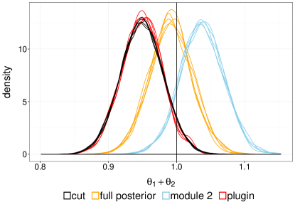
Figure 3: Cut distribution, full posterior and posterior in the second module, in the biased data example of Section 4.1. Joint distribution on the left, and marginal distribution of $\theta_{1}+\theta_{2}$ on the right. The data-generating values are indicated by black lines. On the left, the diagonal dashed line indicates the set of parameters such that $\theta_{1}+\theta_{2}=1$, which are optimal for prediction.

4.2 Epidemiological study

Plummer (2014) describes a simple and reproducible example inspired by epidemiological studies, and in particular by an investigation of the international correlation between human papillomavirus (HPV) prevalence and cervical cancer incidence (Maucort-Boulch et al., 2008). The focus of Plummer (2014) is on computational challenges with the cut distribution (see Section 5), while we use the example to test whether our proposed method selects the full posterior or the cut distribution.

In the toy version of the model, the first module specifies HPV prevalence, independently for datasets collected in $13$ countries. The parameter $\theta_{1}=\theta_{1,1:13}$ has prior distribution $\theta_{1,i}\sim\text{Beta}(1,1)$, independently for all $1\leq i\leq 13$. The data $Y_{1}^{1:13}$ are $13$ pairs of integers, the first being the number of women infected with high-risk HPV, and the second being a population size; we write $Y_{1}^{i}=(Y_{1}^{i}[1],Y_{1}^{i}[2])$ for all $1\leq i\leq 13$. The likelihood specifies that the data are independent across countries and that $Y_{1}^{i}[1]\sim\text{Binomial}(Y_{1}^{i}[2],\theta_{1,i})$ for all $1\leq i\leq 13$. By conjugacy, the posterior distribution factorizes into a product of Beta distributions, $\text{Beta}(1+Y_{1}^{i}[1],1+Y_{1}^{i}[2]-Y_{1}^{i}[1])$ for all $1\leq i\leq 13$.

The second module represents the relationship between HPV prevalence $\theta_{1}$ and cancer incidence, in the form of a Poisson regression. The parameters are $\theta_{2}=(\theta_{2,1},\theta_{2,2})$, both assumed to follow a Normal distribution $\mathcal{N}(0,10^{3})$, a priori. The second module specifies

$$\forall i\in\left\{1,\ldots,13\right\}\quad Y_{2}^{i}[1]\sim\text{Poisson}(\exp\left(\theta_{2,1}+\theta_{1,i}\theta_{2,2}+Y_{2}^{i}[2]\right)),$$

where the second dataset $Y_{2}^{1:13}$ is made of pairs $\left(Y_{2}^{i}[1],Y_{2}^{i}[2]\right)_{i=1}^{13}$ representing, respectively, the number of cancer incidents and the number of years at follow-up. It is suspected that the Poisson regression might be misspecified, and Plummer (2014) discusses computational methods to approximate the cut distribution. Note that the first parameters are the covariates in the regression specified by the second module. Therefore, the parameters have no clear interpretation if the second module is considered on its own: one would not typically consider both covariates and regression coefficients to be unknown simultaneously.

Some of the marginal distributions of $\theta_{1}$ are shown in Figure 4. The full posterior is in agreement with the first module’s posterior for some parameters (such as $\theta_{1,1}$) but not for others (such as $\theta_{1,9}$). The posterior in the second module is in disagreement with the full posterior and the first module’s posterior on most parameters. We show the bivariate candidate distributions for $(\theta_{2,1},\theta_{2,2})$, and the marginal distributions of $\theta_{2,2}$ in Figure 5. We see that the plug-in and the cut distributions give similar estimates for $\theta_{2,2}$, but the cut distribution is more diffuse. Furthermore, it overlaps very little with the full posterior distribution, so that decisions derived from the cut approach would likely be different.

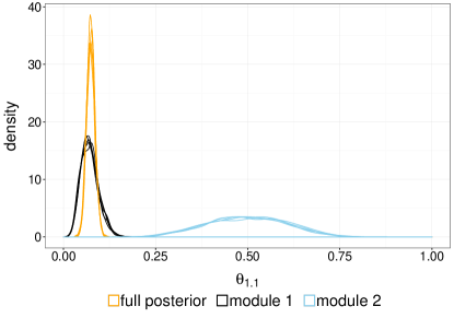
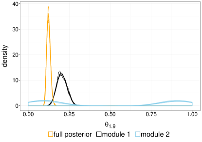
Figure 4: Various candidate distributions for $\theta_{1,1}$ (left) and $\theta_{1,9}$ (right), in the epidemiological study of Section 4.2. The full posterior is in agreement with the first module’s posterior for some parameters (such as $\theta_{1,1}$) but not for others (such as $\theta_{1,9}$).

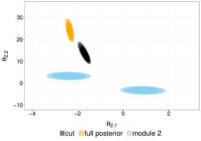
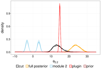
Figure 5: Various candidate distributions for $(\theta_{2,1},\theta_{2,2})$ (left) and marginal distribution of $\theta_{2,2}$ (right), in the epidemiological study of Section 4.2. The candidates overlap very little with one another. Based on the predictive performance of $\theta_{1}$ in terms of predicting $Y_{1}$, the cut distribution could be preferred, even though it yields a lower predictive score for $Y_{2}$ than the full posterior or the posterior in the second module only.

The predictive scores are given in Table 2. If we consider the task of predicting $Y_{1}$, we find that the full model has worse predictive performance than the first module on its own, but better predictive performance than the second module on its own. This indicates that $Y_{2}$ does not help in predicting $Y_{1}$. In this example, with only one observation per study, the prior predictive performance in the first module corresponds to the prequential predictive performance. In terms of parameter estimation, following our plan of action (Section 2.4), we would use the first module on its own to estimate $\theta_{1}$, and the cut distribution to estimate $(\theta_{1},\theta_{2})$, since it is the only candidate considered with $\bar{\pi}(\theta_{1}|Y_{1})$ as its first marginal.

If we consider the task of predicting $Y_{2}$, we find that the full model has worse predictive performance than the second module on its own. The cut approach yields a lower score, and finally the plug-in approach yields the lowest score. As in the previous section, the cut distribution is selected by our plan of action even though its predictions for $Y_{2}$ yield a lower score than the predictions under the full posterior.

	predictive score on $Y_{1}$
module 1	-64.8 [-65, -64.7]
full model	-74.9 [-75.1, -74.5]
module 2	-262.7 [-276.6, -253.5]

	predictive score on $Y_{2}$
module 2	11289 [11288.9, 11289.1]
full model	11285.1 [11285, 11285.2]
cut approach	11176 [11147.6, 11218.2]
plug-in approach	10836.2 [10836.1, 10836.3]

Table 2: Predictive performance of various candidates in the epidemiological study of Section 4.2, in terms of predicting $Y_{1}$ (left) and predicting $Y_{2}$ (right). The numbers represent the average score over $5$ Monte Carlo runs, with minimum and maximum values in brackets.

4.3 Propensity score

The propensity score methodology is used for causal inference in non-randomized experiments (Rosenbaum and Rubin, 1984). We will consider the setting of Zigler (2016) where the defects of the full posterior are explained in details. We use the example to test whether the proposed procedure favors modular approaches in an automatic, data-driven way.

We consider the effect of a variable $X$ (e.g. $X=1$ if “exposure to a treatment”, $X=0$ otherwise) on an outcome $Z$ (e.g. $Z=1$ if some event happens, $Z=0$ otherwise), for a number of individuals $i\in\left\{1,\ldots,n\right\}$. We have access to other covariates $C\in\mathbb{R}^{n\times p}$, which might be correlated with both $X$ and $Z$ since the experiment was not randomized. An attempt at correcting for confounding effects goes as follows. First perform a logistic regression of $X$ on the covariates $C$,

$$\forall i\in\{1,\ldots,n\}\quad\text{logit}\,\mathbb{P}\left(X_{i}=1\mid C_{i}\right)=\theta_{1,0}+\sum_{j=1}^{p}\theta_{1,j}C_{ij},$$ (11)

where $C_{i}$ denotes the $i$-th row of $C$. The quantity $e_{i}=\mathbb{P}\left(X_{i}=1\mid C_{i}\right)$ is referred to as the propensity score of individual $i$, and is a scalar summary of the relationship between the covariates and the treatment variable. For our purposes, the above logistic regression defines a first module with parameters $\theta_{1}=(\theta_{1,0},\ldots,\theta_{1,p})$, on which a centered Normal prior distribution is specified. The prior variance is set to $800$ on the intercept and to $50$ for the other coefficients.

One can proceed to the regression of $Z$ on $X$ over groups of individuals that share similar propensity scores. We consider a stratification of the scores $e_{i}$ in quintiles; the variable $q_{i}\in\left\{1,\ldots,5\right\}$ for each $i\in\{1,\ldots,n\}$ indicates to which quintile each $e_{i}$ belongs. The vector $q$ is deterministic given $e$, and thus deterministic given $\theta_{1}$, $X$ and $C$. The effect of $X$ on $Z$ can be modelled with another a logistic regression,

$$\forall i\in\{1,\ldots,n\}\quad\text{logit}\,\mathbb{P}\left(Z_{i}=1\mid X_{i},q_{i}\right)=\theta_{2,0}+\theta_{2,1}X_{i}+\sum_{k=2}^{5}\theta_{2,k}\delta_{k}\left(q_{i}\right),$$ (12)

where $\delta_{k}(q_{i})$ is equal to $1$ if $q_{i}=k$, and $0$ otherwise. Along with a Normal prior on $\theta_{2}=(\theta_{2,0},\ldots,\theta_{2,5})$, centered at zero and with variance $800$ on the intercept and $50$ on the other coefficients, this concludes the specification of the second module. The object of interest might be the parameter $\theta_{2,1}$ (or by-products of it), which is the coefficient of the treatment variable in the above logistic regression.

Standard practice in this setting is to obtain the propensity scores $e_{i}$ from the first module only, and to plug them into the second module to estimate $\theta_{2,1}$. Indeed, the goal of the propensity score approach is to compensate for lack of randomization in the experiment. In a randomized experiment, the assignment of $X$ is, by design, independent of the covariates $C$, and the outcome $Z$ would not be observed at the time when $X$ is assigned. Therefore, it seems odd to use the outcome variable $Z$ in order to estimate propensity scores that relate to the treatment assignment part of the problem. However, if we do have access to $Z$ from the onset, it is legitimate to wonder whether it should be used in the estimation of propensity scores. A series of interesting articles (Zigler et al., 2013; Zigler and Dominici, 2014; Zigler, 2016) investigates this question. We consider the experiment described in Zigler (2016), where $n=1000$ individuals have $p=6$ covariates, generated as independent Normal realizations: $C_{ij}\sim\mathcal{N}(0,1)$ for all $i,j$. The treatment variable $X_{i}\in\{0,1\}$ is generated according to a logistic regression:

$$\forall i\in\{1,\ldots,n\}\quad\text{logit}\,\mathbb{P}\left(X_{i}=1\mid C_{i}\right)=\theta_{1,0}^{\star}+\sum_{j=1}^{6}\theta_{1,j}^{\star}C_{ij},$$

where $\theta_{1}^{\star}=(0,0.1,0.2,0.3,0.4,0.5,0.6)$: the first module is well-specified. Given $X$ and $C$, we generate an outcome variable $Z$ via the equation

$$\forall i\in\{1,\ldots,n\}\quad\text{logit}\mathbb{P}\left(Z_{i}=1\mid X_{i},C_{i}\right)= \gamma_{1}^{\star}C_{i1}+\gamma_{2}^{\star}\exp\left(C_{i2}-1\right)$$

$$+\gamma_{3}^{\star}C_{i3}+\gamma_{4}^{\star}\exp\left(C_{i4}-1\right)+\gamma_{5}^{\star}|C_{i5}|+\gamma_{6}^{\star}|C_{i6}|,$$

where $\gamma^{\star}=(0.6,0.5,0.4,0.3,0.2,0.1)$: the second module is misspecified. One question is whether the model can be used to investigate causal effects of $X$ on $Z$, despite that misspecification. Here, given the covariates $C$, the outcome $Z$ is generated independently of $X$, so that we hope that a statistical approach to causal inference would conclude at an absence of causal effect of $X$ on $Z$: in other words, we want to estimate $\theta_{2,1}$ close to zero.

Some marginal distributions of $\theta_{1}$ are shown in Figure 6. The posterior under the second module only yields a very flat distribution on the regression parameters, omitted from the plots for clarity. As in Section 4.2, we would not expect users to consider the posterior given $Z$ alone, as the propensity scores would then result from prior information only, but we include the associated score in the tables, to emphasize that it would yield the best predictive performance for $Z$. In Figure 6 we see that the first posterior puts its mass near the data-generating values, whereas the full posterior is sometimes in disagreement, e.g. for $\theta_{1,1}$.

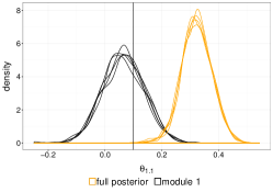
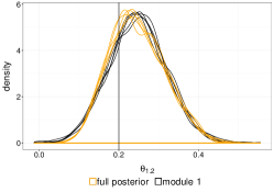
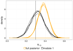
Figure 6: Distribution of some regression coefficients in the first module, in the propensity score example of Section 4.3. The values used to generate the data are indicated by vertical black lines.

Some candidates distributions for $\theta_{2,1}$ are displayed in Figure 7. The absence of causal effect of $X$ on $Z$ can indeed be retrieved from either the cut and the plug-in distributions, the expectations of which are close to zero. The full posterior is shifted towards negative values, while the posterior in the second module puts more mass on positive values.

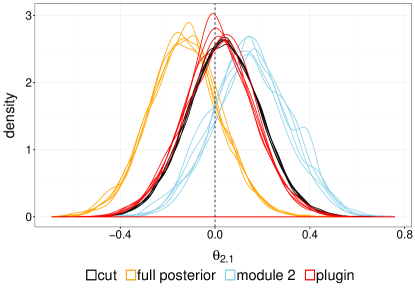
Figure 7: Distribution of $\theta_{2,1}$, the coefficient of $X$ in the regression of $Z$ on $X$ and the propensity score quintile indicators, in the propensity score example of Section 4.3. The vertical dashed line at zero indicates that we expect to retrieve zero as the result of the inference, since the values of $Z$ are generated irrespectively of the values of $X$.

Table 3 contains the predictive scores. For this example, our proposed plan of action again leads to modular approaches over the full posterior. For $\theta_{1}$, looking at the predictive performance for $Y_{1}$, we would use the first module posterior. To preserve $\pi_{1}(\theta_{1}|X,C)$ as the first marginal of a distribution on $(\theta_{1},\theta_{2})$, we would choose the cut distribution, even though it yields lower predictive scores for $Y_{2}$. This experiment illustrates again that modular approaches favored by practitioners can be validated by quantitative criteria, and that the full posterior can underperform in the presence of misspecification.

	predictive score on $X$
module 1	-632.9 [-633.1, -632.7]
full model	-664.4 [-665.5, -663.4]
prior	-694.4 [-695.6, -693.1]
module 2	-6775.7 [-8422.4, -5351]

	predictive score on $Z$
module 2	-624 [-624.5, -623.6]
full model	-646.2 [-646.3, -646.1]
cut approach	-648.7 [-650.3, -647]
plug-in approach	-652.4 [-652.5, -652.3]

Table 3: Predictive performance of various candidates in the propensity score example of Section 4.3, in terms of predicting $X$ in the first module (left) and predicting $Z$ in the second one (right). The numbers represent the average score over $5$ Monte Carlo runs, with minimum and maximum values in brackets.

4.4 Meta-analysis

Here we go beyond models made of two modules, to illustrate how the proposed procedure can be adapted in other settings. Calculations are provided in Appendix A.

4.4.1 Model and candidate distributions

This example is again taken from Liu et al. (2009), where it raises concerns about the full posterior in certain hierarchical models. We use the example to test whether the defects of the full posterior can be detected automatically with the proposed approach. Consider $N$ studies, indexed by $i\in 1:N$, and $n_{i}$ individuals in each study $i$, indexed by $j\in 1:n_{i}$. The entire data set is denoted by $y=(y_{i,j})$, and the data of study $i$ by $y_{i}=(y_{i,1},\ldots,y_{i,n_{i}})$. The average of the observations in study $i$ is $\bar{y}_{i}=n_{i}^{-1}\sum_{j=1}^{n_{i}}y_{i,j}$ and we also introduce $s_{i}^{2}=\sum_{j=1}^{n_{i}}\left(y_{i,j}-\bar{y}_{i}\right)^{2}$. The model specifies, for all $i\in 1:N$ and all $j\in 1:n_{i}$, that the observation $y_{i,j}$ follows the distribution $\mathcal{N}(b_{i},\sigma_{i}^{2})$, where $\sigma_{i}^{2}$ here denotes the variance. The prior distribution on $(b_{i},\sigma_{i}^{2})$ for all $i\in 1:N$ and on $\tau^{2}$ is specified as

$$b_{i}\sim\mathcal{N}(0,\tau^{2}),\quad p(\sigma_{i}^{2})\propto\frac{1}{\sigma_{i}^{2}},\quad p(\tau^{2}|\sigma_{1:N}^{2})\propto\frac{1}{\tau^{2}+N^{-1}\sum_{i=1}^{N}(\sigma_{i}^{2}/n_{i})}.$$ (13)

The above is a reference prior according to Liu et al. (2009). The link between the studies is the variance parameter $\tau^{2}$. The posterior distribution of $\sigma_{i}^{2}$ given $\tau^{2}$ in study $i\in 1:N$, integrating $b_{i}$ out, is given by

$$p(\sigma_{i}^{2}|\tau^{2},y_{i})\propto\frac{\sigma_{i}^{-n_{i}-1}}{\sqrt{\tau^{2}+\sigma_{i}^{2}/n_{i}}}\exp\left(-\frac{1}{2}\frac{\left(\bar{y}_{i}\right)^{2}}{\left(\tau^{2}+\sigma_{i}^{2}/n_{i}\right)}-\frac{s_{i}^{2}}{2\sigma_{i}^{2}}\right).$$ (14)

This leads to the full posterior of $\tau^{2},\sigma_{1:N}^{2}$ given $y$:

$$p(\tau^{2},\sigma_{1:N}^{2}|y) \propto\frac{1}{\tau^{2}+N^{-1}\sum_{i=1}^{N}(\sigma_{i}^{2}/n_{i})}\prod_{i=1}^{N}\frac{\sigma_{i}^{-n_{i}-1}}{\sqrt{\tau^{2}+\sigma_{i}^{2}/n_{i}}}\exp\left(-\frac{1}{2}\frac{\left(\bar{y}_{i}\right)^{2}}{\left(\tau^{2}+\sigma_{i}^{2}/n_{i}\right)}-\frac{s_{i}^{2}}{2\sigma_{i}^{2}}\right).$$ (15)

We can evaluate the above expression for all non-negative values of $\tau^{2},\sigma_{1:N}^{2}$, and thus we can perform Markov chain Monte Carlo (MCMC) to approximate the full posterior $p(\tau^{2},\sigma_{1:N}^{2}|y)$. Finally, given $(\tau^{2},\sigma_{1:N}^{2},y)$, the conditional distribution of $b_{i}$ is given by:

$$b_{i}\sim\mathcal{N}\left(\frac{\bar{y}_{i}\tau^{2}}{\tau^{2}+\sigma_{i}^{2}/n_{i}},\frac{\tau^{2}\sigma_{i}^{2}/n_{i}}{\tau^{2}+\sigma_{i}^{2}/n_{i}}\right).$$ (16)

In Liu et al. (2009), the cut distribution is introduced as follows. The conditional distribution of $\tau^{2}$ given $(\sigma_{1:N}^{2},y)$ is that of the full posterior (dropping constants in $\tau^{2})$:

$$p(\tau^{2}|\sigma_{1:N}^{2},y)\propto\frac{1}{\tau^{2}+N^{-1}\sum_{i=1}^{N}(\sigma_{i}^{2}/n_{i})}\prod_{i=1}^{N}\frac{\sigma_{i}^{-n_{i}-1}}{\sqrt{\tau^{2}+\sigma_{i}^{2}/n_{i}}}\exp\left(-\frac{1}{2}\frac{\left(\bar{y}_{i}\right)^{2}}{\left(\tau^{2}+\sigma_{i}^{2}/n_{i}\right)}\right),$$ (17)

with an intractable normalizing constant that is a function of $\sigma_{1:N}^{2}$. The marginal distribution of $\sigma_{1:N}^{2}$ given $y$ is specified as

$$p^{\text{cut}}(\sigma_{1:N}^{2}|y)=\prod_{i=1}^{N}p(\sigma_{i}^{2}|y_{i})\propto\prod_{i=1}^{N}\sigma_{i}^{-n_{i}-1}\exp\left(-\frac{s_{i}^{2}}{2\sigma_{i}^{2}}\right),$$ (18)

which is a product of Inverse Gamma densities. This is defined as long as $n_{i}\geq 2$ for all $i\in 1:N$. The joint cut distribution of $(\tau^{2},\sigma_{1:N}^{2})$ is the product of the marginal of Eq. (18) and the conditional of Eq. (17):

$$p^{\text{cut}}(\tau^{2},\sigma_{1:N}^{2})=p(\tau^{2}|y,\sigma_{1:N}^{2})p^{\text{cut}}(\sigma_{1:N}^{2}|y).$$ (19)

Because of the intractable normalizing constant in $p(\tau^{2}|y,\sigma_{1:N}^{2})$, we cannot directly perform MCMC to approximate $p^{\text{cut}}(\tau^{2},\sigma_{1:N}^{2})$. The constant could be accurately approximated, since it is the integral of the right-hand side of Eq. (17) with respect to $\tau^{2}$, which is a one-dimensional variable. We will prefer the following procedure that generates i.i.d. draws from the cut distribution.

We can obtain i.i.d. samples from $p^{\text{cut}}(\sigma_{1:N}^{2}|y)$ by inverting Gamma variables, and then sample $\tau^{2}$ given such draws, using rejection sampling. To this aim, we perform a reparametrization of $\tau^{2}$, introducing $u=(1+\tau^{2})^{-1}$, with inverse $\tau^{2}=u^{-1}-1$. Applying that change of variable to Eq. (17), the distribution of $u$ given $(\sigma_{1:N}^{2},y)$ has density proportional to

$$\frac{1}{u^{-1}-1+N^{-1}\sum_{i=1}^{N}(\sigma_{i}^{2}/n_{i})}\prod_{i=1}^{N}\frac{\sigma_{i}^{-n_{i}-1}}{\sqrt{u^{-1}-1+\sigma_{i}^{2}/n_{i}}}\exp\left(-\frac{1}{2}\frac{\left(\bar{y}_{i}\right)^{2}}{\left(u^{-1}-1+\sigma_{i}^{2}/n_{i}\right)}\right)\times\left|\frac{1}{u^{2}}\right|.$$

The maximum value of the above expression, over all $u\in[0,1]$, can be obtained numerically, which enables rejection sampling; we will use a Uniform distribution on $[0,1]$ as a proposal distribution.

4.4.2 The issue with the full posterior

We illustrate the issue with the full posterior and the appeal of the cut distribution in a numerical experiment inspired by the discussion in Liu et al. (2009) about the defects of the full posterior distribution in misspecified random-effects models.

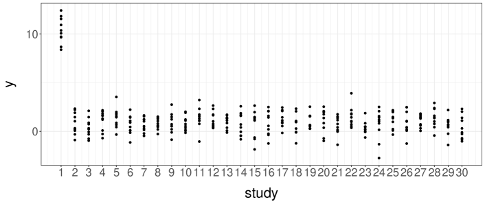
Figure 8: Data generated from the meta-analysis model of Section 4.4, with $b_{1}^{\star}=10$, $b_{i}^{\star}=1$ for $i\in 2:N$ and $\sigma_{i}^{\star}=1$ for $i\in 1:N$, with $N=30$ studies and $n_{i}=10$ individuals per study.

We set $N=30$ and $n_{i}=10$ for all $i\in 1:N$. The data-generating parameters are set to $b_{1}^{\star}=10$, $b_{i}^{\star}=1$ for $i\in 2:N$, and $\sigma_{i}^{\star}=1$ for all $i\in 1:N$. The data are shown in Figure 8. We obtain the parameters $(\tau,\sigma_{1:N},b_{1:N})$ given the data under both the full posterior distribution and the cut approach. The marginal distributions of $(\sigma_{1},b_{1})$ and $(\sigma_{2},b_{2})$ are shown in Figure 9. The marginals of $(\sigma_{i},b_{i})$ for $i\in 3:N$ are similar to that of $(\sigma_{2},b_{2})$, and are thus not shown. The horizontal and vertical dashed lines indicate the values of $b_{i}^{\star}$ and $\sigma_{i}^{\star}$. From the plots, it is apparent that the distribution obtained with the cut approach is more able to retrieve the data-generating values. Note the bimodality of the full posterior distribution of $(\sigma_{1},b_{1})$, with a minor mode located where the cut distribution puts most of its mass. The marginal distribution of $(\tau,\sigma_{1})$ is also shown, and also features two modes. From the numerical experiments, the cut distribution puts most of its mass close to the data-generating values $b_{1}^{\star},\sigma_{1}^{\star}$, whereas the full posterior distribution does not.

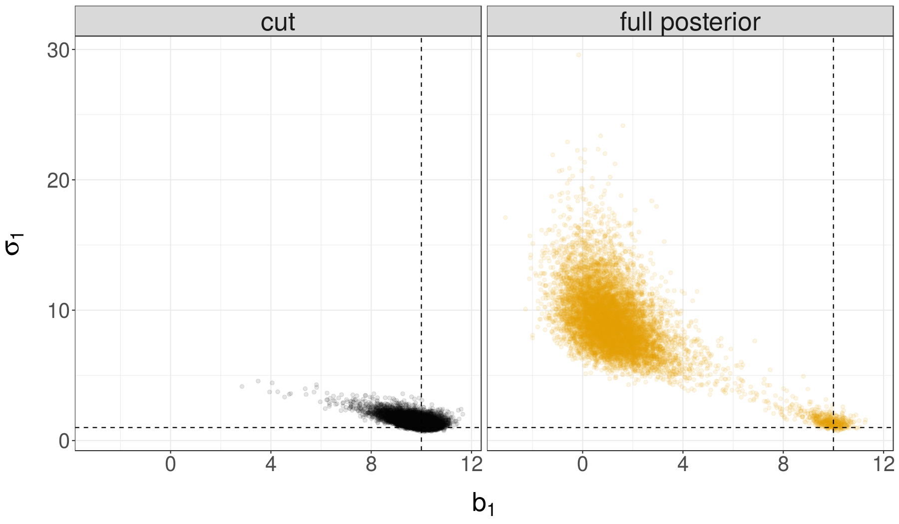
(a) Marginal distribution of $(b_{1},\sigma_{1})$.

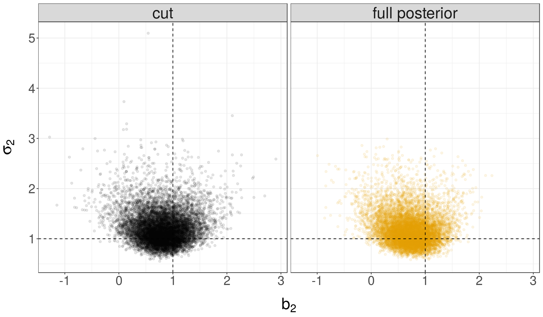
(b) Marginal distribution of $(b_{2},\sigma_{2})$.

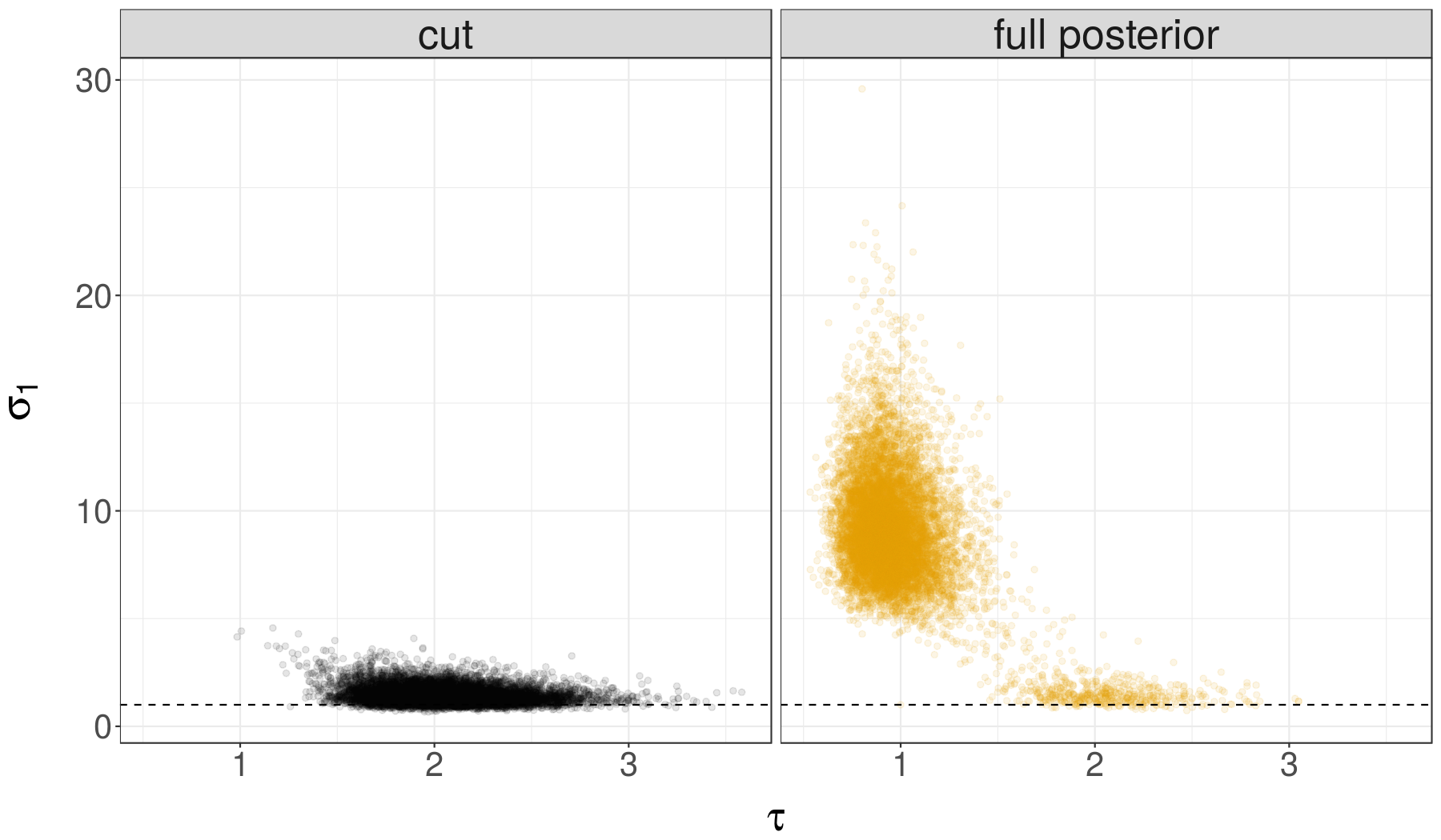
(c) Marginal distribution of $(\tau,\sigma_{1})$.

Figure 9: Marginal posterior distributions of $(b_{1},\sigma_{1})$, $(b_{2},\sigma_{2})$ (top and middle row), and of $(\tau,\sigma_{1})$ (bottom row) under the full model posterior and the cut distribution in the meta-analysis example of Section 4.4. The distributions of $(b_{i},\sigma_{i})$ for $i\in 3:n$ are similar to that of $(b_{2},\sigma_{2})$, and thus not shown.

4.4.3 Predictive criteria

We are now interested in a data-driven predictive criterion to decide between the full posterior and the cut approach, without knowledge of the data-generating values $b_{1:N}^{\star},\sigma_{1:N}^{\star}$. In the present context, several obstacles appear in the way of our proposed plan of action.

• The number of observations, $n_{i}$ in study $i$, enters the specification of the prior distribution. Therefore, the task of sequential prediction is ambiguous: either we specify the prior once and for all, using $n_{i}$ in study $i$, or we redefine the prior sequentially as we assimilate more and more observations, replacing $n_{i}$ in the prior by the current number of observations. We choose to fix $n_{i}$ in the prior specification, even when we predict $y_{i,j}$ given $y_{i,1:j-1}$ for $j<n_{i}$.

• The prior is improper, and the cut distribution is well-defined only if $n_{i}\geq 2$ for any $i\in 1:N$.

• We can either define a single criterion quantifying the quality of the predictions of all observations, or we can define a criterion for each study, quantifying the predictive quality conditional upon the data of the other studies. We choose the latter, enabling the identification of problematic studies.

We now describe the proposed study-specific predictive criterion. For a study $i\in 1:N$, denote by $y_{\setminus i}$ the data of the other studies, and $\sigma_{\setminus i}^{2}$ denotes $\sigma_{i^{\prime}}^{2}$ for all $i^{\prime}\neq i$. For the task of predicting the observations $y_{i,j}$, for $j\in 1:n_{i}$, given $y_{\setminus i}$ and $y_{i,1},\ldots,y_{i,j-1}$, we will condition on the first two observations, $y_{i,1},y_{i,2}$, otherwise the cut distribution in Eq. (19) would not be defined. We introduce a predictive criterion under the full posterior approach before introducing a comparable criterion for the modularized approach.

First, we obtain a sample approximating the distribution of $(\tau^{2},\sigma_{1:N}^{2})$ given $(y_{\setminus i},y_{i,1},\ldots,y_{i,j})$, as in Eq. (15), using only $j$ observations, $y_{i,1:j}$, in the $i$-th study; we still use $n_{i}$ in the definition of the prior distribution of $\tau^{2}$ conditional on $\sigma_{1:N}^{2}$. We then proceed to computing, for all $j\in\{3,\ldots,n_{i}\}$,

$$p(y_{i,j}|y_{\setminus i},y_{i,1},\ldots,y_{i,j-1})=\int p(y_{i,j}|\sigma_{i}^{2},\tau^{2},y_{i,1},\ldots,y_{i,j-1})p(\tau^{2},\sigma_{\setminus i}^{2},\sigma_{i}^{2}|y_{\setminus i},y_{i,1},\ldots,y_{i,j-1})d\tau^{2}d\sigma_{1:N}^{2},$$ (20)

where we can approximate the integral by Monte Carlo samples. Note that we can either do this for each $j\in\{3,\ldots,n_{i}\}$, independently, or we can use a sequential Monte Carlo sampler, starting from the distribution of $(\tau^{2},\sigma_{1:N}^{2})$ given $(y_{\setminus i},y_{i,1:2})$ and assimilating $y_{i,3:n_{i}}$ one by one. We then aggregate the predictive scores of each observation, leading to the criterion

$$\log p(y_{i,3:n_{i}}|y_{\setminus i},y_{i,1:2})=\sum_{j=3}^{n_{i}}\log p(y_{i,j}|y_{\setminus i},y_{i,1},\ldots,y_{i,j-1}),$$

which is quantity that would also appear in a partial Bayes factor (O’Hagan, 1995; Berger and Pericchi, 1996). Since the ordering of the observations in each study is arbitrary, we could average the above criterion over the “2 choose $n_{i}$” choices of first two observations, at the cost of more calculations.

Under the cut approach, we define similarly, for all $j\in\{3,\ldots,n_{i}\}$,

$$p^{\text{cut}}(y_{i,j}|y_{\setminus i},y_{i,1},\ldots,y_{i,j-1}) =\int p(y_{i,j}|\sigma_{i}^{2},\tau^{2},y_{i,1},\ldots,y_{i,j-1})p^{\text{cut}}(\tau^{2},\sigma_{\setminus i}^{2},\sigma_{i}^{2}|y_{\setminus i},y_{i,1},\ldots,y_{i,j-1})d\tau^{2}d\sigma_{1:N}^{2},$$

$$\log p^{\text{cut}}(y_{i,3:n_{i}}|y_{\setminus i},y_{i,1:2}) =\sum_{j=3}^{n_{i}}\log p^{\text{cut}}(y_{i,j}|y_{\setminus i},y_{i,1},\ldots,y_{i,j-1}),$$

and again, we could average over permutations of $y_{i,1:n_{i}}$ at the cost of extra calculations.

The two quantities $\log p(y_{i,3:n_{i}}|y_{\setminus i},y_{i,1:2})$ and $\log p^{\text{cut}}(y_{i,3:n_{i}}|y_{\setminus i},y_{i,1:2})$ can then be compared for each study $i$. Indeed, they monitor the performance of sequential probabilistic predictions of the same observations, under the same logarithmic scoring rule. Figure 10 shows the predictive criterion for each study, approximated by $10$ independent Monte Carlo runs. The mean plus and minus two standard deviations of these $10$ runs are shown in error bars. It is apparent that the predictive power of the cut approach is higher for the first study. For the other studies, the cut approach and the full posterior give mostly comparable results. The graph helps identifying which study is problematic for the full posterior approach.

Figure 10: Prediction criterion for each study given the others, in the meta-analysis model, under the cut approach and the full posterior. The error bars show the mean plus and minus two standard errors, of criteria computed $10$ times independently, using Monte Carlo methods.

5 Computational challenges

In this section, we explain how the tables and figures of Section 4 were obtained, and the associated computational challenges. We first discuss algorithms to sample distributions and to estimate their normalizing constants (Section 5.1). We then discuss the challenges associated with the cut distribution (Section 5.2). Finally, we revisit computational issues in the context of data confidentiality (Section 5.3).

5.1 Sampling distributions and estimating their normalizing constants

We assume that the prior density and the likelihood can be evaluated for each parameter, up to a multiplicative constant, in both modules. Generic Monte Carlo algorithms can be used to obtain draws from various candidate distributions, such as $\bar{\pi}(\theta_{1}|Y_{1})$ or $\bar{\pi}(\theta_{1},\theta_{2}|Y_{1},Y_{2})$. In order to compare modular approaches, we require estimates of the associated predictive scores, such as $\log\bar{\pi}(Y_{1})$ in the first module, or $\log\bar{\pi}(Y_{1}|Y_{2})$ in the full model. These scores correspond to logarithms of normalizing constants in Bayes’ formula, e.g. $\bar{\pi}(\theta_{1}|Y_{1})=p_{1}(\theta_{1})p(Y_{1}|\theta_{1})/\bar{\pi}(Y_{1})$, $\bar{\pi}(\theta_{1},\theta_{2}|Y_{1},Y_{2})=\bar{\pi}(\theta_{1},\theta_{2}|Y_{2})p_{1}(Y_{1}|\theta_{1})/\bar{\pi}(Y_{1}|Y_{2})$. Importance sampling and sequential Monte Carlo (SMC) samplers (Chopin, 2002; Del Moral et al., 2006) approximate posterior distributions and estimate their normalizing constants jointly. Theoretical works provide support and insight on their precision as a function of their computational cost (Schweizer, 2012; Whiteley, 2012; Beskos et al., 2014a, b), and SMC samplers have been shown to compare favorably to other normalizing constant estimation techniques in Zhou et al. (2016). Details on the adaptive SMC sampler used in all experiments are given in Appendix B.

5.2 Sampling from the cut distribution

The approximation of the cut distribution $\pi^{\text{cut}}(\theta_{1},\theta_{2}|Y_{1},Y_{2})$ and its predictive score, as in Eq. (9), can also be done with SMC samplers, in two stages. First, one obtains a sample $\Theta_{1}^{1:N}$ approximating $\bar{\pi}(\theta_{1}|Y_{1})$. To approximate the predictive score of the cut approach, one can approximate each term in the sum of Eq. (9),

$$\log(\int p_{2}(Y_{2}^{i}|\theta_{1},\theta_{2})\bar{\pi}(\theta_{1}|Y_{1})\bar{\pi}(\theta_{2}|\theta_{1},Y_{2}^{1:i-1})d\theta_{1}d\theta_{2}),$$

for $1\leq i\leq n_{2}$, by the Monte Carlo approximation $\log(N^{-1}\sum_{k=1}^{N}\bar{\pi}(Y_{2}^{i}|\Theta_{1}^{k},Y_{2}^{1:i-1}))$. The terms $\bar{\pi}(Y_{2}^{i}|\Theta_{1}^{k},Y_{2}^{1:i-1})$, for $1\leq i\leq n_{2}$ can be approximated, for each $\Theta_{1}^{k}$, $1\leq k\leq N$, again by Monte Carlo. This yields a sample $\Theta_{2,i-1}^{k,1:M}$ approximating $\bar{\pi}(\theta_{2}|\Theta_{1}^{k},Y_{2}^{1:i-1})$, for some integer $M$ chosen by the user. One can prune these samples to obtain one value $\Theta_{2,i-1}^{k}$, for each $k$; the resulting pairs $(\Theta_{1}^{k},\Theta_{2,i-1}^{k})_{k=1}^{N}$ approximate the joint cut distribution given $Y_{1}$ and $Y_{2}^{1:i-1}$. Iterating through the data $Y_{2}^{1},\ldots,Y_{2}^{n_{2}}$ yields approximations of the sequence of cut distributions and of the cut score of Eq. (9).

The above procedure can be considered naive since it involves running a Monte Carlo method for each value $\Theta_{1}^{k}$ obtained in the approximation of $\bar{\pi}(\theta_{1}|Y_{1})$. Although these runs can be done in parallel, it raises the question of whether a sampling approach targeting the cut distribution is possible in one stage. Plummer (2014) discusses the problem of designing Markov kernels leaving $\pi^{\text{cut}}(\theta_{1},\theta_{2}|Y_{1},Y_{2})$ invariant, and notes that previous attempts have resulted in incorrect samplers. The main difficulty lies in the intractability of the term $\bar{\pi}(Y_{2}|\theta_{1})$ in Eq. (5), which involves an integral over $\theta_{2}$. An alternative way of approximating the cut distribution is proposed in Jacob et al. (2017).

5.3 Two-stage Monte Carlo approaches in confidential settings

A two-stage Monte Carlo approach, such as that described in the previous section, has practical advantages in a context of confidential data sets. For various reasons, the user might not have access simultaneously to $Y_{1}$ and $Y_{2}$, or even to both prior and likelihood functions. Consider the scenario where one is given draws $\Theta_{1}^{1:N}$ from some distribution $\bar{\pi}(\theta_{1}|Y_{1})$, which could be the posterior in a first module, and one wants to consider modular and full approaches for a second module. The cut distribution and its predictive score can be approximated via the above SMC procedures. Can one retrieve the full posterior distribution $\bar{\pi}(\theta_{1},\theta_{2}|Y_{1},Y_{2})$, without further access to the first module?

As described above, algorithms such as SMC samplers provide $\Theta_{2,i}^{k}$ approximately from $\bar{\pi}(\theta_{2}|\Theta_{1}^{k},Y_{2}^{1:i})$, as well as estimates $\hat{\pi}^{M}(Y_{2}^{i}|\Theta_{1}^{k},Y_{2}^{1:i-1})$ of the terms $\bar{\pi}(Y_{2}^{i}|\Theta_{1}^{k},Y_{2}^{1:i-1})$, for all $1\leq i\leq n_{2}$. This enables an importance sampling scheme, where the proposal distribution is $\pi^{\text{cut}}(\theta_{1},\theta_{2}|Y_{1},Y_{2}^{1:i})$ and the target distribution is $\bar{\pi}(\theta_{1},\theta_{2}|Y_{1},Y_{2}^{1:i})$, for any $1\leq i\leq n_{2}$. The importance weight function is the ratio of these densities, proportional $\bar{\pi}(Y_{2}^{1:i}|\theta_{1})$ for all $\theta_{1},\theta_{2}$, as can be seen from Eq. (5). Therefore, we can define the importance weights as $w_{i}^{k}=\hat{\pi}^{M}(Y_{2}^{1:i}|\Theta_{1}^{k})=\prod_{s=1}^{i}\hat{\pi}^{M}(Y_{2}^{s}|\Theta_{1}^{k},Y_{2}^{1:s-1})$, and normalize the weights as $W_{i}^{k}=w_{i}^{k}/\sum_{j=1}^{N}w_{i}^{j}$. The weighted samples $(W_{i}^{k},(\Theta_{1}^{k},\Theta_{2,i}^{k}))$, for $1\leq k\leq N$, approximate the distribution $\bar{\pi}(\theta_{1},\theta_{2}|Y_{1},Y_{2}^{1:i})$.

Furthermore, we can also approximate the predictive score $\log\bar{\pi}(Y_{2}|Y_{1})$, using the decomposition

$$\log\bar{\pi}(Y_{2}|Y_{1}) =\sum_{i=1}^{n_{2}}\log\bar{\pi}(Y_{2}^{i}|Y_{1},Y_{2}^{1:i-1})=\sum_{i=1}^{n_{2}}\log\left(\int p_{2}(Y_{2}^{i}|\theta_{1},\theta_{2})\bar{\pi}(\theta_{1},\theta_{2}|Y_{1},Y_{2}^{1:i-1})d\theta_{1}d\theta_{2}\right).$$

The integral on the right hand side can be approximated by the weighted samples introduced above. The idea of using Monte Carlo samples of a first distribution in an algorithm targeting a full posterior distribution can be found in Lunn et al. (2013), where the samples obtained in a first-stage MCMC chain are used as proposals in a second stage. The method of Lunn et al. (2013) could be applied here, but would not directly provide estimates of the normalizing constants, which are required for our proposed predictive scores.

The above approach is expected to work insofar as $\pi^{\text{cut}}(\theta_{1},\theta_{2}|Y_{1},Y_{2})$ is efficient enough as an importance sampling proposal for the target $\bar{\pi}(\theta_{1},\theta_{2}|Y_{1},Y_{2})$. In other words, the importance sampler will work if the feedback of $Y_{2}$ on $\theta_{1}$ is mild. Indeed a mild feedback implies that the first stage samples $\Theta_{1}^{1:N}$ already are a good approximation of the marginal of $\theta_{1}$ in the full posterior. On the other hand, if the feedback of $Y_{2}$ on $\theta_{1}$ is strong, approximating the marginal $\bar{\pi}(\theta_{1}|Y_{1},Y_{2})$ with samples from $\bar{\pi}(\theta_{1}|Y_{1})$ will likely fail. Figure 2 illustrates the potential mismatch between these distributions. In case of such mismatch, a sample $\Theta_{1}^{1:N}$ from the first module’s posterior does not spread enough over the support of the full posterior, which means that the prior $p_{1}(\theta_{1})$ and the likelihood $p_{1}(Y_{1}|\theta_{1})$ of the first module will have to be accessed again. This motivates the search for computational methods which would approximate the full posterior in two stages while querying the first module as rarely as possible.

6 Discussion

Combining task-specific data and models into coherent ensembles will be instrumental in the understanding of uncertainty in large-scale systems, arising in all fields: for instance, medical models of the human body and its organs (Dance, 2015), models of our planet and its climate systems (Shen et al., 2016), and models of ecosystems and their interacting species (Collie et al., 2016). How misspecified components should interact, and whether data can be used to derive optimal assemblies of components, will become pressing questions. In various settings, scientists have resorted to modular approaches to deal with misspecification while propagating uncertainties. We propose a principled and data-driven procedure to help deciding between modular and full inferential approaches, to make the best use of the available modules. As illustrated in the meta-analysis example in Section 4.4, the proposed criteria can be modified on a case-by-case basis to accommodate specificities, such as improper priors.

In numerical experiments, the proposed framework confirms that modular approaches outperform the full model posterior distribution in various settings, including meta-analysis and causal inference with propensity scores. The proposed plan of action relies on predictive scores, and on the selection of candidate distributions that yield the best predictions within the module that gives an interpretable meaning to the parameters, as described in Section 2.4.

Our proposed cut score depends on the ordering of the observations, which is potentially problematic; averaging over permutations of the data alleviates the issue but could be computationally expensive. Furthermore, the approximation of the cut distribution itself is challenging, as mainstream MCMC algorithms cannot be used, due to the intractability of the feedback term (Plummer, 2014; Jacob et al., 2017). Other modular approaches, such as those using power likelihoods mentioned in Section 3, would allow partial feedback of some modeling components on others; they would however raise their own computational challenges.

Appendix A Calculations for the meta-analysis example

To prove Eq. (14), we proceed as follows. By noting that

$$\sum_{j=1}^{n_{i}}\left(y_{i,j}-b_{i}\right)^{2}=\sum_{j=1}^{n_{i}}\left(y_{i,j}-\bar{y}_{i}\right)^{2}+n_{i}\left(\bar{y}_{i}-b_{i}\right)^{2},$$

we obtain

$$p(y_{i}|b_{i},\sigma_{i}^{2})=\left(2\pi\sigma_{i}^{2}\right)^{-n_{i}/2}\exp\left(-\frac{1}{2\sigma_{i}^{2}}\left(\sum_{j=1}^{n_{i}}\left(y_{i,j}-\bar{y}_{i}\right)^{2}+n_{i}\left(\bar{y}_{i}-b_{i}\right)^{2}\right)\right).$$

This leads to the posterior of $b_{i},\sigma_{i}^{2}$ given $\tau^{2}$ and $y_{i}$:

$$p(b_{i},\sigma_{i}^{2}|\tau^{2},y_{i})\propto\left(\sigma_{i}^{-2}\right)\sigma_{i}^{-n_{i}}\exp\left(-\frac{1}{2\sigma_{i}^{2}}\left(\sum_{j=1}^{n_{i}}\left(y_{i,j}-\bar{y}_{i}\right)^{2}+n_{i}\left(\bar{y}_{i}-b_{i}\right)^{2}\right)-\frac{1}{2\tau^{2}}b_{i}^{2}\right).$$ (21)

We can integrate $b_{i}$ out. Considering only the term in the exponential that features $b_{i}$, we note

$$\frac{n_{i}(\bar{y}_{i}-b_{i})^{2}}{\sigma_{i}^{2}}+\frac{b_{i}^{2}}{\tau^{2}} =\frac{n_{i}(\bar{y}_{i})^{2}-2b_{i}n_{i}\bar{y}_{i}+n_{i}b_{i}^{2}}{\sigma_{i}^{2}}+\frac{b_{i}^{2}}{\tau^{2}}$$

$$=(\frac{1}{\tau^{2}}+\frac{n_{i}}{\sigma_{i}^{2}})b_{i}^{2}-2\left(\frac{n_{i}\bar{y}_{i}}{\sigma_{i}^{2}}\right)b_{i}+\frac{n_{i}\left(\bar{y}_{i}\right)^{2}}{\sigma_{i}^{2}}$$

$$=(\frac{1}{\tau^{2}}+\frac{n_{i}}{\sigma_{i}^{2}})\left(b_{i}-\left(\frac{1}{\tau^{2}}+\frac{n_{i}}{\sigma_{i}^{2}}\right)^{-1}\left(\frac{n_{i}\bar{y}_{i}}{\sigma_{i}^{2}}\right)\right)^{2}-\left(\frac{1}{\tau^{2}}+\frac{n_{i}}{\sigma_{i}^{2}}\right)^{-1}\left(\frac{n_{i}\bar{y}_{i}}{\sigma_{i}^{2}}\right)^{2}+\frac{n_{i}\left(\bar{y}_{i}\right)^{2}}{\sigma_{i}^{2}}.$$

Write $\left(\frac{1}{\tau^{2}}+\frac{n_{i}}{\sigma_{i}^{2}}\right)^{-1}=\frac{\tau^{2}\sigma_{i}^{2}}{n_{i}\tau^{2}+\sigma_{i}^{2}}$. Thus, integrating out $b_{i}$ leads to

$$\int\exp\left(-\frac{1}{2}(\frac{1}{\tau^{2}}+\frac{n_{i}}{\sigma_{i}^{2}})\left(b_{i}-\left(\frac{1}{\tau^{2}}+\frac{n_{i}}{\sigma_{i}^{2}}\right)^{-1}\left(\frac{n_{i}\bar{y}_{i}}{\sigma_{i}^{2}}\right)\right)^{2}\right)db_{i}=\sqrt{2\pi\frac{\tau^{2}\sigma_{i}^{2}}{n_{i}\tau^{2}+\sigma_{i}^{2}}}.$$

Furthermore,

$$-\left(\frac{1}{\tau^{2}}+\frac{n_{i}}{\sigma_{i}^{2}}\right)^{-1}\left(\frac{n_{i}\bar{y}_{i}}{\sigma_{i}^{2}}\right)^{2}+\frac{n_{i}\left(\bar{y}_{i}\right)^{2}}{\sigma_{i}^{2}}=-\frac{\tau^{2}}{n_{i}\tau^{2}+\sigma_{i}^{2}}\frac{(n_{i}\bar{y}_{i})^{2}}{\sigma_{i}^{2}}+\frac{n_{i}\left(\bar{y}_{i}\right)^{2}}{\sigma_{i}^{2}}=\frac{n_{i}\tau^{2}+\sigma_{i}^{2}-n_{i}\tau^{2}}{\left(n_{i}\tau^{2}+\sigma_{i}^{2}\right)\sigma_{i}^{2}}n_{i}\left(\bar{y}_{i}\right)^{2}=\frac{\left(\bar{y}_{i}\right)^{2}}{\left(\tau^{2}+\sigma_{i}^{2}/n_{i}\right)},$$

and so

$$p(\sigma_{i}^{2}|\tau^{2},y_{i}) \propto\sigma_{i}^{-2}\sigma_{i}^{-n_{i}}\frac{\sigma_{i}}{\sqrt{\tau^{2}+\sigma_{i}^{2}/n_{i}}}\exp\left(-\frac{1}{2}\frac{\left(\bar{y}_{i}\right)^{2}}{\left(\tau^{2}+\sigma_{i}^{2}/n_{i}\right)}-\frac{1}{2\sigma_{i}^{2}}\left(\sum_{j=1}^{n_{i}}\left(y_{i,j}-\bar{y}_{i}\right)^{2}\right)\right)$$

$$\propto\frac{\sigma_{i}^{-n_{i}-1}}{\sqrt{\tau^{2}+\sigma_{i}^{2}/n_{i}}}\exp\left(-\frac{1}{2}\frac{\left(\bar{y}_{i}\right)^{2}}{\left(\tau^{2}+\sigma_{i}^{2}/n_{i}\right)}-\frac{s_{i}^{2}}{2\sigma_{i}^{2}}\right),$$

with $s_{i}^{2}=\sum_{j=1}^{n_{i}}\left(y_{i,j}-\bar{y}_{i}\right)^{2}$. This is Eq. (14). Eq. (15) follows by taking the product over the studies, and multiplying by the prior on $\tau^{2}$ given $\sigma_{1:N}^{2}$.

To prove Eq. (16), we proceed as follows, starting from Eq. (21). Completing the square leads to the calculation

$$\exp\left(-\frac{1}{2\sigma_{i}^{2}}n_{i}\left(\bar{y}_{i}-b_{i}\right)^{2}-\frac{1}{2\tau^{2}}b_{i}^{2}\right)$$

$$\propto \exp\left(-\frac{1}{2}(b_{i}^{2}(n_{i}\sigma_{i}^{-2}+\tau^{-2})-2n_{i}\sigma_{i}^{-2}b_{i}\bar{y}_{i})\right)$$

$$\propto \exp\left(-\frac{1}{2}(n_{i}\sigma_{i}^{-2}+\tau^{-2})\left(b_{i}^{2}-2\frac{n_{i}\sigma_{i}^{-2}}{n_{i}\sigma_{i}^{-2}+\tau^{-2}}b_{i}\bar{y}_{i}\right)\right),$$

where we recognize a Normal density with mean $n_{i}\sigma_{i}^{-2}/(n_{i}\sigma_{i}^{-2}+\tau^{-2})\bar{y}_{i}=\bar{y}_{i}\tau^{2}/(\tau^{2}+\sigma_{i}^{2}/n_{i})$, and variance $1/(n_{i}\sigma_{i}^{-2}+\tau^{-2})=(\tau^{2}\sigma_{i}^{2}/n_{i})/(\tau^{2}+\sigma_{i}^{2}/n_{i})$.

Finally, we compute $p(y_{i,j+1}|\sigma_{i}^{2},\tau^{2},y_{i,1},\ldots,y_{i,j})$, a quantity appearing in the proposed predictive criteria. Noting that

$$p(y_{i,j+1}|\sigma_{i}^{2},\tau^{2},y_{i,1},\ldots,y_{i,j})=\int p(y_{i,j+1}|b_{i},\sigma_{i}^{2})p(b_{i}|\sigma_{i}^{2},\tau^{2},y_{i,1},\ldots,y_{i,j})db_{i},$$

and using Eq. (16) and $y_{i,j+1}|b_{i},\sigma_{i}^{2}\sim\mathcal{N}(b_{i},\sigma_{i}^{2})$, we have

$$y_{i,j+1}|\sigma_{i}^{2},\tau^{2},y_{i,1},\ldots,y_{i,j}\sim\mathcal{N}\left(\frac{j^{-1}\sum_{k=1}^{j}y_{i,k}\tau^{2}}{\tau^{2}+\sigma_{i}^{2}/j},\frac{\tau^{2}\sigma_{i}^{2}/j}{\tau^{2}+\sigma_{i}^{2}/j}+\sigma_{i}^{2}\right).$$

Appendix B Adaptive Sequential Monte Carlo samplers

We first describe a generic adaptive SMC sampler, that starts from $N$ samples $\Theta_{0}^{1},\ldots\Theta_{0}^{N}$ distributed according to $p_{0}$, and produces weighted samples $(W_{1}^{k},\Theta_{1}^{k})_{k=1}^{N}$ approximately distributed according to $p_{1}$, along with an estimator of the ratio of normalizing constant $Z_{1}/Z_{0}$, where $Z_{i}=\int p^{u}_{i}(\theta)d\theta$, and $p^{u}_{i}$ denotes the unnormalized probability density function associated with $p_{i}$. One can then reduce the samples to one value by drawing an index $K$ with probabilities $W_{1}^{1:N}$ and returning $\Theta_{1}^{K}$.

We introduce, for any $\gamma\in[0,1]$, the distribution $p_{\gamma}$ with unnormalized density function $\theta\mapsto p_{0}(\theta)^{1-\gamma}p_{1}(\theta)^{\gamma}$. Its normalizing constant is denoted by $Z_{\gamma}$. Assuming that we have a sample $(W_{t}^{k},\Theta_{t}^{k})_{k=1}^{N}$ approximately distributed according to $p_{\gamma_{t}}$, we proceed as follows to obtain $\gamma_{t+1}$ and $(W_{t+1}^{k},\Theta_{t+1}^{k})_{k=1}^{N}$, approximately distributed according to $p_{\gamma_{t+1}}$. Note that $p_{\gamma_{t+1}}(\theta)/p_{\gamma_{t}}(\theta)=(p_{1}(\theta)/p_{0}(\theta))^{\gamma_{t+1}-\gamma_{t}}$.

1. For each $k\in 1:N$, compute $g_{t}^{k}=p_{1}(\Theta_{t}^{k})/p_{0}(\Theta_{t}^{k})$.

2. Find the largest $\gamma_{t+1}\in[\gamma_{t},1]$ such that some criterion depending on $(\gamma_{t},\gamma_{t+1},g_{t}^{1:N},\Theta_{t}^{1:N})$ is met; see below for examples.

3. For that $\gamma_{t+1}$, compute $w_{t+1}^{k}=(g_{t}^{k})^{\gamma_{t+1}-\gamma_{t}}$ and $W_{t+1}^{k}=w_{t+1}^{k}/\sum_{j=1}^{N}w_{t+1}^{j}$.

4. Compute $\sum_{k=1}^{N}W_{t}^{k}w_{t+1}^{k}$, which approximates $Z_{\gamma_{t+1}}/Z_{\gamma_{t}}$.

5. Either set $\Theta_{t+1}^{k}=\Theta_{t}^{k}$ for each $k\in 1:N$ and output $(W_{t+1}^{k},\Theta_{t+1}^{k})_{k=1}^{N}$, or perform a rejuvenation step: resample the particles according to the weights $W_{t+1}^{1:N}$, re-define $W_{t+1}^{k}=N^{-1}$, and run, for each $\Theta_{t}^{k}$, a Markov kernel leaving $p_{\gamma_{t+1}}$ invariant to obtain each $\Theta_{t+1}^{k}$; see below for examples.

Starting from $p_{0}$, we can perform the above procedure until $\gamma_{t+1}=1$, in which case the algorithm terminates with a sample approximately distributed according to $p_{1}$. The estimator of $Z_{1}/Z_{0}$ is obtained as a product of all intermediate estimators of $Z_{\gamma_{t+1}}/Z_{\gamma_{t}}$. As an illustration, suppose that we want to approximate a posterior distribution $p(\theta|Y^{1},\ldots,Y^{n})$ and its constant $p(Y^{1},\ldots,Y^{n})$, starting from draws from the prior distribution $p(\theta)$. We can decide to define $p_{0}$ as the prior and $p_{1}$ as the posterior. Alternatively, we can define $p_{1}$ to be the posterior given one observation, $p(\theta|Y^{1})$. Then, we can run the procedure again with $p_{0}$ being $p(\theta|Y^{1})$ and $p_{1}$ being $p(\theta|Y^{1},Y^{2})$, and iterate until all observations have been assimilated. This is the strategy employed in our numerical experiments.

As a generic choice of Markov kernel for the rejuvenation step, we use an independent Metropolis–Hastings kernel with a proposal distribution taken to be a mixture of multivariate Normals. The mixture is calibrated on the current particles before the rejuvenation step; we have used five components as a default choice.

As a generic choice of adaptation rule, for the second step of the above algorithm, we proceed as follows. We define a diversity parameter $\alpha$, set to $0.5$ by default, which indicates the desired minimum proportion of unique particles within our sample, at all steps. The idea is to find $\gamma_{t+1}$ such that, upon resampling the particles using weights $W_{t+1}^{k}\propto(g_{t}^{k})^{\gamma_{t+1}-\gamma_{t}}$, we obtain at least a proportion $\alpha$ of unique particles. This is complicated by the randomness of the resampling step. Therefore, we clamp that randomness by drawing the uniform variables of the resampling step and keeping them fixed during the calculation of $\gamma_{t+1}$. The proportion of unique particles after resampling is then a deterministic function of $\gamma_{t+1}$, denoted by $f(\gamma_{t+1})$. We use a numerical optimizer to minimize $|f(\gamma_{t+1})-\alpha|$ over $\gamma_{t+1}\in[\gamma_{t},1]$. For the resampling step, we use systematic resampling, which involves only one uniform random variable at each step. Theoretical support for adaptive SMC samplers has been studied in Del Moral et al. [2012]; see also Fearnhead et al. [2013], Zhou et al. [2016].

References

- Béal et al. [2010] Béal D., Brasseur P., Brankart J.-M., Ourmières Y., and Verron J., 2010. Characterization of mixing errors in a coupled physical biogeochemical model of the North Atlantic: implications for nonlinear estimation using Gaussian anamorphosis. Ocean Science, 6(1):247–262. doi: 10.5194/os-6-247-2010.
- Bennett and Wakefield [2001] Bennett J. and Wakefield J., 2001. Errors-in-variables in joint population pharmacokinetic/pharmacodynamic modeling. Biometrics, 57(3):803–812.
- Berger and Pericchi [1996] Berger J. O. and Pericchi L. R., 1996. The intrinsic Bayes factor for model selection and prediction. Journal of the American Statistical Association, 91(433):109–122.
- Bernardo and Smith [2009] Bernardo J. M. and Smith A. F., 2009. Bayesian theory, volume 405. John Wiley & Sons.
- Beskos et al. [2014a] Beskos A., Crisan D., and Jasra A., 2014a. On the stability of sequential Monte Carlo methods in high dimensions. The Annals of Applied Probability, 24(4):1396–1445.
- Beskos et al. [2014b] Beskos A., Crisan D., Jasra A., and Whiteley N., 2014b. Error bounds and normalising constants for sequential Monte Carlo samplers in high dimensions. Advances in Applied Probability, 46(1):279–306.
- Bissiri et al. [2016] Bissiri P. G., Holmes C., and Walker S. G., 2016. A general framework for updating belief distributions. Journal of the Royal Statistical Society: Series B (Statistical Methodology).
- Blangiardo et al. [2011] Blangiardo M., Hansell A., and Richardson S., 2011. A Bayesian model of time activity data to investigate health effect of air pollution in time series studies. Atmospheric Environment, 45(2):379–386.
- Chopin [2002] Chopin N., 2002. A sequential particle filter method for static models. Biometrika, 89(3):539–552.
- Collie et al. [2016] Collie J. S., Botsford L. W., Hastings A., Kaplan I. C., Largier J. L., Livingston P. A., Plagányi E., Rose K. A., Wells B. K., and Werner F. E., 2016. Ecosystem models for fisheries management: finding the sweet spot. Fish and Fisheries, 17(1):101–125. ISSN 1467-2979. doi: 10.1111/faf.12093. URL http://dx.doi.org/10.1111/faf.12093.
- Cossarini et al. [2009] Cossarini G., Lermusiaux P. F. J., and Solidoro C., 2009. Lagoon of Venice ecosystem: Seasonal dynamics and environmental guidance with uncertainty analyses and error subspace data assimilation. Journal of Geophysical Research: Oceans, 114(C6). doi: 10.1029/2008JC005080.
- Cucala et al. [2009] Cucala L., Marin J.-M., Robert C., and Titterington D., 2009. Bayesian inference in -nearest-neighbour classification models. 104 (485):263–273.
- Dance [2015] Dance A., 2015. News feature: Building benchtop human models. Proceedings of the National Academy of Sciences, 112(22):6773–6775. doi: 10.1073/pnas.1508841112. URL http://www.pnas.org/content/112/22/6773.short.
- Dawid [1984] Dawid A. P., 1984. Present position and potential developments: Some personal views: Statistical theory: The prequential approach. Journal of the Royal Statistical Society. Series A (General), pages 278–292.
- Dawid and Musio [2015] Dawid A. P. and Musio M., 2015. Bayesian model selection based on proper scoring rules. Bayesian Analysis, 10(2):479–499.
- Del Moral et al. [2006] Del Moral P., Doucet A., and Jasra A., 2006. Sequential Monte Carlo samplers. Journal of the Royal Statistical Society: Series B (Statistical Methodology), 68(3):411–436.
- Del Moral et al. [2012] Del Moral P., Doucet A., and Jasra A., 2012. On adaptive resampling strategies for sequential Monte Carlo methods. Bernoulli, 18(1):252–278.
- Fearnhead et al. [2013] Fearnhead P., Taylor B. M., and others , 2013. An adaptive sequential Monte Carlo sampler. Bayesian Analysis, 8(2):411–438.
- Finucane et al. [2013] Finucane M. M., Rowley C. F., Paciorek C. J., Essex M., and Pagano M., 2013. Estimating the prevalence of transmitted HIV drug resistance using pooled samples. Statistical methods in medical research, page 0962280212473514.
- Gelman et al. [2014] Gelman A., Carlin J. B., Stern H. S., Dunson D. B., Vehtari A., and Rubin D. B., 2014. Bayesian data analysis, volume 2. CRC press Boca Raton, FL.
- Gneiting and Raftery [2007] Gneiting T. and Raftery A. E., 2007. Strictly proper scoring rules, prediction, and estimation. Journal of the American Statistical Association, 102(477):359–378.
- Goosse [2015] Goosse H., 2015. Climate System Dynamics and Modelling. Cambridge University Press.
- Grünwald [2012] Grünwald P. The safe Bayesian. In International Conference on Algorithmic Learning Theory, pages 169–183. Springer, 2012.
- Holmes and Walker [2017] Holmes C. and Walker S., 2017. Assigning a value to a power likelihood in a general Bayesian model. Biometrika, 104(2):497–503.
- Jacob et al. [2017] Jacob P. E., O’Leary J., and Atchadé Y. F., 2017. Unbiased Markov chain Monte Carlo with couplings. arXiv preprint arXiv:1708.03625.
- Kaizar [2015] Kaizar E. E., 2015. Incorporating both randomized and observational data into a single analysis. Annual Review of Statistics and Its Application, 2:49–72.
- Kleijn and van der Vaart [2012] Kleijn B. and van der Vaart A., 2012. The Bernstein-von-Mises theorem under misspecification. Electronic Journal of Statistics, 6:354–381.
- Li et al. [2017] Li L. M., Grassly N. C., and Fraser C., jul 2017. Quantifying transmission heterogeneity using both pathogen phylogenies and incidence time series. Molecular Biology and Evolution. doi: 10.1093/molbev/msx195. URL https://doi.org/10.1093/molbev/msx195.
- Li and Stephens [2003] Li N. and Stephens M., 2003. Modeling linkage disequilibrium and identifying recombination hotspots using single-nucleotide polymorphism data. Genetics, 165(4):2213–2233.
- Liu et al. [2009] Liu F., Bayarri M. J., and Berger J. O., 03 2009. Modularization in Bayesian analysis, with emphasis on analysis of computer models. Bayesian Analysis, 4(1):119–150. doi: 10.1214/09-BA404. URL http://dx.doi.org/10.1214/09-BA404.
- Lunn et al. [2000] Lunn D., Thomas A., Best N., and Spiegelhalter D., 2000. WinBUGS – a Bayesian modelling framework: concepts, structure, and extensibility. Statistics and computing, 10(4):325–337.
- Lunn et al. [2009] Lunn D., Best N., Spiegelhalter D., Graham G., and Neuenschwander B., 2009. Combining MCMC with sequential PKPD modelling. Journal of Pharmacokinetics and Pharmacodynamics, 36(1):19–38.
- Lunn et al. [2013] Lunn D., Barrett J., Sweeting M., and Thompson S., 2013. Fully Bayesian hierarchical modelling in two stages, with application to meta-analysis. Journal of the Royal Statistical Society: Series C (Applied Statistics).
- Mattern et al. [2013] Mattern J. P., Fennel K., and Dowd M., 2013. Sensitivity and uncertainty analysis of model hypoxia estimates for the texas-louisiana shelf. Journal of Geophysical Research: Oceans, 118(3):1316–1332. ISSN 2169-9291. doi: 10.1002/jgrc.20130.
- Maucort-Boulch et al. [2008] Maucort-Boulch D., Franceschi S., and Plummer M., 2008. International correlation between human papillomavirus prevalence and cervical cancer incidence. Cancer Epidemiology Biomarkers & Prevention, 17(3):717–720.
- McCandless et al. [2010] McCandless L. C., Douglas I. J., Evans S. J., and Smeeth L., 2010. Cutting feedback in Bayesian regression adjustment for the propensity score. The international journal of biostatistics, 6(2).
- Müller [2013] Müller U. K., 2013. Risk of Bayesian inference in misspecified models, and the sandwich covariance matrix. Econometrica, 81(5):1805–1849.
- Murphy and Topel [2002] Murphy K. M. and Topel R. H., 2002. Estimation and inference in two-step econometric models. Journal of Business & Economic Statistics, 20(1):88–97.
- Newey and McFadden [1994] Newey W. K. and McFadden D., 1994. Large sample estimation and hypothesis testing. Handbook of econometrics, 4:2111–2245.
- O’Hagan [1995] O’Hagan A., 1995. Fractional Bayes factors for model comparison. Journal of the Royal Statistical Society. Series B (Methodological), pages 99–138.
- Pagan [1984] Pagan A., 1984. Econometric issues in the analysis of regressions with generated regressors. International Economic Review, pages 221–247.
- Parry et al. [2012] Parry M., Dawid A. P., Lauritzen S., and others , 2012. Proper local scoring rules. The Annals of Statistics, 40(1):561–592.
- Plummer [2014] Plummer M., 2014. Cuts in Bayesian graphical models. Statistics and Computing, pages 1–7.
- Robert [2007] Robert C. P., 2007. The Bayesian choice: from decision-theoretic foundations to computational implementation. Springer Science & Business Media.
- Rosenbaum and Rubin [1984] Rosenbaum P. R. and Rubin D. B., 1984. Reducing bias in observational studies using subclassification on the propensity score. Journal of the American Statistical Association, 79(387):516–524.
- Rougier [2008] Rougier J., 03 2008. Comment on article by Sansó et al. [MR2383247]. Bayesian Analysis, 3(1):45–56. doi: 10.1214/08-BA301B. URL http://dx.doi.org/10.1214/08-BA301B.
- Sansó et al. [2008] Sansó B., Forest C. E., and Zantedeschi D., 2008. Inferring climate system properties using a computer model. Bayesian Analysis, 3(1):1–37.
- Schweizer [2012] Schweizer N., 2012. Non-asymptotic error bounds for sequential MCMC and stability of Feynman-Kac propagators. arXiv preprint arXiv:1204.2382.
- Sham Bhat et al. [2012] Sham Bhat K., Haran M., Olson R., and Keller K., 2012. Inferring likelihoods and climate system characteristics from climate models and multiple tracers. Environmetrics, 23(4):345–362.
- Shen et al. [2016] Shen M.-L., Keenlyside N., Selten F., Wiegerinck W., and Duane G. S., 2016. Dynamically combining climate models to "supermodel" the tropical pacific. Geophysical Research Letters, 43(1):359–366. ISSN 1944-8007. doi: 10.1002/2015GL066562. URL http://dx.doi.org/10.1002/2015GL066562. 2015GL066562.
- Whiteley [2012] Whiteley N., 2012. Sequential Monte Carlo samplers: error bounds and insensitivity to initial conditions. Stochastic Analysis and Applications, 30(5):774–798.
- Woodard et al. [2013] Woodard D. B., Crainiceanu C., and Ruppert D., 2013. Hierarchical adaptive regression kernels for regression with functional predictors. Journal of Computational and Graphical Statistics, 22(4):777–800.
- Zellner [1988] Zellner A., 1988. Optimal information processing and Bayes’s theorem. The American Statistician, 42:278–280.
- Zhang [2006] Zhang T., 2006. From -entropy to KL-entropy: Analysis of minimum information complexity density estimation. The Annals of Statistics, 34(5):2180–2210.
- Zhou et al. [2016] Zhou Y., Johansen A. M., and Aston J. A., 2016. Toward automatic model comparison: an adaptive sequential Monte Carlo approach. Journal of Computational and Graphical Statistics, 25(3):701–726.
- Zigler [2016] Zigler C. M., 2016. The central role of Bayes theorem for joint estimation of causal effects and propensity scores. The American Statistician, 70(1):47–54.
- Zigler and Dominici [2014] Zigler C. M. and Dominici F., 2014. Uncertainty in propensity score estimation: Bayesian methods for variable selection and model-averaged causal effects. Journal of the American Statistical Association, 109(505):95–107.
- Zigler et al. [2013] Zigler C. M., Watts K., Yeh R. W., Wang Y., Coull B. A., and Dominici F., 2013. Model feedback in Bayesian propensity score estimation. Biometrics, 69(1):263–273. ISSN 1541-0420. doi: 10.1111/j.1541-0420.2012.01830.x. URL http://dx.doi.org/10.1111/j.1541-0420.2012.01830.x.