Spin Dynamics in a Stripe-ordered Buckled Honeycomb Lattice Antiferromagnet Ba₂NiTeO₆

Abstract

We carried out inelastic neutron scattering experiments on a buckled honeycomb lattice antiferromagnet Ba₂NiTeO₆ exhibiting a stripe structure at a low temperature. Magnetic excitations are observed in the energy range of $\hbar\omega\lesssim 10$ meV having an anisotropy gap of 2 meV at 2 K. We perform spin-wave calculations to identify the spin model. The obtained microscopic parameters are consistent with the location of the stripe structure in the classical phase diagram. Furthermore, the Weiss temperature independently estimated from a bulk magnetic susceptibility is consistent with the microscopic parameters. The results reveal that a competition between the NN and NNN interactions that together with a relatively large single ion magnetic anisotropy stabilize the stripe magnetic structure.

I Introduction

The honeycomb lattice antiferromagnets have attracted great interests in the geometrically frustrated magnets. Even though the simple $\rm{N\acute{e}el}$ order is the classical ground state for the plain system, the introduction of further neighbor interactions induces magnetic frustration and leads to various ordered states including spiral and stripe structures PhysicaB971 ; EPJB20241 . In case of the quantum spin case, a novel type of disordered state called plaquette valence-bond crystal is predicted JPCM23226006 ; PRB84024406 . Furthermore, the quantum spin liquid is suggested in the exactly solvable Kitaev model Kitaev20062 , which is realized in the anisotropic Ising model on the plain honeycomb lattice PRL102017205 . From the viewpoint of experiments, several magnetic states have been identified in regular honeycomb lattice antiferromagnets. The $\rm{N\acute{e}el}$ order appears for the quasi-two-dimensional antiferromagnets BaNi₂V₂O₈ and BaNi₂P₂O₈ PRB65144443 ; JMMM151021 . Spiral magnetic order is stabilized in the isostructural compound BaCo₂As₂O₈ PhysicaBC86660 . The spin-glass like disorder emerges in zero magnetic field in bilayer honeycomb lattice antiferromagnet Bi₃Mn₄O₁₂(NO₃) PRL105187201 . The zigzag magnetic orders were observed in the single-layer honeycomb lattice antiferromagnet Na₂Co₂TeO₆ PRB94214416 and the Kitaev model compound $\alpha$-RuCl₃ PRB91144420 . On the other hand, the stripe order, which was theoretically predicted, had not been found in a real compound until we reported on our previous study PRB93024412 in Ba₂NiTeO₆.

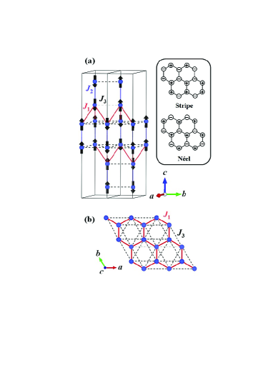
Figure 1: (Color online) (a) Magnetic structure of Ba₂NiTeO₆ PRB93024412 . The blue spheres represent the Ni²⁺ ions. The red solid, blue solid, and black dotted lines represent the pathways of J₁, J₂, and J₃, respectively. VESTA software refforvesta is used for drawing magnetic structure. Inset shows spin arrangement of stripe and $\rm{N\acute{e}el}$ structure. (b) Arrangement of Ni²⁺ ions in buckled honeycomb lattice.

Ba₂NiTeO₆ is a rare experimental realization of the buckled honeycomb lattice antiferromagnet Ba2NiTeO6struc . The magnetic Ni²⁺ ions and the pathways of their interactions J₁, J₂, and J₃ are shown in Fig. 1(a). The two neighboring triangular lattices coupled by the first-neighbor (NN) interaction J₁ form a buckled honeycomb lattice as shown in Fig. 1(b) PRB93024412 . The third-neighbor interaction J₃ corresponds to the next-nearest neighbor (NNN) interaction in the honeycomb lattice. The buckled honeycomb lattices are magnetically coupled by the second-neighbor interaction J₂. Since the J₁ and J₃ have the similar Ni²⁺-O^2--O^2--Ni²⁺ paths owing to the buckled geometry of the honeycomb lattice, they are expected to be comparative and induce strong frustration. The magnetic susceptibility and heat capacity measurements identified a magnetic transition at 8.6 K PRB93024412 . The strong magnetic frustration and/or low dimensionality is indicated from the large frustration parameter ${\theta}_{\rm W}/T_{\rm N}=18.6$, where ${\theta}_{\rm W}$ is Weiss temperature and $T_{\rm N}$ is the magnetic transition temperature. We note that Ba₂CoTeO₆ also includes buckled honeycomb layers DT395490 , and exhibited interesting magnetic phases particularly in the magnetic field PRB93094420 . The material is, however, composed of two subsystems; a buckled honeycomb lattice and a triangular lattice.

Recently, we investigated the magnetic structure of Ba₂NiTeO₆, and we found that the collinear stripe structure with the propagation vector $k_{\bf mag}$ of (0, 0.5, 1) is realized as shown in Fig. 1 PRB93024412 . We classically calculated the phase diagram of $D/J_{1}$ vs $J_{3}/J_{1}$ for the buckled honeycomb lattice antiferromagnet. Here $D$ is the easy-axis type single-ion anisotropy. We demonstrated the existence of the stripe structure that is stabilized by a subtle balance between J₁, J₃, and $D$.

In this paper, we investigate the spin dynamics of the titled compound by using the inelastic neutron scattering technique to identify the spin Hamiltonian. We observed a magnetic excitation having an energy gap at a low temperature. The neutron spectrum is reasonably reproduced by the calculation using linear spin-wave theory. The obtained set of parameters of exchange interaction and single-ion anisotropy are consistent with the location of the stripe structure in the phase diagram of the buckled honeycomb antiferromagnet.

II Experimental Details

The polycrystalline sample was synthesized by the solid state reaction method Onounpublished . Inelastic neutron scattering measurements were performed at the hybrid spectrometer HYSPEC at the Spallation Neutron Source at Oak Ridge National Laboratory HYSPECref . The incident neutron energies $E_{i}$ of 7.5, 15, and 35 meV were independently used. For each of these energies the Fermi chopper frequency was set to be 300 Hz. The full width of the (015) nuclear peak at half maximum along the energy transfer ($\hbar\omega$) direction is evaluated to be 0.25(1), 0.66(3), and 1.95(5) meV for $E_{i}$ = 7.5, 15, and 35 meV, respectively. The low temperatures were achieved by the ORANGE cryostat.

III Results and Analysis

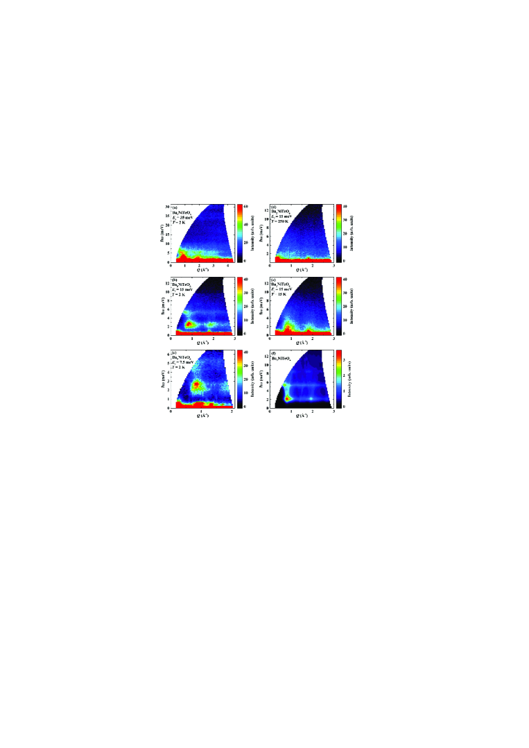
Figure 2: (Color online) INS spectra at 2 K for $E_{i}$ = (a) 35, (b) 15, and (c) 7.5 meV. INS spectra for $E_{i}$ = 15 meV at (d) 250 and (e) 15 K. (f) Calculated spin-wave spectra with $J_{1}$ = 0.8, $J_{2}$ = -0.01, $J_{3}$ = 1.6, $D$ = 1.1 meV.

Figure 2(a), 2(b), and 2(c) show the inelastic neutron scattering (INS) spectra at 2 K for $E_{i}$ = 35, 15, and 7.5 meV, respectively. In Fig. 2(a) excitations having strong intensities are observed at $\hbar\omega\lesssim 10$ meV. They decrease with the increase of $Q$, meaning that the dominant component is magnetic scattering. At $\hbar\omega\sim$ 13, 18, and 25 meV smeared and weak intensities are observed; all of them slightly increase with $Q$, meaning that they are not magnetic excitations. The energy band of the magnetic excitation is, thus, 10 meV. In Figs. 2(b) and 2(c) the structure of the magnetic excitation is clearly observed. It exhibits an energy gap of 2 meV. There are flat features at $\hbar\omega$ = 2.5 and 5.0 meV in the spectrum. In the former two broad maxima are observed at $Q$ = 0.8 and 1.8 Å^-1.

The INS spectrum for $E_{i}$ = 15 meV at 250 K is shown in Fig. 2(d). The excitation observed at 2 K is suppressed, and no clear feature is observed. The smeared excitations are ascribed to paramagnetic spins. Figure 2(e) shows the spectrum at 15 K. Smeared dispersive excitations which indicates a short-range spin correlation are observed. It is consistent with a broad maxima observed in the magnetic susceptibility PRB93024412 .

In order to evaluate the magnetic interactions and the anisotropy from the obtained magnetic excitation, we calculate neutron cross section using spin-wave approximation. Here we consider the Heisenberg model with easy-axis anisotropy as the same as that used in the previous study PRB93024412 , which is given by,

$$H=\sum_{i,j}\textit{J}_{i,j}\mbox{\boldmath$S$}_{i}\cdot\mbox{\boldmath$S$}_{j}-D\sum_{i}S^{2}_{i,z},$$ (1)

where $\mbox{\boldmath$S$}_{i}$ and $S_{i,z}$ represent the vectors for the spin of Ni²⁺ ion at the position of $r_{i}$ and its component along the c axis, respectively. We take the sum in the first term of the Eq. (1) for all the pairing of spins corresponding to J₁, J₂, and J₃ in the unit cells. We assume the stripe structure determined by our previous study PRB93024412 as the ground state. The cross section for this model is calculated by the method described in Ref. 20. We take a powder average in order to compare the calculated spectrum with the experimentally obtained one. The calculated spectrum is convoluted by the Gaussian function. The resolution along $Q$ direction is experimentally obtained from the width of the nuclear (015) peak. The resolution along $\hbar\omega$ direction $d(\hbar\omega)$ is roughly approximated to be $d(\hbar\omega)=0.4789-0.032\hbar\omega$ meV as a function of $\hbar\omega$, which is evaluated from the linear fitting of the instrumental resolution. In order to reproduce the width of the broad peaks in the spectrum, we further convolute the spectrum along the $\hbar\omega$ direction by the Lorentzian function with the width of the Lorentzian function $dL$ of 0.15 meV, which indicates a slight decrease of life time of the excitation. We found that $J_{2}$ is needed to be much smaller than $J_{1}$, $J_{3}$, and $D$ in order to reproduce the flat components in experimentally obtained spectra. $J_{2}$ is negligibly small so that it cannot be evaluated qualitatively. We put negative small value (-0.01 meV) in $J_{2}$ to ensure the stripe structure in the previous study PRB93024412 . The parameters are thus $J_{1}$, $J_{3}$, $D$. We finally determined the parameters to be $J_{1}$ = 0.8 (1), $J_{3}$ = 1.6(1), and $D$ = 1.1(1) meV. The calculated spin-wave spectrum with the parameters $J_{1}$ = 0.8, $J_{3}$ = 1.6, $D$ = 1.1, and $dL$ = 0.15 meV is shown in Fig. 2(f). It reproduces the experimentally obtained spectrum shown in Fig. 2(b).

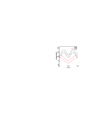
Figure 3: In-plane dispersion for the calculated spin-wave spectra with $J_{1}$ = 0.8, $J_{2}$ = -0.01, $J_{3}$ = 1.6, $D$ = 1.1 meV. Red and black solid lines show the dispersions along the $h$ and $k$ directions in the reciprocal lattice space.

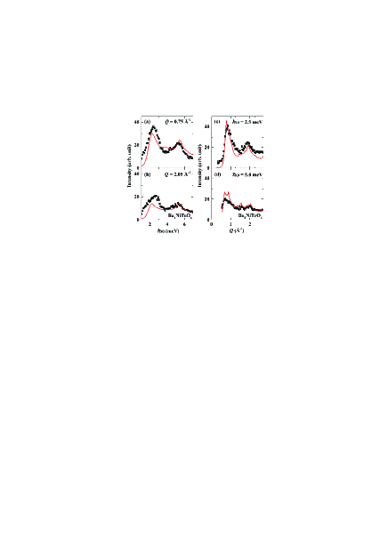
Figure 4: (Color online) (a) One-dimensional cut along energy transfer at $Q$ = 0.75 Å^-1 obtained by integrating intensity with respect to $Q$ from 0.7 to 0.8 Å^-1. (b) One-dimensional cut along energy transfer at $Q$ = 2.05 Å^-1 obtained by integrating intensity with respect to $Q$ from 2.0 to 2.1 Å^-1. (c) One-dimensional cut along $Q$ at $\hbar\omega$ = 2.5 meV obtained by integrating intensity with respect to $\hbar\omega$ from 2.3 to 2.7 meV. (d) One-dimensional cut along $Q$ at $\hbar\omega$ = 5.0 meV obtained by integrating intensity with respect to $\hbar\omega$ from 4.8 to 5.2 meV. Square symbols represent the experimental data while the curves depict the calculated values. Incoherent elastic component is subtracted from the the experimental data. The detail is shown in the main text.

Here we discuss the detail of the calculated spectrum. We show the in-plane dispersions in Fig. 3. The difference of the period for the dispersions between the $h$ and $k$ directions corresponds to the modulation of the stripe order. The bottom of the dispersion along the $h$ direction is located at 2.2 and 5.4 meV.

Let us compare the one-dimensional cuts of the spectra shown in Fig. 2(b) and 2(f) in order to compare them more in detail. In order to exclude the incoherent elastic component from the experimental data, we evaluate it by fitting the peak at $\hbar\omega$ = 0 meV in the one-dimensional cut along energy transfer obtained by integrating intensity with respect to $Q$ from 0.7 to 0.8 by using Gaussian function, and subtracted it from the one-dimensional cuts shown in Fig. 4(a), 4(b), 4(c), and 4(d). Figure 4(a) and 4(b) show the one-dimensional cuts along energy transfer at $Q$ = 0.75 and 2.05 Å^-1 obtained by integrating intensity with respect to $Q$ from 0.7 to 0.8 and from 2.0 to 2.1 Å^-1, respectively. One-dimensional cuts along $Q$ at $\hbar\omega$ = 2.5 and 5.0 meV are shown in Fig. 4(c) and 4(d), which are obtained by integrating intensity with respect to $\hbar\omega$ from 2.3 to 2.7 and from 4.8 to 5.2 meV, respectively. We clearly see that the calculation roughly reproduces the broad peaks along $Q$ direction observed at $\hbar\omega$ = 2.5 meV and those along $\hbar\omega$ direction at $Q$ = 0.75 Å^-1. More precise estimate of the magnetic interactions and anisotropy is needed for better reproduction, which can be achieved by the single-crystal neutron scattering study.

IV Discussion

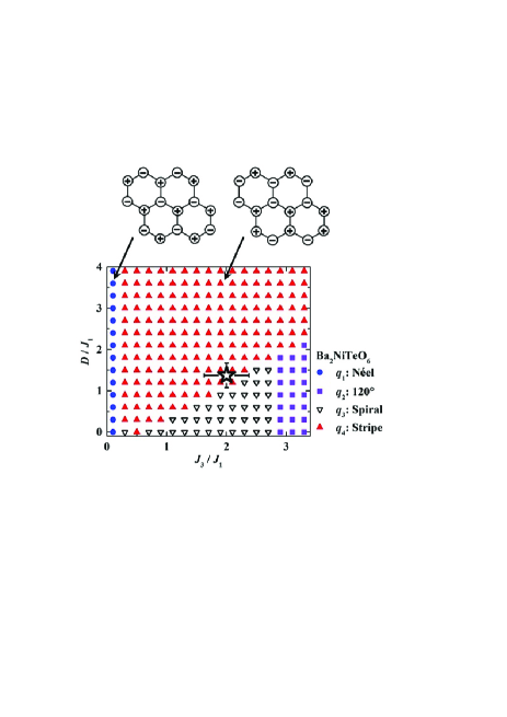
Figure 5: Magnetic phase diagram for classical ground state. The $\mbox{\boldmath$q$}_{1}$ and $\mbox{\boldmath$q$}_{4}$ phases are sketched above the diagram. The $\mbox{\boldmath$q$}_{4}$ phase corresponds to the experimentally determined magnetic structure. The details of the $\mbox{\boldmath$q$}_{1}$, $\mbox{\boldmath$q$}_{2}$, $\mbox{\boldmath$q$}_{3}$, and $\mbox{\boldmath$q$}_{4}$ phases are described in Ref. 13.

We first discuss the evaluated parameters of magnetic interactions and anisotropy in the phase diagram in the previous study PRB93024412 . Figure 5 shows the classical phase diagram in the range of $0<J_{3}/J_{1}<3.2$ and $0<D/J_{1}<4$. Néel, 120 degree, and spiral structures are realized in the $\mbox{\boldmath$q$}_{1}$, $\mbox{\boldmath$q$}_{2}$, $\mbox{\boldmath$q$}_{3}$ phases, respectively. In the $\mbox{\boldmath$q$}_{4}$ phase, the stripe structure is stabilized. We note that the $\mbox{\boldmath$q$}_{4}$ phase is only stable at $J_{3}/J_{1}=0.5$ in the case of $D=0$ EPJB20241 . The $J_{3}$ induces geometrical frustration and supports spiral structure. The easy-axis anisotropy, on the other hand, suppresses the spiral structure and stabilizes the stripe structure. This means that the stripe structure appears as the result of competition between geometrical frustration in the buckled honeycomb lattice and the easy-axis anisotropy. The open star symbol in the phase diagram represents the parameters obtained in the present experiment. The symbol is located in the region of stripe structure, meaning that the obtained parameters from the INS experiment are consistent with the classical phase diagram of the ground state.

Next, let us discuss the magnetic behavior above $T_{\rm N}$ of this compound. The small $J_{2}$ suggests that the buckled honeycomb lattices in Ba₂NiTeO₆ are magnetically isolated. The strong magnetic frustration is expected from the comparative magnetic interactions $J_{1}$ and $J_{3}$. These obtained results are consistent with the broad maximum of the magnetic susceptibility and heat capacity indicating the short-range magnetic correlation of Ni²⁺ ions PRB93024412 . The magnetic susceptibility of the powder sample follows the Curie-Weiss law above 100 K. We expects that the Weiss temperature depends on the magnetic interactions and anisotropy, and it is a good indicator for examining whether the evaluated parameters are quantitatively consistent with the magnetic properties. Then, let us derive the Weiss temperature analytically by the mean-field approximation. We safely neglect the $J_{2}$ in the calculation because of its small value. We consider the Heisenberg Hamiltonian with the easy-axis anisotropy and applied magnetic field $H$, which is given by,

$$\mathcal{H}=\sum_{i,j}\textit{J}_{i,j}\mbox{\boldmath$S$}_{i}\cdot\mbox{\boldmath$S$}_{j}-D\sum_{i}S^{2}_{i,z}+\sum_{i}g\mu_{\rm B}\mbox{\boldmath$S$}_{i}\cdot\mbox{\boldmath$H$}.$$ (2)

By using the mean-field approximation, the Hamiltonian is rewritten as

$$\mathcal{H}=-\sum_{i}DS^{2}_{i,z}+\sum_{i}g\mu_{\rm B}\mbox{\boldmath$S$}_{i}\cdot\mbox{\boldmath$H$}^{\prime},$$ (3)

where $\mbox{\boldmath$H$}^{\prime}$ is the sum of the molecular and applied magnetic field, which is given by

$$\mbox{\boldmath$H$}^{\prime}=\mbox{\boldmath$H$}+\frac{\sum_{j}\textit{J}_{i,j}<\mbox{\boldmath$S$}_{j}>}{g\mu_{\rm B}}=\mbox{\boldmath$H$}+\frac{(3J_{1}+6J_{3})<\mbox{\boldmath$S$}_{i}>}{g\mu_{\rm B}}.$$ (4)

For simplicity, we assume that the applied magnetic field is parallel to the crystallographic $c$ axis, which is the magnetic easy axis. Then, the Hamiltonian is modified as

$$\mathcal{H}=-\sum_{i}DS^{2}_{i,z}+\sum_{i}g\mu_{\rm B}S_{i,z}H^{\prime}.$$ (5)

In mean-field approximation the eigenenergy of the spin is independent of the position $r_{i}$, and the energy is given by

$$\epsilon_{m}=-Dm^{2}+g\mu_{\rm B}mH^{\prime},$$ (6)

where $m$ is the magnetic quantum number ($m$ = 1, 0, -1). Then, we can evaluate $<S_{z}>$ by using the partition function expressed as,

$$<S_{z}>=\cfrac{\sum_{m}m\exp(\cfrac{-\epsilon_{m}}{k_{\rm B}T})}{\sum_{m}\exp(\cfrac{-\epsilon_{m}}{k_{\rm B}T})},$$ (7)

In the case of $k_{\rm B}T>>\mid\epsilon_{m}\mid$, we can approximate the exponential functions by the linear functions. We substitute the equations (4) and (6) for the equation (7), and derive $<S_{z}>$ as

$$<S_{z}>=\cfrac{-2g\mu_{\rm B}H}{3k_{\rm B}T+2(3J_{1}+6J_{3}+D)}.$$ (8)

Then, we obtained the magnetic susceptibility following the Curie-Weiss law, which is given by

$$\chi=\cfrac{-g\mu_{\rm B}<S_{z}>}{H}=\cfrac{C}{T+\theta},$$ (9)

where $C$ is the Curie constant. We finally derive the Weiss temperature $\theta$ as

$$\theta=\cfrac{2(3J_{1}+6J_{3}+D)}{3k_{\rm B}}.$$ (10)

Substitute the parameters estimated from the INS experiment, $J_{1}$ = 0.8, $J_{3}$ = 1.6, $D$ = 1.1 meV, for the equation (10), and we obtained $\theta$ $\sim$ 101 K. It is consistent with the experimentally obtained value of 128(2) K from the magnetic susceptibility for the single crystal sample in the case that $H$ is parallel to the $c$ axis Onounpublished . Thus, the consistency among the independent experiments, the INS and bulk properties measurements, is confirmed.

Here we discuss the difference of the energy scale between the magnetic interactions $J_{1}$ and $J_{3}$. The superexchange interactions via the Ni²⁺-O^2--O^2--Ni²⁺ pathways for $J_{1}$ and $J_{3}$ are expected to be antiferromagnetic from the Goodenough-Kanamori rule KanamoriGoodenoughRef . Additionally, the antiferromagnetic contribution from the Ni²⁺-O^2--Te⁶⁺-O^2--Ni²⁺ pathways are also expected as discussed for Sr₂CuTeO₆ PRB93054426 . On the other hand, these Te⁶⁺-mediated interactions favors $J_{1}>J_{3}$ because there are two pathways for $J_{1}$ in contrast to a single pathway for $J_{3}$, which is not consistent with the obtained results. We expects that the result $J_{1}<J_{3}$ is due to the distortion of NiO₆ octahedra which change the Ni²⁺-O^2--O^2--Ni²⁺ bond angle. Theoretical calculation of the magnetic interactions is needed for further investigation.

Finally we compare the magnetic property of honeycomb lattice for Ba₂NiTeO₆ with that for other honeycomb lattice antiferromagnets. In Ba₂CoTeO₆ where the buckled honeycomb and triangular layers are alternately stacked, the magnetic order in the honeycomb layer is similar to that of Ba₂NiTeO₆ DT395490 . The ratio of the NNN interaction to the NN interaction in Ba₂CoTeO₆ is estimated to be about $1/4$ of that in Ba₂NiTeO₆ PRB93094420 . This means that the magnetic interactions are much modified by the substitution of Ni²⁺ ions for Co²⁺ ions, and nevertheless, the stripe order is retained. The result is consistent with our phase diagram in Fig. 5; the stripe order is robust to $J_{3}/J_{1}$ under the existence of the the easy-axis type anisotropy, and particularly at $J_{3}/J_{1}$ = 0.5 solely the stripe order does exist regardless of the magnitude of $D$.

In contrast with the buckled honycomb lattice magnets, the thrid-neighbor interaction is rather enhanced in the regular honeycomb lattice magnets formed by edge-shared octahedra of the ligands such as BaNi₂P₂O₈ JMMM151021 and BaCo₂As₂O₈ PhysicaBC86660 . The magnetic frustration induced by the competition between the NN and third-neighbor interactions leads to various states, which had been studied in the accumulative studies PRB65144443 ; JMMM151021 ; PhysicaBC86660 ; PRL105187201 ; PRB94214416 ; Regnault89 . Meanwhile the magnetic states of the buckled honeycomb lattice antiferromagnets has been less explored because of a small amount of the model compounds. The investigation on other model compounds are needed for further study.

V Summary

We carried out the INS experiment for the buckled honeycomb lattice antiferromagnet Ba₂NiTeO₆ in order to investigate the magnetic interaction and anisotropy quantitatively. The magnetic excitation with the band energy of 10 meV and an energy gap of 2 meV is observed at 2 K. We perform the spin-wave calculation and evaluate the magnetic interaction and anisotropy. The spectrum at 2 K is well reproduced by the calculated one with the parameters $J_{1}$ = 0.8(1), $J_{3}$ = 1.6(1), $D$ = 1.1(1) meV, $J_{2}$ is negligibly small. The evaluated parameters are located in the range of stripe phase in the phase diagram of the frustrated honeycomb antiferromagnet. They are consistent with the Weiss temperature independently estimated from the bulk magnetic property measurement. The consistency among the INS experiment, magnetic susceptibility measurement, and the calculation of the ground state reveals that Ba₂NiTeO₆ is an experimental realization of the two-dimensional honeycomb lattice antiferromanget and that the stripe structure is the result of the competition between the geometrical frustration of the lattice and the easy-axis anisotropy of Ni spins.

- (1) E. Rastelli, A. Tassi, and L. Reatto, Physica B & C 97, 1 (1979).
- (2) J. B. Fouet, P. Sindzingre, and C. Lhuillier, Eur. Phys. J. B 20, 241 (2001).
- (3) H. Mosadeq, F. Shahbazi, and S. A. Jafari, J. Phys.: Condens. Matter 23, 226006 (2011).
- (4) A. F. Albuquerque, D. Schwandt, B. Hetényi, S. Capponi, M. Mambrini, and A. M. Läuchli, Phys. Rev. B 84, 024406 (2011).
- (5) A. Kitaev, Ann. Phys. 321, 2 (2006).
- (6) G. Jackeli and G. Khaliullin, Phys. Rev. Lett. 102, 017205 (2009).
- (7) N. Rogado, Q. Huang, J. W. Lynn, A. P. Ramirez, D. Huse, and R. J. Cava, Phys. Rev. B 65, 144443 (2002).
- (8) L. P. Regnault, J. Y. Henry, J. Rossat-Mignod, and A. D. Combarieu, J. Mag. Mag. Mater. 15-18, 1021 (1980).
- (9) L. P. Regnault, P. Burlet, and J. Rossat-Mignod, Physica B+C 86-88, 660 (1977).
- (10) M. Matsuda, M. Azuma, M. Tokunaga, Y. Shimakawa, and N. Kumada, Phys. Rev. Lett. 105, 187201 (2010).
- (11) E. Lefrançois, M. Songvilay, J. Robert, G. Nataf, E. Jordan, L. Chaix, C. V. Colin, P. Lejay, A. Hadj-Azzem, R. Ballou, and V. Simonet, Phys. Rev. B 94, 214416 (2016).
- (12) J. A. Sears, M. Songvilay, K. W. Plumb, J. P. Clancy, Y. Qiu, Y. Zhao, D. Parshall, and Y.-J. Kim, Phys. Rev. B 91, 144420 (2015).
- (13) S. Asai, M. Soda, K. Kasatani, T. Ono, M. Avdeev, and T. Masuda, Phys. Rev. B 93, 024412 (2016).
- (14) P. Köhl, U. Müller, and D. Reinen, Z. Anorg. Allg. Chem. 392, 124 (1972).
- (15) K. Momma and F. Izumi, J. Appl. Crystallogr. 44, 1272 (2011).
- (16) S. A. Ivanov, P. Nordblad, R. Mathieu, R. Tellgren, and C. Ritter, Dalton Trans. 39, 5490 (2010).
- (17) P. Chanlert, N. Kurita, H. Tanaka, D. Goto, A. Matsuo, and K. Kindo, Phys. Rev. B 93, 094420 (2016).
- (18) T. Ono et al., (private communication).
- (19) B. Winn, U. Filges, V. O. Garlea, M. Graves-Brook, M. Hagen, C. Jiang, M. Kenzelmann, L. Passell, S. M. Shapiro, X. Tong, and I. Zaliznyak, EJP Web Conf. 83, 03017 (2015).
- (20) A. W. Sáenz, Phys. Rev. 125, 1940 (1962).
- (21) J. Kanamori, J. Phys. Chem. Solid 10, 87 (1959).
- (22) T. Koga, N. Kurita, M. Avdeev, S. Danilkin, T. J. Sato, and H. Tanaka, Phys. Rev. B 93, 054426 (2016).
- (23) L. P. Regnault, C. Lartigue, J. F. Legrand, B. Farago, J. Rossat-Mignod, and J. Y. Henry, Physica B 156-157, 298 (1989).