Secondary Fans and Secondary Polyhedra
of Punctured Riemann Surfaces
Abstract.
A famous construction of Gel’fand, Kapranov and Zelevinsky associates to each finite point configuration a polyhedral fan, which stratifies the space of weight vectors by the combinatorial types of regular subdivisions of . That fan arises as the normal fan of a convex polytope. In a completely analogous way we associate to each hyperbolic Riemann surface with punctures a polyhedral fan. Its cones correspond to the ideal cell decompositions of that occur as the horocyclic Delaunay decompositions which arise via the convex hull construction of Epstein and Penner. Similar to the classical case, this secondary fan of turns out to be the normal fan of a convex polyhedron, the secondary polyhedron of .
Key words and phrases:
ideal triangulations; decorated Teichmüller space2010 Mathematics Subject Classification:
30F60 (32G15, 52B12, 57M50)1. Introduction
Our goal is to employ techniques from geometric combinatorics to further the understanding of the space of ideal Delaunay decompositions of a punctured Riemann surface. We believe that this is relevant to researchers in hyperbolic geometry. Combinatorialists may benefit from seeing how far their methods carry.
A punctured Riemann surface (of genus with punctures) is , the closed oriented surface of genus with punctures, equipped with a complete hyperbolic metric of finite area. Throughout this article we assume that the Euler characteristic is negative and . The punctures of correspond to cusps of (see Figure 5). The space of complete hyperbolic metrics with finite area on , up to isotopy, is known as the Teichmüller space . Penner [Pen87] suggested to equip a punctured Riemann surface with an additional choice of horocycles, one for each puncture. This is known as a decoration of . Via their lengths, such a choice of horocycles can be described by a vector of positive real numbers, the weight vector of the decoration. In this way we obtain the decorated Teichmüller space , which is a trivial -bundle over . Akiyoshi [Aki01] used partial decorations with weight vectors in .
Epstein and Penner [EP88, Pen87] employed a convex hull construction to show that a decoration of determines an ideal cell decomposition of . This construction involves the hyperboloid model of the hyperbolic plane and the representation of as a quotient with respect to a group of hyperbolic isometries. Distinguishing decorated Riemann surfaces by the induced decomposition of , one obtains a cell decomposition of the decorated Teichmüller space [Pen87, Pen12]. In this article we focus on individual fibers of , i.e., we consider fixed Riemann surfaces with variable decoration. If the Riemann surface is fixed, only a finite number of ideal cell decompositions occur as result of the the convex hull construction [Aki01].
Our first observation is that for a fixed Riemann surface , the weight vectors which induce the same ideal cell decomposition of form a relatively open polyhedral cone (Theorem 5.5). Moreover, since these secondary cones meet face-to-face, we obtain a polyhedral fan, the secondary fan of (cf. Definition 5.7). In particular, this shows that the refinement poset of ideal Delaunay decompositions is a lattice with the minimal and maximal elements removed: If the set of ideal Delaunay decompositions contains a common refinement for two of its elements, then it contains a unique coarsest common refinement, and if it contains a common coarsening, then it contains a unique finest common coarsening.
This is very similar to the secondary cones and secondary fans of point configurations in , which were introduced by Gel’fand, Kapranov and Zelevinsky [GKZ08], and which are the fundamental building blocks of a theory with numerous applications to combinatorics, optimization, algebra and other parts of mathematics; see the monograph of De Loera, Rambau and Santos [DLRS10]. A key theorem says that the secondary fan of a Euclidean point configuration arises as the normal fan of a convex polytope, the secondary polytope of the point configuration. Our main result (Theorem 6.6) is a complete analog for punctured Riemann surfaces: The secondary fan of is the normal fan of a secondary polyhedron of (cf. Definition 6.5).
Despite the close analogy, there are some notable differences between the classical theory of secondary polytopes and our version for punctured Riemann surfaces. First of all, for punctured Riemann surfaces only non-negative weights are allowed because they are the lengths of the horocycles at the punctures. This prevents our secondary polyhedra from being bounded. While all vertices of a secondary polytope of a point configuration correspond to triangulations, the vertices of a secondary polyhedron of a punctured Riemann surface correspond to coarsest Delaunay decompositions, which are not necessarily ideal triangulations. Moreover, while a point configuration in determines a unique secondary polytope, our construction associates a unique secondary polyhedron to each pair consisting of a punctured Riemann surface and a point (cf. Section 6). Thus, our construction yields a polyhedron bundle over the Riemann surface . This is reminiscent of the notion of fiber polytopes [BS92], but here the base space is a punctured Riemann surface instead of a polytope.
This research was originally motivated by a recent variational method to construct ideal hyperbolic polyhedra with prescribed intrinsic metric, or equivalently, to compute discrete uniformizations of piecewise Euclidean surfaces [Spr17]. The complexity of this method depends on the complexity of the flip algorithm for the Epstein–Penner convex hull construction [Wee93, TW16]. We expect that the correspondence between ideal Delaunay decompositions of a punctured Riemann surface and faces of a secondary polyhedron will shed further light on that method.
The paper is organized in a way to make it accessible for audiences from both geometry and combinatorics. To describe the full setup thus requires an unusually long preparation. Experts in both fields might want to start with the new results in Section 5 right away. Frequent references to the introductory sections are meant as an aid for picking up our notation. In Section 2 we begin with reviewing the classical GKZ construction of secondary polytopes of point configurations in . This will subsequently allow to point out the similarities and the differences between the classical theory and our version for punctured Riemann surfaces. In Section 3 we recall basic facts from hyperbolic geometry. This is mainly to introduce our notation, but also for describing explicitly how to translate between various models of the hyperbolic plane. This is important as the proofs of our main results require to switch freely between several models. After a brief review of punctured Riemann surfaces and Penner’s coordinates on decorated Teichmüller spaces in Section 4, we finally define the secondary fan of a punctured Riemann surface in Section 5. Ideal cell decompositions of a Riemann surface with punctures correspond to secondary cones in , which form the secondary fan. The construction of secondary polyhedra and our main result, Theorem 6.6, are the topic of Section 6. Sections 5 and 6 are illustrated with many explicit examples. The latter have been obtained via an implementation in polymake [GJ00], and the method is briefly explained in Section 7. We close the paper with remarks on possible generalizations and open questions in Section 8.
For helpful discussions we are indebted to Stephan Tillmann.
2. The classical GKZ construction
In this section, we quickly recall the classical constructions of secondary fans and secondary polytopes for point configurations in . The ideas were developed by Gel’fand, Kapranov and Zelevinsky [GKZ08]; see also [DLRS10, Chap. 5]. In Sections 5 and 6 we will describe analogous constructions for punctured Riemann surfaces instead of point configurations in .
Let be a non-empty finite subset with elements and let be its convex hull. For simplicity we assume that is not contained in a proper affine subspace of , so that is a -dimensional polytope and in particular . A polytopal subdivision of is a polytopal complex whose carrier is and whose vertex set is a subset of . Note that it is not required that all points in are vertices of . Only the vertices of necessarily occur as vertices of . A triangulation of is a polytopal subdivision of whose elements are simplices.
For any assignment of real numbers to elements of , let be the function
| (1) |
where the minimum is taken over all affine functions
| (2) |
satisfying
| (3) |
The function is a piecewise linear concave function. Its graph
is the upper boundary of the convex hull of the point set in .
Let be the polytopal subdivision of that contains a polytope if and only if there is an affine function (2) satisfying (3) such that
Vertical projection maps the faces of bijectively onto the cells of . A polytopal subdivision of is called regular if for some . The secondary cone of a polytopal subdivision of is defined by
| (4) |
where we write if refines , i.e., if every cell of is contained in a some cell of . The secondary cones are indeed polyhedral cones. To see this, we use the functions defined below to derive linear equations and inequalities describing the secondary cones. We will also use the functions to define the secondary polytopes.
For any triangulation of and any , let
| (5) |
be the linear interpolation of with respect to , i.e., the unique piecewise linear function that is affine on each simplex of and satisfies
Then if and only if is concave, so
| (6) |
On each -simplex , the function coincides with the affine function
| (7) |
where denotes the oriented volume of an oriented -simplex in , i.e.,
The function is concave if and only if for every pair
of -simplices sharing a -face we have
| (8) |
If the simplex is positively oriented, i.e., , then inequality (8) is equivalent to
| (9) |
So if and only if satisfies the inequalities (9) for all pairs of -simplices sharing a -face. More generally, one obtains the following characterization for arbitrary subdivisions:
Lemma 2.1.
Let be a polytopal subdivision of and let be a triangulation of refining . Then the following statements for are equivalent:
-
(i)
-
(ii)
For any two -simplices sharing a -face, where is positively oriented, satisfies inequality (9), and equality holds if both -simplices of are contained in the same -cell of .
In particular, Lemma 2.1 implies that the secondary cones are closed polyhedral cones. The following lemma is also not difficult to see:
Lemma 2.2.
A secondary cone has non-empty interior in if and only if the polytopal subdivision of is in fact a regular triangulation with vertex set equal to .
We finally arrive at the first fundamental result of the classical GKZ-theory:
Theorem and Definition 2.3 (secondary fan).
The collection of secondary cones of regular subdivisions,
| (10) |
is a polyhedral fan with support , called the secondary fan of the point configuration . More specifically, the following holds for all and all regular subdivisions and of :
-
(i)
Every is contained in .
-
(ii)
if and only if is a face of . In particular, implies .
-
(iii)
There is a uniquely determined finest common coarsening of and among all regular subdivisions, and .
Moreover,
-
(iv)
the top-dimensional cones in the secondary fan are precisely the secondary cones of regular triangulations with vertex set .
Remark 2.4.
The analogous statements to Lemma 2.2 and hence Theorem 2.3 (iv) do not hold in the setting of punctured Riemann surfaces (cf. Section 5). A top-dimensional cone in the secondary fan of a punctured Riemann surface may correspond to a Delaunay decomposition that is not an ideal triangulation. In other words, not all finest Delaunay decompositions are ideal triangulations.
For every triangulation of let the function be defined by
| (11) |
where all simplices are positively oriented. Since is a linear function for every triangulation , we can interpet as the function
where is the set of triangulations of and is the dual vector space of . The coordinate vector of with respect to the canonical basis of ,
| (12) |
is called the GKZ-vector of the triangulation and often identified with a vector in via a numbering of the elements of .
Definition 2.5.
(secondary polytope) The secondary polytope is the convex hull of the linear functionals , i.e.,
| (13) |
For a (bounded or unbounded) polytope in a finite dimensional real vector space , and a face of , the normal cone is the cone of all functionals in the dual vector space that attain their maximal value in at all points of . The dimensions are complementary:
The normal fan of is the fan containing the normal cones of all faces . Note that the normal fan is complete, i.e., , if and only if the polytope is bounded.
The following theorem is the second fundamental result of the classical GKZ-theory.
Theorem 2.6.
The normal fan of the secondary polytope is the secondary fan .
This follows directly from the definitions and the fact that a triangulation maximizes the integral in (11) if and only if is concave.
It should be mentioned that the dimension of the secondary polytope of is strictly less than , corresponding to the fact that all cones of the secondary fan contain a nontrivial subspace of . Indeed, if is the restriction of an affine function (2) to , then , and therefore is the face lattice of itself, and for every subdivision of . Thus, all secondary cones contain the -dimensional linear subspace
| (14) |
Also, if then for any triangulation , , where is the barycenter of . Therefore the secondary polytope is contained in an affine subspace of that is spanned by the -dimensional annihilator . In contrast, our secondary polyhedra of punctured Riemann surfaces will turn out to be full-dimensional.
3. The Hyperbolic Plane
We continue with a brief discussion of hyperbolic geometry in order to introduce our notation and terminology. For further reading we suggest [CFKP97], [Thu97] or [Kat92]. Minkowski -space, denoted as , is the three-dimensional real vector space together with the indefinite scalar product
The set of points in with is the standard hyperboloid of two sheets. Its upper sheet
is equipped with the Riemannian metric induced by restricting the Minkowski scalar product to tangent hyperplanes. This gives rise to the hyperboloid model of the hyperbolic plane. Its points are the points in , and geodesics (or [hyperbolic] lines) are the intersections of with planes through the origin. The group of linear transformations with determinant that preserve the Minkowski scalar product and map the upper sheet of the hyperboloid to itself acts on the hyperbolic plane as the group of orientation preserving isometries.
A ray in the positive light cone
is called an ideal point of . The set of ideal points is called the ideal boundary of . Two distinct ideal points span a hyperplane through the origin. The intersection of that hyperplane with yields the geodesic connecting the two ideal points. Furthermore, each point defines the horocycle
centered at the ideal point . Horocycles are limiting cases of circles in the hyperbolic plane as their radii tend to infinity and their centers tend to an ideal point.
Other models of the hyperbolic plane arise via projections. These include the ones below, all of which are rotationally symmetric with respect to the vertical axis; see Figure 1 for a sketch. In each case the hyperbolic metric is carried over by the respective projection.
-
(i)
The Beltrami–Klein model (or projective model) is obtained by projecting from the origin onto the open unit disk at height . The ideal boundary is projected to the topological boundary of this disk. Geodesics are Euclidean line segments within .
-
(ii)
The hemisphere model is obtained from by stereographically projecting through the point onto the northern hemisphere of the unit sphere. Its equator forms the ideal boundary and geodesics are intersections of the hemisphere with hyperplanes orthogonal to the -plane.
Projection along vertical lines maps directly from the Beltrami–Klein model to the hemisphere model and vice versa. That is, a point in the Beltrami–Klein model corresponds to the point in the hemisphere model.
-
(iii)
The half-plane model is obtained from by stereographic projection through the point onto the upper half-plane , which is identified with the upper half-plane of the complex plane . In this model, the ideal boundary is , geodesics are half circles orthogonal to the real axis or Euclidean vertical lines, and horocycles appear as Euclidean circles tangent to the real line or as horizontal lines. The group of orientation preserving isometries becomes the group of fractional linear transformations.
While we mostly work with the hyperboloid and half-plane model, the hemisphere model and its “light cylinder” (16) play an important role in the construction of secondary polyhedra in Section 6. The stereographic projection mapping the hyperboloid to the hemisphere (cf. Figure 1) is the restriction of a projective transformation to . In affine coordinates it is given by
| (15) |
From the standpoint of projective geometry, the hyperboloid model and the hemisphere model are therefore just different affine views of the same projective model. The transformation (15) maps the positive light cone to the cylinder
| (16) |
Points in represent horocycles in the hemisphere model. Explicitly, corresponds to the horocycle
Consider two horocycles centered at two distinct ideal points. The signed hyperbolic distance between and is measured along the geodesic connecting their centers, and the sign is taken negative if and only if the horocycles intersect, see Figure 2. Following Penner [Pen12, Chapter 1, §4.1], we define the -length of to be
If the two horocycles are given as and for two light cone vectors , the former definition yields
| (17) |
An ideal triangle is the closed region in the hyperbolic plane that is bounded by three geodesics (the sides) connecting three ideal points (the vertices). A decoration of an ideal triangle is a triple of horocycles centered at the vertices. Such a decoration gives rise to three -lengths and , one along each edge, see Figure 3. The hyperbolic length of the horocyclic arc within the triangle at a vertex is called the -length at the vertex. In the “trigonometry” of decorated ideal triangles, -lengths and -lengths play a role similar to the side lengths and angles of ordinary trigonometry.
Later we will consider ideal triangulations of punctured Riemann surfaces, and then some of the vertices of a triangle may correspond to the same ideal point of the surface. For this reason, we will need more sophisticated notation than just labelling the -lengths by an incident triangle-vertex pair. The standard orientation of the hyperbolic plane induces a cyclic order of the sides of a triangle. If the sides are in this cyclic order, we label the three -lengths of by and , see Figure 3. The - and the -lengths of a decorated ideal triangle are related via
| (18) |
see [Pen12, Chapter 1, §4.2].
Ideal triangles generalize to arbitrary ideal polygons, with or without decorations. An ideal quadrilateral admits exactly two triangulations. If the edges are cyclically ordered, then each triangulation is determined by the choice of either the diagonal , yielding the two triangles and , or the diagonal , yielding the triangles and , see Figure 4. Substituting one diagonal by the other is referred to as a diagonal flip. A decoration with horocycles at the four vertices gives rise to six -lengths. They satisfy the Ptolomy relation
| (19) |
which follows immediately from (18), see Figure 4 and [Pen12, Chapter 1, §4.3].
4. Punctured Riemann Surfaces
A Riemann surface is a complex one-dimensional manifold. Here we are only interested in punctured Riemann surfaces, i.e., compact Riemann surfaces with a finite number of points removed. Morevover, we consider only punctured Riemann surfaces with negative Euler characteristic, which excludes only spheres with one or two punctures. Under this assumption, a punctured Riemann surface admits a conformal complete hyperbolic metric with finite area, which is unique up isotopy. The punctures of the Riemann surface correspond to cusps of the hyperbolic surface (cf. Figure 5). Henceforth, we take the metric point of view and consider punctured Riemann surfaces as complete hyperbolic surfaces with finite area and at least one cusp.
Riemann surfaces arise in many concrete forms, and this accounts for the enormous richness of the theory. In this section we briefly review two of these forms: quotients of the hyperbolic plane by groups of isometries, and surfaces constructed by gluing decorated ideal triangles together. These two points of view are particularly useful for the definition of the secondary fan (cf. Section 5) and the construction of secondary polyhedra (cf. Section 6). For a more detailed discussion see, e.g., [Bea95, Kap09, Kat92, Leh66, Pen87, Pen12]. Instead of the half-plane model with isometry group , which is the more classical approach, we use the hyperboloid model with isometry group because this is how the Epstein–Penner convex hull construction is usually described (cf. Section 5).
The group of orientation-preserving isometries of the hyperbolic plane acts naturally on the ideal boundary . An isometry is elliptic, parabolic or hyperbolic if the number of fixed ideal points is or , respectively. Only the identity fixes more than two ideal points. An elliptic isometry has exactly one fixed point in . A Fuchsian group is a discrete subgroup of . It is a fundamental result that a subgroup of is discrete if and only if it acts properly discontinuously on . Furthermore, acts freely if and only if it does not contain any elliptic elements. In this case, the quotient
| (20) |
with the induced hyperbolic metric is the Riemann surface defined by . Since is simply connected, is canonically isomorphic to the fundamental group of and acts by deck transformations. The quotient with repspect to another Fuchsian group is isometric to if and only if and are conjugate subgroups of .
In general, the area of the quotient is not finite. If it is finite, then the group is called a Fuchsian group of the first kind. In particular, this entails that is finitely generated. Suppose further that contains a parabolic element with as its unique ideal fixed point. Then the -orbit of correponds to a cusp of , see Figure 5. From now on we suppose that the surface has finite area and at least one cusp.
We will now discuss how the notions of horocycles, -lengths and -lengths (cf. Section 3) carry over to decorated Riemann surfaces and ideal triangulations. This will lead to the second point of view, surfaces glued from ideal triangles, and to some practical formulas, which we will use in Sections 5 and 6.
A horocycle at a cusp of is a -orbit of horocycles centered at the parabolic fixed points of the corresponding -orbit. If such a horocycle in is sufficiently small then its image under the projection to is an embedded closed curve around the cusp. A decoration of is a choice of one horocycle at each cusp.
An ideal cell decomposition of is a family of ideal polygons such that (i) the polygons cover and (ii) any two polygons intersect in a common edge, or the intersection is empty. If each ideal polygon is an ideal triangle, the ideal cell decomposition is called an ideal triangulation.
An ideal cell decomposition of is a -invariant ideal cell decomposition of , all vertices of which are parabolic fixed points of . It decomposes into finitely many ideal polygons, the faces of , which are glued along their sides, the edges of . If all faces are triangles, is an ideal triangulation of .
Now let be a punctured Riemann surface, decorated with a horocycle at each cusp, and let be an ideal triangulation of . The -length of an edge of is defined by (17), where , are the horocycles at the ends of a lift of to the universal cover .
Conversely, if is an ideal triangulation of the topological surface of genus with punctures, a positive function on the set of edges determines a complete hyperbolic metric with finite area on , uniquely up to isotopy, together with decorating horocycles at the cusps. Simply construct decorated ideal triangles with -lengths determined by , one triangle for each face of , and glue them together according to the combinatorics of so that the horocycles fit toghether at the vertices.
The -lengths of horocyclic arcs in the corners of the triangles of are determined by the -lengths of the edges via equation (18). If is a triangle of with edges , , in the cyclic order induced by the orientation of , we label the corners of by , , , and denote the corresponding -lengths by , , .
Remark 4.1.
This notation is valid even if two sides of the triangle are glued together and correspond to the same edge of the triangulation . For instance, if the edges of are in cyclic order, then the three corners are labelled , and .
The total length of the decorating horocycle at the cusp is
| (21) |
where the sum is taken over all corners of incident with cusp . We call the weight of cusp of the decorated surface. Note that the weight of a cusp does not depend on the ideal triangulation.
5. The Secondary Fan
Epstein and Penner’s convex hull construction [EP88, Pen87, Pen12] is fundamental for the definition of the secondary fan of a punctured Riemann surface (cf. 5.7). This construction produces an ideal cell decomposition for each decorated Riemann surface with cusps in the following way. By definition, the horocycle at the th cusp corresponds to a -orbit of points in the positive light cone . Their union is a countably infinite set as is finitely generated. Now consider the Euclidean convex hull
| (22) |
The following is a key observation.
Proposition 5.1 ([EP88], [Pen12, Chapter 4, §1]).
The union of -orbits corresponding to a decoration of is discrete and closed in . The faces of the boundary of the convex hull project to an ideal cell decomposition of .
Akiyoshi [Aki01] generalized the convex hull construction for partially decorated surfaces, i.e., decorations with horocycles at some, and at least one, of the cusps. For each cusp that is not decorated, the induced decomposition of has a punctured face containing the th cusp in its interior. Following [Spr17, §§4–5] we call the ideal cell decomposition that arises from the convex hull construction the Delaunay decomposition of the decorated Riemann surface.
We are interested in the different Delaunay decompositions of a fixed Riemann surface with different decorations. To this end, we parametrize a decoration by its weight vector
| (23) |
where is the length of the decorating horocycle at the th cusp (cf. Section 4). Zero weights correspond to undecorated cusps. The origin is not an admissible weight vector because the convex hull construction requires at least one decorated cusp.
Definition 5.2.
Let be a Riemann surface with cusps.
-
(i)
For a weight vector as in (23), let be the Delaunay decomposition of obtained for the corresponding decoration by the convex hull construction.
-
(ii)
For an ideal cell decomposition of , we call
the secondary cone of , where we write if refines , i.e., every cell of is contained in some cell of .
Note that the secondary cones do not contain . This reflects the fact that the origin is not an admissible weight vector.
We will see that the secondary cones are polyhedral cones in (cf. Theorem 5.5). This is a consequence of the following local characterization of Delaunay decompositions, see [Pen12, Ch. 4, Lemma 1.7] and [Aki01].
Definition 5.3.
Let be an ideal triangulation of a decorated Riemann surface. We say that an edge of satisfies the local Delaunay condition if the sum of adjacent horocyclic arcs minus the sum of opposite horocyclic arcs is nonnegative, i.e.,
| (24) |
where , , and , , are the edges of the triangles and containing (cf. Figure 4).
Lemma 5.4.
Let be an ideal cell decomposition of and let be an ideal triangulation refining . The the following statements for are equivalent:
-
(i)
-
(ii)
Every edge of satisfies the local Delaunay condition (24), and equality holds if is not an edge of .
Theorem 5.5.
For any Delaunay decomposition of the set is a closed polyhedral cone in . The faces of the secondary cone are precisely the secondary cones of Delaunay decompositions that are refined by .
Proof.
Let be an ideal triangulation refining . Denote the -lengths at the corners of for the decoration with constant weight vector by . Then the -lengths for an arbitrary weight vector are , where is the cusp at the corner . The local Delaunay condition (24) becomes
| (25) |
where , , , are the incident cusps as shown in Figure 4. Thus, is the solution space of nonstrict homogeneous linear equalities and inequalities, hence a closed polyhedral cone. The second statement of the theorem is a consequence of the following observation, which follows directly from Definition 5.2: A Delaunay decomposition and a weight vector satisfy if and only if is the coarsest Delaunay decomposition for which . ∎
Corollary 5.6.
Let be Delaunay decompositions.
-
(i)
If then there is a unique finest common coarsening of and among all Delaunay decompositions, and .
-
(ii)
Conversely, if is a finest common coarsening of and among all Delaunay decompositions, then .
The number of Delaunay decompositions of a fixed punctured Riemann surface with variable decoration, hence the number of secondary cones, is finite [Aki01], see also [GLSW13]. We arrive at a central object of our study.
Theorem and Definition 5.7.
The collection of secondary cones of Delaunay decompositions,
| (26) |
is a finite polyhedral fan with support , called the secondary fan of the punctured Riemann surface .
The next examples should be compared with [TW16, §3].
Example 5.8 (Once punctured torus with symmetric metric).
Consider the triangulation of the once punctured torus depicted in Figure 6. We equip this torus with a decorated hyperbolic structure by choosing -lengths 3 and 4 for the outer edges and 5 for the diagonal. Note that the -length of the flipped diagonal is also by Ptolemy’s relation. As always with once-punctured surfaces, there is a unique Delaunay decomposition independent of the choice of horocycle. In this case it is the decomposition obtained by omitting either diagonal in Figure 6. It has one face, which is a quadrilateral.
Example 5.9 (Twice punctured torus with symmetric metric).
A twice punctured torus can be represented by a fundamental hexagon with opposite edges identified. Let be the triangulation illustrated in the lower right of Figure 7, where the first puncture is black and the second one white. Consider the decorated hyperbolic structure that is obtained by setting all six -lengths to . We denote the resulting hyperbolic torus with two cusps by . By equation (18) all -lengths are equal to as well, yielding and via equation (21). Since the local Delaunay conditions (24) hold for all edges with strict inequality, it follows that . The inequalities (25) defining the secondary cone become
Hence is spanned by and . By flipping the three black/black edges one after the other and then the first one again, one obtains the triangulation . Using the Ptolomy relations (19), we see that all white/white edges in have -length with respect to weights . For , the inequalities (25) become
Hence is spanned by and , so , for example. The Delaunay decomposition that corresponds to the one-dimensional cone is obtained by omitting those edges of that are weakly Delaunay with respect to weights . These are precisely the black/black edges. Equivalently, we could have started with and omitted the white/white edges. The Delaunay decomposition is thus a decomposition into one ideal hexagon. If , the black/white edges of are weakly Delaunay. Hence, the Delaunay decomposition is a decomposition into an ideal triangle and a punctured ideal triangle. The case of is anlogous.
Example 5.10 (Twice punctured torus with generic metric).
Consider the decorated structure on the twice punctured torus from Example 5.9 that corresponds to -lengths , where we ordered the edges as indicated in Figure 8. We skip the calculations and present the secondary fan in Figure 8. It has nine maximal cones, each of which is associated to a triangulation. Adjacent maximal cones correspond to triangulations that differ in a flip. Note that the triangulations and occur as Delaunay triangulations, but this time in between there also are three triangulations that describe a flip path between and . Furthermore, when moving to the boundary of the secondary fan, e.g., with tending to , the three black/white edges do not vanish simultaneously at , as in Example 5.9. Instead, two of them get flipped to become black/black edges. The two triangulations at the boundary of the secondary fan then contain only one black/white edge, appearing as the self folded edge of one triangle. The cases of with then correspond to decompositions of the torus into three ideal triangles and one punctured monogon.
Experimental evidence suggests that the secondary fan of the twice punctured torus always has precisely nine maximal cones, for any choice of -lengths which is generic.
Example 5.11 (Sphere with three punctures).
The sphere with three punctures is special in two ways. First, its Teichmüller space is a point. We denote the unique hyperbolic sphere with three cusps by . The decorated Teichmüller space becomes the space of decorations on . The second special feature of the sphere with three punctures is that is admits exactly four triangulations, each of which turns out to be Delaunay. The secondary fan of is depicted in Figure 9. The central top-dimensional secondary cone is given by the inequalities
The other three top-dimensional secondary cones correspond to the remaining three triangulations, each of which is obtained from by flipping either of the edges or , introducing edges or , respectively.
Example 5.12 (Torus with three punctures).
A triangulated torus with three punctures is depicted in the top left of Figure 10. Let be the torus with three punctures that is obtained by setting all -lengths in the triangulation to . The secondary fan is illustrated in Figure 10. The secondary cone is the central cone with four rays. The adjacent top-dimensional secondary cone above corresponds to the triangulation that is obtained from by flipping two edges. Furthermore, there is a top-dimensional cone that corresponds to a Delaunay decomposition which is not a triangulation, see bottom right of Figure 10.
Examples 5.8, 5.9 and 5.12 illustrate phenomena that do not occur in the classical theory of secondary fans of point configurations (cf. Section 2). In Examples 5.8 and 5.12, there are top-dimensional cones which correspond to a Delaunay decomposition that is not a triangulation. In Example 5.9 and 5.12, there are adjacent top-dimensional cones which correspond to triangulations that differ by more than one flip. In the classical theory of secondary fans, top-dimensional cones correspond to triangulations and adjacent top-dimensional cones correspond to triangulations that differ by a single flip.
Both phenomena also do not occur in Penner’s decomposition of the whole decorated Teichmüller space . There, the top-dimensional cells correspond to ideal triangulations, and cells of codimension correspond to ideal decompositions with ideal arcs omitted. Here, we consider the intersection of Penner’s decomposition with one fiber of . Then the decomposition becomes a polyhedral fan in the space of horocyclic lengths, but the above statements are no longer valid.
6. Secondary Polyhedra
The secondary fan of a punctured Riemann surface is the normal fan of a secondary polyhedron, which we will construct in this section. In fact, we will construct a family of secondary polyhedra for , one for each point .
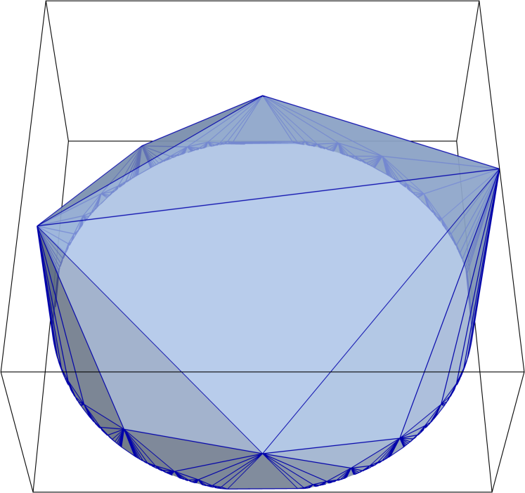
The main idea is to transfer the Epstein–Penner convex hull construction from the hyperboloid model to the hemisphere model via the projective transformation (15) (cf. Figure 11). Let denote the image of the convex hull (cf. equation (22)). The vertices of lie in the light cylinder .
The group acts by projective transformations on both the hemisphere and its equatorial disk, which is a Klein disk translated to height . Thus, the Riemann surface appears also as and as . The Delaunay decompositions of and are obtained by projecting the faces of vertically to and , respectively.
The hemisphere and the equatorial Klein disk share the unit circle at height as their circle at infinity. The th cusp of corresponds to a -orbit . A horocycle at the cusp corresponds to a -orbit , which is the image of under the transformation (15) and contains exactly one point vertically above each point in . The height of a point in depends only on the length of the corresponding horocycle in and on the point above which it lies.
Lemma 6.1.
The height of the point in above depends linearly on , i.e.,
Proof.
The point and the weight determine a unique point on the light cone . It follows from equation (17) together with equation (18), that scaling (and all the points in the -orbit of ) by results in scaling the -lengths at the th cusp by . Thus, by equation (21), modifying the weight from to changes the point to . If we go from the hyperboloid model to the hemisphere model via the transformation (15), we arrive at the point Hence we obtain . ∎
Let be an ideal triangulation of and let be the corresponding -invariant triangulation of the Klein disk at height . An ideal triangle of is also a Euclidean triangle inscribed in the unit circle. Let denote its Euclidean area. If the vertices , , of correspond to the cups , , , respectively, then the Euclidean volume of the truncated prism over with heights is
We call the polyhedral complex generated by these skew prisms, formed from all ideal triangles in , the -dome of ; see Figure 11 (right) for an illustration. The -dome depends not only on , and , but also on the group . A conjugate subgroup with has the same Riemann surface as quotient, but the -dome is transformed by the projective action of . Unless this is a rotation around the vertical axis, the volume of the transformed -dome will in general be different. As a consequence, the volume depends on the point that corresponds to the origin in the Klein model. We denote the volume of the -dome by and obtain
Note that this infinite sum has a finite value because it it is the limit of an increasing and bounded sequence. The boundedness follows from the fact that the union of orbits is bounded away from the origin [EP88], which implies that the image is bounded in height.
Lemma 6.2.
The function is linear.
Proof.
For a vertex of a triangle let denote the cusp corresponding to the -orbit of , i.e., if . We write for the multiplicity of the th cusp in the triangle , i.e., the number of vertices of with . This is a number between zero and three. By rearranging the absolutely convergent sum and invoking Lemma 6.1 we obtain
∎
Definition 6.3.
We call
the GKZ vector of the ideal triangulation .
By definition we have . The following is our hyperbolic analog of a key characterization of regular triangulations in the Euclidean setting; see [DLRS10, Lemma 5.2.14].
Proposition 6.4 (Hyperbolic Crucial Lifting Lemma).
Let be a triangulation of , and let be an arbitrary weight vector. Then the following are equivalent:
-
(i)
The triangulation refines the Delaunay decomposition .
-
(ii)
We have for all triangulations of , with equality if and only if refines as well.
Proof.
The Delaunay decomposition in the Klein disk is obtained by orthogonally projecting the upper boundary of the convex hull to the Klein disk. Thus refines if and only if the -dome of equals .
Let be an arbitrary triangulation of and let be some triangle in . The skew prism over with heights prescribed by is contained in by convexity. Furthermore, its top triangle is contained in a face of if and only if refines a cell of . It follows that the volume of the -dome of does not exceed the volume of . These two volumes coincide if and only if each triangle of refines a cell of . ∎

Definition 6.5.
For a point the secondary polyhedron of () is defined as
| (27) |
Theorem 6.6.
For each , the secondary fan is the outer normal fan of the secondary polyhedron .
Proof.
Let be a triangulation of . Denote by the the outer normal cone of the GKZ vector in . It suffices to show that
First, let . By definition . Since , it follows from Proposition 6.4 that
for all triangulations of . This shows that The other inclusion follows similarly. ∎
Example 6.7.
We continue the case of the twice punctured torus from Example 5.9. The vertices of the secondary polyhedron are the GKZ vectors of the two Delaunay triangulations and , approximately given by
Note that both and lie on the hyperplane defined by . Thus, the bounded edge of that connects the two vertices has outer normal vector . It follows that the outer normal fan of equals , indeed. Now consider the triangulation obtained by flipping one black/black edge in . The GKZ vector of that triangulation is and it lies in the relative interior of the bounded edge. Since refines the Delaunay decomposition , this illustrates the case of equality in Proposition 6.4. By further flipping a black/white edge of , we get a triangulation that does not refine any Delaunay decomposition. Note that we change the fundamental hexagon in order to illustrate this triangulation in Figure 12. The corresponding GKZ vector is and lies in the interior of the secondary polyhedron.
7. Calculating Secondary Cones, Fans and Polyhedra
We briefly want to sketch how the examples in the previous section have been computed. Our method is implemented in polymake [GJ00]. Throughout the decorated punctured Riemann surface is given in terms of Penner coordinates, i.e., some topological triangulation of together with -lengths of its edges.
The first task is to compute a secondary cone that contains a given weight vector in its relative interior. Starting out with the triangulation we can employ Week’s flip-algorithm [Wee93] to obtain a Delaunay triangulation that refines by successively flipping edges which violate the local Delaunay condition (cf. Lemma 5.4). Then the secondary cone is determined by the inequalities (25). (For a detailed analysis of the flip-algorithm, including a proof that works also for projective surfaces, see [TW16]. The case of partially decorated surfaces is discussed in [Spr17, §5].)
This allows us to compute the entire secondary fan as follows. We pick some positive weight vector and compute the secondary cone by the subroutine which we described above. Generically, is top-dimensional. Otherwise, we pick another random and try again until is top dimensional. The goal now is to compute the rest of the secondary fan via a breadth-first search in the dual graph of the secondary fan. More precisely, we maintain a queue of pairs , where is a top-dimensional secondary cone and is a facet of which does not lie in the boundary of the positive orthant. This queue is initialized with and its facets. The main loop of the algorithm picks a pair from the queue while it is not empty. For a weight vector with we pick another weight vector on the line perpendicular to which contains such that and are adjacent, i.e., they share as a common facet. It may happen that is a top-dimensional cone that we saw before. If, however, the secondary cone is new then the pairs formed by and its facets other than are added to the queue. This algorithm for computing the secondary fan of a punctured Riemann surface is very similar to the method implemented in Gfan [Jen17] for the Euclidean setting.
It remains to explain how to obtain the vertices of the secondary polyhedra. For this we loop through all top-dimensional cones of the secondary fan and compute the GKZ-vector from some Delaunay triangulation as in Definition 6.3. Clearly, that formula does not yield a finite procedure, which is why we need to be content with an approximation of .
8. Concluding Remarks and Open Questions
A standard way of measuring the combinatorial complexity of a convex polytope, or a combinatorial manifold is the face vector, or -vector for short, which records the number of cells per dimension.
Question 8.1.
What are the possible -vectors of the secondary fans and the secondary polyhedra of punctured Riemann surfaces?
Upper bounds on -vectors often translate into upper bounds on the complexity of related algorithms. Since the Delaunay triangulations correspond to secondary cones of maximal dimension, answering the previous question would, in particular, imply an upper bound on their number.
The convex hull construction of Epstein and Penner works for cusped hyperbolic manifolds of arbitrary dimension. Our construction of secondary fans and secondary polyhedra also generalizes to the higher dimensional setting in a straightforward way. Similarly, there is a version of the GKZ-construction for compact or cusped hyperbolic manifolds with marked points. This leads to the study of regular triangulations and decompositions of compact hyperbolic manifolds. Moreover, in dimension two, one may allow surfaces with cone-like singularities. While all these generalizations and extensions are fairly straightforward, many details of the constructions and some phenomena that may be observed are particular to each setting. In the present article we avoided the maximal possible generality in favor of a concise presentation of our key ideas.
Another direction for future research involves manifolds with a geometric structure that is< not metric. For example, Cooper and Long [CL15] recently generalized the Epstein–Penner construction to projective manifolds. So the following question is natural.
Question 8.2.
Do secondary fans and secondary polyhedra of projective manifolds exist?
Our construction yields a secondary polyhedron for each point in a punctured Riemann surface.
Question 8.3.
Can anything interesting be said about the dependence of the secondary polyhedron on the point ?
References
- [Aki01] Hirotaka Akiyoshi. Finiteness of polyhedral decompositions of cusped hyperbolic manifolds obtained by the Epstein-Penner’s method. Proc. Amer. Math. Soc., 129(8):2431–2439, 2001.
- [Bea95] Alan F. Beardon. The geometry of discrete groups, volume 91 of Graduate Texts in Mathematics. Springer-Verlag, New York, 1995. Corrected reprint of the 1983 original.
- [BS92] Louis J. Billera and Bernd Sturmfels. Fiber polytopes. Ann. of Math. (2), 135(3):527–549, 1992.
- [CFKP97] James W. Cannon, William J. Floyd, Richard Kenyon, and Walter R. Parry. Hyperbolic geometry. In Flavors of geometry, volume 31 of Math. Sci. Res. Inst. Publ., pages 59–115. Cambridge Univ. Press, Cambridge, 1997.
- [CL15] D. Cooper and D. D. Long. A generalization of the Epstein-Penner construction to projective manifolds. Proc. Amer. Math. Soc., 143(10):4561–4569, 2015.
- [DLRS10] Jesús A. De Loera, Jörg Rambau, and Francisco Santos. Triangulations, volume 25 of Algorithms and Computation in Mathematics. Springer-Verlag, Berlin, 2010.
- [EP88] D. B. A. Epstein and R. C. Penner. Euclidean decompositions of noncompact hyperbolic manifolds. J. Differential Geom., 27(1):67–80, 1988.
- [GJ00] Ewgenij Gawrilow and Michael Joswig. polymake: a framework for analyzing convex polytopes. In Gil Kalai and Günter M. Ziegler, editors, Polytopes — Combinatorics and Computation, pages 43–74. Birkhäuser, 2000.
- [GKZ08] I. M. Gelfand, M. M. Kapranov, and A. V. Zelevinsky. Discriminants, Resultants and Multidimensional Determinants. Birkhäuser, Boston, 2008. Reprint of the 1994 edition.
- [GLSW13] Xianfeng Gu, Feng Luo, Jian Sun, and Tianqi Wu. A discrete uniformization theorem for polyhedral surfaces. arXiv:1309.4175v1 [math.GT], 2013.
- [Jen17] Anders N. Jensen. Gfan, a software system for Gröbner fans and tropical varieties, version 0.6. Available at http://home.imf.au.dk/jensen/software/gfan/gfan.html, 2017.
- [Kap09] Michael Kapovich. Hyperbolic manifolds and discrete groups. Modern Birkhäuser Classics. Birkhäuser Boston, Inc., Boston, MA, 2009. Reprint of the 2001 edition.
- [Kat92] Svetlana Katok. Fuchsian groups. Chicago Lectures in Mathematics. University of Chicago Press, Chicago, IL, 1992.
- [Leh66] Joseph Lehner. A short course in automorphic functions. Holt, Rinehart and Winston, New York-Toronto, Ont.-London, 1966.
- [Pen87] Robert C. Penner. The decorated Teichmüller space of punctured surfaces. Comm. Math. Phys., 113(2):299–339, 1987.
- [Pen12] Robert C. Penner. Decorated Teichmüller Theory. QGM Master Class Series. European Mathematical Society, Zürich, 2012.
- [Spr17] Boris Springborn. Hyperbolic polyhedra and discrete uniformization. arXiv:1707.06848 [math.MG], 2017.
- [Thu97] William P. Thurston. Three-dimensional geometry and topology. Vol. 1, volume 35 of Princeton Mathematical Series. Princeton University Press, Princeton, NJ, 1997. Edited by Silvio Levy.
- [TW16] Stephan Tillmann and Sampson Wong. An algorithm for the Euclidean cell decomposition of a cusped strictly convex projective surface. J. Comput. Geom., 7(1):237–255, 2016.
- [Wee93] Jeffrey R. Weeks. Convex hulls and isometries of cusped hyperbolic -manifolds. Topology Appl., 52(2):127–149, 1993.