Testing $k$-monotonicity of a discrete distribution. Application to the estimation of the number of classes in a population

Abstract

We develop here several goodness-of-fit tests for testing the $k$-monotonicity of a discrete density, based on the empirical distribution of the observations. Our tests are non-parametric, easy to implement and are proved to be asymptotically of the desired level and consistent. We propose an estimator of the degree of $k$-monotonicity of the distribution based on the non-parametric goodness-of-fit tests. We apply our work to the estimation of the total number of classes in a population. A large simulation study allows to assess the performances of our procedures.

1 Introduction

The estimation of the distribution of categorical variables is an important issues in statistical research. For modeling count data parametric models or nonparametric extensions such as mixtures of Poisson distributions are very popular. An alternative to these nonparametric modelings is to consider a shape constraint on the underlying probability mass function. Such approach may be well adapted in some situations because it combines the straightforwardness of parametric models (no choice of parameter is left to the user) and the great flexibility of nonparametric estimation. Moreover shape constraint arises naturally in many frameworks such as insurance [24], reliability studies [29], epidemiology [3] or ecology [14, 15].

Several authors have considered the problem of estimating a discrete density under shape constraints. Balabdaoui et al. [5] considered the maximum-likelihood estimator under constraint of log-concavity and Balabdaoui and Jankowski [3] under constraint of unimodality. Jankowski and Wellner [23] studied the asymptotic properties of several estimators of the density under assumption of monotonicity. Durot et al. [13] proposed a least-squares estimator under convexity constraint while Giguelay [18] considered $k$-monotonicity constraint. The case $k=1$ corresponds to monotonicity, the case $k=2$ to convexity, and the more $k$ increases, the more the density is hollow.

The constraint of $k$-monotonicity is especially suitable when one aims to estimate the unknown number of classes or categories in a population. One of the main approaches to deal with that problem consists in estimating the distribution of the observed abundances for a series of classes, from which the estimation of the total number of classes is deduced. See Bunge and Fitzpatrick [10] for a review of the different approaches to deal with that problem. Durot et al. [14, 15] proposed an estimator of the total number of classes based on an estimator of the abundance distribution under the constraint of convexity. Giguelay [19] generalises their work to $k$-monotonicity. Chee and Wang [12] proposed to model the abundance distribution of species with a mixture of discrete beta distributions, such a mixture being $k$-monotone. These authors underlined that their model is particularly suitable when a population is dominated by a large number of rare species.

In order to validate the chosen model before estimating the number of classes, we propose a goodness-of-fit test for testing $k$-monotonicity. To the best of our knowledge, very few works are available for testing a shape constraint on a discrete density: Akakpo et al. [1] proposed a procedure for testing monotonicity ($k=1)$, while Durot et al. [15] and Balabdaoui et al. [7] considered the problem of testing convexity ($k=2$). The testing procedures they proposed rely on the asymptotic distribution of some distance between the empirical distribution and the estimation of the density under the shape constraint. This approach presents several difficulties. It needs the calculation of the asymptotic distribution of the test statistic under the null hypothesis which proves to be a difficult problem even for $k=2$ both from a theoretical and a computational point of view.

We develop here several goodness-of-fit tests for $k$-monotonicity of a discrete density, based on the empirical distribution of the observations. Our tests are non-parametric in the sense that there is no parametric assumption on the underlying true distribution of the observations. The procedures are easy to implement and are proved to be asymptotically of the desired level and consistent. We carry out a large simulation study in order to assess the performances of our procedures for finite sample size. From this study, it appears that the asymptotic specifications are achieved when the number of observations is very large. In order to evaluate the intrinsic difficulty of these non-parametric procedures, we compare the efficiency of our procedures to the one of parametric procedures constructed under the assumption of Poisson densities. This work is presented in Section 2.

Next, in Section 3, we propose an estimator of the degree of $k$-monotonicity of the distribution based on the non-parametric goodness-of-fit tests. We show that, if the true underlying distribution is $k$-monotone, then the probability for our estimator $\widehat{k}$ to be less than $k-1$ is smaller than the chosen level of the testing procedure. On the other way, if the true underlying distribution is $k$-monotone but not $k+1$-monotone, the probability for $\widehat{k}$ to be greater than $k+1$ tends to zero.

Finally, in Section 5, we apply our work to the estimation of the total number of classes in a population , denoted $N$, under the assumption that the abundances of the $N$ classes are i.i.d. with common distribution $p=(p_{0},p_{1},\ldots)$ where for any integer $j\leqslant 0$, $p_{j}$ is the probability to observed a class $j$ times. Generalizing the work of Durot et al. [14] we define a “$k$-monotone abundance distribution” in order to make the total number of classes identifiable. For each $k$, we are able to calculate an estimator of $N$. At the same time, using the previous testing procedures, we estimate $k$, which leads to a final estimator of $N$. This procedure is illustrated in Section 6 on three examples given in the litterature.

A small conclusion is given in Section 7 and all the proofs are postponed to Section 8.

2 Testing the $k$-monotonicity of a discrete distribution

We present $k$-monotonicity testing procedures for any discrete distribution $p$ defined on a finite support included in $\{0,\ldots,\tau\}$ for some unknown integer $\tau$. Our results may be generalised to the case $\tau=\infty$

Let us give the definition of $k$-monotonicity of a discrete distribution.

Definition 1

Let $k\geqslant 1$ and for all $j\in\mathbb{N}$, let $\Delta^{k}p_{j}$ be the $k^{{\rm th}}$ differential operator of $p$ defined as follows:

$$\Delta^{1}p_{j} = p_{j+1}-p_{j}$$

$$\Delta^{k}p_{j} = \Delta^{k-1}p_{j+1}-\Delta^{k-1}p_{j}.$$ (1)

A discrete distribution $p$ on $\mathbb{N}$ is $k$-monotone if and only if

$$\nabla^{k}p_{j}=(-1)^{k}\Delta^{k}p_{j}\geqslant 0,\mbox{for all }j\in\mathbb{N}.$$

It is easy to see that

$$\nabla^{k}p_{j}=\sum_{h=0}^{k}(-1)^{h}C_{k}^{h}p_{j+h}.$$

It can be shown, see [18], that if $p$ is $k$-monotone, then $p$ is strictly $l$-monotone for all $1\leqslant l\leqslant k-1$. Moreover $p$ can be decomposed into a mixture of polynomial distributions of order $k$ [25]. More precisely, for all integer $j\in\mathbb{N}$

$$p_{j}=\sum_{\ell\geqslant 0}\pi^{k}_{\ell}Q^{k}_{\ell}(j)$$ (2)

where

$$\pi^{k}_{\ell}=C_{k+\ell}^{k}\nabla^{k}p_{\ell}\mbox{ for all }\ell\in\mathbb{N},$$ (3)

and where $Q^{k}_{\ell}$ is the $k$-monotone distribution defined as

$$Q^{k}_{\ell}(j)=\frac{C_{k-1+\ell-j}^{k-1}}{C_{k+\ell}^{k}}I(j\leqslant\ell),$$ (4)

where $I$ denotes the indicator function.

The support of the distribution $\pi$ is the set of integers $j$ such that $\nabla^{k}p_{j}$ is strictly positive. Such integers are called the $k$-knots of $p$.

Let $X_{1},\ldots,X_{d}$ be a $d$-sample with distribution $p$ and $f$ the relative frequencies: for all $j\geqslant 0$

$$p_{j} = P(X_{i}=j)$$

$$f_{j} = \frac{1}{d}\sum_{i=1}^{d}I(X_{i}=j).$$

We propose to test the null hypothesis that $p$ is $k$-monotone considering the fact that if $\nabla^{k}p_{j}$ is negative for some $j\geqslant 0$, then $p$ is not $k$-monotone. Therefore we propose to reject the $k$-monotonicity of $p$ if one of the estimators $\nabla^{k}f_{j}$ of $\nabla^{k}p_{j}$ is negative enough.

2.1 Testing procedures and theoretical properties

Let us begin with two testing procedures. The first one, denoted P1, rejects the null hypothesis if the minimum of the $\nabla^{k}f_{j}$’s is smaller than some negative threshold, while the second one, denoted P2, rejects the null hypothesis if one of the hypothesis “$\nabla^{k}p_{j}\geqslant 0$” is rejected. Procedure P2 is a standardized version of Procedure P1.

Let us introduce the following notations:

• $\Gamma$ is the matrix with components $\Gamma_{jj^{\prime}}=-p_{j}p_{j^{\prime}}$ if $j\neq j^{\prime}$ and $\Gamma_{jj}=p_{j}(1-p_{j})$ for $0\leqslant j,j^{\prime}\leqslant\tau$, and $\Gamma^{1/2}$ its square-root such that $\Gamma^{1/2}\Gamma^{1/2}=\Gamma$.

• $A^{k}$ is the matrix whose lines $A^{kT}_{j}$ satisfy $\nabla^{k}p_{j}=A^{kT}_{j}p$ for $j=0,\ldots,\tau-1$.

• $M^{k}$ is the square-root of the matrix $A^{k}\Gamma A^{kT}$: $M^{k}M^{k}=A^{k}\Gamma A^{kT}$

• $(\mathcal{Z}_{j^{\prime}},j^{\prime}=0,\ldots\tau-1)$ are i.i.d. $\mathcal{N}(0,1)$ variates, and $\mathcal{Z}$ is the random vector with components $\mathcal{Z}_{j^{\prime}},j^{\prime}=0,\ldots\tau-1$.

• For $0<\alpha<0.5$,

  $$q^{k}_{\alpha}=\inf_{q}\left\{\mathbb{P}\left(\min_{0\leqslant j\leqslant\tau-1}\sum_{j^{\prime}=0}^{\tau-1}M^{k}_{jj^{\prime}}\mathcal{Z}_{j^{\prime}}\leqslant q\right)=\alpha\right\},$$ (5)

  $$u^{k}_{\alpha}=\max_{0\leqslant u\leqslant 1}\left\{\mathbb{P}\left(\min_{0\leqslant j\leqslant\tau-1}\left\{A_{j}^{kT}\Gamma^{1/2}\mathcal{Z}-\nu_{u}\sqrt{A^{kT}_{j}\Gamma A^{k}_{j}}\right\}\leqslant 0\right)=\alpha\right\},$$

  where $\nu_{u}$ is the $u$-quantile of a $\mathcal{N}(0,1)$ variable.

• $\widehat{\tau}$ the maximum of the support of the empirical distribution, $\widehat{\tau}=\max_{i=1,\ldots D}X_{i}$

• $\widehat{\Gamma}$, $\widehat{M}^{k}$, $\widehat{\mathcal{Z}}$, $\widehat{q}^{k}_{\alpha}$, $\widehat{u}^{k}_{\alpha}$ are defined as above with $f$ instead of $p$ and $\widehat{\tau}$ instead of $\tau$.

Testing procedures

P1

The rejection region for testing that $p$ is $k$-monotone is defined as

$$\left\{\widehat{\mathcal{T}}^{k}\leqslant\widehat{q}^{k}_{\alpha}\right\}\mbox{ where }\widehat{\mathcal{T}}^{k}=\sqrt{d}\min_{0\leqslant j\leqslant\widehat{\tau}-1}\nabla^{k}{f}_{j}.$$

Let us note that the threshold $\widehat{q}^{k}_{\alpha}$ defined above, is the $\alpha$-quantile of the conditional distribution given $X_{1},\ldots,X_{d}$ of

$$\widehat{\mathcal{U}}^{k}=\min_{0\leqslant j\leqslant\widehat{\tau}-1}\sum_{j^{\prime}=0}^{\widehat{\tau}-1}\widehat{M}^{k}_{jj^{\prime}}\widehat{\mathcal{Z}}_{j^{\prime}}.$$ (6)

It is calculated by simulation.

P2

The second procedure will reject the null hypothesis if the minimum of $\nabla^{k}f_{j}$ minus some threshold depending on $j$ is negative. Precisely the rejection region for testing that $p$ is $k$-monotone is defined as

$$\left\{\widehat{\mathcal{S}}_{\alpha}^{k}\leqslant 0\right\}\mbox{ where }\widehat{\mathcal{S}}^{k}_{\alpha}=\min_{0\leqslant j\leqslant\widehat{\tau}-1}\left\{\sqrt{d}\nabla^{k}{f}_{j}-\nu_{\widehat{u}^{k}_{\alpha}}\sqrt{A^{kT}_{j}\widehat{\Gamma}A^{k}_{j}}\right\}.$$

The quantity $\widehat{u}^{k}_{\alpha}$ is calculated by simulation.

We also propose a bootstrap procedure for calculating either the quantiles $\widehat{q}^{k}_{\alpha}$ or the $\nu_{u}$ for $u$ in a grid of values. These procedures called P1boot and P2boot are described in Section 2.4

The two following theorems give the asymptotic properties of the testing procedures. Their proof are given in Section 8.

Theorem 1

Level of the test.  
Let $p$ be a $k$-monotone distribution with finite support. The testing procedures have asymtotic level $\alpha$:

$$\lim_{d\rightarrow\infty}\mathbb{P}\left(\widehat{\mathcal{T}}^{k}\leqslant\widehat{q}^{k}_{\alpha}\right)\leqslant\;\alpha,\;\lim_{d\rightarrow\infty}\mathbb{P}\left(\widehat{\mathcal{S}}^{k}_{\alpha}\leqslant 0\right)\leqslant\;\alpha$$

If $p$ is a strictly $k$-monotone distribution with finite support, then we have the following result

P1

Let $\sigma^{k}=\max_{0\leqslant j\leqslant\tau-1}\sqrt{\sum_{j^{\prime}=0}^{\tau-1}(M^{k}_{jj^{\prime}})^{2}}$ and $\beta>0$. If the distribution $p$ satisfies the following property

$$\min_{0\leqslant j\leqslant\tau-1}\nabla^{k}p_{j}\geqslant\sqrt{\frac{2}{d}}\sigma^{k}\sqrt{\log\frac{\tau}{\beta}},$$

then

$$\lim_{d\rightarrow\infty}\mathbb{P}\left(\widehat{\mathcal{T}}^{k}\leqslant\widehat{q}^{k}_{\alpha}\right)\leqslant\beta.$$

P2

Let $\zeta_{j}^{k}=\sqrt{A_{j}^{kT}\Gamma A_{j}^{k}}$, and $\zeta^{k}=\max_{j}\zeta_{j}^{k}$, and let $\beta>0$. If the distribution $p$ satisfies the following property

$$\min_{0\leqslant j\leqslant\tau}\nabla^{k}p_{j}\geqslant\sqrt{\frac{2}{d}}\zeta^{k}\sqrt{\log\frac{\tau}{\beta}},$$

then

$$\lim_{d\rightarrow\infty}\mathbb{P}\left(\widehat{\mathcal{S}}^{k}_{\alpha}\leqslant 0\right)\leqslant\beta.$$

In particular, if the distribution $p$ is strictly $k$-monotone and satisfies the above condition for $\beta$ that tends to 0, for example $\beta=1/\sqrt{d}$, then the level of the test tends to 0.

Theorem 2

Power of the test.
Let $p$ be a $k$-monotone distribution, but not a $(k+1)$-monotone distribution and $\beta>0$.

P1

Let $\sigma^{k}=\max_{0\leqslant j\leqslant\tau-1}\sqrt{\sum_{j^{\prime}=0}^{\tau-1}(M^{k}_{jj^{\prime}})^{2}}$. If $p$ satisfies the following condition:

$$\exists j_{0},\nabla^{k+1}p_{j_{0}}+\frac{1}{\sqrt{d}}\left(\sigma^{k+1}\sqrt{2\log\frac{\tau}{\alpha}}+\zeta^{k+1}_{j_{0}}\sqrt{-2\log\beta}\right)\leqslant 0,$$

then we have the following result:

$$\lim_{d\rightarrow\infty}\mathbb{P}\left(\widehat{\mathcal{T}}^{k+1}\geqslant\widehat{q}^{k+1}_{\alpha}\right)\leqslant\beta.$$

P2

Let $\zeta_{j}^{k}=\sqrt{A_{j}^{kT}\Gamma A_{j}^{k}}$. If $p$ satisfies the following condition:

$$\exists j_{0},\;\nabla^{k+1}p_{j_{0}}+\frac{1}{\sqrt{d}}\left(\sqrt{2\log\frac{\tau}{\alpha}}+\sqrt{-2\log\beta}\right)\zeta^{k+1}_{j_{0}}\leqslant 0,$$

then we have the following result:

$$\lim_{d\rightarrow\infty}\mathbb{P}\left(\widehat{\mathcal{S}}_{\alpha}^{k}\geqslant 0\right)\leqslant\beta.$$

In order to evaluate the performances of the two testing procedures for finite sample size, we carry out a simulation study. In Section 2.2 we consider Poisson distributions with parameters chosen to ensure $k$-monotonicity, and in Section 2.3 we consider mixtures of Splines distributions.

2.2 Simulation for Poisson distributions

2.2.1 Poisson distribution and $k$-monotonicity

We carry out a simulation study, considering empirical distributions simulated according to Poisson distributions with parameters $\lambda^{h}$ chosen as follows: for all $\lambda\leqslant\lambda^{h}$ then $p\sim\mathcal{P}(\lambda)$ is at least $h$-monotone, and for all $\lambda\in\left]\lambda^{h},\lambda^{h-1}\right]$, then $p\sim\mathcal{P}(\lambda)$ is $(h-1)$-monotone but not $h$-monotone. For $h\in\{1,\ldots,10\}$ the values of $\lambda^{h}$, calculated numerically, are given at Table 1. Note that by choosing these values of $\lambda$ for our simulation study, we are in the best scenario to reject $H_{k}$ when $k=h+1$, since the Poisson distribution with parameter $\lambda^{h}$ is the most distant from the set of $k$-monotone Poisson distributions.

$h$	0	1	2	3	4	5	6	7	8	9	10
$\lambda^{h}$	2	1	0.5857	0.4157	0.3225	0.2635	0.2228	0.193	0.1703	0.1523	0.1377

Table 1: For $h\geqslant 0$, values of $\lambda^{h}$ used in the simulation study: the data are generated according to the distributions $\mathcal{P}(\lambda^{h})$.

When $\lambda>1$, the Poisson distribution $\mathcal{P}(\lambda)$ is unimodal. In the simulation study, we choose $\lambda^{0}=2$, to represent non monotone distributions. For $h\geqslant 1$, the values of $\lambda^{h}$ and the differences $\lambda^{h}-\lambda^{h+1}$ decrease with $h$, see Figure 1. Some numerical calculations show that $\lambda^{h}$ decreases approximatively as $1.13/h^{0.9}$, $\lambda^{h+1}/\lambda^{h}$ decreases as $1-0.84/(h+1)$, while $\sqrt{\lambda^{h}}-\sqrt{\lambda^{h+1}}$ decreases as $0.64/(h+1)^{1.52}$ (this last result will be usefull later on). This suggests that testing $H^{h+1}$ when $p\sim\mathcal{P}(\lambda^{h})$ will be difficult for large $h$.

Figure 1: Variation of $\lambda^{h}$ versus $h$ and fitted line in red. Fig. a: $\log\left(\lambda^{h}\right)$ versus $\log(h)$, fitted $=0.12-0.92\log(h)$. Fig. b: $\lambda^{h+1}/\lambda^{h}$ versus $1/(h+1)$, fitted $=0.99-0.84/(h+1)$. Fig. c: $\log\left(\sqrt{\lambda^{h}}-\sqrt{\lambda^{h+1}}\right)$ versus $\log(h+1)$, fitted $=-0.45-1.52\log(h+1)$.

2.2.2 Simulation study

Procedure P1

For each value of $h$, we estimate the rejection probabilities of hypotheses $H^{k}$, for $k\in\{1,\ldots,9\}$ on the basis of $500$ runs. The results for procedure P1 are given in Table 2.

For $d=1000$, $p\sim\mathcal{P}(\lambda^{h})$

	$h=10$	$h=9$	$h=8$	$h=7$	$h=6$	$h=5$	$h=4$	$h=3$	$h=2$	$h=1$	$h=0$
$k=1$	0	0	0	0	0	0	0	0	0	0.036	1
$k=2$	0	0	0	0	0	0	0	0	0.058	0.990	1
$k=3$	0	0	0	0	0	0	0	0.060	0.760	0.958	0.370
$k=4$	0	0	0	0	0	0.002	0.030	0.422	0.814	0.646	0.074
$k=5$	0	0	0	0	0	0.064	0.236	0.560	0.678	0.268	0.042
$k=6$	0	0	0	0.010	0.060	0.216	0.378	0.524	0.470	0.108	0.042
$k=7$	0	0	0.014	0.062	0.148	0.300	0.362	0.410	0.272	0.056	0.058
$k=8$	0.010	0.018	0.050	0.126	0.224	0.326	0.320	0.256	0.160	0.042	0.062
$k=9$	0.030	0.044	0.102	0.178	0.244	0.296	0.252	0.206	0.112	0.036	0.058
$k=10$	0.080	0.080	0.142	0.206	0.240	0.268	0.192	0.158	0.090	0.042	0.060

For $d=5000$, $p\sim\mathcal{P}(\lambda^{h})$ $h=10$ $h=9$ $h=8$ $h=7$ $h=6$ $h=5$ $h=4$ $h=3$ $h=2$ $h=1$ $h=0$ $k=1$ 0 0 0 0 0 0 0 0 0 0.034 1 $k=2$ 0 0 0 0 0 0 0 0 0.056 1 1 $k=3$ 0 0 0 0 0 0 0 0.062 1 1 0.992 $k=4$ 0 0 0 0 0 0 0.052 0.960 1 1 0.198 $k=5$ 0 0 0 0 0 0.062 0.766 0.994 1 0.762 0.036 $k=6$ 0 0 0 0 0.040 0.494 0.904 0.986 0.962 0.260 0.018 $k=7$ 0 0 0.002 0.056 0.370 0.748 0.910 0.948 0.694 0.092 0.036 $k=8$ 0 0.004 0.060 0.256 0.580 0.776 0.852 0.788 0.360 0.044 0.050 $k=9$ 0.006 0.070 0.156 0.434 0.650 0.738 0.746 0.564 0.166 0.040 0.050 $k=10$ 0.042 0.170 0.306 0.490 0.628 0.636 0.584 0.368 0.090 0.042 0.048

Table 2: Procedure P1: Estimated probabilities of rejecting the hypothesis $H^{k}$, for Poisson distributions with parameters $\lambda^{h}$ given at Table 1. In bold character, the probablities of rejecting $H^{k}$ with $k=h+1$, for $h\geqslant 0$. In italic character, the probablities of rejecting greater than $0.5$.

	$k=3$	$k=4$	$k=5$	$k=6$	$k=7$	$k=8$	$k=9$	$k=10$
$\sqrt{d}\nabla^{k}p_{0}$	-4.86	-7.79	-9.23	-9.52	-8.98	-7.87	-6.41	-4.79
$\sqrt{A^{kT}_{0}\Gamma A^{k}_{0}}$	2.08	3.07	4.48	6.46	9.21	13.0	18.2	25.2
$q^{k}_{\alpha}$	-3.39	-5.22	-7.34	-10.7	-15.3	-22.0	-29.9	-41.3

Table 3: For the Poisson distribution with parameters $\lambda^{2}=0.5857$, for $d=1000$, values of $\sqrt{d}\min_{j\geqslant 0}\left\{\nabla^{k}p_{j}\right\}=\sqrt{d}\nabla^{k}p_{0}$, of its standard error $\sqrt{A^{kT}_{0}\Gamma A^{k}_{0}}$ and of $q^{k}_{\alpha}$ for $\alpha=5\%$.

It appears that the level of the test based on procedure P1 is close to $\alpha$ when $k=h$ and equals 0 as soon as $k$ is smaller than $h+1$. This result confirms Theorem 1 that states that the level of the test of the hypothesis $H^{k}$ tends to 0 if the distribution is strictly $k$-monotone.

As expected, the power of the test of the hypothesis $H^{k+1}$ when $h=k$ decreases with $k$. Moreover, for a fixed value of $h$, and for $k\geqslant h+1$, the power of the test of the hypothesis $H^{k}$ first increases with $k$, then decreases with $k$. In fact, the decreasing of the power for large values of $k$ may be explained as follows: when $k$ increases, the variances of the components of $\widehat{\mathcal{T}}^{k}$ increase, and the $5\%$-quantiles of the variate $\widehat{\mathcal{U}}^{k}$ given at Equation (6) becomes strongly negative, see Table 3.

This simulation leads to the following remarks:

Remark 1

It confirms that the procedure P1 for testing $H^{k}$, when the true distribution is $(k-1)$-monotone, lacks of power when $k$ is large. For example if the true distribution is $4$-monotone, the hypothesis $H^{5}$ will not be rejected with probability greater than $0.76$ (respectively 0.23) if $d=1000$ (respectively $d=5000$).

Remark 2

It shows that the power of the test of hypothesis $H^{k}$ when the true distribution is $h$-monotone, can be small when $k-h$ is large. For example if the true distribution is convex ($h=2$), the hypothesis $H^{7}$ will not be rejected with probability greater than $0.72$ if $d=1000$. Nevertheless, let us note that the power for testing $H^{3}$ is large (it equals $0.76$ for $d=1000$).

Finally, let us note that testing the hypothesis $H^{k+j}$ for $j\geqslant 1$, when we rejected $H^{k}$ is without interest, because we know that a $(k+j)$-monotone distribution is necessarily $k$-monotone. Therefore a natural idea is to modify the procedure in order to test the hypothesis $H^{k}$ if $H^{k-1}$ is not rejected. In other words, if $H^{k-1}$ is rejected, we decide that $H^{\ell}$ is rejected for all $\ell\geqslant k$. The probabilities of not rejecting the hypotheses $H^{k}$ are estimated on the basis of $500$ runs and reported in Table 4.

For $d=1000$, $p\sim\mathcal{P}(\lambda^{h})$ $h=10$ $h=9$ $h=8$ $h=7$ $h=6$ $h=5$ $h=4$ $h=3$ $h=2$ $h=1$ $h=0$ $k=1$ 0 0 0 0 0 0 0 0 0 0.036 1 $k=2$ 0 0 0 0 0 0 0 0 0.058 0.990 1 $k=3$ 0 0 0 0 0 0 0 0.060 0.760 0.994 1 $k=4$ 0 0 0 0 0 0.002 0.030 0.422 0.826 0.994 1 $k=5$ 0 0 0 0 0 0.064 0.236 0.560 0.826 0.994 1 $k=6$ 0 0 0 0.010 0.060 0.216 0.378 0.566 0.826 0.994 1 $k=7$ 0 0 0.014 0.062 0.148 0.300 0.396 0.568 0.826 0.994 1 $k=8$ 0.010 0.018 0.050 0.126 0.224 0.330 0.398 0.568 0.826 0.994 1 $k=9$ 0.030 0.044 0.102 0.180 0.248 0.338 0.398 0.568 0.826 0.994 1 $k=10$ 0.080 0.080 0.142 0.212 0.258 0.346 0.398 0.568 0.826 0.994 1

For $d=5000$, $p\sim\mathcal{P}(\lambda^{h})$ $h=10$ $h=9$ $h=8$ $h=7$ $h=6$ $h=5$ $h=4$ $h=3$ $h=2$ $h=1$ $h=0$ $k=1$ 0 0 0 0 0 0 0 0 0 0.034 1 $k=2$ 0 0 0 0 0 0 0 0 0.056 1 1 $k=3$ 0 0 0 0 0 0 0 0.062 1 1 1 $k=4$ 0 0 0 0 0 0 0.052 0.960 1 1 1 $k=5$ 0 0 0 0 0 0.062 0.766 0.994 1 1 1 $k=6$ 0 0 0 0 0.040 0.494 0.904 0.994 1 1 1 $k=7$ 0 0 0.002 0.056 0.370 0.748 0.918 0.994 1 1 1 $k=8$ 0 0.004 0.060 0.256 0.580 0.780 0.922 0.994 1 1 1 $k=9$ 0.006 0.070 0.156 0.434 0.652 0.782 0.922 0.994 1 1 1 $k=10$ 0.042 0.170 0.306 0.494 0.664 0.782 0.922 0.994 1 1 1

Table 4: Procedure P1: Estimated probabilities of rejecting the hypothesis $H^{k}$ knowing that $H_{k-1}$ is not rejected, for Poisson distributions with parameters $\lambda^{h}$ given at Table 1. In bold character, the probablities of rejecting $H^{k}$ with $k=h+1$, for $h\geqslant 0$.

Comparison with procedures P2

The results using procedures P2 are slightly worse or equivalent to those of procedure P1, see Table 5. This is easily understandable in the case of Poisson distribution the rejection of the null hypothesis lies essentially on $\nabla^{k}p^{h}_{0}$, whatever the procedure.

For $d=1000$, $p\sim\mathcal{P}(\lambda^{h})$

	Procedure P2
	$h=10$	$h=9$	$h=8$	$h=7$	$h=6$	$h=5$	$h=4$	$h=3$	$h=2$	$h=1$	$h=0$
$k=h$	0.024	0.024	0.016	0.022	0.016	0.016	0.010	0.024	0.014	0.006
$k=h+1$		0.044	0.036	0.064	0.072	0.094	0.126	0.228	0.518	0.956	1

For $d=5000$, $p\sim\mathcal{P}(\lambda^{h})$

	Procedure P2
	$h=10$	$h=9$	$h=8$	$h=7$	$h=6$	$h=5$	$h=4$	$h=3$	$h=2$	$h=1$	$h=0$
$k=h$	0.032	0.022	0.018	0.014	0.004	0.016	0.008	0.008	0.016	0.010
$k=h+1$		0.086	0.094	0.136	0.180	0.312	0.540	0.860	1	1	1

Table 5: Procedures P2 : Estimated probabilities of rejecting $H^{h}$ and $H^{h+1}$ for Poisson distribution with parameters $\lambda^{h}$.

2.2.3 Comparison with parametric testing procedures

Our simulation study showed that the testing procedure lacks of power both when $k$ and $h$ increase. We would like to understand if this difficulty is inherent to the testing problem, or comes from a bad choice of the testing procedure. For the sake of simplicity we focus on the power when testing $H^{k}$ with $k=h+1$.

To answer our question, we will consider a parametric framework where the distribution is known to be a Poisson distribution. It is then possible to propose a parametric testing procedure for testing the $k$-monotonicity, where the null hypothesis is a simple hypothesis. This parametric framework will constitute a kind of benchmark for the performances of the test.

We propose the following parametric testing procedure: for $h\geqslant 1$, we test the null hypothesis that $p$ is at least $(h+1)$-monotone against the alternative that $p$ is $h$-monotone but not $(h+1)$-monotone. In other words, we test

$$p\sim\mathcal{P}(\lambda^{h+1})\mbox{ against }p\sim\mathcal{P}(\lambda)\mbox{ with }\lambda\in\left]\lambda^{h+1},\lambda^{h}\right],$$

assuming that $X_{1},\ldots,X_{d}$ are i.i.d. with distribution $\mathcal{P}(\lambda)$.

For this testing procedures, as well as for procedure P1 (see Theorem 2), the rate of testing is the parametric rate $1/\sqrt{d}$. Nevertheless the power depends also strongly on $k$. Instead of studying the decreasing of the power versus $k$, that depends also on $d$, we compare the efficiencies of the procedures by calculating the minimal number of observations such that the power of the test is greater that some fixed value, and study how this number increases with $k$. Let us describe how these quantities are calculated according to the testing procedure.

We denote $p=p^{h}$ the density of a Poisson distribution with parameter $\lambda^{h}$.

Efficiency for the procedure P1

Let $q_{\alpha}^{h+1}$ be defined at Equation (5) calculated for $p=p^{h+1}$ and $\tau$ chosen large enough to get $\sum_{j=0}^{\tau}p_{j}\approx 1$.

Let $M^{h+1,h}$ be the square-root of the matrix $A^{h+1}\Gamma^{h}(A^{h+1})^{T}$, where $\Gamma^{h}$ is calculated for $p=p^{h}$.

For a sample size $d$, let $\pi_{\alpha,d}^{h}$ be defined as follows:

$$\pi_{\alpha,d}^{h}=\mathbb{P}\left(\min_{0\leqslant j\leqslant\tau-1}\left\{\sqrt{d}(A_{j}^{h+1})^{T}p^{h}+\sum_{j^{\prime}=0}^{\tau-1}M_{jj^{\prime}}^{h+1,h}\mathcal{Z}_{j^{\prime}}\right\}\leqslant q_{\alpha}^{h+1}\right).$$

Following the proof of Theorem 2, it is easy to show that when $d$ is large enough, $\pi_{\alpha,d}^{h}$ approximates the power of the test of the hypothesis $H^{k}$ in $\lambda=\lambda^{h}$, with $k=h+1$:

$$\mathbb{P}_{p=p^{h}}\left(\widehat{\mathcal{T}}^{h+1}\leqslant\widehat{q}_{\alpha}^{h+1}\right)=\pi_{\alpha,d}^{h}+o_{p}(1).$$

Let $\beta>0$, for each $h$, we determine the value of $d$ for which the power of the test is greater than $1-\beta$:

$$d_{{\rm P1}}^{h}=\inf_{d}\left\{\pi_{\alpha,d}^{h}\geqslant 1-\beta\right\}.$$

The values of $\pi_{\alpha,d}^{h}$ and $d_{{\rm P1}}^{h}$ are calculated by simulation.

Efficiency for the parametric procedure

The parametric testing procedure is based on $\bar{X}$, the mean of the observations. If $p=p^{h+1}$, $d\bar{X}$ is distributed as a Poisson variable with parameter $d\lambda^{h+1}$. In what follows, this distribution will be approximated by a Gaussian distribution with mean and variance equal to $d\lambda^{h+1}$.

The null hypothesis will be rejected for large values of $\bar{X}$. More precisely, under the Gaussian approximation, we get the following results:

$$\mathbb{P}_{p=p^{h+1}}\left(\bar{X}>\lambda^{h+1}+\sqrt{\frac{\lambda^{h+1}}{d}}\nu_{1-\alpha}\right) = \alpha$$

$$\mathbb{P}_{p=p^{h}}\left(\bar{X}>\lambda^{h+1}+\sqrt{\frac{\lambda^{h+1}}{d}}\nu_{1-\alpha}\right) = 1-\Phi\left(\sqrt{\frac{d}{\lambda^{h}}}\left(\lambda^{h+1}-\lambda^{h}\right)+\sqrt{\frac{\lambda^{h+1}}{\lambda^{h}}}\nu_{1-\alpha}\right)$$

and

$$d_{{\rm P}}^{h}=\left(\frac{\sqrt{\lambda^{h}}\nu_{\beta}-\sqrt{\lambda^{h+1}}\nu_{1-\alpha}}{\lambda^{h}-\lambda^{h+1}}\right)^{2}.$$ (7)

Comparison of the two procedures

Taking $\beta=\alpha$, we compare $d_{{\rm P}}^{h}$ and $d_{{\rm P1}}^{h}$.

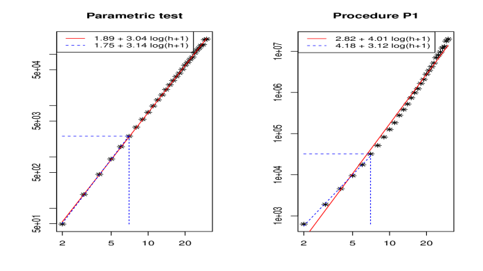
Figure 2: Variation of $d_{{\rm P}}^{h}$ (left hand side) and $d_{{\rm P1}}^{h}$ (right hand side) versus $h+1$, in $\log$-scale. The red line (respectively the dashed blue line) corresponds to a linear fit in the log-scale for $h\in{1,\ldots,29}$ (respectively $h\in{1,\ldots,6}$).

For the parametric test we get that $d_{{\rm P}}^{h}$ is of order $(h+1)^{3}$, see Figure 2. This corresponds to the order of magnitude given by Equation (7). Indeed when $\alpha=\beta$

$$d_{{\rm P}}^{h}=\frac{\nu_{1-\alpha}^{2}}{\left(\sqrt{\lambda^{h}}-\sqrt{\lambda^{h+1}}\right)^{2}},$$

which varies as $(h+1)^{3}$ as it was shown in Figure 2.

For procedure P1, the increase of $d_{{\rm P1}}^{h}$ is faster and of order $(h+1)^{4}$. This may be the price to pay when we do not know the underlying distribution.

One of the main conclusions of this study is that the use of procedure P1 needs huge values of $d$ when $h$ is large. For example, when $h=6$, around 30000 observations are needed to get a power equals to $95\%$. This result should be taken into account when one applies the method to real data sets.

If one restricts the test to values of $h$ smaller than 6, then Figure 2 shows that the growths of $d_{{\rm P1}}^{h}$ and $d_{{\rm P}}^{h}$ are of the same order, $(h+1)^{3.12}$.

Other non-parametric procedures

This section highlights the difficulty of testing $k$-monotonicity in a non-parametric setting when $k$ increases. Indeed, our conclusions are limited to the comparison with parametric testing under Poisson distributions. Morerover, other non parametric procedures could be used. For example, we could consider the least-squares estimator of $p$ under the constraint of $k$-monotonicity [18] and reject $H^{k}$ if the distance between this estimator and the empirical distribution is large, similarly to the tests proposed by [1] for the discrete monotonicity constraint and [7] for the discrete convex constraint.

Let us compare our method to the one proposed by [7], on the basis of their simulation study. They considered four distributions

$$p_{0}^{(1)} = Q^{2}_{5}$$

$$p_{0}^{(2)} = \frac{1}{6}Q^{2}_{1}+\frac{1}{6}Q^{2}_{2}+\frac{1}{3}Q^{2}_{4}+\frac{1}{3}Q^{2}_{5}$$

$$p_{1}^{(1)} = \mathcal{P}(\lambda=1.5)$$

$$p_{1}^{(2)} = Q^{2}_{5}+0.008\delta_{0}-0.008\delta_{1},$$

where $\delta_{j}$ is the Dirac distribution in $j$. For each of these distributions they estimated the rejection probabilities on the basis of 500 runs. Their testing procedure depends on the choice of a tuning parameter and we report in Table 6 the results for the best choice of this tuning parameter (see Table 1 in  [7]), as well as the results we get for testing $k=2$ with our Procedure P1.

	For $d=500$				For $d=5000$				For $d=50000$
	$p_{0}^{(1)}$	$p_{0}^{(2)}$	$p_{1}^{(1)}$	$p_{1}^{(2)}$	$p_{0}^{(1)}$	$p_{0}^{(2)}$	$p_{1}^{(1)}$	$p_{1}^{(2)}$	$p_{0}^{(1)}$	$p_{0}^{(2)}$	$p_{1}^{(1)}$	$p_{1}^{(2)}$
B. et al.	0.054	0.020	1	0.038	0.062	0.018	1	0.082	0.05	0.016	1	0.63
P1	0.046	0.034	0.956	0.034	0.052	0.040	1	0.07	0.032	0.048	1	0.36

Table 6: Comparison of the procedure proposed by Balabdaoui et al. and Procedure P1 for testing convexity.

It appears that Procedure P1 is less powerfull than the procedure based of the asymptotic distribution of the distance between $f$ and its projection on the space of convex densities. This suggests that a generalization of such a procedure for testing the $k$-monotonicity could outperform our procedure based only on the empirical distribution.
Nevertheless this is a rather difficult problem linked to the asymptotic distribution of the constraint least-squares estimator under shape constraint. The first difficulty concerns the characterization of the limit distribution. In fact, on the one hand the limit distributions is not gaussian -it is characterized by functions of brownian processes or envelope-type processes- and on the other hand the estimators are not explicit in general (see [20], Preface). For example, [4] showed that the limit distribution of the least-squares estimator of a $k$-monotone continuous distribution is a function of the primitives of a two-sided brownian bridge.
The second difficulty concerns the computation of an approximation of the limit distribution under the null hypothesis that $p$ is $k$-monotone. In particular inconsistency of the $k$-knots (the integers $j$ such that $\nabla^{k}p_{j}$ are strictly positive) may arise in the discrete case. Moreover [2] pointed out that working with sums instead of Lebesgue measure makes it more difficult to compute the limit distribution. Several authors still managed to compute an approximation of the limit distribution, [27] in the monotone case, [6] in the convex case and [5] in the log-concave case for example. In the convex case, the authors proposed a thresholding parameter to overcome inconsistency at the knots. It is likely that the same kind of difficulty should arise concerning the limit distribution of the least-squares estimator under discrete $k$-monotonicity.

2.3 Simulation for Spline distributions

As explained in Section 4.2, any $h$-monotone discrete distribution $p$ can be decomposed into a mixture of Spline distributions, see Equations (2) to (4).

We first consider Spline distributions of degree $h\in\left\{1,\ldots,6,10,20\right\}$, with one knot in $\tau$, for $\tau=15$, say $Q^{h}_{15}$. Next we consider Splines of degree $h$ with two knots, precisely the distributions

$$0.9Q^{h}_{1}+0.1Q^{h}_{15}$$

$$0.9Q^{h}_{3}+0.1Q^{h}_{15}$$

$$0.7Q^{h}_{1}+0.3Q^{h}_{15}$$

represented at Figure 3.

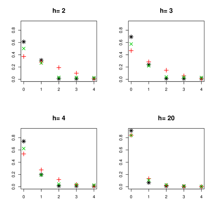
Figure 3: Spline Distributions: * for $0.9Q_{1}^{h}+0.1Q_{15}^{h}$, $+$ for $0.9Q_{3}^{h}+0.1Q_{15}^{h}$, x for $0.7Q_{1}^{h}+0.2Q_{15}^{h}$.

Spline distribution with only one knot

The results for distributions $Q^{h}_{15}$ (not reported) show that it is quite impossible to reject the null hypothesis $H^{k}$ when considering Spline distribution with one knot in $\tau=15$, at least for reasonable values of $d$. Some simple calculation may help to understand this poor performance. Let us consider the test of the hypothesis $H^{k}$ for $k=h+1$. Indeed, if $p=Q^{h}_{\tau}$, then $\nabla^{h+1}p_{j}<0$ for $j=\tau-1$ only, and

$$\nabla^{h+1}p_{\tau-1}=p_{\tau-1}-(h+1)p_{\tau}=-p_{\tau}.$$

The standard-error of its empirical estimator, $\nabla^{h+1}f_{\tau-1}$, may be approximated by

$$\sqrt{p_{\tau-1}+(h+1)^{2}p_{\tau}}/\sqrt{d}.$$

Let us consider the test of the single hypothesis “$\nabla^{h+1}p_{\tau-1}\geqslant 0$”: using the Gaussian approximation, the null hypothesis will be rejected if

$$\sqrt{d}\nabla^{h+1}f_{\tau-1}<\nu_{\alpha}\sqrt{p_{\tau-1}-(h+1)p_{\tau}}.$$

Replacing $\nabla^{h+1}f_{\tau-1}$ by $\nabla^{h+1}p_{\tau-1}$, it appears that $d$ should satisfy

$$d>\frac{\nu^{2}_{\alpha}(p_{\tau-1}+(h+1)^{2}p_{\tau})}{p^{2}_{\tau}}=\nu^{2}_{\alpha}C_{h+\tau}^{h}\left(h+(h+1)^{2}\right),$$ (8)

in order to reject “$\nabla^{h+1}p_{\tau-1}\geqslant 0$”. Clearly $d$ increases with $h$, and $\tau$ (see Table 7).

$h=1$	$h=2$	$h=3$	$h=4$	$h=5$	$h=6$
200	4000	42000	304000	1720000	8080000

Table 7: Minimum value of $d$ satisfying Equation (8) for $\tau=15$ and $\alpha=0.05$.

In practical situations, the distribution $p$ is unknown, and the test of $H^{h+1}$ lies on a multiple testing procedure, making even more difficult to reject $H^{h+1}$.

Spline distributions with 2 knots

The results for distributions of the form $\pi Q^{h}_{\ell}+(1-\pi)Q^{h}_{\tau}$ are given in Tables 8 to 10. We report the estimated probabilities of rejection for the test of the hypothesis $H^{k}$ for $k=h$ in order to estimate the level of the test, and $k=h+1$ to estimate the power.

The level of the tests are nearly equal to $5\%$. The power decreases with $h$ for all models and procedures and is greater for a mixture of spline distributions such that the first knot is close to 0, and such that the mass in the first knot is large. Nevertheless, procedure P1 gives the best results for the first and third models where the first knot appears in $j=1$, while procedure P2 performs better for the second model.

When $h$ equals 1 or 2, the power of the test is close to one for the first and third models for $d=1000$. For the second model, $d=5000$ is needed to get such a power. When $h$ increases, for example $h=5$, the difficulty for testing $H^{h+1}$ for the second model is confirmed: for $d=30000$, the power remains smaller than $10\%$.

$d=1000$

		$h=6$	$h=5$	$h=4$	$h=3$	$h=2$	$h=1$
P1	$k=h$	0.042	0.050	0.044	0.062	0.052	0.064
	$k=h+1$	0.124	0.278	0.630	0.936	1.000	1
P2	$k=h$	0.014	0.036	0.032	0.018	0.014	0.040
	$k=h+1$	0.034	0.106	0.252	0.712	0.996	1.000

$d=5000$

		$h=6$	$h=5$	$h=4$	$h=3$	$h=2$	$h=1$
P1	$k=h$	0.034	0.040	0.060	0.052	0.050	0.060
	$k=h+1$	0.360	0.816	0.990	1	1	1
P2	$k=h$	0.028	0.046	0.032	0.032	0.020	0.038
	$k=h+1$	0.126	0.566	0.952	1	1	1

$d=30000$

		$h=6$	$h=5$	$h=4$	$h=3$	$h=2$	$h=1$
P1	$k=h$	0.040	0.048	0.046	0.040	0.044	0.052
	$k=h+1$	0.964	1	1	1	1	1
P2	$k=h$	0.032	0.030	0.018	0.030	0.056	0.038
	$k=h+1$	0.818	1	1	1	1	1

Table 8: Estimated probabilities of rejecting the hypothesis $H^{k}$, for Spline distribution $p^{h}=0.9Q^{h}_{1}+0.1Q^{h}_{15}$.

$d=1000$

		$h=6$	$h=5$	$h=4$	$h=3$	$h=2$	$h=1$
P1	$k=h$	0.052	0.060	0.038	0.058	0.046	0.038
	$k=h+1$	0.044	0.056	0.050	0.048	0.212	1
P2	$k=h$	0.034	0.018	0.010	0.026	0.004	0.030
	$k=h+1$	0.030	0.022	0.058	0.100	0.508	1

$d=5000$

		$h=6$	$h=5$	$h=4$	$h=3$	$h=2$	$h=1$
P1	$k=h$	0.056	0.058	0.040	0.054	0.058	0.054
	$k=h+1$	0.060	0.048	0.038	0.070	0.998	1
P2	$k=h$	0.028	0.034	0.036	0.018	0.022	0.050
	$k=h+1$	0.042	0.050	0.080	0.496	1	1

$d=30000$

		$h=6$	$h=5$	$h=4$	$h=3$	$h=2$	$h=1$
P1	$k=h$	0.040	0.046	0.052	0.044	0.034	0.046
	$k=h+1$	0.040	0.046	0.060	0.964	1	1
P2	$k=h$	0.036	0.044	0.044	0.034	0.046	0.058
	$k=h+1$	0.042	0.088	0.518	1	1	1

Table 9: Estimated probabilities of rejecting the hypothesis $H^{k}$, for Spline distribution $p^{h}=0.9Q^{h}_{3}+0.1Q^{h}_{15}$.

$d=1000$

		$h=6$	$h=5$	$h=4$	$h=3$	$h=2$	$h=1$
P1	$k=h$	0.048	0.040	0.048	0.052	0.068	0.050
	$k=h+1$	0.072	0.106	0.298	0.716	0.998	1
P2	$k=h$	0.028	0.022	0.046	0.024	0.030	0.052
	$k=h+1$	0.028	0.034	0.126	0.354	0.938	1

$d=5000$

		$h=6$	$h=5$	$h=4$	$h=3$	$h=2$	$h=1$
P1	$k=h$	0.036	0.040	0.048	0.052	0.054	0.030
	$k=h+1$	0.132	0.312	0.802	1	1	1
P2	$k=h$	0.022	0.042	0.036	0.034	0.036	0.026
	$k=h+1$	0.042	0.134	0.492	0.990	1	1

$d=30000$

		$h=6$	$h=5$	$h=4$	$h=3$	$h=2$	$h=1$
P1	$k=h$	0.036	0.026	0.052	0.032	0.046	0.054
	$k=h+1$	0.414	0.942	1	1	1	1
P2	$k=h$	0.042	0.030	0.024	0.044	0.038	0.058
	$k=h+1$	0.180	0.770	1	1	1	1

Table 10: Estimated probabilities of rejecting the hypothesis $H^{k}$, for Spline distribution $p^{h}=0.7Q^{h}_{1}+0.3Q^{h}_{15}$.

2.4 Comparison with the bootstrap procedure

Let us describe the bootstrap procedure for estimating the quantities $q_{\alpha}^{k}$ and $u_{\alpha}^{k}$. Let $(X_{1}^{*},\ldots,X_{d}^{*})$ be a $d$-sample distributed according to the empirical distribution of $(X_{1},\ldots,X_{d})$, and let $f_{j}^{*},j=0,\ldots,\tau^{*}$ be the empirical estimator of the bootstrap distribution. Then

$$q^{*k}_{\alpha}=\inf_{q}\left\{\mathbb{P}_{X}\left(\min_{0\leqslant j\leqslant\widehat{\tau}-1}\sqrt{d}\nabla^{k}(f_{j}^{*}-f_{j})\leqslant q\right)\right\},$$

where $\mathbb{P}_{X}$ denotes the conditional distribution given $(X_{1},\ldots,X_{d})$.

For estimating $u^{k}_{\alpha}$ we use a double bootstrap. For a given $u$ and for $0\leqslant j\leqslant\widehat{\tau}-1$, let $\nu^{*}_{j,u}$ be defined as follows:

$$\nu^{*}_{j,u}=\inf_{\nu}\left\{\mathbb{P}_{X}\left(\sqrt{d}\nabla^{k}(f_{j}^{*}-f_{j})\leqslant\nu\sqrt{A_{j}^{kT}\widehat{\Gamma}A_{j}^{k}}\right)=u\right\}$$

Next let $(X_{1}^{**},\ldots,X_{d}^{**})$ be a $d$-sample distributed according to the empirical distribution of $(X_{1},\ldots,X_{d})$, independant of $(X_{1}^{*},\ldots,X_{d}^{*})$, and let $f_{j}^{**},j=1,\ldots,\tau^{**}$ be the empirical frequencies. The bootstrap estimator of $u_{\alpha}$ is defined as follows:

$$u^{*k}_{\alpha}=\max_{0\leqslant u\leqslant 1}\left\{\mathbb{P}_{X}\left(\min_{0\leqslant j\leqslant\widehat{\tau}-1}\left\{\sqrt{d}\nabla^{k}(f_{j}^{**}-f_{j})-\nu^{*}_{j,u}\sqrt{A_{j}^{kT}\widehat{\Gamma}A_{j}^{k}}\right\}\leqslant 0\right)=\alpha\right\}.$$

The results (not shown) are equivalent to those of procedures P1 and P2.

Although the validity of the boostrap procedure, like our procedures P1 and P2, lies on asymptotic arguments, we could have expected a different behaviour of the bootstrap procedure, because bootstrap does not use the approximation of the empirical distribution by the Gaussian distribution for practical calculation. This is clearly not the case, may be because our simulation study consider values of the sample size $d$ large enough to guarantee that the distribution of the empirical frequencies is closed to the Gaussian approximation.

3 Estimating the degree of monotonicity of $p$

3.1 Estimator and asymptotic properties

We propose a procedure for estimating $k$, the degree of monotonicity of $p$, based on the testing procedures described in the previous section.

For some $\alpha$ and $k_{\max}$, we define $\widehat{k}_{\alpha}$ as follows

• if there exists $1\leqslant\ell\leqslant k_{\max}$ such that $H^{\ell}$ is rejected, then

  $$\widehat{k}_{\alpha}=\inf_{1\leqslant\ell\leqslant k_{\max}}\left\{H^{\ell}\mbox{ is rejected at level }\alpha\right\}-1$$

• if not, $\widehat{k}_{\alpha}=k_{\max}$.

We show that $\widehat{k}_{\alpha}$ is asymptotically close to $k$.

Theorem 3

Let $p$ be a $k$-monotone distribution and let $\widehat{k}_{\alpha}$ be defined as above. For all $\ell\geqslant 1$, let $\sigma^{\ell}$ and $\zeta^{\ell}$ be defined as in Theorem 1. According to the testing procedure for calculating $\widehat{k}$, let us assume that the following property is statisfied:

P1

If for all $1\leqslant\ell\leqslant k-2$,

$$\min_{0\leqslant j\leqslant\tau-1}\nabla^{\ell}p_{j}\geqslant\sqrt{\frac{2}{d}}\sigma^{\ell}\sqrt{\log(\tau)+\frac{1}{2}\log(d)},$$

P2

If for all $1\leqslant\ell\leqslant k-2$,

$$\min_{0\leqslant j\leqslant\tau-1}\nabla^{\ell}p_{j}\geqslant\sqrt{\frac{2}{d}}\zeta^{\ell}\sqrt{\log(\tau)+\frac{1}{2}\log(d)},$$ (9)

then

$$\lim_{d\rightarrow\infty}\mathbb{P}\left(\widehat{k}_{\alpha}\leqslant k-1\right)\leqslant\alpha$$

If $k\leqslant k_{\max}-1$ and if $p$ satisfies the following property:

P1

$$\exists j_{0},\nabla^{k+1}p_{j_{0}}+\frac{1}{\sqrt{d}}\left(\sigma^{k}\sqrt{\log\frac{\tau}{\alpha}}+\zeta^{k}_{j_{0}}\sqrt{-2\log\frac{k_{\max}-k}{\sqrt{d}}}\right)\leqslant 0,$$ (10)

P2

$$\exists j_{0},\nabla^{k+1}p_{j_{0}}+\frac{1}{\sqrt{d}}\left(\sqrt{\log\frac{\tau}{\alpha}}+\sqrt{-2\log\frac{k_{\max}-k}{\sqrt{d}}}\right)\zeta^{k+1}_{j_{0}}\leqslant 0,$$ (11)

then

$$\lim_{d\rightarrow\infty}\mathbb{P}\left(\widehat{k}_{\alpha}\geqslant k+1\right)=0.$$

This theorem, shown in Section 8, claims that if $p$ is $k$-monotone, then the probability that $\widehat{k}_{\alpha}\leqslant k-1$ is asymptotically smaller than $\alpha$. Moreover if $p$ is far enough from $(k+1)$-monotone densities, then the probability that $\widehat{k}_{\alpha}\geqslant k+1$ tends to zero.

3.2 Simulation study

The properties of $\widehat{k}$ for $k_{\max}=6$ are assessed on the basis of the simulation study presented before. The results are given at Tables 11 to 13. They are reported for models whose degree of monotonicity is smaller than 5, when using the procedure that proved to maximise the power in the simulation study presented in the previous Section.

Let $h$ be the true degree of monotonicity of the distribution $p$. From these results, we deduce that

• Probability to underestimate $h$ when $p$ is $h$-monotone.

  The estimator $\widehat{k}_{\alpha}$ equals $h-1$ in nearly $5\%$ of the runs. When $h\geqslant 2$, the number of runs for which $\widehat{k}_{\alpha}\leqslant h-2$ is 0. This result confirms the first part of Theorem 3, see Equation (9).

• Probability to over estimate $h$ when $p$ is $h$-monotone.

  This probability is linked with the power of the test: if the test has a low power, the degree of monotonicity will be overestimated. When $h$ increases, the probability to get $\widehat{k}_{\alpha}\geqslant h+1$, and in particular $\widehat{k}_{\alpha}=k_{\max}$, increases. This overestimation decreases with $d$. For the spline distributions, if $d=5000$ the results are correct for $h\leqslant 3$.

	$d=1000$					$d=5000$					$d=30000$
$h$	$5$	$4$	$3$	$2$	$1$	$5$	$4$	$3$	$2$	$1$	$5$	$4$	$3$	$2$	$1$
$\widehat{k}$	5.77	5.27	4.42	2.68	0.99	5.50	4.30	3.00	1.94	0.92	4.97	3.96	2.93	1.96	0.97
0	0	0	0	0	2 0	0	0	0	0	2.8	0	0	0	0	3.2
1	0	0	0	3.4	97.6	0	0	0	5.6	97.2	0	0	0	4.4	96.8
2	0	0	4	74.8	0.2	0	0	5.6	94.4	0	0	0	7.2	95.6	0
3	0	4.4	36.6	5.4	0	0	4.2	90	0	0	0	4.4	92.8	0	0
4	5	24.8	16	0	0	4	70.8	3.6	0	0	4.4	95.6	0	0	0
5	12.6	10	0.6	0	0	41.8	16.2	0	0	0	94.6	0	0	0	0
6	82.4	60.8	42.8	16.4	0.2	54.2	8.8	0.8	0	0	1	0	0	0	0

Table 11: For Poisson distributions with parameters $\lambda^{h}$ given at Table 1: Estimated degree of monotonicity with procedure P1 and $\alpha=5\%$. For each value of $d$, the first row of the table gives $h$, the second the mean of $\widehat{k}_{\alpha}$ estimated over 500 runs, the following rows give the histogram of the estimated values of $\widehat{k}_{\alpha}$ (as $100\times$ percentages).

	$d=1000$					$d=5000$					$d=30000$
$h$	$5$	$4$	$3$	$2$	$1$	$5$	$4$	$3$	$2$	$1$	$5$	$4$	$3$	$2$	$1$
$\widehat{k}$	5.67	4.48	3.00	1.95	0.94	5.14	3.95	2.95	1.95	0.94	4.95	3.95	2.96	1.96	0.95
0	0	0	0	0	6.4	0	0	0	0	6	0	0	0	0	5.2
1	0	0	0	5.2	93.6	0	0	0	5	94	0	0	0	4.4	94.8
2	0	0	6.2	94.8	0	0	0	5.2	95	0	0	0	4	95.6	0
3	0	4.4	87.4	0	0	1.6	1.6	68.8	0.4	0	0	4.6	96	0	0
4	5	58.6	6.4	0	0	1	23.2	26.8	0	0	4.8	95.4	0	0	0
5	22.8	21.2	0	0	0	7.2	28.2	1.6	0	0	95.2	0	0	0	0
6	72.2	15.8	0	0	0	87.8	45	0.4	0	0	0	0	0	0	0

Table 12: For Spline distributions with two knots defined as $0.9Q^{h}_{1}+0.1Q^{h}_{15}$: Estimated degree of monotonicity with procedure P1 and $\alpha=5\%$. For each value of $d$, the first row of the table gives $h$, the second the mean of $\widehat{k}_{\alpha}$ estimated over 500 runs, the following rows give the histogram of the estimated values of $\widehat{k}_{\alpha}$ (as $100\times$ percentages).

	$d=1000$					$d=5000$					$d=30000$
$h$	$5$	$4$	$3$	$2$	$1$	$5$	$4$	$3$	$2$	$1$	$5$	$4$	$3$	$2$	$1$
$\widehat{k}$	5.90	5.78	5.47	2.71	0.97	5.83	5.73	3.89	1.97	0.95	5.11	3.95	2.94	1.96	0.94
0	0.2	0.8	1.2	0.4	3	0	0	0	0	4.6	0	0	0	0	5.8
1	0	0	0	0.4	97	0	0.6	1.6	3.2	95.4	0	0.4	1.6	3.8	94.2
2	0.2	0.8	2.4	50.4	0	2.2	1.8	1.4	96.8	0	2.2	1.2	3	96.2	0
3	2.4	3	7	39.2	0	1.6	1.8	97	0	0	1.8	1	95.4	0	0
4	0.2	2.4	6.8	2.8	0	0.6	80.6	0	0	0	0.6	97.4	0	0	0
5	0.8	0.4	2	0.2	0	18	11.8	0	0	0	73.4	0	0	0	0
6	96.2	92.6	81.1	6.6	0	77.6	3.4	0	0	0	22	0	0	0	0

Table 13: For Spline distributions with two knots defined as $0.9Q^{h}_{3}+0.1Q^{h}_{15}$: Estimated degree of monotonicity with procedure P2 and $\alpha=5\%$. For each value of $d$, the first row of the table gives $h$, the second the mean of $\widehat{k}_{\alpha}$ estimated over 500 runs, the following rows give the histogram of the estimated values of $\widehat{k}_{\alpha}$ (as $100\times$ percentages).

4 Number of classes in a population

Let us now consider the case where the total number of classes in a population is unknown, and where we aim at estimating this number based on the abundances that are observed for a series of classes. The problem is then to estimate the number of unobserved classes.

This problem was first raised in the context of ecology for estimating species richness of a population and traces back to Fisher et al. [17]. Nevertheless it also occurs in a wide variety of domains, as in social and medical sciences, epidemiology, computer science, …. Since the contribution of Fisher et al., many publications have considered this problem proposing different statistical modelings and estimators. A presentation of these different approaches was given by Bunge and Fitzpatrick [10] for example. A more recent short review can be found in [14], see also [8].

In this section, we first describe the observations and the statistical modeling, making thus the link between the $k$-monotonicity of the abundance distribution of the classes, and the estimator of the number of total classes. Then we carry out a simulation study in order to assess the properties of our estimator, and finally we consider three real case studies.

4.1 The observations

Suppose that the population is composed of $N$ classes and for $i=1\dots N$, denote by $A_{i}$ the abundance (that is the number of observed individuals) of class $i$ and by $S_{j}$ the number of classes with abundance $j$ in a sample. The total number of observed classes is $D=\sum_{j\geqslant 1}S_{j}$ whereas $S_{0}$ is the number of unobserved classes. The total number of classes is $N=S_{0}+D$ and, because $D$ is observed, the estimation of $N$ amounts to the estimation of $S_{0}$. We will denote by $n$ the sample size: $n=\sum_{i}A_{i}=\sum_{j}jS_{j}$.

We assume that the $A_{i}$’s are independent variables with the same distribution $p=(p_{0},p_{1},\dots,p_{n})$, called the abundance distribution.

As only classes that are present in the sample can be counted, classes for which $A_{i}=0$ are not observed. Thus, we only observe the zero-truncated counts $X_{1},\dots,X_{D}$, where $X_{i}$ is the abundance of the $i$-th observed classes in the sample. As it is shown by [14] (lemma 1 of the on line supporting information), $D\sim\mbox{Bin}(N,1-p_{0})$, and conditionally on $D$, $X_{1},\dots,X_{D}$ are i.i.d. random variables with distribution $p^{+}$ defined by

$$p^{+}_{j}=\frac{p_{j}}{1-p_{0}},\mbox{ for all integers }j\geqslant 1.$$ (12)

Therefore we propose to estimate $N$ by

$$\widehat{N}=\frac{D}{1-\widehat{p}_{0}},$$ (13)

where $\widehat{p}_{0}$ is an estimator of $p_{0}$.

The problem comes to estimate $p_{0}$. As we observe $X_{1},\dots,X_{D}$ from distribution $p^{+}$, we are able to estimate $p^{+}$. Nevertheless, identifiability conditions are needed to infer $p_{0}$ from the estimation of $p^{+}$. This is the object of the following section.

4.2 The assumption of a $k$-monotone abundance distribution

To make $p_{0}$, and thus $N$, identifiable, we propose a nonparametric modeling of $p$, assuming that $p$ is a discrete $k$-monotone abundance distribution, as defined in Section 2. In particular, we know that $p$ is written as a mixture of distribution $Q_{\ell}^{k}$: for all $j\in\mathbb{N}$, $p_{j}=\sum_{\ell\geqslant 0}\pi_{\ell}^{k}Q_{\ell}^{k}(j)$.

Our interpretation of this mixture is that the set of classes is separated into groups, each class having probability $\pi^{k}_{\ell}$ to belong to the group $\ell$ of classes, and the abundance distribution of all classes in the group $\ell$ is the distribution $Q^{k}_{\ell}$. As the first component $Q_{0}^{k}$ is a Dirac mass at 0, it refers to classes for which the only abundance that could be observed is 0. This group simply defines absent classes, and therefore $\pi^{k}_{0}$ has to be zero in an abundance distribution. This leads to the following definition.

Definition of a $k$-monotone abundance distribution:

The distribution $p$ on $\mathbb{N}$ is a $k$-monotone abundance distribution if there exist positive weights $\pi^{k}_{\ell}$ satisfying $\sum_{\ell\geqslant 1}\pi^{k}_{\ell}=1$, such that $p_{j}=\sum_{\ell\geqslant 1}\pi^{k}_{\ell}Q^{k}_{\ell}(j)$ for all integers $j\geqslant 0$.

In the following, we assume that the abundance distribution $p$ is a $k$-monotone abundance distribution. It then follows from (3) that $\pi^{k}_{0}=\nabla^{k}p_{0}=0$, or equivalently, that

$$\frac{1}{1-p_{0}}=1-\sum_{h=1}^{k}(-1)^{h}C_{k}^{h}p^{+}_{h},$$ (14)

where $p^{+}$ is the zero-truncated distribution defined by (12).

The distribution $p^{+}$ is identifiable since we observe $X_{1},\dots,X_{D}$ which are i.i.d. with distribution $p^{+}$ conditional on $D$. Therefore, it follows from (14) that $1-p_{0}$ is identifiable and because $D\sim\mbox{Bin}(N,1-p_{0})$, we conclude that $N$ also is identifiable. This shows that our assumption is sufficient to avoid identifiability problems. We will see how to estimate $p_{0}$ in the following section.

Let us remark that $\nabla^{k}p_{0}=0$ is equivalent to

$$p_{0} = -\sum_{h=1}^{k}(-1)^{h}C_{k}^{h}p_{h}$$

$$= -\sum_{h=1}^{k-1}(-1)^{h}C_{k-1}^{h}p_{h}-\nabla^{k}p_{0}+\nabla^{k-1}p_{0}$$

$$= -\sum_{h=1}^{k-1}(-1)^{h}C_{k-1}^{h}p_{h}+\nabla^{k-1}p_{1},$$

the last equality being deduced from the definition of $\Delta^{k}$ given at Equation (1). Therefore if we denote by $p_{0}^{k}$ the value of $p_{0}$ under the assumption that $p$ is a $k$-monotone abundance distribution, then

$$p_{0}^{k}=p_{0}^{k-1}+\nabla^{k-1}p_{1}>p_{0}^{k-1},$$

because $p$ is strictly $(k-1)$-monotone. Therefore, the mass in 0 of $p$ increases with $k$ when $p$ is assumed to be a $k$-monotone abundance distribution.

5 Estimating the number of classes

In order to estimate $N$, we first build an estimator for $1/(1-p_{0})$ based on Equation (14) and then apply Equation (13).

5.1 Estimator based on the relative frequencies

For all $j\geqslant 1$, the empirical estimator (which is the more commonly used estimator for a discrete distribution) of $p^{+}_{j}$ is $f_{j}=S_{j}/D$. Using this estimator in (13) leads to the estimator

$$\widehat{N^{k}}=D-\sum_{h=1}^{k}(-1)^{h}C_{k}^{h}S_{h}$$ (15)

Let $\widehat{s}^{k}$ be defined as follows

$$\widehat{s}^{k}=\sqrt{\sum_{h=1}^{k}\left((-1)^{h+1}+C_{k}^{h}\right)C_{k}^{h}S_{h}}.$$

If $\widehat{s}^{k}\neq 0$, one can derive from the central limit theorem that

$$\frac{\widehat{N}_{k}-N}{\widehat{s}^{k}}\mbox{ converges in law to }\mathbb{N}(0,1).$$

Let us give the following remarks:

Remark 3

If the empirical estimator of $p^{+}$ is far from being $k$-monotone, then the quantity $\sum_{h=1}^{k}(-1)^{h}C_{k}^{h}S_{h}$ may be positive. Clearly the estimator of $N$ is expected to be greater than $D$ (or equal). Therefore, for a given $k$, the method can be applied only if $\sum_{h=1}^{k}(-1)^{h}C_{k}^{h}S_{h}\leqslant 0$. This condition will guarantee that $\widehat{s}^{k}$ is well defined. For example, if we choose $k=2$, the empirical distribution should statisfy $2S_{1}-S_{2}\geqslant 0$ and $\widehat{s}^{k}=\sqrt{6S_{1}}$.

Remark 4

The bias and variance of $\widehat{N}^{k}$ can be easily calculated: (see Section 8.4)

$$\mathbb{E}\left(\widehat{N}^{k}\right) = N-N\nabla^{k}p_{0}$$

$$\mathbb{V}\left(\widehat{N}^{k}/\sqrt{N}\right) = p_{0}+\sum_{h=1}^{k}\left(C_{k}^{h}\right)^{2}p_{h}-\left(\nabla^{k}p_{0}\right)^{2}$$

If $p$ is a $k$-monotone abundance distribution, then $\nabla^{k}p_{0}=0$, $\widehat{N}^{k}$ has no bias and

$$\mathbb{V}\left(\widehat{N}^{k}/\sqrt{N}\right)=p_{0}+\sum_{h=1}^{k}\left(C_{k}^{h}\right)^{2}p_{h}=\sum_{h=0}^{k}\left(C_{k}^{h}\right)^{2}p_{h}.$$

In that case, the variance of $\widehat{N}^{k}$ increases with $k$.

Remark 5

Let us assume now that $p$ is a $k$-monotone abundance distribution, but we estimate $N$ under the assumption that $p$ is a $k-j$-abundance distribution. Then $\mathbb{E}\left(\widehat{N}^{k-j}\right)=N(1-\nabla^{k-j}p_{0})$. As

$$\nabla^{k-j}p_{0}=\nabla^{k}p_{0}+\sum_{h=0}^{j-1}\nabla^{k-j-h}p_{1}\mbox{ if }1\leqslant j\leqslant k-1,$$

$\nabla^{k}p_{0}=0$ and $\nabla^{k-j-h}p_{1}>0$ (recall that $k$-monotone distributions are strictly $(k-j)$-monotone), we get that $N$ is under-estimated.

Remark 6

If we estimate $N$ under the assumption that $p$ is a $(k+j)$-abundance distribution, then $\mathbb{E}\left(\widehat{N}^{k+j}\right)=N(1-\nabla^{k+j}p_{0})$ where

$$\nabla^{k+j}p_{0}=-\sum_{h=1}^{j}\nabla^{k+j-h}p_{1}\mbox{ if }j\geqslant 1.$$

In that case the estimator of $N$ is biased. If $j=1$, $\nabla^{k+j}p_{0}=-\nabla^{k}p_{1}$ which is negative or null, and $N$ is over-estimated.

5.2 Estimator based of the constrained least-squares estimator of $p^{+}$

The empirical estimator may be non $k$-monotone whereas under our assumptions, $p^{+}=(p^{+}_{1},p^{+}_{2},\ldots)$ is a $k$-monotone density. Hence, in addition to the empirical estimator $f=(f_{1},f_{2},\ldots)$, we consider an estimator that takes into account the constraint of $k$-monotonicity. Precisely, we consider the constrained least-squares estimator $\widetilde{p^{+}}$ of $p^{+}$ defined as follows:

$$\widetilde{p^{+}}=\mbox{arg}\min\left\{\sum_{j\geqslant 1}(q_{j}-f_{j})^{2},q=(q_{1},q_{2},\ldots),q\mbox{ a }k\mbox{-monotone distribution}\right\}.$$ (16)

Existence and uniqueness of $\widetilde{p^{+}}$ was studied by [18]. Note that this reference considers $k$-monotone distributions on $\mathbb{N}$ whereas we are interested here in $k$-monotone distributions on $\mathbb{N}\backslash\{0\}$, but considering the shifted distribution $p^{+}_{j+1}$ for $j\geqslant 0$, which is $k$-monotone on $\mathbb{N}$, and the corresponding shifted estimators $f_{j+1}$ and $\widetilde{p^{+}}_{j+1}$ allows to put our framework into that of [18], including the computation of the estimator. In that paper the author gives a characterization of the estimator based on the decomposition of $k$-monotone distributions as mixtures of spline functions. She showes that the least-squares estimator under the constraint of $k$-monotonicity is closer (with respect to the the $\ell^{2}$-loss) to any $k$-monotone distribution than the empirical distribution is. Therefore, one could expect that if $p^{+}$ is $k$-monotone, $\widetilde{p^{+}}^{k}$ will give better results, at least from the point of view of the $\ell^{2}$-loss, than the empirical distribution $f$. Moreover, the author implements the estimator using an exact iterative algorithm inspired by the Support Reduction Algorithm described in [21] and discusses a practical stopping criterion.

Finally it remains to estimate $N$ by

$$\widetilde{N}^{k}=D\left(1-\sum_{h=1}^{k}(-1)^{h}C_{k}^{h}\widetilde{p^{+}}^{k}_{h}\right).$$ (17)

5.3 Estimating the degree of monotonicity of $p^{+}$

For a given integer $k$, assuming that the distribution $p$ is a $k$-abundance distribution, we propose two estimators of $N$, $\widehat{N}^{k}$, see (15), and $\widetilde{N}^{k}$, see (17). In practical cases, we do not know the degree of monotonicity of $p$. Because we observe $X_{1},\ldots,X_{D}$ with distribution $p^{+}$, we propose to estimate the degree of monotonicity of $p^{+}$, using the method described in Section 3. Actually the degrees of monotonicity of $p$ and $p^{+}$ are not necessarily equal: we know that if $p$ is $k$-monotone then $p^{+}$ is at least $k$-monotone, but to relate the degree of monotony of $p^{+}$ to the one of $p$, we need an additional assumption on $p$. Precisely we assume that $p$ is a $k$-monotone abundance distribution, $p$ is not $(k+1)$-monotone and $\nabla^{k+1}_{j_{0}}<0$ for some $j_{0}\geqslant 1$. For example, the distributions $p^{h}=\mathcal{P}(\lambda^{h}),h\leqslant 1$ defined at Section 2.2.1 and Table 1, satisfy

$$\nabla^{h}p_{0} \approx 0$$

$$\nabla^{h}p_{j} > 0\mbox{ for all }j\geqslant 1$$

$$\nabla^{h+1}p_{0} < 0$$

$$\nabla^{h+1}p_{j} \geqslant 0\mbox{ for all }j\geqslant 1.$$

It comes that they do not satisfy the assumptions allowing to deduce the degree of monotonicity of $p$ from the one of $p^{+}$.

To sum up, we propose a procedure in two steps: at the first step we estimate the degree of monotonicity of $p^{+}$ using the procedure described at Section 3. Let us denote by $\widehat{k}$ this estimator. At the second step, we calculate $\widehat{N}=\widehat{N}^{\widehat{k}}$ and $\widetilde{N}=\widetilde{N}^{\widehat{k}}$. We assess the performances of this procedure by simulation.

5.4 Simulation experiment

We construct the distributions $p$ as follows: we choose a distribution $p^{+}=(p^{+}_{1},p^{+}_{2},\ldots)$ such that $p^{+}$ is $k$-monotone but not $(k+1)$-monotone on the set of integers greater than 1. Then we calculate $p$ such that $p_{0}$ satisfies Equation (14), and for all $j\geqslant 1$, $p_{j}=(1-p_{0})p^{+}_{j}$.

Given $N$ and $p^{+}$, a simulation consists in two steps: first we draw one realization of $D$ distributed as a $\mathcal{B}(N,1-p_{0})$, then we draw $D$ realizations $X_{1},\ldots,X_{D}$ distributed as $p^{+}$. From this simulated sample, we estimate $p^{+}$ either by the empirical dstribution $f$ or by the least-squares estimator under the constraint of $k$-monotonicity, see Equation (16).

We choose three values of $N$, $N=1000,5000,30000$, and five distributions $p^{+}$, denoted $p^{+,h}$, such that $p^{+,h}_{j}=p^{h}_{j-1}$ for $j\geqslant 1$ and for $h=\left\{1,\ldots,5\right\}$ (see Section 2.2.1 and Table 1 for the definition of $p^{h}$).

5.4.1 Comparison of the estimators $\widehat{N}^{k}$ and $\widetilde{N}^{k}$

The calculation of $\widetilde{N}^{k}$ lies on the least-squares estimator of $p^{+}$ under the constraint of $k$-monotonicity. For $k=\left\{2,3,4\right\}$ the algorithm for estimating $p^{+}$ is available in the R-package pkmon on the Comprehensive R Archive Network. For $k=1$, we used the algorithm developped by [28].

For each simulation we calculate $\widehat{k}$ for $k_{\max}=4$ using Procedure P1, $\widehat{N}^{k}$ and $\widetilde{N}^{k}$ for each $k=\left\{1,\ldots,4\right\}$, and $\widehat{N}=\widehat{N}^{\widehat{k}}$ and $\widetilde{N}=\widetilde{N}^{\widehat{k}}$. We report their expectation and prediction error estimated on the basis of $S=500$ simulations. Precisely, if $\widehat{N}^{k}_{s}$ is the estimation of $N$ at simulation $s$, we calculate

$$\mathrm{PE}(\widehat{N}^{k})=\frac{1}{S}\sum_{s}(\widehat{N}^{k}_{s}-N)^{2}.$$

We report in Table 14 $\widehat{N}^{k}_{\bullet}$, the mean of the $\widehat{N}^{k}_{s}$’s and $100\sqrt{\mathrm{PE}(\widehat{N}^{k})}/N$, as well as $\widetilde{N}^{k}_{\bullet}$ and $100\sqrt{\mathrm{PE}(\widetilde{N}^{k})}/N$. The bold values correspond to the cases where the estimation of $N$ is carried out assuming that the degree of monotonicity of the truncated distribution is known: $k=h$. The exponent denotes how many simulations failed to give the result. This may happen in the following situations:
- The estimator $\widehat{N}^{k}$ can be calculated only if $\sum_{j=1}^{k}(-1)^{j}C_{k}^{j}S_{j}$ is positive (see Remark 3). For example when $N=1000$, $k=3$, $h=1$ this condition was not satisfied in 11 simulations over 500. If $k=4$, there is no result because the condition was not satisfied in more than 1 simulation over 2. Note that this condition is always satisfied for $\sum_{j=1}^{k}(-1)^{h}C_{k}^{j}\widetilde{p^{+}_{j}}^{k}$ because $\widetilde{p^{+}}$ is $k$-monotone.
- The algorithm for calculationg $\widetilde{N}^{k}$ may fail to converge for some simulation. For example when $N=1000$, $k=4$, $h=3$ or $h=4$ this happened 10 times.
-The estimator $\widehat{k}$ may equal 0, in particular when $h=1$: this is expected in about $5\%$ of the simulations (the aymptotic level of the testing procedure). When $N=1000$, and $h=1$ this happenned in 14 simulations.

Let us now comment the results.

• If the degree of monotonicity of $p^{+}$ is known (cases in bold where $k=h$), the estimators behave similarly with a small advantage for $\widetilde{N}^{k}$ whose prediction error is smaller. As expected $\widehat{N}^{k}$ is unbiased which is not the case of $\widetilde{N}^{k}$. However $\widetilde{N}^{k}$ has a smaller variance than $\widetilde{N}^{k}$, smaller enough to have a smaller prediction error.

• When $k$ is strictly smaller than $h$, then $\widehat{N}^{k}$ and $\widetilde{N}^{k}$ are nearly always equal. This comes from the fact that $p^{h}$ is strictly $k$-monotone. Therefore, because $N$ is large enough, the empirical distribution is nearly always $k$-monotone, Let us note that if the empirical distribution is $k$-monotone, then the least-squares estimator under the constraint of $k$-monotonicity is exactly equal to the empirical distribution.

• When $k$ is strictly greater than $h$, then $\widehat{N}^{k}$ tends to underestimate $N$ while $\widetilde{N}^{k}$ tends to overestimate it. This behaviour of $\widetilde{N}^{k}$ was expected, see Remark 6.

• When $k=\widehat{k}$, let us consider the cases where $h\leqslant 3$. Indeed, as $k_{\max}=4$, we know that $\widehat{k}$ is nearly always equal to $k_{\max}$ when $h\geqslant k_{\max}$. When $h=1,2,3$, taking $k=\widehat{k}$ for estimating $N$ leads to increase the prediction error with respect to the case $k=h$. This tendancy is more pronounced for $\widetilde{N}$.

$N=1000$

	$\widehat{N}^{k}$					$\widetilde{N}^{k}$
	$h=5$	$h=4$	$h=3$	$h=2$	$h=1$	$h=5$	$h=4$	$h=3$	$h=2$	$h=1$
$k=1$	573	653	749	870	999	573	653	749	870	1003
	43	35	26	13	2.3	43	35	25	13	2.1
$k=2$	756	840	921	997	1000	756	840	922	1007	1111
	25	17	8.9	4.2	3.9	25	17	8.9	3.7	11
$k=3$	882	952	996	996	$872^{(11)}$	882	953	${\mathbf{1009^{(1)}}}$	${{1073^{(4)}}}$	1151
	13	8.0	6.4	6.9	14	13	7.9	5.4	8.3	15
$k=4$	958	1003	994	908		963	${\mathbf{1020^{(10)}}}$	$1058^{(10)}$	$1112^{(2)}$	1169
	9.5	9.4	9.9	14		8.7	8.1	8.3	12	17
$k=\widehat{k}$	958	1004	1007	995	$988^{(14)}$	962	$1016^{(10)}$	$1041^{(10)}$	$1049^{(1)}$	$1012^{(14)}$
	9.4	9.2	8.5	6.6	2.6	8.8	8.4	8.6	9.4	4.4

$N=5000$

	$\widehat{N}^{k}$					$\widetilde{N}^{k}$
	$h=5$	$h=4$	$h=3$	$h=2$	$h=1$	$h=5$	$h=4$	$h=3$	$h=2$	$h=1$
$k=1$	2879	3262	3744	4358	4998	2879	3262	3744	4357	5007
	42	35	25	13	0.98	42	35	25	13	0.9
$k=2$	3801	4192	4613	5003	5001	3800	4192	4613	5023	5557
	24	16	7.9	1.9	1.7	24	16	7.9	1.7	11
$k=3$	4436	4751	4990	5001	4332	4436	4751	5021	$5367^{(6)}$	5760
	12	5.7	3.1	3.1	13.7	12	5.7	2.6	7.6	15
$k=4$	4826	5004	4987	4568		4827	${\mathbf{5042^{(9)}}}$	$5254^{(17)}$	5570	5842
	5.1	4.1	4.9	10		5.1	3.5	5.7	12	17
$k=\widehat{k}$	4826	5002	5011	4977	$4998^{(9)}$	4827	$5032^{(8)}$	$5063^{(1)}$	4994	$5007^{(9)}$
	5.2	4.2	4.3	3.5	0.97	5.1	3.9	4.8	3.6	0.92

$N=30000$

	$\widehat{N}^{k}$					$\widetilde{N}^{k}$
	$h=5$	$h=4$	$h=3$	$h=2$	$h=1$	$h=5$	$h=4$	$h=3$	$h=2$	$h=1$
$k=1$	17270	19560	22499	26128	29997	17270	19560	22499	26128	30025
	42	35	25	13	0.42	42	34	25	13	0.40
$k=2$	22795	25119	27720	29992	29982	22796	25119	27720	30045	33364
	24	16	7.6	0.82	0.73	24	16	7.6	0.71	11
$k=3$	26607	28453	29994	29980	25923	26607	28453	30060	$32166^{(16)}$	34583
	11	5.3	1.1	1.3	13	11	5.3	0.98	7.2	15
$k=4$	28944	29946	29988	27381		28944	${\mathbf{30034^{(12)}}}$	$31484^{(17)}$	33421	35063
	3.8	1.7	1.7	8.9		3.8	1.4	5.0	11	17
$k=\widehat{k}$	28944	28898	29904	29796	$30001^{(16)}$	28944	29965	29954	29836	$30026^{(16)}$
	3.8	2.1	2.1	3.2	0.42	3.8	1.9	2.1	3.2	0.4

Table 14: On the left hand side: values of $\widehat{N}^{k}_{\bullet}$ and $100\sqrt{\mathrm{PE}(\widehat{N}^{k})}/N$ for $k=1,\ldots,4$ and $k=\widehat{k}$. On the right hand side: the same for $\widetilde{N}^{k}$.

5.4.2 Effect of $N$ and $k_{\max}$ on $\widehat{N}$.

For several values of $k_{\max}$, $k_{\max}\in\left\{4,6,10\right\}$, we estimate the expectation and prediction error of $\widehat{N}=\widehat{N}^{\widehat{k}}$ over 500 simulations. The results are given at Table 15. As in Table 14, the exponent denotes how many simulation failed to give the result. When $N=1000$, we know (see Table 11) that $\widehat{k}$ over-estimates $h$: for example, when $h=3$ we get $\widehat{k}=3$ in 180 simulations while we get $\widehat{k}\geqslant 6$ in 210 simulations. This leads to increase the variability of $\widehat{N}$. Moreover, when $k_{\max}$ increases, the calcuation of $\widehat{N}$ becomes impossible (in one simulation over 5 for $h=3$ and $k_{\max}=10$).

As expected, when $N$ increases, the prediction error of $\widehat{N}$ decreases. If $k_{\max}$ is chosen smaller than $h$, then $\widehat{N}$ under-estimates $N$. If $k_{\max}$ is greater than $h$, then the loss in terms of prediction error between $\widehat{N}^{h}$ and $\widehat{N}$ decreases with $N$. For example if $k_{\max}=10$, $N=30000$ and $h=4$, the prediction error for $\widehat{N}^{4}$ equals 1.7 (see Table 14) while it equals 2.3 for $\widehat{N}$.

$N=1000$

	$h=5$	$h=4$	$h=3$	$h=2$	$h=1$
	968	999	1015	989	$998^{(20)}$
$k_{\max}=4$	9.4	8.9	9.2	6.9	2.7
	4	4	4	2	1
	1013	1004	972	948	$1002^{(18)}$
$k_{\max}=6$	15	14	14	12	3.1
	6	6	6	2	1
	$932^{(28)}$	$942^{(66)}$	$1024^{(101)}$	$1159^{(48)}$	$1035^{(13)}$
$k_{\max}=10$	37	67	108	45	24
	10	10	10	2	1

$N=5000$

	$h=5$	$h=4$	$h=3$	$h=2$	$h=1$
	4816	5002	5001	49980	$5000^{(18)}$
$k_{\max}=4$	5.3	4.2	4.2	3.2	1.0
	4	4	3	2	1
	5025	5015	4979	4957	$5000^{(17)}$
$k_{\max}=6$	6.8	5.2	4.2	3.9	1.0
	6	5	3	2	1
	4692	4650	4931	4985	$5010^{(12)}$
$k_{\max}=10$	15	14	9.3	3.9	1.0
	4	4	3	2	1

$N=30000$

	$h=5$	$h=4$	$h=3$	$h=2$	$h=1$
	28932	29952	29900	29833	$30000^{(18)}$
$k_{\max}=4$	3.9	2.1	2.2	2.9	0.43
	4	4	3	2	1
	30075	29980	29904	29874	$30009^{(14)}$
$k_{\max}=6$	2.8	2.1	2.2	2.6	0.41
	5	4	3	2	1
	29989	29932	29848	29843	$30000^{(18)}$
$k_{\max}=10$	2.8	2.3	2.3	2.9	0.42
	5	4	3	2	1

Table 15: For each value of $k_{\max}$, the first line reports, for each value of $h$, $\widehat{N}^{\widehat{k}}_{\bullet}$, the second line $100\sqrt{\mathrm{PE}(\widehat{N}^{\widehat{k}})}/N$ and the third line reports the median of $\widehat{k}$.

6 Application to real data sets

Most real observed abundance distributions are at least decreasing and appear to be $k$-monotone for some $k\geqslant 2$. Several examples were already studied when considering convexity [15, 14]. Let us consider three examples in order to illustrate how our procedure applies when we aim at estimating the total number of classes taking into account the hollowed shape of the abundance distribution.

1. Data from Hser [22], given Table 1.3 in [9], reporting the episode count per drug user in Los Angeles 1989, are used for estimating the size of a population of illicit drug users.

2. The famous data set reporting the frequencies of word types used by Shakespeare (see [30] and Table 1.8 in [9]), allows to estimate how many words did Shakespeare know but not use (Efron and Thisted [16]).

3. A metagenomics data set [31] was analysed by Li-Thiao-Té et al. [26] to estimate the total number of microbial strains in the human gut microbiome.

For the two last data sets, the maximum of the support of the empirical abundance distribution is very large: five words were seen 100 times, one strain were seen 564 times. Indeed, the tail of the distribution does not contribute to estimate the behaviour of the beginning of the distribution. However considering a very large number of variates in the test statistics may affect the power of the test by increasing $-\widehat{q}_{\alpha}^{k}$ in procedure P1 and $-\widehat{u}^{k}_{\alpha}$ in procedure P2. Therefore we carried out the testing procedure replacing $\widehat{\tau}$ in the definition of $\widehat{\mathcal{T}}^{k}$ and $\widehat{\mathcal{U}}^{k}$ by the minimum of some fixed integer $l$ and $\widehat{\tau}$. The results are given with $l=20$. For these two data sets, it appears that the results does not change with the value of $l$.

For each data set we test the hypothesis $H^{k}$ for $1\leqslant k\leqslant k_{\max}$ with $k_{\max}=6$, and calculate the estimated number of classes as well as its estimated standard-error. The results are given in Table 16 and Figure 4.

Size of a population of drug users : $D=20198$ episodes counted

	Test P1	Test P2	$\widehat{N}^{k}$	$\widehat{s}^{k}$
$k=1$	accept	accept	32180	154
$k=2$	accept	accept	40269	268
$k=3$	accept	accept	46424	414
$k=4$	accept	accept	51602	629
$k=5$	accept	reject	56333	973
$k=6$	reject	reject	60955	1542

Number of words Shakespeare knew : $D=30709$ words used

	Test P1	Test P2	$\widehat{N}^{k}$	$\widehat{s}^{k}$
$k=1$	accept	accept	45085	170
$k=2$	accept	accept	55118	298
$k=3$	accept	accept	63100	451
$k=4$	accept	accept	69860	681
$k=5$	accept	accept	75807	1051
$k=6$	accept	accept	81136	1682

Number of microbial strains in the human gut microbiome : $D=3180$ strains seen

	Test P1	Test P2	$\widehat{N}^{k}$	$\widehat{s}^{k}$
$k=1$	accept	accept	5471	68
$k=2$	accept	accept	7375	117
$k=3$	accept	accept	9040	173
$k=4$	accept	accept	10538	245
$k=5$	accept	accept	11915	348
$k=6$	accept	accept	13207	508

Table 16: For each data set, decision of the test of the hypothesis $H^{k}$, estimation of $N$ and of the standard-error of $\widehat{N}^{k}$, for $1\leqslant k\leqslant 6$. The line in red corresponds to the estimated value of $k$.

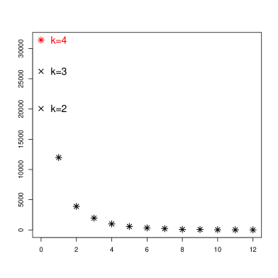
Figure 4: For each data set, graphics of the observed frequencies on the interval [1, 20]. For each $2\leqslant k\leqslant\widehat{k}$, estimated value of the number of missing classes or species.

For the first example we choose $\widehat{k}=4$ using P1 and $\widehat{k}=5$ using P2, while for the two last data sets, we choose $\widehat{k}=k_{\max}$. This choice may be explained by the followed shape of the empirical distributions together with the difficulty of rejecting $H^{k}$ for large $k$.

The number of Shakespeare’s unused words was estimated to be at least equal to 35000 by [16]. Using our procedure with $k_{\max}=6$, we get approximatively 50000 words. In that example $D$ is large enough to protect us against lack of power for testing $H^{k}$, at least for $k\leqslant 4$. Therefore we are confident that $k=6$ is a reasonable choice.

Concerning the number of strains, the estimation given by the Chao1 procedure [11], $\widehat{N}=D+f_{1}^{2}/2f_{2}$, equals 9940, while the estimation given by [26] is 25700 with a $95\%$ confidence interval equals to $[19421,36355]$. Choosing $k=6$ we get $\widehat{N}=13207$. Let us see (Table 17) what happens if $k$ increases: for any $7\leqslant k\leqslant 13$ the hypothesis $H^{k}$ is not rejected. If $k=12$ we get $\widehat{N}=23561$ which is close to the value proposed by Li-Thiao-Té et al. [26]. Nevertheless, the estimated standard-error $\widehat{s}^{k}$ increases drastically with $k$, making the result useless for large $k$.

Number of microbial strains in the human gut microbiome : $D=3180$ strains seen

	$k=7$	$k=8$	$k=9$	$k=10$	$k=11$	$k=12$	$k=13$
$\widehat{N}^{k}$	14447	15675	16962	18458	20469	23561	28695
$\widehat{s}^{k}$	770	1218	2004	3401	5900	10378	18411

Table 17: Estimation of $N$ and of the standard-error of $\widehat{N}^{k}$, for $7\leqslant k\leqslant 13$.

7 Conclusion

We proposed two testing procedures and their boostrap versions to test the null hypothesis that a discrete distribution is $k$-monotone against that it is not, without any parametric assumption on the true underlying distribution. We state the theoretical asymptotic properties of the procedures and carry out a large simulation study in order to assess their performances for finite sample cases. The simulation shows that the tests may present a power fault and require large values of the sample size $d$, in particular when $k$ is large. We compare this non-parametric setting with a parametric procedure for Poisson distribution, when the problem is to test the null hypothesis that the distribution is at least $k$-monotone against the alternative that it is $(k-1)$-monotone but not $k$-monotone. We conclude that the efficiency (the sample size required for the test to achieve a given power) of the non-parametric procedure is much more affected for large values of $k$ than the parametric procedure is. The comparison with the procedure of [7] based on the $\ell^{2}$ distance between the constraint least-squares estimator and the empirical estimator for testing convexity suggests potential improvements.

From these testing procedures we propose a method to infer the degree of $k$-monotonicity of a discrete distribution, assuming that $k$ is smaller than some $k_{\max}$. To our knowledge this is the first method for estimating the degree of $k$ monotonicity of discrete distribution for which theoretical guaranties are established. A large simulation study shows that the performance of the estimator of $k$ depends strongly on the choice of $k_{\max}$: large values of $k_{\max}$ need large sample sizes.

Finally we apply this work to the estimation of the unknown number of classes in a population. Defining a $k$-monotone abundance distribution, the identifiability of the parameter to estimate is ensured. A simulation study shows that the method can be applied providing that the number of seen classes is large, especially as $k$ increases.

8 Proofs

8.1 Proof of Theorem 1

Let us first remark that for $d$ large enough, $\widehat{\tau}$ is almost surely equal to $\tau$. This result comes from the application of the Borel-Cantelli lemma, by noting that

$$\sum_{d=1}^{\infty}P\left(\widehat{\tau}<\tau\right)=\sum_{d=1}^{\infty}(1-p_{\tau})^{d}<+\infty.$$

In the following we will assume that $d$ is large enough to set $\widehat{\tau}=\tau$.

Procedure P1

Let us begin with the testing procedure based on the statistic $\widehat{\mathcal{T}}^{k}$. Because $p$ is $k$-monotone,

$$P\left(\sqrt{d}\min_{0\leqslant j\leqslant\tau-1}\nabla^{k}f_{j}\leqslant q\right) \leqslant P\left(\sqrt{d}\min_{0\leqslant j\leqslant\tau-1}\left(\nabla^{k}f_{j}-\nabla^{k}p_{j}\right)\leqslant q\right)$$

By the central limit theorem we know that the vector $\sqrt{d}A(f-p)$ converges in distribution to a centered Gaussian vector with covariance matrix $A\Gamma A^{T}$, where $\Gamma$ is the matrix with components $\Gamma_{jj^{\prime}}=-p_{j}p_{j^{\prime}}$ if $j\neq j^{\prime}$ and $\Gamma_{jj}=p_{j}(1-p_{j})$ for $0\leqslant j\leqslant\tau-1$. Let $M$ be defined as the square-root of the matrix $A\Gamma A^{T}$, then

$$P\left(\sqrt{d}\min_{0\leqslant j\leqslant\tau-1}\left(\nabla^{k}f_{j}-\nabla^{k}p_{j}\right)\leqslant q\right) = P\left(\sqrt{d}\min_{0\leqslant j\leqslant\tau-1}\sum_{j^{\prime}=0}^{\tau}A_{jj^{\prime}}(f_{j^{\prime}}-p_{j^{\prime}})\leqslant q\right)$$

$$= P\left(\min_{0\leqslant j\leqslant\tau-1}\sum_{j^{\prime}=0}^{\tau-1}M_{jj^{\prime}}\mathcal{Z}_{j^{\prime}}\leqslant q\right)+o(1).$$

uniformly for all $q\in\mathbb{R}$, where the $\mathcal{Z}_{j^{\prime}},j^{\prime}=0,\ldots\tau-1$ are independent centered Gaussian variates.

Because $\widehat{\Gamma}$ converges in probability to $\Gamma$ when $d$ tends to infinity, and thanks to the continuity of the limiting distribution of $\sqrt{d}\min_{j}\left(\nabla^{k}f_{j}-\nabla^{k}p_{j}^{+}\right)$, we get that

$$P\left(\min_{0\leqslant j\leqslant\tau-1}\sum_{j^{\prime}=0}^{\tau-1}M_{jj^{\prime}}\mathcal{Z}_{j^{\prime}}\leqslant\widehat{q}^{k}_{\alpha}\right)=P\left(\min_{0\leqslant j\leqslant\tau-1}\sum_{j^{\prime}=0}^{\tau-1}\widehat{M}_{jj^{\prime}}\mathcal{Z}_{j^{\prime}}\leqslant\widehat{q}^{k}_{\alpha}\right)+o(1)=\alpha+o(1).$$

Let us consider now the case where $p$ is strictly $k$-monotone and let $C\geqslant 0$ be such that $\min_{0\leqslant j\leqslant\tau-1}\nabla^{k}p_{j}\geqslant C$.

$$P\left(\sqrt{d}\min_{0\leqslant j\leqslant\tau-1}\nabla^{k}f_{j}\leqslant q\right) = P\left(\sqrt{d}\min_{0\leqslant j\leqslant\tau-1}\left(\nabla^{k}f_{j}-\nabla^{k}p_{j}\right)\leqslant q-\sqrt{d}C\right)$$

$$= P\left(\min_{0\leqslant j\leqslant\tau-1}\sum_{j^{\prime}=0}^{\tau-1}M_{jj^{\prime}}\mathcal{Z}_{j^{\prime}}\leqslant q-\sqrt{d}C\right)+o(1).$$

Let $q_{\alpha}^{k}$ be defined at Equation (5) and $\sigma^{k}$ be defined in Theorem 1. Applying the Cramer-Chernoff method to Gaussian variables (see for example Massart, 2003, chapter 2), we get the following result:

$$P\left(\min_{0\leqslant j\leqslant\tau-1}\sum_{j^{\prime}=0}^{\tau-1}M_{jj^{\prime}}\mathcal{Z}_{j^{\prime}}\leqslant q^{k}_{\alpha}-\sqrt{d}C\right)\leqslant\tau\exp\left(-\frac{(q^{k}_{\alpha}-\sqrt{d}C)^{2}}{2(\sigma^{k})^{2}}\right).$$ (18)

Then we have:

$$P\left(\min_{0\leqslant j\leqslant\tau-1}\sum_{j^{\prime}=0}^{\tau-1}M_{jj^{\prime}}\mathcal{Z}_{j^{\prime}}\leqslant q^{k}_{\alpha}-\sqrt{d}C\right)\leqslant\tau\exp\left(-\frac{dC^{2}}{2(\sigma^{k})^{2}}\right)\leqslant\beta$$

as soon as $C\geqslant\sqrt{2/d}\sigma^{k}\sqrt{\log((\tau)/\beta)}$.

Procedure P2

Let us now consider the procedure based on $\widehat{\mathcal{S}}_{\alpha}^{k}$. The proof of the first part of the theorem is similar to the proof for the procedure P1. Let us consider the case where $p$ is strictly $k$-monotone. If $\min_{j}\nabla^{k}_{j}\geqslant C$, $\zeta^{k}_{j}=\sqrt{A^{kT}_{j}\Gamma A^{k}_{j}}$ and and $\zeta^{k}=\max_{j}\zeta_{j}^{k}$,

$$\mathbb{P}\left(\widehat{\mathcal{S}}^{k}_{\alpha}\leqslant 0\right) = \mathbb{P}\left(\min_{0\leqslant j\leqslant\tau-1}\left\{\sqrt{d}\nabla^{k}{f}_{j}-\nu_{u^{k}_{\alpha}}\zeta^{k}_{j}\right\}\leqslant 0\right)$$

$$\leqslant \mathbb{P}\left(\min_{0\leqslant j\leqslant\tau-1}\left\{A^{kT}_{j}\Gamma^{1/2}\mathcal{Z}-\nu_{u^{k}_{\alpha}}\zeta^{k}_{j}\right\}\leqslant-\sqrt{d}C\right)+o(1)$$

Then:

$$\mathbb{P}\left(\widehat{\mathcal{S}}^{k}_{\alpha}\leqslant 0\right)\leqslant\tau\max_{j}\;\mathbb{P}\left(A^{kT}_{j}\Gamma^{1/2}\mathcal{Z}\leqslant\nu_{u^{k}_{\alpha}}\zeta^{k}_{j}-\sqrt{d}C\right)+o(1)$$ (19)

Moreover,

$$\mathbb{P}\left(A^{kT}_{j}\Gamma^{1/2}\mathcal{Z}\leqslant\nu_{u^{k}_{\alpha}}\zeta^{k}_{j}-\sqrt{d}C\right)\leqslant\exp\left(-\frac{\left(\nu_{u^{k}_{\alpha}}\zeta^{k}_{j}-\sqrt{d}C\right)^{2}}{2(\zeta^{k}_{j})^{2}}\right).$$

Then we have:

$$\mathbb{P}\left(\widehat{\mathcal{S}}^{k}_{\alpha}\leqslant 0\right)\leqslant\tau\max_{j}\;\exp\left(-\frac{dC^{2}}{2(\zeta^{k}_{j})^{2}}\right)+o(1)\leqslant\beta+o(1)$$

as soon as

$$C\geqslant\frac{1}{\sqrt{d}}\left(\zeta^{k+1}\sqrt{2\log\frac{\tau}{\beta}}\right).$$

8.2 Proof of Theorem 2

Procedure P1

Let $q<0$ and $C$ such that $\nabla^{k+1}p_{j_{0}}\leqslant-C$,

$$\mathbb{P}\left(\widehat{\mathcal{T}}^{k+1}\geqslant q|D=d\right) \leqslant \mathbb{P}\left(\sqrt{d}\nabla^{k+1}f_{j_{0}}\geqslant q\right)$$

$$\leqslant \mathbb{P}\left(\sqrt{d}(\nabla^{k+1}f_{j_{0}}-\nabla^{k+1}p_{j_{0}})\geqslant q-\sqrt{d}\nabla^{k+1}p_{j_{0}}\right)$$

$$\leqslant \mathbb{P}\left(\sqrt{d}(\nabla^{k+1}f_{j_{0}}-\nabla^{k+1}p_{j_{0}})\geqslant q+C\sqrt{d}\right)$$

$$\leqslant \mathbb{P}\left(\sqrt{d}A^{k+1T}_{j_{0}}\mathcal{Z}\geqslant q+C\sqrt{d}\right)+o(1)$$

Applying the classical Tchebychev inequality, we get

$$\mathbb{P}\left(\sqrt{d}A^{k+1T}_{j_{0}}\mathcal{Z}\geqslant q^{k+1}_{\alpha}+C\sqrt{d}\right)\leqslant\exp\left(-\frac{(q^{k+1}_{\alpha}+C\sqrt{d})^{2}}{2(\zeta^{k+1}_{j_{0}})^{2}}\right).$$ (20)

Let us remark that applying Formula (18) to the case where $C=0$, we get

$$\alpha\leqslant\tau\exp\left(-\frac{(q^{k+1}_{\alpha})^{2}}{2(\sigma^{k+1})^{2}}\right)$$

then

$$q_{\alpha}^{k+1}\geqslant-\sigma^{k+1}\sqrt{2\log\frac{\tau}{\alpha}}.$$ (21)

Considering inequalites given at Equations (20) and (21), we get that

$$\mathbb{P}_{\bar{H}^{k+1}(C)}\left(\sqrt{d}A^{k+1T}_{j_{0}}\mathcal{Z}\geqslant q^{k+1}_{\alpha}+C\sqrt{d}\right)\leqslant\beta$$

as soon as

$$C\geqslant\frac{1}{\sqrt{d}}\left(\sigma^{k+1}\sqrt{2\log\frac{\tau}{\alpha}}+\zeta^{k+1}_{j_{0}}\sqrt{-2\log\beta}\right).$$

Procedure P2

Let $C$ be a real such that $\nabla^{k+1}p_{j_{0}}\leqslant-C$, and let $\zeta^{k+1}_{j_{0}}=\sqrt{A^{kT}_{j_{0}}\Gamma A^{k+1}_{j_{0}}}$. We have:

$$\mathbb{P}\left(\widehat{\mathcal{S}}_{\alpha}^{k}\geqslant 0|D=d\right) = \mathbb{P}\left(\min_{0\leqslant j\leqslant\widehat{\tau}-1}\left\{\sqrt{d}\nabla^{k+1}{f}_{j}-\nu_{\widehat{u}^{k+1}_{\alpha}}\sqrt{A^{k+1T}_{j}\widehat{\Gamma}A^{k+1}_{j}}\right\}\geqslant 0\right)$$

$$\leqslant \mathbb{P}\left(\sqrt{d}(\nabla^{k+1}f_{j_{0}}-\nabla^{k+1}p_{j_{0}})\geqslant\nu_{\widehat{u}^{k+1}_{\alpha}}\sqrt{A^{k+1T}_{j_{0}}\widehat{\Gamma}A^{k+1}_{j_{0}}}+C\sqrt{d}\right)$$

$$\leqslant \mathbb{P}\left(\sqrt{d}A^{k+1T}_{j_{0}}\mathcal{Z}\geqslant\nu_{u^{k+1}_{\alpha}}\zeta^{k+1}_{j_{0}}+C\sqrt{d}\right)+o(1)$$

Applying the classical Tchebychev inequality, we get

$$\mathbb{P}\left(\sqrt{d}A^{k+1T}_{j_{0}}\mathcal{Z}\geqslant\nu_{u^{k+1}_{\alpha}}\zeta^{k+1}_{j_{0}}+C\sqrt{d}\right)\leqslant\exp\left(-\frac{(\nu_{u^{k+1}_{\alpha}}\zeta^{k+1}_{j_{0}}+C\sqrt{d})^{2}}{2(\zeta^{k+1}_{j_{0}})^{2}}\right).$$ (22)

Let us remark that applying Formula (19) to the case where $C=0$, we get

$$\alpha\leqslant\tau\max_{j}\;u_{\alpha}^{k}$$

then $u_{\alpha}^{k+1}\geqslant\alpha/\tau$ and

$$\nu_{u_{\alpha}^{k+1}}\geqslant\nu_{\alpha/\tau}\geqslant-\sqrt{2\log\frac{\tau}{\alpha}}.$$ (23)

Considering inequalites given at Equations (22) and (23), we get that

$$\mathbb{P}_{\bar{H}^{k+1}(C)}\left(\sqrt{d}A^{k+1T}_{j_{0}}\mathcal{Z}\geqslant\nu_{u^{k+1}_{\alpha}}\zeta^{k+1}_{j_{0}}+C\sqrt{d}\right)\leqslant\beta$$

as soon as

$$C\geqslant\frac{1}{\sqrt{d}}\left(\sqrt{2\log\frac{\tau}{\alpha}}+\sqrt{-2\log\beta}\right)\zeta^{k+1}_{j_{0}}.$$

8.3 Proof of Theorem 3

If $k=1$,

$$\mathbb{P}\left(\widehat{k}_{\alpha}=0\right) = \mathbb{P}\left(H^{1}\mbox{ is rejected}\right)\leqslant\alpha+o(1)$$

Let us now consider the case where $k\geqslant 2$

$$\mathbb{P}\left(\widehat{k}_{\alpha}\leqslant k-1\right) = \mathbb{P}\left(\exists\ell,1\leqslant\ell\leqslant k-1,\forall m\leqslant\ell,H^{m}\mbox{ is not rejected and }H^{\ell+1}\mbox{ is rejected}\right)$$

$$\leqslant \mathbb{P}\left(\exists\ell,1\leqslant\ell\leqslant k-1,H^{\ell+1}\mbox{ is rejected}\right)$$

$$\leqslant \mathbb{P}\left(H^{k}\mbox{ is rejected}\right)+\mathbb{I}_{\left(k\geqslant 3\right)}\sum_{\ell=1}^{k-2}\mathbb{P}\left(H^{\ell+1}\mbox{ is rejected}\right)$$

Thanks to Theorem 1, taking $\beta=1/(k-2)\sqrt{d}$ if $k\geqslant 3$, we get the first part of the Theorem.

For the second part of the theorem

$$\mathbb{P}\left(\widehat{k}_{\alpha}\geqslant k+1\right) = \sum_{\ell=k+1}^{k_{\max}}\mathbb{P}\left(\widehat{k}_{\alpha}=\ell\right)$$

$$= \sum_{\ell=k+1}^{k_{\max}}\mathbb{P}\left(\forall m,1\leqslant m\leqslant\ell,H^{m}\mbox{ is not rejected and }H^{\ell+1}\mbox{ is rejected}\right)$$

$$\leqslant \sum_{\ell=k+1}^{k_{\max}}\mathbb{P}\left(\forall m,k+1\leqslant m\leqslant\ell,H^{m}\mbox{ is not rejected }\right)$$

$$\leqslant (k_{\max}-k-1)\mathbb{P}\left(H^{k+1}\mbox{ is not rejected }\right).$$

8.4 Bias and variance

$$\widehat{N}^{k} = D-\sum_{h=1}^{k}(-1)^{h}C_{k}^{h}S_{h}$$

$$= D+S_{0}-\nabla^{k}S_{0}$$

$$\mathbb{E}\left(\widehat{N}^{k}\right) = N-N\nabla^{k}p_{0}$$

Let $\alpha_{k,h}=1-(-1)^{h}C_{k}^{h}$

$$\mathbb{V}\left(\widehat{N}^{k}/\sqrt{N}\right) = \sum_{h=1}^{k}\alpha_{k,h}^{2}p_{h}(1-p_{h})-\sum_{h_{1}\neq h_{2}}\alpha_{k,h_{1}}\alpha_{k,h_{2}}p_{h_{1}}p_{h_{2}}-2\sum_{h=1}^{k}\alpha_{k,h}p_{h}p_{\geqslant k+1}+p_{\geqslant k+1}(1-p_{\geqslant k+1})$$

$$= \sum_{h=1}^{k}\alpha_{k,h}^{2}p_{h}-\sum_{h=1}^{k}\alpha_{k,h}^{2}p_{h}^{2}-\left(\sum_{h=1}^{k}\alpha_{k,h}p_{h}\right)^{2}+\sum_{h=1}^{k}\alpha_{k,h}^{2}p_{h}^{2}$$

$$-2\sum_{h=1}^{k}\alpha_{k,h}p_{h}p_{\geqslant k+1}+p_{\geqslant k+1}-p_{\geqslant k+1}^{2}$$

$$= \sum_{h=1}^{k}\alpha_{k,h}^{2}p_{h}-\left(\sum_{h=1}^{k}\alpha_{k,h}p_{h}+p_{\geqslant k+1}\right)^{2}+p_{\geqslant k+1}$$

$$= \sum_{h=1}^{k}\left(1-(-1)^{h}C_{k}^{h}\right)^{2}p_{h}-\left(\sum_{h=1}^{k}\left(1-(-1)^{h}C_{k}^{h}\right)p_{h}+p_{\geqslant k+1}\right)^{2}+p_{\geqslant k+1}$$

$$= \sum_{h=1}^{k}\left(1-2(-1)^{h}C_{k}^{h}+\left(C_{k}^{h}\right)^{2}\right)p_{h}-\left(\sum_{h=1}^{k}p_{h}+p_{\geqslant k+1}-\sum_{h=1}^{k}(-1)^{h}C_{k}^{h}p_{h}\right)^{2}+p_{\geqslant k+1}$$

$$= 1-p_{0}-2\sum_{h=1}^{k}(-1)^{h}C_{k}^{h}p_{h}+\sum_{h=1}^{k}\left(C_{k}^{h}\right)^{2}p_{h}-\left(1-p_{0}-\sum_{h=1}^{k}(-1)^{h}C_{k}^{h}p_{h}\right)^{2}$$

$$= p_{0}(1-p_{0})-2\sum_{h=1}^{k}(-1)^{h}C_{k}^{h}p_{h}+\sum_{h=1}^{k}\left(C_{k}^{h}\right)^{2}p_{h}+2(1-p_{0})\sum_{h=1}^{k}(-1)^{h}C_{k}^{h}p_{h}$$

$$-\left(\sum_{h=1}^{k}(-1)^{h}C_{k}^{h}p_{h}\right)^{2}$$

$$= p_{0}(1-p_{0})-2p_{0}\sum_{h=1}^{k}(-1)^{h}C_{k}^{h}p_{h}+\sum_{h=1}^{k}\left(C_{k}^{h}\right)^{2}p_{h}-\left(\sum_{h=1}^{k}(-1)^{h}C_{k}^{h}p_{h}\right)^{2}$$

$$= p_{0}-\left(\sum_{h=1}^{k}(-1)^{h}C_{k}^{h}p_{h}+p_{0}\right)^{2}+\sum_{h=1}^{k}\left(C_{k}^{h}\right)^{2}p_{h}$$

$$= p_{0}+\sum_{h=1}^{k}\left(C_{k}^{h}\right)^{2}p_{h}-\left(\nabla^{k}p_{0}\right)^{2}.$$

References

References

- Akakpo et al. [2014] N. Akakpo, F. Balabdaoui, and C. Durot. Testing monotonicity via local least concave majorants. Bernoulli, 20(2):514–544, 2014.
- Balabdaoui and Durot [2015] F. Balabdaoui and C. Durot. Marshall lemma in discrete convex estimation. Statistics & Probability Letters, 99:143–148, 2015.
- Balabdaoui and Jankowski [2016] F. Balabdaoui and H. Jankowski. Maximum likelihood estimation of a unimodal probability mass function. Statistical sinica, 3:1061–1086, 2016.
- Balabdaoui and Wellner [2010] F. Balabdaoui and J. A. Wellner. Estimation of a k-monotone density: characterizations, consistency and minimax lower bounds. Statistica Neerlandica, 64(1):45–70, 2010.
- Balabdaoui et al. [2013] F. Balabdaoui, H. Jankowski, K. Rufibach, and M. Pavlides. Asymptotics of the discrete log-concave maximum likelihood estimator and related applications. Journal of the Royal Statistical Society: Series B (Statistical Methodology), 75(4):769–790, 2013.
- Balabdaoui et al. [2017a] F. Balabdaoui, C. Durot, and F. Koladjo. On asymptotics of the discrete convex lse of a pmf. Bernoulli, 23(3):1449–1480, 2017a.
- Balabdaoui et al. [2017b] F. Balabdaoui, C. Durot, and F. Koladjo. Testing convexity of a discrete distribution. arXiv preprint arXiv:1701.04367, 2017b.
- Böhning et al. [2017] D. Böhning, J. Bunge, and P. Heijden. Capture-recapture Methods for the Social and Medical Sciences. Chapman & Hall/Crc Interdisciplinary Statistics. Taylor & Francis, 2017. ISBN 9781498745314. URL https://books.google.fr/books?id=YGbnAQAACAAJ.
- Böhning Dankmar [2017] v. d. H. P. Böhning Dankmar, Bunge John. Basic concepts of capture-recapture. Chapman and Hall CRC Interdisciplinary Statistics, 2017.
- Bunge and Fitzpatrick [1993] J. Bunge and M. Fitzpatrick. Estimating the number of species: a review. Journal of the American Statistical Association, 88(421):364–373, 1993.
- Chao [1984] A. Chao. Nonparametric estimation of the number of classes in a population. Scandinavian Journal of statistics, pages 265–270, 1984.
- Chee and Wang [2016] C.-S. Chee and Y. Wang. Nonparametric estimation of species richness using discrete k-monotone distributions. Computational Statistics & Data Analysis, 93:107–118, 2016.
- Durot et al. [2013] C. Durot, S. Huet, F. Koladjo, and S. Robin. Least-squares estimation of a convex discrete distribution. Computational Statistics & Data Analysis, 67:282–298, 2013.
- Durot et al. [2015] C. Durot, S. Huet, F. Koladjo, and S. Robin. Nonparametric species richness estimation under convexity constraint. Environmetrics, 26(7):502–513, 2015.
- Durot et al. [2017] C. Durot, J. Giguelay, S. Huet, F. Koladjo, and S. Robin. Convex Estimation. In Capture-Recapture Methods for the Social and Medical Sciences. Chapman and Hall CRC Interdisciplinary Statistics, 2017.
- Efron and Thisted [1976] B. Efron and R. Thisted. Estimating the number of unsen species: How many words did shakespeare know? Biometrika, pages 435–447, 1976.
- Fisher et al. [1943] R. A. Fisher, A. S. Corbet, and C. B. Williams. The relation between the number of species and the number of individuals in a random sample of an animal population. The Journal of Animal Ecology, pages 42–58, 1943.
- Giguelay [2017a] J. Giguelay. Estimation of a discrete probability under constraint of -monotonicity. Electronic Journal of Statistics, 11(1):1–49, 2017a.
- Giguelay [2017b] J. Giguelay. Estimation des moindres carrés d’une densité discrète sous contrainte de k-monotonie et bornes de risque. Application à l’estimation du nombre d’espèces dans une population. PhD thesis, University Paris-Saclay, 2017b.
- Groeneboom and Jongbloed [2014] P. Groeneboom and G. Jongbloed. Nonparametric estimation under shape constraints, volume 38. Cambridge University Press, 2014.
- Groeneboom et al. [2008] P. Groeneboom, G. Jongbloed, and J. A. Wellner. The support reduction algorithm for computing non-parametric function estimates in mixture models. Scandinavian Journal of Statistics, 35(3):385–399, 2008.
- Hser [2001] Y.-I. Hser. Population estimation of illicit drug users in los angeles county. The Journal of Drug Issues, 23:323(334, 2001.
- Jankowski and Wellner [2009] H. K. Jankowski and J. A. Wellner. Estimation of a discrete monotone distribution. Electronic journal of statistics, 3:1567, 2009.
- Kacem et al. [2015] M. Kacem, C. Lefèvre, and S. Loisel. Convex extrema for nonincreasing discrete distributions: Effects of convexity constraints. Journal of Mathematical Analysis and Applications, 423(2):1774 – 1791, 2015. ISSN 0022-247X. doi: http://dx.doi.org/10.1016/j.jmaa.2014.10.071. URL http://www.sciencedirect.com/science/article/pii/S0022247X14010099.
- Lefevre and Loisel [2013] C. Lefevre and S. Loisel. On multiply monotone distributions, continuous or discrete, with applications. Journal of Applied Probability, 50(3):827–847, 2013.
- Li-Thiao-Té et al. [2012] S. Li-Thiao-Té, D. Jean-Jacques, and R. Stéphane. Bayesian model averaging for estimating the number of classes: applications to the total number of species in metagenomics. Journal of Applied Statistics, 39(7):1489–1504, 2012.
- Rao [1969] B. P. Rao. Estimation of a unimodal density. Sankhyā: The Indian Journal of Statistics, Series A, pages 23–36, 1969.
- Reboul [1998] L. Reboul. Estimation sous restriction de forme et application a la fiabilite. Tests de validation d’un modele parametrique pour un processus de poisson non homogene. PhD thesis, Université Paris XI, 1998.
- Reboul [2005] L. Reboul. Estimation of a function under shape restrictions. applications to reliability. Ann. Statist., 33(3):1330–1356, 06 2005. doi: 10.1214/009053605000000138. URL http://dx.doi.org/10.1214/009053605000000138.
- Spevack [1968] M. Spevack. A complete and systematic concordance to the works of shakespeare. vol. 3: Drama and character concordances to the folio tragedies, 1968.
- Tap et al. [2009] J. Tap, S. Mondot, F. Levenez, E. Pelletier, C. Caron, J.-P. Furet, E. Ugarte, R. Muñoz-Tamayo, D. L. Paslier, R. Nalin, et al. Towards the human intestinal microbiota phylogenetic core. Environmental microbiology, 11(10):2574–2584, 2009.