ON THE TIME OF FIRST LEVEL CROSSING AND INVERSE GAUSSIAN DISTRIBUTION

Abstract.

We propose a new approximation for the distribution of the time of the first level $u$ crossing by the random process $V_{s}-cs$, where $V_{s}$, $s>0$, is compound renewal process and $c>0$. It is competitive with respect to existing approximations, particularly in the region around the critical point $c=c^{*}$ which separates processes with positive and negative drifts. This approximation is tightly related to inverse Gaussian distributions.

1. Introduction and main result

The inverse Gaussian distribution has probability density function (p.d.f.)

$$f\left(x;\mu,\lambda,-\tfrac{1}{2}\right)=\frac{\lambda^{1/2}}{\sqrt{2\pi}}\,x^{-3/2}\exp\left\{-\frac{\lambda(x-\mu)^{2}}{2\mu^{2}x}\right\},$$ (1.1)

where $x$, $\mu$, and $\lambda$ are positive. Parameter $\lambda$ is called shape parameter, and $\mu$ is called mean parameter.

In the study of this distribution, paramount is finding explicit expression

$$F\left(x;\mu,\lambda,-\tfrac{1}{2}\right)=\int_{0}^{x}f\left(z;\mu,\lambda,-\tfrac{1}{2}\right)dz\\ =\varPhi_{\left({0},{1}\right)}\left(\sqrt{\frac{\lambda}{x}}\left(\frac{x}{\mu}-1\right)\right)+\exp\bigg{\{}\frac{2\lambda}{\mu}\bigg{\}}\,\varPhi_{\left({0},{1}\right)}\left(-\sqrt{\frac{\lambda}{x}}\left(\frac{x}{\mu}+1\right)\right)$$ (1.2)

for cumulative distribution function (c.d.f.) corresponding to p.d.f. (1.1); by $\varPhi_{\left({0},{1}\right)}(x)$ and $\varphi_{\left({0},{1}\right)}(x)$ we denote c.d.f. and p.d.f. of a standard normal distribution.

By $f_{T_{1}}(t)$ and $f_{T}(t)$ we denote p.d.f. of positive random variable $T_{1}$, and of positive random variables $T_{i}\overset{d}{=}T$, $i=2,3,\dots$, all distributed identically. The random variable $T_{1}$ is the time between starting time zero and time of the first renewal, and the random variables $T_{i}$ are inter-renewal times. By $f_{Y}(t)$ we denote p.d.f. of positive random variables $Y_{i}\overset{d}{=}Y$, $i=1,2,\dots$, all distributed identically. The random variables $Y_{i}$ are called jump sizes, and the jumps occur only in the moments of renewals. Throughout the entire presentation, p.d.f. $f_{T}(y)$ and $f_{Y}(y)$ are assumed bounded from above by a finite constant. Having assumed that $T_{1}$, i.i.d. $T_{i}\overset{d}{=}T$, $i=2,3,\dots$, i.i.d. $Y_{i}\overset{d}{=}Y$, $i=1,2,\dots$, are all mutually independent, we are within renewal model, where the distribution of the first interval $T_{1}$ may be different from the distribution of the other interclaim intervals, i.e., from the distribution of $T$.

Compound renewal process with time $s\geqslant 0$ is

$$V_{s}=\sum_{i=1}^{N_{s}}Y_{i},$$

or $0$, if $N_{s}=0$ (or $T_{1}>s$), where $N_{s}=\max\left\{n>0:\sum_{i=1}^{n}T_{i}\leqslant s\right\}$, or $0$, if $T_{1}>s$. The random variable

$$\Upsilon=\inf\left\{s>0:V_{s}-cs>u\right\},$$ (1.3)

or $+\infty$, as $V_{s}-cs\leqslant u$ for all $s>0$, is the time of the first level $u$ crossing by the process $V_{s}-cs$.

It is easily seen that for $t>0$

$$\mathsf{P}\{\Upsilon\leqslant t\}=\int_{0}^{t}\mathsf{P}\{u+cv-Y_{1}<0\}f_{T_{1}}(v)dv+\int_{0}^{t}\mathsf{P}\{v<\Upsilon\leqslant t\mid T_{1}=v\}f_{T_{1}}(v)dv.$$ (1.4)

This distribution of $\Upsilon$ appears in many branches of applied probability, including risk and queueing theories, and was considered by many authors. For it, there are many closed-form formulas and approximations, derived by different techniques. The goal of this paper is to get the approximation that involves inverse Gaussian distribution, and seems new. Remarkable is that it is derived under a set of conditions similar to those usually imposed in the common local central limit theorem.

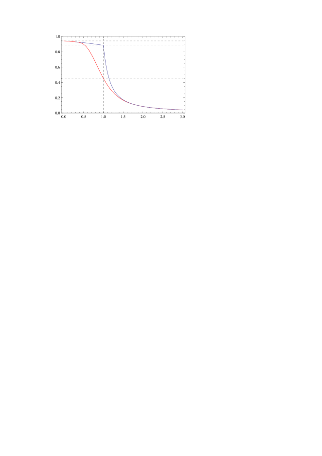
Figure 1. Graphs ($X$-axis is $c$) of the functions ${\mathcal{M}}_{\infty}(u,c,0)$ and ${\mathcal{M}}_{t}(u,c,0)$, as $M=1$, $D^{2}=6$, $t=100$, $u=15$. Horizontal lines are ${\mathcal{M}}_{\infty}(u,0,0)=0.943$, ${\mathcal{M}}_{\infty}(u,c^{*},0)=0.886$, and ${\mathcal{M}}_{t}(u,c^{*},0)=0.454$, where $c^{*}=\mathsf{E}{Y}/\mathsf{E}{T}$.

Set $M={\mathsf{E}{T}}/{\mathsf{E}{Y}}$, $D^{2}=((\mathsf{E}{T})^{2}\mathsf{D}{Y}+(\mathsf{E}{Y})^{2}\mathsf{D}{T})/(\mathsf{E}{Y})^{3}$, and introduce

$${\mathcal{M}}_{t}(u,c,v)=\int_{0}^{\frac{c(t-v)}{u+cv}}\frac{1}{1+x}\,\varphi_{\left({cM(1+x)},{\frac{c^{2}D^{2}(1+x)}{u+cv}}\right)}(x)dx.$$

For $c^{*}=\frac{1}{M}$, $\lambda=\frac{u+cv}{c^{2}D^{2}}>0$, $\mu=\frac{1}{1-cM}$, and $\hat{\mu}=-\mu=\frac{1}{cM-1}$, using (1.1) and (1.2), we have

$${\mathcal{M}}_{t}(u,c,v) =\begin{cases}F\big{(}x;\mu,\lambda,-\tfrac{1}{2}\big{)}\Big{|}_{x=1}^{\frac{c(t-v)}{u+cv}+1},&0<c\leqslant c^{*},\\[6.0pt] \exp\big{\{}-2\,\tfrac{\lambda}{\hat{\mu}}\big{\}}F\big{(}x;\hat{\mu},\lambda,-\tfrac{1}{2}\big{)}\Big{|}_{x=1}^{\frac{c(t-v)}{u+cv}+1},&c\geqslant c^{*}\end{cases}$$

$$=\bigg{[}\varPhi_{\left({0},{1}\right)}\Big{(}\tfrac{\sqrt{u+cv}}{cD\sqrt{x}}\big{(}x(1-cM)-1\big{)}\Big{)}$$

$$\hskip 28.0pt+\exp\Big{\{}2\frac{u+cv}{c^{2}D^{2}}(1-cM)\Big{\}}\varPhi_{\left({0},{1}\right)}\Big{(}-\tfrac{\sqrt{u+cv}}{cD\sqrt{x}}\big{(}x(1-cM)+1\big{)}\Big{)}\bigg{]}\bigg{|}_{x=1}^{\frac{c(t-v)}{u+cv}+1}.$$

Theorem 1.1.

In the above model, let p.d.f. $f_{T}(y)$ and $f_{Y}(y)$ be bounded from above by a finite constant, $D^{2}>0$, $\mathsf{E}({T}^{3})<\infty$, $\mathsf{E}({Y}^{3})<\infty$. Then for $c>0$, for fixed $0<v<t$ we have

$$\sup_{t>v}\Big{|}\,\mathsf{P}\{v<\Upsilon\leqslant t\mid T_{1}=v\}-{\mathcal{M}}_{t}(u,c,v)\Big{|}=\underline{O}\bigg{(}\frac{\ln(u+cv)}{u+cv}\bigg{)},$$ (1.5)

as $u+cv\to\infty$.

As soon as the distribution of $T_{1}$ is specified, the similar results for $\mathsf{P}\{\Upsilon\leqslant t\}$ are straightforward from Theorem 1.1. In particular, for $T_{1}$ exponential with parameter $\beta$

$$\mathsf{P}\{\Upsilon\leqslant t\}=\beta\int_{0}^{t}\mathsf{P}\{u+cv-Y_{1}<0\}e^{-\beta v}dv+\beta\int_{0}^{t}\mathsf{P}\{v<\Upsilon\leqslant t\mid T_{1}=v\}e^{-\beta v}dv.$$

If $Y$ is exponential with parameter $\alpha$, we have

$$\mathsf{P}\{\Upsilon\leqslant t\}=\beta\int_{0}^{t}e^{-\alpha(u+cv)}e^{-\beta v}dv+\beta\int_{0}^{t}\mathsf{P}\{v<\Upsilon\leqslant t\mid T_{1}=v\}e^{-\beta v}dv\\ =\frac{\beta e^{-\alpha u}}{\beta+c\alpha}\big{(}1-e^{-(\beta+c\alpha)t}\big{)}+\beta\int_{0}^{t}\mathsf{P}\{v<\Upsilon\leqslant t\mid T_{1}=v\}e^{-\beta v}dv.$$

2. Closed-form expression using convolutions

The following result is a modification of a result in [Borovkov Dickson 2008].

Theorem 2.1.

For $M(s)=\inf\{k\geqslant 1:\sum_{i=1}^{k}Y_{i}>s\}-1$, we have

$$\mathsf{P}\{v<\Upsilon\leqslant t\mid T_{1}=v\}=\int_{v}^{t}\dfrac{u+cv}{u+cz}\sum_{n=1}^{\infty}\mathsf{P}\big{\{}M(u+cz)=n\big{\}}f_{T}^{*n}(z-v)dz,$$ (2.1)

and

$$\mathsf{P}\{\Upsilon\leqslant t\}=\int_{0}^{t}\mathsf{P}\{u+cv-Y_{1}<0\}f_{T_{1}}(v)dv\\[0.0pt] +\int_{0}^{t}\left[\int_{v}^{t}\frac{cv+u}{u+cs}\sum_{n=1}^{\infty}\mathsf{P}\big{\{}M(u+cs)=n\big{\}}f_{T}^{*n}(s-v)ds\right]f_{T_{1}}(v)dv.$$ (2.2)

Corollary 2.1 (Theorem 1 in [Borovkov Dickson 2008]).

For $Y$ exponential with parameter $\alpha$, we have

$$\mathsf{P}\{\Upsilon\leqslant t\}=\int_{0}^{t}e^{-\alpha(u+cs)}\left[f_{T_{1}}(s)+\frac{1}{u+cs}\sum_{n=1}^{\infty}\frac{(\alpha(u+cs))^{n}}{n!}\right.\\[0.0pt] \left.\times\int_{0}^{s}(u+cv)f_{T}^{*n}(s-v)f_{T_{1}}(v)dv\right]ds.$$ (2.3)

Proof of Theorem 2.1.

The main idea of this proof is to change jumps direction from “toward the boundary” to “away from the boundary” and then use Kendall’s identity. We set $T_{1}=v$ and write

$$\Upsilon=(\sigma-u)/c,$$ (2.4)

where $\sigma$ is the crossing time of the lower level $-(v+u/c)$ by the process $Z(s)=\sum_{k\leqslant M(s)}T_{k}-s/c$ (here $M(s)=\inf\{k\geqslant 1:\sum_{i=1}^{k}Y_{i}>s\}-1$), which is a skip-free in the negative direction Lévy process.

The Kendall’s identity writes as (see [Borovkov Dickson 2008]):

$$p_{\sigma}(s)=\frac{v+u/c}{s}p_{Z(s)}(-(v+u/c)),$$

where

$$p_{Z(s)}(-(v+u/c))=\sum_{n=1}^{\infty}\mathsf{P}\big{\{}M(s)=n\big{\}}f_{T}^{*n}(-(v+u/c)+s/c).$$

According to (2.4), we have $p_{\Upsilon}(t\mid v)=cp_{\sigma}(u+ct)$. We observe that $\Upsilon\geqslant T_{1}$ holds always and write

$$\mathsf{P}\{\Upsilon\leqslant t\}=\mathsf{P}\{T_{1}=\Upsilon\leqslant t\}+\mathsf{P}\{T_{1}<\Upsilon\leqslant t\}\\ =\int_{0}^{t}\mathsf{P}\{u+cv-Y_{1}<0\}f_{T_{1}}(v)dv+\int_{0}^{t}\mathsf{P}\{v<\Upsilon\leqslant t\mid T_{1}=v\}f_{T_{1}}(v)dv\\ =\int_{0}^{t}\mathsf{P}\{u+cv-Y_{1}<0\}f_{T_{1}}(v)dv+\int_{0}^{t}\left[\int_{v}^{t}p_{\Upsilon}(z\mid v)dz\right]f_{T_{1}}(v)dv\\ =\int_{0}^{t}\mathsf{P}\{u+cv-Y_{1}<0\}f_{T_{1}}(v)dv+\int_{0}^{t}\left[\int_{v}^{t}cp_{\sigma}(u+cs)ds\right]f_{T_{1}}(v)dv$$

with

$$cp_{\sigma}(u+cs)=\frac{cv+u}{u+cs}\sum_{n=1}^{\infty}\mathsf{P}\big{\{}M(u+cs)=n\big{\}}f_{T}^{*n}(s-v),$$

which is required. ∎

Proof of Corollary 2.1.

For $Y_{i}\overset{d}{=}Y$, $i=1,2,\dots$, exponential with parameter $\alpha$, we have

$$\mathsf{P}\big{\{}M(u+cs)=n\big{\}}=e^{-\alpha(u+cs)}\frac{(\alpha(u+cs))^{n}}{n!},\quad n=1,2,\dots,$$

$\mathsf{P}\{u+cv-Y_{1}<0\}=e^{-\alpha(u+cv)}$, and equation (2.2) turns into (2.3), as required. ∎

3. Proof of Theorem 1.1

In the sequel, let $K$, $K_{1}$, $K_{2}$, etc., be “sufficiently large” positive constants, and $\epsilon$, $\epsilon_{1}$, $\epsilon_{2}$, etc., be “sufficiently small” positive constants. All of them do not depend on summation and integration variables, such as $n$, $y$, $z$, etc., and possibly are different in different equations.

We put $y=z-v$ in (2.1) and rewrite it as

$$\mathsf{P}\{v<\Upsilon\leqslant t\mid T_{1}=v\} =\int_{0}^{t-v}\dfrac{u+cv}{u+cv+cy}\,\,\mathsf{p}_{\big{\{}\sum_{i=2}^{M(u+cv+cy)+1}T_{i}\big{\}}}(y)dy$$

$$=\sum_{n=1}^{\infty}\int_{0}^{t-v}\frac{u+cv}{u+cv+cy}\int_{0}^{u+cv+cy}\mathsf{P}\left\{Y_{n+1}>z\right\}$$

$$\hskip 90.0pt\times f_{Y}^{*n}(u+cv+cy-z)f_{T}^{*n}(y)dydz.$$ (3.1)

Bearing in mind that $T_{i}$, $i=1,2,\dots$ and $Y_{i}$, $i=1,2,\dots$ are mutually independent, the second equality in (3.1) holds true since

$$\mathsf{P}\{M(u+cv+cy)=n\}=\mathsf{P}\bigg{\{}\sum_{i=1}^{n}Y_{i}\leqslant u+cv+cy<\sum_{i=1}^{n+1}Y_{i}\bigg{\}}\\ =\int_{0}^{u+cv+cy}f^{*n}_{Y}(u+cv+cy-z)\mathsf{P}\{Y_{n+1}>z\}dz.$$

The proof of Theorem 1.1 consists of several steps. The first and the third steps are elimination of the terms that have little impact in (3.1); it may be called preparation of (3.1) for further analysis. The former is elimination of those terms that correspond to small $n$, i.e., to such $n$ that the event $\{M(u+cv+cy)=n\}$ has a small probability, provided that $u+cv+cy$ is large. The latter is elimination of the terms containing $z$, i.e., defect of the random walk $\sum_{i=1}^{n}Y_{i}$, $n=1,2,\dots$, as it nearly crosses the high level $u+cv+cy$. In the first step, we use the bounds for large deviations of sums of i.i.d. random variables, like in [Nagaev 1965]. In the third step, we apply the Taylor formula to the normal p.d.f.

The second step yields the main term of approximation and the corresponding remainder term in a raw form. That is made by means of applying standard non-uniform Berry-Esseen bounds in local CLT formulated in Section 4.1 to the product of $f^{*n}_{Y}$ and $f^{*n}_{T}$ in (3.1). The fourth step consists in investigation of the asymptotic behavior of core components in the remainder terms which appear all over the proof. The fifth step is the simplification of the main term of approximation, up to the terms of required order of magnitude. It relies on a standard estimation technique developed on the fourth step.

3.1. Step 1: reducing of the area of summation

Let us rewrite (3.1) as

$$\mathsf{P}\{v<\Upsilon\leqslant t\mid T_{1}=v\} =\int_{0}^{t-v}\dfrac{u+cv}{u+cv+cy}\,\,\mathsf{p}_{\big{\{}\sum_{i=2}^{M(u+cv+cy)+1}T_{i}\big{\}}}(y)dy$$

$$=\sum_{n=1}^{\infty}\int_{0}^{t-v}\dfrac{u+cv}{u+cv+cy}\,\,\mathsf{P}\{M(u+cv+cy)=n\}\,\mathsf{p}_{\big{\{}\sum_{i=2}^{n+1}T_{i}\big{\}}}(y)dy,$$

select $N_{\epsilon}=\epsilon\,(u+cv)$, where $0<\epsilon<1$, split the sum $\sum_{1}^{\infty}=\sum_{1}^{N_{\epsilon}}+\sum_{N_{\epsilon}}^{\infty}$ and show that the first summand may be omitted within the required accuracy of approximation.

Note that $(u+cv)/(u+cv+cy)<1$ for $y>0$. Since

$$\mathsf{P}\{M(u+cv+cy)=n\}=\mathsf{P}\bigg{\{}\sum_{i=1}^{n}Y_{i}\leqslant u+cv+cy<\sum_{i=1}^{n+1}Y_{i}\bigg{\}}\leqslant\mathsf{P}\bigg{\{}\sum_{i=1}^{n+1}Y_{i}>u+cv+cy\bigg{\}},$$

we have

$$\sum_{n=1}^{N_{\epsilon}}\int_{0}^{t-v}\mathsf{P}\{M(u+cv+cy)=n\}\mathsf{p}_{\big{\{}\sum_{i=2}^{n+1}T_{i}\big{\}}}(y)dy$$

$$\leqslant\sum_{n=1}^{N_{\epsilon}}\int_{0}^{t-v}\mathsf{P}\bigg{\{}\sum_{i=1}^{n+1}Y_{i}>u+cv+cy\bigg{\}}\mathsf{p}_{\big{\{}\sum_{i=2}^{n+1}T_{i}\big{\}}}(y)dy$$

$$\leqslant\sum_{n=1}^{N_{\epsilon}}\mathsf{P}\bigg{\{}Y_{1}+\sum_{i=2}^{n+1}X_{i}>u+cv\bigg{\}}.$$

For standardized i.i.d. random variables $\tilde{X}_{i}=(X_{i}-\mathsf{E}{X})/\sqrt{\mathsf{D}{X}}$, $i=1,2,\dots$, we have

$$\mathsf{P}\bigg{\{}\sum_{i=2}^{n+1}X_{i}>u+cv\bigg{\}}=\mathsf{P}\bigg{\{}\sum_{i=2}^{n+1}\tilde{X_{i}}>\frac{u+cv-n\mathsf{E}{X}}{\sqrt{\mathsf{D}{X}}}\bigg{\}}.$$

It is easily seen that the inequality

$$\frac{u+cv-n\mathsf{E}{X}}{\sqrt{\mathsf{D}{X}}}>K\sqrt{n\ln(n)}$$

holds true for all $n\leqslant N_{\epsilon}$, and by Lemma 4.1 we have

$$\mathsf{P}\bigg{\{}\sum_{i=2}^{n+1}\tilde{X_{i}}>\frac{u+cv-n\mathsf{E}{X}}{\sqrt{\mathsf{D}{X}}}\bigg{\}}\leqslant K\frac{n}{(u+cv-n)^{3}}.$$

Using simple estimates, we have

$$\sum_{n=1}^{N_{\epsilon}}\mathsf{P}\bigg{\{}Y_{1}+\sum_{i=2}^{n+1}X_{i}>u+cv\bigg{\}}\leqslant K\,\sum_{n=1}^{N_{\epsilon}}\frac{n}{(u+cv-n)^{3}}=\frac{K}{(u+cv)^{3}}\,\sum_{n=1}^{N_{\epsilon}}\frac{n}{(1-\frac{n}{u+cv})^{3}}\\ \leqslant\frac{K_{1}}{(u+cv)^{3}}\,\sum_{n=1}^{N_{\epsilon}}n=\frac{K_{1}}{(u+cv)^{3}}\,\frac{N_{\epsilon}(N_{\epsilon}+1)}{2}=\underline{O}((u+cv)^{-1}),$$

as $u+cv\to\infty$, as required.

3.2. Step 2: application of CLT

For i.i.d. random vectors $\xi_{i}=(\tilde{Y}_{i},\tilde{T}_{i})\in\mathsf{R}^{2}$ with standardized independent components $\tilde{Y}_{i}=(Y_{i}-\mathsf{E}{Y})/\sqrt{\mathsf{D}{Y}}$ and $\tilde{T}_{i}=(T_{i}-\mathsf{E}{T})/\sqrt{\mathsf{D}{T}}$, $i=1,2,\dots$, let us apply Theorem 4.2. Bearing in mind that

$$f_{T}^{*n}(x)=\frac{1}{\sqrt{n\mathsf{D}{T}}}\,p_{n^{-1/2}\sum_{i=1}^{n}\tilde{T}_{i}}\left(\tfrac{x-n\mathsf{E}{T}}{\sqrt{n\mathsf{D}{T}}}\right),\quad f_{Y}^{*n}(x)=\frac{1}{\sqrt{n\mathsf{D}{Y}}}\,p_{n^{-1/2}\sum_{i=1}^{n}\tilde{Y}_{i}}\left(\tfrac{x-n\mathsf{E}{Y}}{\sqrt{n\mathsf{D}{Y}}}\right),$$

we have from Theorem 4.2

$$\Big{|}\,\mathsf{P}\{v<\Upsilon\leqslant t\mid T_{1}=v\}-\mathcal{A}_{t}(u,c\mid T_{1}=v)\Big{|}\leqslant\mathcal{R}_{t}(u,c\mid T_{1}=v),$$ (3.2)

where $c,u>0$, $0<v<t$ and

$$\mathcal{A}_{t}(u,c\mid T_{1}=v) =\sum_{n=N_{\epsilon}}^{\infty}\int_{0}^{t-v}\frac{u+cv}{u+cv+cy}\int_{0}^{u+cv+cy}\mathsf{P}\left\{Y_{n+1}>z\right\}$$

$$\hskip-40.0pt\times\frac{1}{\sqrt{n\mathsf{D}{Y}}}\,\varphi_{\left({0},{1}\right)}\left(\tfrac{u+cv+cy-z-n\mathsf{E}{Y}}{\sqrt{n\mathsf{D}{Y}}}\right)\frac{1}{\sqrt{n\mathsf{D}{T}}}\,\varphi_{\left({0},{1}\right)}\left(\tfrac{y-n\mathsf{E}{T}}{\sqrt{n\mathsf{D}{T}}}\right)\,dydz,$$

$$\mathcal{R}_{t}(u,c\mid T_{1}=v) =K\sum_{n=N_{\epsilon}}^{\infty}\int_{0}^{t-v}\frac{u+cv}{u+cv+cy}\int_{0}^{u+cv+cy}\mathsf{P}\left\{Y_{n+1}>z\right\}$$

$$\hskip-40.0pt\times\frac{1}{n^{3/2}}\bigg{(}1+\bigg{[}\bigg{(}\frac{u+cv+cy-z-n\mathsf{E}{Y}}{\sqrt{n\mathsf{D}{Y}}}\bigg{)}^{2}+\bigg{(}\frac{y-n\mathsf{E}{T}}{\sqrt{n\mathsf{D}{T}}}\bigg{)}^{2}\bigg{]}^{1/2}\bigg{)}^{-3}\,dydz.$$

Remark 3.1.

To get the approximation (3.2), to the product $f_{Y}^{*n}(u+cv+cy-z)f_{T}^{*n}(y)$ we applied Theorem 4.2, which is the Berry-Esseen bounds in two-dimensional local CLT. Instead, we could apply the Berry-Esseen bounds in one-dimensional local CLT to each of these factors, separately. We preferred to use Theorem 4.2 to get the remainder term $\mathcal{R}_{t}(u,c\mid T_{1}=v)$ in a form better suited for the further analysis.

3.3. Step 3: bringing the approximation to a convenient form

We do this in several steps. Major objective is simplification of the main term $\mathcal{A}_{t}(u,c\mid T_{1}=v)$ and verification that the remainder term $\mathcal{R}_{t}(u,c\mid T_{1}=v)$ is of required order of smallness.

Change of variables

Put $x=c\,y/(u+cv)$, $dx=c\,dy/(u+cv)$. For

$$\mathcal{Y}_{n,z}(u+cv,x)=\dfrac{(u+cv)(1+x)-z-n\mathsf{E}{Y}}{\sqrt{n\mathsf{D}{Y}}},\hskip 6.0pt\mathcal{T}_{n}(u+cv,x)=\dfrac{(u+cv)x/c-n\mathsf{E}{T}}{\sqrt{n\mathsf{D}{T}}}$$

we have

$$\mathcal{A}_{t}(u,c\mid T_{1}=v)=\frac{u+cv}{c\sqrt{\mathsf{D}{T}\mathsf{D}{Y}}}\,\sum_{n=N_{\epsilon}}^{\infty}n^{-1}\,\int_{0}^{\frac{c(t-v)}{u+cv}}\frac{1}{1+x}\int_{0}^{(u+cv)(1+x)}\mathsf{P}\left\{Y>z\right\}\\ \times\varphi_{\left({0},{1}\right)}\big{(}\mathcal{Y}_{n,z}(u+cv,x)\big{)}\,\varphi_{\left({0},{1}\right)}\big{(}\mathcal{T}_{n}(u+cv,x)\big{)}\,dxdz$$ (3.3)

and

$$\mathcal{R}_{t}(u,c\mid T_{1}=v)=K(u+cv)\sum_{n=N_{\epsilon}}^{\infty}n^{-3/2}\int_{0}^{\frac{c(t-v)}{u+cv}}\frac{1}{1+x}\int_{0}^{(u+cv)(1+x)}\mathsf{P}\left\{Y>z\right\}\,\\ \times\big{(}1+\big{[}\mathcal{Y}^{2}_{n,z}(u+cv,x)+\mathcal{T}^{2}_{n}(u+cv,x)\big{]}^{1/2}\big{)}^{-3}\,dxdz.$$ (3.4)

Use of fundamental identities of Section 4.3

Denoting

$$B_{1}=(\mathsf{E}{T})^{2}\mathsf{D}{Y}+(\mathsf{E}{Y})^{2}\mathsf{D}{T},\ B_{2}=\mathsf{E}{Y}\mathsf{D}{T},\ B_{3}=\mathsf{E}{T}\mathsf{D}{Y},\ B_{4}=\mathsf{D}{Y}\mathsf{D}{T},$$

we set

$$\begin{gathered}\Delta_{n,z}(u+cv,x)=\dfrac{(u+cv)(x/c)\mathsf{E}{Y}-[(u+cv)(1+x)-z]\mathsf{E}{T}}{\sqrt{B_{1}n}},\\ \Lambda_{n,z}(u+cv,x)=\dfrac{B_{1}n-\big{(}B_{2}[(u+cv)(1+x)-z]+B_{3}(u+cv)x/c\big{)}}{\sqrt{B_{1}B_{4}n}}.\end{gathered}$$ (3.5)

By Lemma 4.2, we have the identity

$$\mathcal{Y}^{2}_{n,z}(u+cv,x)+\mathcal{T}^{2}_{n}(u+cv,x)=\Lambda_{n,z}^{2}(u+cv,x)+\Delta^{2}_{n,z}(u+cv,x),$$

and equation (3.3) rewrites as

$$\mathcal{A}_{t}(u,c\mid T_{1}=v)=\frac{u+cv}{2\pi c\sqrt{\mathsf{D}{T}\mathsf{D}{Y}}}\sum_{n=N_{\epsilon}}^{\infty}n^{-1}\int_{0}^{\frac{c(t-v)}{u+cv}}\frac{1}{1+x}\int_{0}^{(u+cv)(1+x)}\mathsf{P}\left\{Y>z\right\}\\ \times\exp\big{\{}-\tfrac{1}{2}\big{[}\Lambda_{n,z}^{2}(u+cv,x)+\Delta^{2}_{n,z}(u+cv,x)\big{]}\big{\}}dxdz.$$ (3.6)

Equation (3.4) rewrites as

$$\mathcal{R}_{t}(u,c\mid T_{1}=v)=K(u+cv)\sum_{n=N_{\epsilon}}^{\infty}n^{-3/2}\int_{0}^{\frac{c(t-v)}{u+cv}}\frac{1}{1+x}\int_{0}^{(u+cv)(1+x)}\mathsf{P}\left\{Y>z\right\}\,\\ \times\big{(}1+\big{[}\Lambda_{n,z}^{2}(u+cv,x)+\Delta^{2}_{n,z}(u+cv,x)\big{]}^{1/2}\big{)}^{-3}dxdz.$$ (3.7)

Elimination of terms with $z$ in (3.6)

Written in terms of elementary functions and considered as functions of $z$, the expressions (3.6) and (3.7) are liable to such standard calculus manipulations as, e.g., use of Taylor’s formula.

Let us write

$$\mathcal{A}^{\langle 1\rangle}_{t}(u,c\mid T_{1}=v)=\frac{\mathsf{E}{Y}(u+cv)}{2\pi c\sqrt{\mathsf{D}{T}\mathsf{D}{Y}}}\sum_{n=N_{\epsilon}}^{\infty}n^{-1}\int_{0}^{\frac{c(t-v)}{u+cv}}\frac{1}{1+x}\\ \times\exp\big{\{}-\tfrac{1}{2}\big{[}\Lambda^{2}_{n}(u+cv,x)+\Delta_{n}^{2}(u+cv,x)\big{]}\big{\}}dx,$$ (3.8)

where (see (3.5))

$$\Lambda_{n}(u+cv,x)=\Lambda_{n,0}(u+cv,x),\quad\Delta_{n}(u+cv,x)=\Delta_{n,0}(u+cv,x).$$ (3.9)

We need to show that

$$\sup_{t>0}\,\Big{|}\,\mathcal{A}_{t}(u,c\mid T_{1}=v)-\mathcal{A}^{\langle 1\rangle}_{t}(u,c\mid T_{1}=v)\,\Big{|}=\underline{O}\bigg{(}\frac{\ln(u+cv)}{u+cv}\bigg{)},$$

as $u+cv\to\infty$.

Writing $f(z)=\exp\big{\{}-\tfrac{1}{2}\big{[}\Delta^{2}_{n,z}(u+cv,x)+\Lambda_{n,z}^{2}(u+cv,x)\big{]}\big{\}}>0$ and bearing in mind that $\int_{0}^{\infty}\mathsf{P}\left\{Y>z\right\}dz=\mathsf{E}{Y}$, we divide the region of integration with respect to $z$ in (3.6) in two parts, $[0,U_{\epsilon,x}]$ and $[U_{\epsilon,x},(u+cv)(1+x)]$, where $U_{\epsilon,x}=\epsilon(u+cv)(1+x)$, $0<\epsilon<1$.

Bearing in mind that for $z\in[U_{\epsilon,x},(u+cv)(1+x)]$

$$\sup_{z>0}\exp\big{\{}-\tfrac{1}{2}\big{[}\Lambda_{n,z}^{2}(u+cv,x)+\Delta^{2}_{n,z}(u+cv,x)\big{]}\big{\}}=\exp\big{\{}-\tfrac{1}{2}\mathcal{T}^{2}_{n}(u+cv,x)\big{\}}\\[4.0pt] \times\sup_{z>0}\exp\big{\{}-\tfrac{1}{2}\mathcal{Y}^{2}_{n,z}(u+cv,x)\big{\}}\leqslant K\exp\big{\{}-\tfrac{1}{2}\mathcal{T}^{2}_{n}(u+cv,x)\big{\}}$$

and using Chebyshev’s inequality $\mathsf{P}\left\{Y>z\right\}\leqslant\mathsf{E}{Y^{3}}/z^{3}$ which yields

$$\int_{U_{\epsilon,x}}^{(u+cv)(1+x)}\mathsf{P}\left\{Y>z\right\}dz\leqslant\mathsf{E}{Y^{3}}\int_{U_{\epsilon,x}}^{(u+cv)(1+x)}\frac{dz}{z^{3}}\leqslant\frac{K}{(u+cv)^{2}(1+x)^{2}},$$

we have

$$\frac{u+cv}{2\pi c\sqrt{\mathsf{D}{T}\mathsf{D}{Y}}}\sum_{n=N_{\epsilon}}^{\infty}n^{-1}\int_{0}^{\frac{c(t-v)}{u+cv}}\frac{1}{1+x}\int_{U_{\epsilon,x}}^{(u+cv)(1+x)}\mathsf{P}\left\{Y>z\right\}\\[4.0pt] \times\exp\big{\{}-\tfrac{1}{2}\big{[}\Lambda_{n,z}^{2}(u+cv,x)+\Delta^{2}_{n,z}(u+cv,x)\big{]}\big{\}}dxdz\\[4.0pt] \leqslant\frac{K}{u+cv}\int_{0}^{\frac{c(t-v)}{u+cv}}\frac{1}{(1+x)^{3}}\sum_{n=N_{\epsilon}}^{\infty}n^{-1}\exp\big{\{}-\tfrac{1}{2}\mathcal{T}^{2}_{n}(u+cv,x)\big{\}}dx=\underline{O}((u+cv)^{-1}),$$

as $u+cv\to\infty$, which is checked by easy calculus.

For $z\in[0,U_{\epsilon,x}]$, bearing in mind that $\int_{0}^{U_{\epsilon,x}}z\mathsf{P}\left\{Y>z\right\}dz\leqslant\mathsf{E}{Y^{2}}/2<\infty$ and using Taylor’s formula

$$|f(z)-f(0)|\leqslant z\sup_{\xi\in[0,U_{\epsilon,x}]}|f^{\prime}(\xi)|,$$

where $f^{\prime}(z)=f(z)(\mathsf{D}{Y}B_{1}n)^{-1/2}(\mathsf{E}{T}{\sqrt{\mathsf{D}{Y}}}\Delta_{n,z}+\mathsf{E}{Y}\sqrt{\mathsf{D}{T}}\Lambda_{n,z})$, we have to check that

$$\frac{u+cv}{2\pi c\sqrt{\mathsf{D}{T}\mathsf{D}{Y}}}\sum_{n=N_{\epsilon}}^{\infty}n^{-1}(\mathsf{D}{Y}B_{1}n)^{-1/2}\int_{0}^{\frac{c(t-v)}{u+cv}}\frac{1}{1+x}\int_{0}^{U_{\epsilon,x}}z\mathsf{P}\left\{Y>z\right\}dz\\ \times\sup_{\xi\in[0,U_{\epsilon,x}]}\big{(}f(\xi)\,\big{|}\big{(}\mathsf{E}{T}{\sqrt{\mathsf{D}{Y}}}\Delta_{n,\xi}+\mathsf{E}{Y}\sqrt{\mathsf{D}{T}}\Lambda_{n,\xi}\big{)}\big{|}\big{)}dx=\underline{O}\bigg{(}\frac{\ln(u+cv)}{u+cv}\bigg{)},$$

as $u+cv\to\infty$. It follows from

$$(u+cv)\sum_{n=N_{\epsilon}}^{\infty}n^{-3/2}\int_{0}^{\frac{c(t-v)}{u+cv}}\frac{1}{1+x}\sup_{\xi\in[0,U_{\epsilon,x}]}\big{(}f(\xi)\;\big{|}\Lambda_{n,\xi}\big{|}\big{)}\,dx\leqslant K(u+cv)\sum_{n=N_{\epsilon}}^{\infty}n^{-3/2}\\ \times\int_{0}^{\frac{c(t-v)}{u+cv}}\frac{1}{1+x}|\Lambda_{n}|\exp\big{\{}-\tfrac{1}{2}\big{[}\Lambda_{n}^{2}+\Delta^{2}_{n}\big{]}\big{\}}\,dx=\underline{O}\bigg{(}\frac{\ln(u+cv)}{u+cv}\bigg{)}$$ (3.10)

and

$$(u+cv)\sum_{n=N_{\epsilon}}^{\infty}n^{-3/2}\int_{0}^{\frac{c(t-v)}{u+cv}}\frac{1}{1+x}\sup_{\xi\in[0,U_{\epsilon,x}]}\big{(}f(\xi)\;\big{|}\Delta_{n,\xi}\big{|}\big{)}\,dx\leqslant K(u+cv)\sum_{n=N_{\epsilon}}^{\infty}n^{-3/2}\\ \times\int_{0}^{\frac{c(t-v)}{u+cv}}\frac{1}{1+x}|\Delta_{n}|\exp\big{\{}-\tfrac{1}{2}\big{[}\Lambda_{n}^{2}+\Delta^{2}_{n}\big{]}\big{\}}\,dx=\underline{O}\bigg{(}\frac{\ln(u+cv)}{u+cv}\bigg{)},$$ (3.11)

as $u+cv\to\infty$. The proof of (3.10) and (3.11) by means of core asymptotic analysis of the expressions of the second kind is deferred until Step 4.

Elimination of terms with $z$ in (3.4)

Similarly to what just has been done, for

$$\mathcal{R}^{\langle 1\rangle}_{t}(u,c\mid T_{1}=v)=K(u+cv)\sum_{n=N_{\epsilon}}^{\infty}n^{-3/2}\int_{0}^{\frac{c(t-v)}{u+cv}}\frac{1}{1+x}\\ \times\big{(}1+\big{[}\Lambda^{2}_{n}(u+cv,x)+\Delta_{n}^{2}(u+cv,x)\big{]}^{1/2}\big{)}^{-3}dx$$ (3.12)

we need to show that

$$\sup_{t>0}\,\Big{|}\,\mathcal{R}_{t}(u,c\mid T_{1}=v)-\mathcal{R}^{\langle 1\rangle}_{t}(u,c\mid T_{1}=v)\,\Big{|}=\underline{O}\bigg{(}\frac{\ln(u+cv)}{u+cv}\bigg{)},$$ (3.13)

as $u+cv\to\infty$.

We divide as above the region of integration with respect to $z$ in (3.7) in two parts, $[0,U_{\epsilon,x}]$ and $[U_{\epsilon,x},(u+cv)(1+x)]$, where $U_{\epsilon,x}=\epsilon(u+cv)(1+x)$, $0<\epsilon<1$. On the latter, we use Chebyshev’s inequality $\mathsf{P}\left\{Y>z\right\}\leqslant\mathsf{E}{Y^{3}}/z^{3}$. On the former, bearing in mind that $\int_{0}^{U_{\epsilon,x}}z\mathsf{P}\left\{Y>z\right\}dz\leqslant\mathsf{E}{Y^{2}}/2$, we put $g(z)=\big{(}1+\big{[}\Delta^{2}_{n,z}(u+cv,x)+\Lambda_{n,z}^{2}(u+cv,x)\big{]}^{1/2}\big{)}^{-3}$ and use Taylor’s formula

$$\mid g(z)-g(0)\mid\,\leqslant z\sup_{\xi\in[0,U_{\epsilon,x}]}|g^{\prime}(\xi)|,$$

where $g^{\prime}(z)=-\frac{3}{\sqrt{B_{1}n}}\big{(}\mathsf{E}{T}\Delta_{n,z}+\frac{B_{2}}{\sqrt{B_{4}}}\Lambda_{n,z}\big{)}(\Delta^{2}_{n,z}+\Lambda^{2}_{n,z})^{-1/2}g^{4/3}(z)$. The proof reduces to checking that for all $t>0$

$$(u+cv)\sum_{n=N_{\epsilon}}^{\infty}n^{-3/2}\int_{0}^{\frac{c(t-v)}{u+cv}}\frac{1}{1+x}\int_{U_{\epsilon,x}}^{(u+cv)(1+x)}z^{-3}dz\,\big{(}1+\big{[}\mathcal{T}^{2}_{n}(u+cv,x)\big{]}^{1/2}\big{)}^{-3}dx\\ =\underline{O}((u+cv)^{-1})$$ (3.14)

and

$$(u+cv)\sum_{n=N_{\epsilon}}^{\infty}n^{-2}\int_{0}^{\frac{c(t-v)}{u+cv}}\frac{1}{1+x}\big{(}K_{1}|\Lambda_{n}(u+cv,x)|+K_{2}|\Delta_{n}(u+cv,x)|\big{)}\\ \times\big{(}1+\big{[}\Lambda^{2}_{n}(u+cv,x)+\Delta_{n}^{2}(u+cv,x)\big{]}^{1/2}\big{)}^{-3}dx=\underline{O}\bigg{(}\frac{\ln(u+cv)}{u+cv}\bigg{)},$$ (3.15)

as $u+cv\to\infty$. The proof of (3.14) and (3.15) by means of core asymptotic analysis of the expressions of the first kind, is deferred until Step 4.

Estimation of (3.12)

We need to show that

$$\sup_{t>0}\,\mathcal{R}^{\langle 1\rangle}_{t}(u,c\mid T_{1}=v)=\underline{O}\bigg{(}\frac{\ln(u+cv)}{u+cv}\bigg{)},$$ (3.16)

as $u+cv\to\infty$. The proof of (3.16) with $\mathcal{R}^{\langle 1\rangle}_{t}(u,c\mid T_{1}=v)$ written down in (3.12), carried out by means of core asymptotic analysis of the expressions of the first kind, is deferred until Step 4.

3.4. Step 4: core asymptotic analysis

Before we formulate and prove the main results of this section, we examine in more detail $\Lambda_{n}(u+cv,x)$ and $\Delta_{n}(u+cv,x)$ defined in (3.9). From the definition, it follows straightforwardly that

$$\Lambda_{n}(u+cv,x) =\dfrac{B_{1}n-\big{(}B_{2}(u+cv)(1+x)+B_{3}(u+cv)x/c\big{)}}{\sqrt{B_{1}B_{4}n}}$$

$$=\dfrac{B_{1}n+B_{3}(u+cv)/c-(1+x)(u+cv)(B_{2}+B_{3}/c)}{\sqrt{B_{1}B_{4}n}},$$ (3.17)

$$\Delta_{n}(u+cv,x) =\dfrac{((u+cv)x/c)\mathsf{E}{Y}-(u+cv)(1+x)\mathsf{E}{T}}{\sqrt{B_{1}n}}$$

$$=\dfrac{(u+cv)(1+x)(\mathsf{E}{Y}/c-\mathsf{E}{T})-(u+cv)\mathsf{E}{Y}/c}{\sqrt{B_{1}n}},$$ (3.18)

and that for $0<x<\infty$

$$-\infty<\Lambda_{n}(u+cv,x)\leqslant\frac{B_{1}n-(u+cv)B_{2}}{\sqrt{B_{1}B_{4}n}}=\frac{\sqrt{B_{1}}}{\sqrt{B_{4}}}\Big{(}\sqrt{n}-\frac{B_{2}}{B_{1}}\frac{(u+cv)}{\sqrt{n}}\Big{)}.$$

In Lemmas 4.2–4.4, we proved a number of identities for $\Delta_{n}(\mathcal{X},\mathcal{V})$, $\Lambda_{n}(\mathcal{X},\mathcal{V})$ defined in (4.2). In particular, they hold for $\Delta_{n}(u+cv,x)=\Delta_{n}(\mathcal{X},\mathcal{V})\mid_{\mathcal{X}=(u+cv)(1+x),\mathcal{V}=(u+cv)x/c}$ and $\Lambda_{n}(u+cv,x)=\Lambda_{n}(\mathcal{X},\mathcal{V})\mid_{\mathcal{X}=(u+cv)(1+x),\mathcal{V}=(u+cv)x/c}$. Let us establish two more identities for $\Delta_{n}(u+cv,x)$ and $\Lambda_{n}(u+cv,x)$.

Lemma 3.1.

The following identities hold true:

$$\Delta_{n}(u+cv,x)=\frac{\sqrt{B_{4}}(\mathsf{E}{Y}/c-\mathsf{E}{T})}{(B_{2}+B_{3}/c)}\bigg{[}-\Lambda_{n}(u+cv,x)\\ +\frac{\sqrt{B_{1}}}{\sqrt{B_{4}}}\bigg{(}\sqrt{n}+\frac{B_{3}}{B_{1}c}\frac{(u+cv)}{\sqrt{n}}\bigg{)}\bigg{]}-\frac{\mathsf{E}{Y}}{c\sqrt{B_{1}}}\frac{(u+cv)}{\sqrt{n}}$$ (3.19)

and

$$1+x=\frac{\mathsf{E}{Y}\sqrt{B_{1}B_{4}}}{(B_{1}+B_{3}(\mathsf{E}{Y}/c-\mathsf{E}{T}))}\frac{\sqrt{n}}{(u+cv)}\bigg{[}-\Lambda_{n}(u+cv,x)\\ +\frac{\sqrt{B_{1}}}{\sqrt{B_{4}}}\bigg{(}\sqrt{n}+\frac{B_{3}}{B_{1}c}\frac{(u+cv)}{\sqrt{n}}\bigg{)}\bigg{]}.$$ (3.20)

Proof.

From (3.18) and (3.17), we have two expressions for $(1+x)$:

$$1+x =\frac{\sqrt{B_{1}n}\Delta_{n}(u+cv,x)+(u+cv)\mathsf{E}{Y}/c}{(u+cv)(\mathsf{E}{Y}/c-\mathsf{E}{T})},$$ (3.21)

$$1+x =\frac{B_{1}n+B_{3}(u+cv)/c-\sqrt{B_{1}B_{4}n}\Lambda_{n}(u+cv,x)}{(u+cv)(B_{2}+B_{3}/c)}.$$

To get (3.19), we equate the right-hand sides of both equations (3.21) and do straightforward algebraic transformations. To have (3.20), we transform the right-hand side of the second equation (3.21), bearing in mind that $B_{1}=\mathsf{E}{Y}B_{2}+\mathsf{E}{T}B_{3}$ and consequently that $B_{2}+B_{3}/c=(B_{1}+B_{3}(\mathsf{E}{Y}/c-\mathsf{E}{T}))/\mathsf{E}{Y}$. ∎

Asymptotic analysis of the expressions of the first kind

By the expressions of the first kind we call those arising in the analysis of the remainder term in the approximation (3.2). Their integrands contain rational functions modified by a square root. The first expression of this type (cf. (3.12) and (3.16)) is

$$\mathcal{S}=(u+cv)\sum_{n=N_{\epsilon}}^{\infty}n^{-3/2}\int_{0}^{\infty}\frac{1}{1+x}\big{(}1+\big{[}\Lambda^{2}_{n}(u+cv,x)+\Delta_{n}^{2}(u+cv,x)\big{]}^{1/2}\big{)}^{-3}dx.$$

Other expressions of this type are (cf. (3.15))

$$\mathcal{S}^{[1]}=(u+cv)\sum_{n=N_{\epsilon}}^{\infty}n^{-2}\int_{0}^{\infty}\frac{1}{1+x}|\Lambda_{n}(u+cv,x)|(1+\big{[}\Lambda^{2}_{n}(u+cv,x)\\ +\Delta_{n}^{2}(u+cv,x)\big{]}^{1/2}\big{)}^{-3}dx$$

and

$$\mathcal{S}^{[2]}=(u+cv)\sum_{n=N_{\epsilon}}^{\infty}n^{-2}\int_{0}^{\infty}\frac{1}{1+x}|\Delta_{n}(u+cv,x)|(1+\big{[}\Lambda^{2}_{n}(u+cv,x)\\ +\Delta_{n}^{2}(u+cv,x)\big{]}^{1/2})^{-3}dx.$$

Processing of  $\mathcal{S}$

Applying both identities of Lemma 3.1, we rewrite it as

$$\mathcal{S} =\frac{(B_{1}+B_{3}(\mathsf{E}{Y}/c-\mathsf{E}{T}))}{\mathsf{E}{Y}\sqrt{B_{1}B_{4}}}(u+cv)^{2}\sum_{n=N_{\epsilon}}^{\infty}n^{-1}\int_{0}^{\infty}\bigg{\{}-\Lambda_{n}(u+cv,x)$$

$$+\frac{\sqrt{B_{1}}}{\sqrt{B_{4}}}\bigg{(}\sqrt{n}+\frac{B_{3}}{B_{1}c}\frac{(u+cv)}{\sqrt{n}}\bigg{)}\bigg{\}}^{-1}\Bigg{(}1+\bigg{[}\Lambda^{2}_{n}(u+cv,x)+\bigg{\{}\frac{\sqrt{B_{4}}(\mathsf{E}{Y}/c-\mathsf{E}{T})}{B_{2}+B_{3}/c}$$

$$\times\bigg{[}-\Lambda_{n}(u+cv,x)+\frac{\sqrt{B_{1}}}{\sqrt{B_{4}}}\bigg{(}\sqrt{n}+\frac{B_{3}}{B_{1}c}\frac{(u+cv)}{\sqrt{n}}\bigg{)}\bigg{]}-\frac{\mathsf{E}{Y}}{c\sqrt{B_{1}}}\frac{(u+cv)}{\sqrt{n}}\bigg{\}}^{2}\bigg{]}^{1/2}\Bigg{)}^{-3}dx.$$

Making the change of variables $\xi=-\Lambda_{n}(u+cv,x)$ in the integral with respect to $x$ and bearing in mind that

$$dx=\frac{\sqrt{B_{1}B_{4}n}}{(u+cv)(B_{2}+B_{3}/c)}\,d\xi,$$

we get

$$\mathcal{S}=(u+cv)\sum_{n=N_{\epsilon}}^{\infty}n^{-3/2}\int_{L_{u+cv,n}}^{\infty}\big{(}\xi+R_{u+cv,n}\big{)}^{-1}\\[-2.0pt] \times\big{(}1+\big{[}\xi^{2}+\big{(}K_{c}\hskip 0.5pt\,\big{(}\xi+R_{u+cv,n}\big{)}-M_{u+cv,n}\big{)}^{2}\big{]}^{1/2}\big{)}^{-3}\,d\xi,$$ (3.22)

where

$$\begin{gathered}K_{c}\hskip 0.5pt=\dfrac{\mathsf{E}{Y}\sqrt{B_{4}}[\mathsf{E}{Y}-c\mathsf{E}{T}]}{cB_{1}+B_{3}[\mathsf{E}{Y}-c\mathsf{E}{T}]}\,\begin{cases}\,>0,&c<\frac{\mathsf{E}{Y}}{\mathsf{E}{T}},\\[2.0pt] \,=0,&c=\frac{\mathsf{E}{Y}}{\mathsf{E}{T}},\\[2.0pt] \,<0,&c>\frac{\mathsf{E}{Y}}{\mathsf{E}{T}},\end{cases}\quad M_{u+cv,n}=\frac{\mathsf{E}{Y}}{c\sqrt{B_{1}}}\frac{u+cv}{\sqrt{n}}>0,\ \\[8.0pt] L_{u+cv,n}=\frac{\sqrt{B_{1}}}{\sqrt{B_{4}}}\bigg{(}\frac{B_{2}}{B_{1}}\frac{u+cv}{\sqrt{n}}-\sqrt{n}\bigg{)},\quad R_{u+cv,n}=\frac{\sqrt{B_{1}}}{\sqrt{B_{4}}}\bigg{(}\frac{B_{3}}{B_{1}c}\frac{u+cv}{\sqrt{n}}+\sqrt{n}\bigg{)}>0,\end{gathered}$$

and

$$M_{u+cv,n}-K_{c}\hskip 0.5ptR_{u+cv,n}=\frac{\mathsf{E}{Y}\sqrt{B_{1}}}{cB_{1}+B_{3}[\mathsf{E}{Y}-c\mathsf{E}{T}]}\left(\frac{u+cv}{\sqrt{n}}-[\mathsf{E}{Y}-c\mathsf{E}{T}]\sqrt{n}\right).$$

In the sequel, put for brevity $c^{*}=\mathsf{E}{Y}/\mathsf{E}{T}$.

Lemma 3.2.

We have $\mathcal{S}=\underline{O}\bigg{(}\dfrac{\ln(u+cv)}{u+cv}\bigg{)}$, as $u+cv\to\infty$.

First, we prove Lemma 3.2 for $c=c^{*}$, bearing in mind that $K_{c^{*}}=0$. Then we prove it for $c\neq c^{*}$.

Proof of Lemma 3.2 for $c=c^{*}$.

Let us put for brevity $U=u+c^{*}v$ and $\hat{L}=L_{{u+c^{*}}v,n}$, $\hat{R}=R_{{u+c^{*}}v,n}$, $\hat{M}=M_{{u+c^{*}}v,n}$, i.e., for $\mathcal{A}=\frac{\mathsf{E}{T}}{\sqrt{B_{1}}}\frac{\mathsf{E}{T}\sqrt{\mathsf{D}{Y}}}{\mathsf{E}{Y}\sqrt{\mathsf{D}{T}}}>0$, $\mathcal{B}=\frac{\sqrt{B_{1}}}{\sqrt{\mathsf{D}{Y}\mathsf{D}{T}}}>0$, $\mathcal{C}=\frac{\mathsf{E}{T}}{\sqrt{B_{1}}}>0$, we have

$$\begin{gathered}\hat{L}=\frac{\mathcal{C}^{2}}{\mathcal{A}}\frac{U}{\sqrt{n}}-\mathcal{B}\sqrt{n}\,\begin{cases}\,>0,\ n<\frac{B_{2}}{B_{1}}U,\\[6.0pt] \,<0,\ n>\frac{B_{2}}{B_{1}}U,\end{cases}\quad\hat{R}=\mathcal{A}\frac{U}{\sqrt{n}}+\mathcal{B}\sqrt{n}>0,\\[6.0pt] 0<\hat{M}=\mathcal{C}\dfrac{U}{\sqrt{n}}\,\begin{cases}\,>1,\ n<\frac{(\mathsf{E}{T})^{2}}{B_{1}}U^{2},\\[6.0pt] \,<1,\ n>\frac{(\mathsf{E}{T})^{2}}{B_{1}}U^{2},\end{cases}\quad\hat{L}+\hat{R}=\frac{\mathcal{C}^{2}+\mathcal{A}^{2}}{\mathcal{A}}\frac{U}{\sqrt{n}}>0\end{gathered}$$

and  $\hat{\mathcal{S}}=\mathcal{S}\big{|}_{c=c^{*}}$, i.e., $\hat{\mathcal{S}}=U\sum_{n>N_{\epsilon}}n^{-3/2}\int_{\hat{L}}^{\infty}\big{(}\xi+\hat{R}\big{)}^{-1}\big{(}1+\big{[}\xi^{2}+\hat{M}^{2}\big{]}^{1/2}\big{)}^{-3}\,d\xi$.

It is easily seen that

$$\hat{\mathcal{S}}\leqslant K_{1}\mathcal{I}_{\,1}+K_{2}\mathcal{I}_{\,2},$$ (3.23)

where

$$\mathcal{I}_{\,1} =U\sum_{N_{\epsilon}<n<\frac{(\mathsf{E}{T})^{2}}{B_{1}}\,U^{2}}n^{-3/2}\int_{\hat{L}}^{\infty}\big{(}\xi+\hat{R}\big{)}^{-1}\big{(}\xi^{2}+\hat{M}^{2}\big{)}^{-3/2}\,d\xi,$$

$$\mathcal{I}_{\,2} =U\sum_{n>\frac{(\mathsf{E}{T})^{2}}{B_{1}}\,U^{2}}n^{-3/2}\int_{\hat{L}}^{\infty}\big{(}\xi+\hat{R}\big{)}^{-1}\big{(}1+(2\hat{M}|\xi|)^{1/2}\big{)}^{-3}\,d\xi.$$

The essence of (3.23) is the following. For $n$ such that $\hat{M}>1$, we simplify the denominator $(1+[\xi^{2}+\hat{M}^{2}]^{1/2})^{3}$ by switching to $(\xi^{2}+\hat{M}^{2})^{3/2}$. The latter has no singularity since $\hat{M}>1$. For $n$ such that $\hat{M}<1$, we keep $1$ in the denominator and use the inequality between the arithmetic mean and the geometric mean. Both these estimates are such that the integrals in $\mathcal{I}_{\,1}$ and $\mathcal{I}_{\,2}$ may be evaluated explicitly.

Examining $\mathcal{I}_{\,1}$, the explicit expression for the integral $\int_{\hat{L}}^{\infty}(\xi+\hat{R})^{-1}(\xi^{2}+\hat{M}^{2})^{-3/2}\,d\xi$ is found in Lemma 4.5. Using it, the asymptotic behavior of $\mathcal{I}_{\,1}$, as $U\to\infty$, is checked as required in Section 4.6.

Examining $\mathcal{I}_{\,2}$ and bearing in mind that $\hat{L}<0$ for $n>\frac{(\mathsf{E}{T})^{2}}{B_{1}}\,U^{2}$, we split the integrand and make the change of variables as follows:

$$\int_{\hat{L}}^{\infty}\big{(}\xi+\hat{R}\big{)}^{-1}\big{(}1+(2\hat{M}|\xi|)^{1/2}\big{)}^{-3}\,d\xi\\ =\int_{0}^{\infty}\big{(}\xi+\hat{R}\big{)}^{-1}\big{(}1+(2\hat{M}\xi)^{1/2}\big{)}^{-3}\,d\xi+\int_{0}^{-\hat{L}}\big{(}\hat{R}-\xi\big{)}^{-1}\big{(}1+(2\hat{M}\xi)^{1/2}\big{)}^{-3}\,d\xi\\ =\int_{0}^{\infty}\big{(}2\hat{M}\hat{R}+\zeta\big{)}^{-1}\big{(}1+\sqrt{\zeta}\big{)}^{-3}\,d\zeta+\int_{0}^{-\frac{\hat{L}}{2\hat{M}}}\big{(}2\hat{M}\hat{R}-\zeta\big{)}^{-1}\big{(}1+\sqrt{\zeta}\big{)}^{-3}\,d\zeta.$$

The explicit expressions for two latter integrals are found in Lemma 4.7. Using this result, the asymptotic behavior of $\mathcal{I}_{\,2}$, as $U\to\infty$, is checked as required in Section 4.7. The proof is complete. ∎

Proof of Lemma 3.2 for $c\neq c^{*}$.

Let us put for brevity $U=u+cv$ and $\tilde{L}=L_{{u+c}v,n}$, $\tilde{R}=R_{{u+c}v,n}$, $\tilde{M}=M_{{u+c}v,n}$, i.e., for $\mathcal{A}=\frac{\mathsf{E}{T}}{\sqrt{B_{1}}}\frac{\sqrt{\mathsf{D}{Y}}}{c\sqrt{\mathsf{D}{T}}}>0$, $\mathcal{B}=\frac{\sqrt{B_{1}}}{\sqrt{\mathsf{D}{Y}\mathsf{D}{T}}}>0$, $\mathcal{C}=\frac{\mathsf{E}{Y}}{c\sqrt{B_{1}}}>0$, we have

$$\begin{gathered}\tilde{L}=\frac{c\,\mathsf{E}{T}\mathcal{C}^{2}}{\mathsf{E}{Y}\mathcal{A}}\frac{U}{\sqrt{n}}-\mathcal{B}\sqrt{n}\,\begin{cases}\,>0,\ n<\frac{B_{2}}{B_{1}}U,\\[6.0pt] \,<0,\ n>\frac{B_{2}}{B_{1}}U,\end{cases}\quad\tilde{R}=\mathcal{A}\frac{U}{\sqrt{n}}+\mathcal{B}\sqrt{n}>0,\quad\\[8.0pt] 0<\tilde{M}=\mathcal{C}\frac{U}{\sqrt{n}}\,\begin{cases}\,>1,\ n<\frac{(\mathsf{E}{Y})^{2}}{c^{2}B_{1}}U^{2},\\[6.0pt] \,<1,\ n>\frac{(\mathsf{E}{Y})^{2}}{c^{2}B_{1}}U^{2},\end{cases}\quad\tilde{L}+\tilde{R}=\frac{c\mathsf{E}{T}\mathcal{C}^{2}+\mathsf{E}{Y}\mathcal{A}^{2}}{\mathsf{E}{Y}\mathcal{A}}\frac{U}{\sqrt{n}}>0.\end{gathered}$$ (3.24)

Bearing in mind that $cB_{1}+B_{3}[\mathsf{E}{Y}-c\mathsf{E}{T}]=\mathsf{E}{Y}(c\mathsf{E}{Y}\mathsf{D}{T}+\mathsf{E}{T}\mathsf{D}{Y})>0$, we have

$$\tilde{M}-K_{c}\hskip 0.5pt\tilde{R} =\frac{\mathsf{E}{Y}\sqrt{B_{1}}}{cB_{1}+B_{3}[\mathsf{E}{Y}-c\mathsf{E}{T}]}\,\bigg{(}\frac{U}{\sqrt{n}}-[\mathsf{E}{Y}-c\mathsf{E}{T}]\sqrt{n}\bigg{)}$$ (3.25)

$$=\big{(}\mathcal{C}-K_{c}\hskip 0.5pt\mathcal{A}\big{)}\tfrac{U}{\sqrt{n}}-K_{c}\hskip 0.5pt\mathcal{B}\sqrt{n}.$$

Let us rewrite (3.22) as

$$\mathcal{S}=U\sum_{n=N_{\epsilon}}^{\infty}n^{-3/2}\int_{\tilde{L}}^{\infty}\big{(}\xi+\tilde{R}\big{)}^{-1}\big{(}1+\big{[}(1+K^{2}_{c}\hskip 0.5pt)\xi^{2}-2K_{c}\hskip 0.5pt(\tilde{M}-K_{c}\hskip 0.5pt\tilde{R})\xi\\[-6.0pt] +(\tilde{M}-K_{c}\hskip 0.5pt\tilde{R})^{2}\big{]}^{1/2}\big{)}^{-3}\,d\xi$$

and, completing the square and making the change of variables, rewrite it as

$$\mathcal{S}=\frac{U}{(1+K^{2}_{c})^{3/2}}\sum_{n=N_{\epsilon}}^{\infty}n^{-3/2}\int_{\tilde{L}-K_{c}\hskip 0.5pt\frac{\tilde{M}-K_{c}\hskip 0.5pt\tilde{R}}{1+K^{2}_{c}}}^{\infty}\bigg{(}\zeta+\frac{\tilde{R}+K_{c}\hskip 0.5pt\tilde{M}}{1+K^{2}_{c}}\bigg{)}^{-1}\\[-2.0pt] \times\Bigg{(}\frac{1}{(1+K^{2}_{c})^{1/2}}+\bigg{[}\zeta^{2}+\bigg{(}\frac{\tilde{M}-K_{c}\hskip 0.5pt\tilde{R}}{1+K^{2}_{c}}\bigg{)}^{2}\bigg{]}^{1/2}\Bigg{)}^{-3}\,d\zeta.$$ (3.26)

Case $c>c^{*}$

In this case, $K_{c}\hskip 0.5pt<0$. The second summand in brackets in the integrand in (3.26) is positive since in this case $\tilde{M}-K_{c}\hskip 0.5pt\tilde{R}>0$; it is easily seen from the second equality (3.24). Moreover, for $K_{c}\hskip 0.5pt<0$ the difference $\tilde{M}-K_{c}\hskip 0.5pt\tilde{R}$ increases, as $n$ increases, and exceeds $K\sqrt{U}$ for $n>N_{\epsilon}$. The integrand in (3.26) has no singularities in the region of integration since

$$\tilde{L}-K_{c}\hskip 0.5pt\frac{\tilde{M}-K_{c}\hskip 0.5pt\tilde{R}}{1+K^{2}_{c}}+\frac{\tilde{R}+K_{c}\hskip 0.5pt\tilde{M}}{1+K^{2}_{c}}=\tilde{L}+\tilde{R}>0.$$

We use the estimate $\mathcal{S}\leqslant K_{3}\mathcal{I}_{\,3}$, where

$$\mathcal{I}_{\,3}=U\sum_{n=N_{\epsilon}}^{\infty}n^{-3/2}\int_{\tilde{L}-K_{c}\hskip 0.5pt\frac{\tilde{M}-K_{c}\hskip 0.5pt\tilde{R}}{1+K^{2}_{c}\hskip 0.5pt}}^{\infty}\bigg{(}\zeta+\frac{\tilde{R}+K_{c}\hskip 0.5pt\tilde{M}}{1+K^{2}_{c}}\bigg{)}^{-1}\bigg{(}\zeta^{2}+\bigg{(}\frac{\tilde{M}-K_{c}\hskip 0.5pt\tilde{R}}{1+K^{2}_{c}}\bigg{)}^{2}\,\bigg{)}^{-3/2}\,d\zeta.$$

The explicit expression for the integral in $\mathcal{I}_{\,3}$ is found in Lemma 4.7. Using it, the asymptotic behavior of $\mathcal{I}_{\,3}$, as $U\to\infty$, is checked as required in Section 4.8. The proof is complete.

Case $c<c^{*}$

In this case, $K_{c}\hskip 0.5pt>0$. We have (see (3.25))

$$\tilde{M}-K_{c}\hskip 0.5pt\tilde{R}\,\begin{cases}\,>0,&n<\frac{U}{\mathsf{E}{T}(c^{*}-c)},\\[4.0pt] \,<0,&n>\frac{U}{\mathsf{E}{T}(c^{*}-c)}.\end{cases}$$

It is easily seen that $\mathcal{S}\leqslant K_{4}\mathcal{I}_{\,4}+K_{5}\mathcal{I}_{\,5}+K_{6}\mathcal{I}_{\,6}$, where

$$\mathcal{I}_{\,4} =U\hskip-8.0pt\sum_{N_{\epsilon}<n<\frac{U}{\mathsf{E}{Y}-c\mathsf{E}{T}}-\frac{K}{K_{c}\hskip 0.5pt\mathcal{B}}U}n^{-3/2}\int_{\tilde{L}-K_{c}\hskip 0.5pt\frac{\tilde{M}-K_{c}\hskip 0.5pt\tilde{R}}{1+K^{2}_{c}\hskip 0.5pt}}^{\infty}\bigg{(}\zeta+\frac{\tilde{R}+K_{c}\hskip 0.5pt\tilde{M}}{1+K^{2}_{c}\hskip 0.5pt}\bigg{)}^{-1}$$

$$\hskip 200.0pt\times\bigg{(}\zeta^{2}+\bigg{(}\frac{\tilde{M}-K_{c}\hskip 0.5pt\tilde{R}}{1+K^{2}_{c}\hskip 0.5pt}\bigg{)}^{2}\bigg{)}^{-3/2}\,d\zeta,$$

$$\mathcal{I}_{\,5} =U\hskip-2.0pt\sum_{\frac{U}{\mathsf{E}{Y}-c\mathsf{E}{T}}-\frac{K}{K_{c}\hskip 0.5pt\mathcal{B}}U<n<\frac{U}{\mathsf{E}{Y}-c\mathsf{E}{T}}+\frac{K}{K_{c}\hskip 0.5pt\mathcal{B}}U}n^{-3/2}\int_{\tilde{L}-K_{c}\hskip 0.5pt\frac{\tilde{M}-K_{c}\hskip 0.5pt\tilde{R}}{1+K^{2}_{c}\hskip 0.5pt}}^{\infty}\bigg{(}\zeta+\frac{\tilde{R}+K_{c}\hskip 0.5pt\tilde{M}}{1+K^{2}_{c}\hskip 0.5pt}\bigg{)}^{-1}$$

$$\hskip 200.0pt\times\bigg{(}1+\bigg{(}2\bigg{(}\frac{\tilde{M}-K_{c}\hskip 0.5pt\tilde{R}}{1+K^{2}_{c}\hskip 0.5pt}\bigg{)}\,|\zeta|\bigg{)}^{1/2}\bigg{)}^{-3}\,d\zeta,$$

$$\mathcal{I}_{\,6} =U\hskip-8.0pt\sum_{n>\frac{U}{\mathsf{E}{Y}-c\mathsf{E}{T}}+\frac{K}{K_{c}\hskip 0.5pt\mathcal{B}}U}n^{-3/2}\int_{\tilde{L}-K_{c}\hskip 0.5pt\frac{\tilde{M}-K_{c}\hskip 0.5pt\tilde{R}}{1+K^{2}_{c}\hskip 0.5pt}}^{\infty}\bigg{(}\zeta+\frac{\tilde{R}+K_{c}\hskip 0.5pt\tilde{M}}{1+K^{2}_{c}\hskip 0.5pt}\bigg{)}^{-1}$$

$$\hskip 200.0pt\times\bigg{(}\zeta^{2}+\bigg{(}\frac{\tilde{M}-K_{c}\hskip 0.5pt\tilde{R}}{1+K^{2}_{c}\hskip 0.5pt}\bigg{)}^{2}\bigg{)}^{-3/2}\,d\zeta.$$

It is easily seen that since

$$\frac{\mathcal{C}-K_{c}\hskip 0.5pt\mathcal{A}}{K_{c}\hskip 0.5pt\mathcal{B}}=\frac{1}{\mathsf{E}{Y}-c\mathsf{E}{T}}=\frac{c^{*}}{\mathsf{E}{Y}(c^{*}-c)},$$ (3.27)

which can be verified by direct calculations, the range of summation $N_{\epsilon}<n<\frac{U}{\mathsf{E}{Y}-c\mathsf{E}{T}}-\frac{K}{K_{c}\hskip 0.5pt\mathcal{B}}U$ in $\mathcal{I}_{\,4}$ may we written as $N_{\epsilon}<n<\frac{\mathcal{C}-K_{c}\hskip 0.5pt\mathcal{A}}{K_{c}\hskip 0.5pt\mathcal{B}}U-\frac{K}{K_{c}\hskip 0.5pt\mathcal{B}}U$, the range of summation $\frac{U}{\mathsf{E}{Y}-c\mathsf{E}{T}}-\frac{K}{K_{c}\hskip 0.5pt\mathcal{B}}U<n<\frac{U}{\mathsf{E}{Y}-c\mathsf{E}{T}}+\frac{K}{K_{c}\hskip 0.5pt\mathcal{B}}U$ in $\mathcal{I}_{\,5}$ may we written as $\frac{\mathcal{C}-K_{c}\hskip 0.5pt\mathcal{A}}{K_{c}\hskip 0.5pt\mathcal{B}}U-\frac{K}{K_{c}\hskip 0.5pt\mathcal{B}}U<n<\frac{\mathcal{C}-K_{c}\hskip 0.5pt\mathcal{A}}{K_{c}\hskip 0.5pt\mathcal{B}}U+\frac{K}{K_{c}\hskip 0.5pt\mathcal{B}}U$, and the range of summation $n>\frac{U}{\mathsf{E}{Y}-c\mathsf{E}{T}}+\frac{K}{K_{c}\hskip 0.5pt\mathcal{B}}U$ in $\mathcal{I}_{\,6}$ may we written as $n>\frac{\mathcal{C}-K_{c}\hskip 0.5pt\mathcal{A}}{K_{c}\hskip 0.5pt\mathcal{B}}U+\frac{K}{K_{c}\hskip 0.5pt\mathcal{B}}U$.

The explicit expressions for the integrals in $\mathcal{I}_{\,4}$ and $\mathcal{I}_{\,6}$ are similar to that one for the integral in $\mathcal{I}_{\,3}$. Using it, the asymptotic behavior of $\mathcal{I}_{\,4}$ and $\mathcal{I}_{\,6}$, as $U\to\infty$, is checked as required in Section 4.9.

The explicit expression for the integral in $\mathcal{I}_{\,5}$ is similar to that one for the integral in $\mathcal{I}_{\,2}$. Using it, the asymptotic behavior of $\mathcal{I}_{\,5}$, as $U\to\infty$, is checked as required in Section 4.10. The proof is complete. ∎

Processing of  $\mathcal{S}^{[1]}$

The same way as for $\mathcal{S}$, rewrite $\mathcal{S}^{[1]}$ as

$$\mathcal{S}^{[1]}=(u+cv)\sum_{n=N_{\epsilon}}^{\infty}n^{-2}\int_{L_{u+cv,n}}^{\infty}\big{(}\xi+R_{u+cv,n}\big{)}^{-1}\big{|}\,\xi\,\big{|}\\[-2.0pt] \times\big{(}1+\big{[}\xi^{2}+\big{(}K_{c}\hskip 0.5pt\,\big{(}\xi+R_{u+cv,n}\big{)}-M_{u+cv,n}\big{)}^{2}\big{]}^{1/2}\big{)}^{-3}\,d\xi.$$

Lemma 3.3.

We have $\mathcal{S}^{[1]}=\underline{O}\bigg{(}\dfrac{\ln(u+cv)}{u+cv}\bigg{)}$, as $u+cv\to\infty$.

Proof of Lemma 3.3 for $c=c^{*}$.

Retaining notation used in Lemma 3.2, consider $\hat{\mathcal{S}}^{[1]}=\mathcal{S}^{[1]}\big{|}_{c=c^{*}}$, i.e.,

$$\hat{\mathcal{S}}^{[1]}=U\sum_{n>N_{\epsilon}}n^{-2}\int_{\hat{L}}^{\infty}|\xi|\big{(}\xi+\hat{R}\big{)}^{-1}\big{(}1+\big{[}\xi^{2}+\hat{M}^{2}\big{]}^{1/2}\big{)}^{-3}\,d\xi\leqslant K_{1}\mathcal{T}_{\,1}+K_{2}\mathcal{T}_{\,2},$$

where

$$\mathcal{T}_{\,1} =U\sum_{N_{\epsilon}<n<\frac{B_{2}}{B_{1}}U}n^{-2}\int_{\hat{L}}^{\infty}|\xi|\big{(}\xi+\hat{R}\big{)}^{-1}\big{(}\xi^{2}+\hat{M}^{2}\big{)}^{-3/2}\,d\xi$$

$$\hskip 60.0pt+U\sum_{\frac{B_{2}}{B_{1}}U<n<\frac{(\mathsf{E}{T})^{2}}{B_{1}}\,U^{2}}n^{-2}\int_{\hat{L}}^{\infty}|\xi|\big{(}\xi+\hat{R}\big{)}^{-1}\big{(}\xi^{2}+\hat{M}^{2}\big{)}^{-3/2}\,d\xi,$$

$$\mathcal{T}_{\,2} =U\sum_{n>\frac{(\mathsf{E}{T})^{2}}{B_{1}}\,U^{2}}n^{-2}\int_{\hat{L}}^{\infty}|\xi|\big{(}\xi+\hat{R}\big{)}^{-1}\big{(}1+(2\hat{M}|\xi|)^{1/2}\big{)}^{-3}\,d\xi.$$

The asymptotic behavior of $\mathcal{T}_{\,1}$, as $U\to\infty$, is checked as required in Section 4.11. The asymptotic behavior of $\mathcal{T}_{\,2}$, as $U\to\infty$, is checked as required in Section 4.12. ∎

Proof of Lemma 3.3 for $c\neq c^{*}$.

This proof is a modification of the proof of Lemma 3.3 for $c=c^{*}$, alike the proof of Lemma 3.2 for $c\neq c^{*}$ was a modification of that proof for $c=c^{*}$. It uses essentially the same techniques and is left to the reader. ∎

Processing of  $\mathcal{S}^{[2]}$

Just as we did in the analysis of $\mathcal{S}$, rewrite $\mathcal{S}^{[2]}$ as

$$\mathcal{S}^{[2]}=(u+cv)\sum_{n=N_{\epsilon}}^{\infty}n^{-2}\int_{L_{u+cv,n}}^{\infty}\big{(}\xi+R_{u+cv,n}\big{)}^{-1}\,\big{|}K_{c}\hskip 0.5pt\,\big{(}\xi+R_{u+cv,n}\big{)}-M_{u+cv,n}\big{|}\\[-2.0pt] \times\big{(}1+\big{[}\xi^{2}+\big{(}K_{c}\hskip 0.5pt\,\big{(}\xi+R_{u+cv,n}\big{)}-M_{u+cv,n}\big{)}^{2}\big{]}^{1/2}\big{)}^{-3}\,d\xi.$$

Lemma 3.4.

We have $\mathcal{S}^{[2]}=\underline{O}\bigg{(}\dfrac{\ln(u+cv)}{u+cv}\bigg{)}$, as $u+cv\to\infty$.

Proof.

This proof goes along the same lines as the proof of Lemma 3.3 and is left to the reader. ∎

Asymptotic analysis of the expressions of the second kind

By the expressions of the second kind we call those arising when we simplify the main term of approximation (3.2). Their integrands contain exponential, inherited from CLT, and rational functions. The first expression of this type (cf. (3.8)) is

$$\mathcal{G}=(u+cv)\sum_{n=N_{\epsilon}}^{\infty}n^{-1}\int_{0}^{\infty}\frac{1}{1+x}\exp\big{\{}-\tfrac{1}{2}\big{[}\Lambda_{n}^{2}(u+cv,x)+\Delta^{2}_{n}(u+cv,x)\big{]}\big{\}}dx.$$

Other expressions of this type are (cf. (3.10) and (3.11))

$$\mathcal{G}^{[1]} =(u+cv)\sum_{n=N_{\epsilon}}^{\infty}n^{-3/2}\int_{0}^{\infty}\frac{|\Lambda_{n}(u+cv,x)|}{1+x}\exp\big{\{}-\tfrac{1}{2}\big{[}\Lambda_{n}^{2}(u+cv,x)$$

$$\hskip 250.0pt+\Delta^{2}_{n}(u+cv,x)\big{]}\big{\}}dx,$$

$$\mathcal{G}^{[2]} =(u+cv)\sum_{n=N_{\epsilon}}^{\infty}n^{-3/2}\int_{0}^{\infty}\frac{|\Delta_{n}(u+cv,x)|}{1+x}\exp\big{\{}-\tfrac{1}{2}\big{[}\Lambda_{n}^{2}(u+cv,x)$$

$$\hskip 250.0pt+\Delta^{2}_{n}(u+cv,x)\big{]}\big{\}}dx$$

and (see Section 3.5 below)

$$\mathcal{G}^{[3]} =(u+cv)^{1/2}\sum_{n=N_{\epsilon}}^{\infty}n^{-1}\int_{0}^{\infty}\frac{|\Lambda_{n}(u+cv,x)|}{(1+x)^{3/2}}\exp\big{\{}-\tfrac{1}{2}\big{[}\Lambda_{n}^{2}(u+cv,x)$$

$$\hskip 250.0pt+\Delta^{2}_{n}(u+cv,x)\big{]}\big{\}}dx,$$

$$\mathcal{G}^{[4]} =(u+cv)^{1/2}\sum_{n=N_{\epsilon}}^{\infty}n^{-1}\int_{0}^{\infty}\frac{|\Delta_{n}(u+cv,x)|}{(1+x)^{3/2}}\exp\big{\{}-\tfrac{1}{2}\big{[}\Lambda_{n}^{2}(u+cv,x)$$

$$\hskip 250.0pt+\Delta^{2}_{n}(u+cv,x)\big{]}\big{\}}dx.$$

Processing of  $\mathcal{G}$

Applying the identities of Lemma 3.1 and making the change of variables $\xi=-\Lambda_{n}(u+cv,x)$ in the integral with respect to $x$, we rewrite it as

$$\mathcal{G}=(u+cv)\,\sum_{n=N_{\epsilon}}^{\infty}n^{-3/2}\int_{L_{{u+c}v,n}}^{\infty}(\xi+R_{{u+c}v,n})^{-1}\\ \times\exp\big{\{}-\tfrac{1}{2}\big{[}\xi^{2}+\{K_{c}\hskip 0.5pt[\xi+R_{{u+c}v,n}]-M_{{u+c}v,n}\}^{2}\big{]}\big{\}}\,d\xi.$$ (3.28)

Lemma 3.5.

We have $\mathcal{G}=\underline{O}\bigg{(}\dfrac{\ln(u+cv)}{u+cv}\bigg{)}$, as $u+cv\to\infty$.

As before, we prove first this lemma in the case $c=c^{*}$ and then in the case $c\neq c^{*}$. In both cases, we use notation set in respective parts of the proof of Lemma 3.2.

Proof of Lemma 3.5 for $c=c^{*}$.

Recall (see (3.24)) that $\hat{L}>0$ for $n<\frac{B_{2}}{B_{1}}U$, $\hat{L}<0$ for $n>\frac{B_{2}}{B_{1}}U$, that $\hat{L}+\hat{R}>0$ for all $n$, and $\hat{M}>1$ for $n<\frac{(\mathsf{E}{T})^{2}}{B_{1}}U^{2}$, $\hat{M}<1$ for $n>\frac{(\mathsf{E}{T})^{2}}{B_{1}}U^{2}$, and consider $\hat{\mathcal{G}}=\mathcal{G}\,\big{|}_{c=c^{*}}$, i.e.,

$$\hat{\mathcal{G}}=U\sum_{n>N_{\epsilon}}n^{-3/2}\exp\big{\{}-\tfrac{1}{2}\hat{M}^{2}\big{\}}\int_{\hat{L}}^{\infty}\big{(}\xi+\hat{R}\big{)}^{-1}\exp\big{\{}-\tfrac{1}{2}\,\xi^{2}\big{\}}\,d\xi.$$ (3.29)

It is easily seen that

$$\hat{\mathcal{G}}\leqslant K_{1}\mathcal{J}_{\,1}+K_{2}\mathcal{J}_{\,2},$$ (3.30)

where

$$\mathcal{J}_{\,1} =U\sum_{N_{\epsilon}<n<\frac{(\mathsf{E}{T})^{2}}{B_{1}}U^{2}}n^{-3/2}\exp\big{\{}-\tfrac{1}{2}\hat{M}^{2}\big{\}}\int_{\hat{L}}^{\infty}\big{(}\xi+\hat{R}\big{)}^{-1}\exp\big{\{}-\tfrac{1}{2}\,\xi^{2}\big{\}}\,d\xi,$$

$$\mathcal{J}_{\,2} =U\sum_{n>\frac{(\mathsf{E}{T})^{2}}{B_{1}}U^{2}}n^{-3/2}\int_{\hat{L}}^{\infty}\big{(}\xi+\hat{R}\big{)}^{-1}\exp\big{\{}-\tfrac{1}{2}\,\xi^{2}\big{\}}\,d\xi.$$

The asymptotic behavior of $\mathcal{J}_{\,1}$, as $U\to\infty$, is checked as required in Section 4.14. The asymptotic behavior of $\mathcal{J}_{\,2}$, as $U\to\infty$, is checked as required in Section 4.15. The proof is complete. ∎

Proof of Lemma 3.5 for $c\neq c^{*}$.

As before (see (3.24)), we put $U=u+cv$ and $\tilde{L}=L_{{u+c}v,n}$, $\tilde{R}=R_{{u+c}v,n}$, $\tilde{M}=M_{{u+c}v,n}$. Rewrite (3.28) as

$$\mathcal{G}=U\sum_{n=N_{\epsilon}}^{\infty}n^{-3/2}\int_{\tilde{L}}^{\infty}\big{(}\xi+\tilde{R}\big{)}^{-1}\exp\big{\{}-\tfrac{1}{2}\big{[}(1+K^{2}_{c}\hskip 0.5pt)\xi^{2}-2K_{c}\hskip 0.5pt(\tilde{M}-K_{c}\hskip 0.5pt\tilde{R})\xi+(\tilde{M}-K_{c}\hskip 0.5pt\tilde{R})^{2}\big{]}\big{\}}\,d\xi$$

and, completing the square and making the change of variables, as

$$\mathcal{G}=U\sum_{n=N_{\epsilon}}^{\infty}n^{-3/2}\exp\bigg{\{}-\frac{1}{2}\frac{(\tilde{M}-K_{c}\hskip 0.5pt\tilde{R})^{2}}{1+K^{2}_{c}\hskip 0.5pt}\bigg{\}}\int_{\tilde{L}-K_{c}\hskip 0.5pt\frac{\tilde{M}-K_{c}\hskip 0.5pt\tilde{R}}{1+K^{2}_{c}\hskip 0.5pt}}^{\infty}\bigg{(}\zeta+\frac{\tilde{R}+K_{c}\hskip 0.5pt\tilde{M}}{1+K^{2}_{c}\hskip 0.5pt}\bigg{)}^{-1}\\ \times\exp\bigg{\{}-\frac{\sqrt{1+K^{2}_{c}\hskip 0.5pt}}{2}\,\zeta^{2}\bigg{\}}\,d\zeta.$$

Since the exponential factor is easier to work, this expression is suitable for its asymptotic analysis without its simplifying.

Case $c>c^{*}$

In this case, $K_{c}\hskip 0.5pt<0$. Recall that it yields $\tilde{M}-K_{c}\hskip 0.5pt\tilde{R}>0$ and use the arguments outlined in the respective part of the proof of Lemma 3.2, for $c>c^{*}$. The asymptotic behavior of the integral

$$\int_{\tilde{L}-K_{c}\hskip 0.5pt\frac{\tilde{M}-K_{c}\hskip 0.5pt\tilde{R}}{1+K^{2}_{c}\hskip 0.5pt}}^{\infty}\bigg{(}\zeta+\frac{\tilde{R}+K_{c}\hskip 0.5pt\tilde{M}}{1+K^{2}_{c}\hskip 0.5pt}\bigg{)}^{-1}\exp\bigg{\{}-\frac{\sqrt{1+K^{2}_{c}\hskip 0.5pt}}{2}\,\zeta^{2}\bigg{\}}\,d\zeta$$

is examined by means of a direct extension, as it was done in Section 4.8, of Lemma 4.11. Using it, the asymptotic behavior of $\mathcal{G}$, as $U\to\infty$, is easily checked as required along the lines traced in Sections 4.8, 4.14 and 4.15. The proof is complete.

Case $c<c^{*}$

In this case, when $K_{c}\hskip 0.5pt>0$, used should be the arguments outlined in the respective part of the proof of Lemma 3.2, for $c<c^{*}$, with the difference that integrals are analyzed along the lines traced in Sections 4.14 and 4.15. The proof is complete. ∎

3.5. Step 5: further simplification of the main term of approximation

In Step 3 of the proof, the main term of approximation $\mathcal{A}_{t}(u,c\mid T_{1}=v)$ (see (3.6)) was simplified up to $\mathcal{A}^{\langle 1\rangle}_{t}(u,c\mid T_{1}=v)$ (see (3.8)). Let us further simplify $\mathcal{A}^{\langle 1\rangle}_{t}(u,c\mid T_{1}=v)$ up to the terms of allowed order of smallness. We use for it core asymptotic analysis developed in Step 4. It is noteworthy that in the rest of the proof this analysis is applied only to the expressions of the second kind.

First step in processing (3.8)

Rewrite (3.8) as

$$\mathcal{A}^{\langle 1\rangle}_{t}(u,c\mid T_{1}=v)=\frac{(\mathsf{E}{Y})^{3/2}(u+cv)^{1/2}}{2\pi c\sqrt{\mathsf{D}{T}\mathsf{D}{Y}}}\int_{0}^{\frac{c(t-v)}{u+cv}}\frac{1}{(1+x)^{3/2}}\\[2.0pt] \times\sum_{n=N_{\epsilon}}^{\infty}n^{-1/2}\sqrt{\frac{(u+cv)(1+x)}{n\mathsf{E}{Y}}}\exp\big{\{}-\tfrac{1}{2}\big{[}\Lambda^{2}_{n}(u+cv,x)+\Delta_{n}^{2}(u+cv,x)\big{]}\big{\}}dx$$

and introduce

$$\mathcal{A}^{\langle 2\rangle}_{t}(u,c\mid T_{1}=v)=\frac{(\mathsf{E}{Y})^{3/2}(u+cv)^{1/2}}{2\pi c\sqrt{\mathsf{D}{T}\mathsf{D}{Y}}}\int_{0}^{\frac{c(t-v)}{u+cv}}\frac{1}{(1+x)^{3/2}}\\[2.0pt] \times\,\sum_{n=N_{\epsilon}}^{\infty}n^{-1/2}\exp\big{\{}-\tfrac{1}{2}\big{[}\Lambda^{2}_{n}(u+cv,x)+\Delta_{n}^{2}(u+cv,x)\big{]}\big{\}}dx.$$

Using Lemma 4.4 which yields the identity

$$1-\sqrt{\frac{(u+cv)(1+x)}{n\mathsf{E}{Y}}}=\bigg{\{}\frac{\sqrt{B_{4}}}{\sqrt{B_{1}n}}\Lambda_{n}(u+cv,x)\\[-4.0pt] +\frac{B_{3}}{\mathsf{E}{Y}\sqrt{B_{1}n}}\Delta_{n}(u+cv,x)\bigg{\}}\bigg{(}1+\sqrt{\frac{(u+cv)(1+x)}{n\mathsf{E}{Y}}}\,\bigg{)}^{-1},$$

we have to prove that

$$\sup_{t>0}\,\Big{|}\,\mathcal{A}^{\langle 1\rangle}_{t}(u,c\mid T_{1}=v)-\mathcal{A}^{\langle 2\rangle}_{t}(u,c\mid T_{1}=v)\,\Big{|}=\underline{O}\bigg{(}\dfrac{\ln(u+cv)}{u+cv}\bigg{)},$$

as $u+cv\to\infty$. It is done by means of core asymptotic analysis of the expressions of the second kind described in Step 4. In particular, for this purpose we have to prove that

$$(u+cv)^{1/2}\int_{0}^{\frac{c(t-v)}{u+cv}}\frac{1}{(1+x)^{3/2}}\sum_{n=N_{\epsilon}}^{\infty}n^{-1}\big{(}|\Lambda_{n}(u+cv,x)|+|\Delta_{n}(u+cv,x)|\big{)}\\[2.0pt] \times\exp\big{\{}-\tfrac{1}{2}\big{[}\Lambda_{n}^{2}(u+cv,x)+\Delta^{2}_{n}(u+cv,x)\big{]}\big{\}}dx=\underline{O}\bigg{(}\dfrac{\ln(u+cv)}{u+cv}\bigg{)},$$

as $u+cv\to\infty$. This standard check is left to the reader.

Second step in processing (3.8)

We write

$$\mathcal{A}^{\langle 3\rangle}_{t}(u,c\mid T_{1}=v)=\frac{(\mathsf{E}{Y})^{3/2}(u+cv)^{1/2}}{2\pi c\sqrt{\mathsf{D}{T}\mathsf{D}{Y}}}\int_{0}^{\frac{c(t-v)}{u+cv}}\frac{1}{(1+x)^{3/2}}\\ \times\exp\Big{\{}-\tfrac{1}{2}\Delta^{2}_{{\frac{(u+cv)(1+x)}{\mathsf{E}{Y}}}}(u+cv,x)\Big{\}}\,\sum_{n=N_{\epsilon}}^{\infty}n^{-1/2}\exp\big{\{}-\tfrac{1}{2}\Lambda_{n}^{2}(u+cv,x)\big{\}}dx.$$

We have to prove that

$$\sup_{t>0}\,\Big{|}\,\mathcal{A}^{\langle 2\rangle}_{t}(u,c\mid T_{1}=v)-\mathcal{A}^{\langle 3\rangle}_{t}(u,c\mid T_{1}=v)\,\Big{|}=\underline{O}\bigg{(}\dfrac{\ln(u+cv)}{u+cv}\bigg{)},$$

as $u+cv\to\infty$. It is done by means of core asymptotic analysis of the expressions of the second kind described in Step 4. This standard check is left to the reader.

Third step in processing (3.8)

Bearing in mind the identity (see Lemma 4.3)

$$\Lambda_{n+1}(u+cv,x)-\Lambda_{n}(u+cv,x)=\left(\frac{B_{1}}{B_{4}n}\right)^{1/2}+\Lambda_{n+1}(u+cv,x)\big{(}1-\sqrt{1+1/n}\big{)},$$

we prove by means of core asymptotic analysis of the expressions of the second kind described in Step 4 that

$$\sup_{t>0}\,\Big{|}\,\mathcal{A}^{\langle 3\rangle}_{t}(u,c\mid T_{1}=v)-\mathcal{A}^{\langle 4\rangle}_{t}(u,c\mid T_{1}=v)\,\Big{|}=\underline{O}\bigg{(}\dfrac{\ln(u+cv)}{u+cv}\bigg{)},$$

as $u+cv\to\infty$, where

$$\mathcal{A}^{\langle 4\rangle}_{t}(u,c\mid T_{1}=v)=\frac{(u+cv)^{1/2}(\mathsf{E}{Y})^{3/2}}{\sqrt{2\pi}c\sqrt{B_{1}}}\int_{0}^{\frac{c(t-v)}{(u+cv)}}\frac{1}{(1+x)^{3/2}}\\ \times\exp\big{\{}-\tfrac{1}{2}\big{[}\Delta^{2}_{\frac{(u+cv)(1+x)}{\mathsf{E}{Y}}}(u+cv,x)\big{]}\big{\}}\frac{1}{\sqrt{2\pi}}\sum_{n=N_{\epsilon}}^{\infty}\big{(}\Lambda_{n+1}(u+cv,x)\\ -\Lambda_{n}(u+cv,x)\big{)}\exp\Big{\{}-\tfrac{1}{2}\big{[}\Lambda_{n}^{2}(u+cv,x)\big{]}\Big{\}}\,dx.$$

This standard check is left to the reader.

Fourth step in processing (3.8)

We finally note that $D^{2}=B_{1}/(\mathsf{E}{Y})^{3}$ and that

$$\Delta^{2}_{\frac{(u+cv)(1+x)}{\mathsf{E}{Y}}}(u+cv,x)=\dfrac{(x-(1+x)(c/c^{*}))^{2}}{c^{2}D^{2}\frac{(1+x)}{(u+cv)}}=(u+cv)\dfrac{(x[1/c-1/c^{*}]-1/c^{*})^{2}}{D^{2}(1+x)}.$$

By means of standard core asymptotic analysis of the expressions of the second kind described in Step 4, we prove that

$$\sup_{t>0}\,\Big{|}\,\mathcal{A}^{\langle 4\rangle}_{t}(u,c\mid T_{1}=v)-\mathcal{A}^{\langle 5\rangle}_{t}(u,c\mid T_{1}=v)\,\Big{|}=\underline{O}\bigg{(}\dfrac{\ln(u+cv)}{u+cv}\bigg{)},$$

as $u+cv\to\infty$, where

$$\mathcal{A}^{\langle 5\rangle}_{t}(u,c\mid T_{1}=v)=\frac{(u+cv)^{1/2}}{\sqrt{2\pi c^{2}D^{2}}}\int_{0}^{\frac{c(t-v)}{(u+cv)}}\frac{1}{(1+x)^{3/2}}\\ \times\exp\bigg{\{}-\frac{1}{2}\frac{(x-(1+x)(c/c^{*}))^{2}}{c^{2}D^{2}\frac{(1+x)}{(u+cv)}}\bigg{\}}\,dx,$$

which yields the required approximation. The proof of Theorem 1.1 is complete.

4. Main technicalities and auxiliary results

In this section, we gather main auxiliary results used in Section 3.

4.1. Non-uniform Berry-Esseen bounds in local CLT

Let the random vectors $\xi_{i}$, $i=1,2,\dots$, assuming values in $\mathsf{R}^{m}$ be i.i.d. with c.d.f. $P$, with zero mean and with identity covariance matrix $I$. Put $S_{n}=\frac{1}{\sqrt{n}}\sum_{i=1}^{n}\xi_{i}$, $\mathsf{P}_{n}(A)=\mathsf{P}\{S_{n}\in A\}$, $A\subset\mathsf{R}^{m}$, $\mathsf{p}_{n}(x)=\frac{\partial^{m}}{\partial x_{1},\dots,\partial x_{m}}\mathsf{P}\{S_{n}\leqslant x\}$, $x=(x_{1},\dots,x_{m})\in\mathsf{R}^{m}$.

The Berry-Esseen bounds in one-dimensional, as $m=1$, central limit theorem (CLT) are well known. The following theorem follows from Theorem 11 in Ch. 7, § 2 of [Petrov 1975] proved for non-identically distributed random variables $\xi_{i}$, $i=1,2,\dots$.

Theorem 4.1 ([Petrov 1975]).

Let $\mathsf{E}\xi_{1}^{2}>0$, $\mathsf{E}|\xi_{1}|^{3}<\infty$, and $\int_{|t|>\epsilon}|\mathsf{E}{e^{it\xi_{1}}}|^{n}dt=\underline{O}(n^{-1})$ for any fixed $\epsilon>0$. Then for all sufficiently large $n$ a bounded p.d.f. $\mathsf{p}_{n}(x)$ exists and

$$\sup_{x\in\mathsf{R}}\left|\,\mathsf{p}_{n}(x)-\varphi_{\left({0},{1}\right)}(x)\right|=\underline{O}(n^{-1/2}),\quad n\to\infty.$$

The non-uniform Berry-Esseen bounds in integral rather than local one-dimensional CLT may be found in [Petrov 1995] (see, e.g., Theorems 15 and 14 in Ch. 5, § 6 in [Petrov 1995]).

A detailed study of normal approximations and asymptotic expansions in the CLT in $\mathsf{R}^{m}$, as $m>1$, is conducted in [Bhattacharya Rao 1976] (see particularly Theorem 19.2 in [Bhattacharya Rao 1976]. The non-uniform Berry-Esseen bounds in $\mathsf{R}^{m}$, $m>1$, that is used in Section 3 as auxiliary result, is Theorem 4 in § 3 of [Dubinskaite 1982] with $k=m$ and $s=2$. We first formulate the following conditions.

Condition ($P_{m}$): there exists $N\geqslant 1$ such that $\sup_{x\in\mathsf{R}^{m}}p_{N}(x)\leqslant C<\infty$ and

$$\int_{\|x\|>\sqrt{n}}\|x\|^{2}P(dx)+\frac{1}{n}\int_{\|x\|\leqslant\sqrt{n}}\|x\|^{4}P(dx)+\frac{1}{\sqrt{n}}\sup_{\|e\|=1}\Big{|}\int_{\|x\|\leqslant\sqrt{n}}(x,e)^{3}P(dx)\Big{|}=\underline{O}(\epsilon_{n}),$$

$n\to\infty$, where $\epsilon_{n}$ is a sequence of positive numbers such that $\epsilon_{n}\to 0$, as $n\to\infty$, and $\epsilon_{n}\geqslant 1/\sqrt{n}$.

Condition ($A_{2}$): $\beta_{2}=\mathsf{E}\|\xi_{1}\|^{2}<\infty$, $\alpha_{1}(t)=\mathsf{E}(\xi_{1},t)<\infty$.

Theorem 4.2 ([Dubinskaite 1982]).

To have

$$(1+\|x\|)^{3}\left|\,\mathsf{p}_{n}(x)-\varphi_{\left({0},{I}\right)}(x)\right|=\underline{O}(n^{-1/2}),\quad n\to\infty,$$ (4.1)

it is necessary and sufficient that conditions $(P_{m})$, $(A_{2})$, and

$$z\int_{\|x\|>z}\|x\|^{2}P(dx)+\sup_{\|e\|=1}\Big{|}\int_{\|x\|\leqslant z}(x,e)^{3}P(dx)\Big{|}=\underline{O}(1),\quad z\to\infty,$$

be satisfied.

Remark 4.1.

It is known that the estimate (4.1) is optimal in terms of dependence on $\|x\|$, i.e., the power $3$ in (4.1) can not be replaced by a greater one.

4.2. Large deviations for sums of i.i.d. r.v.

The following theorem is Corollary 2 in [Nagaev 1965] (see also [Nagaev 1979]).

Lemma 4.1.

Let $\xi_{i}$, $i=1,2,\dots$, be i.i.d. random variables such that $\mathsf{E}\xi_{1}=0$ and $\mathsf{D}\xi=1$. If $c_{m}=\mathsf{E}|\xi_{i}|^{m}<\infty$ with $m>2$, then for $x>4\sqrt{n\max\big{[}\ln\big{(}\frac{n^{m/2-1}}{K_{m}c_{m}}\big{)},0\big{]}}$

$$\mathsf{P}\Bigg{\{}\sum_{i=1}^{n}\xi_{i}>x\Bigg{\}}<\frac{B_{m}c_{m}n}{x^{m}},$$

where $K_{m}=1+(m+1)^{m+2}e^{-m}$, and $B_{m}$ is an absolute constant depending only on $m$.

4.3. Fundamental identities

For $B_{1}=(\mathsf{E}{T})^{2}\mathsf{D}{Y}+(\mathsf{E}{Y})^{2}\mathsf{D}{T}$, $B_{2}=\mathsf{E}{Y}\mathsf{D}{T}$, $B_{3}=\mathsf{E}{T}\mathsf{D}{Y}$, and $B_{4}=\mathsf{D}{Y}\mathsf{D}{T}$, we use notation

$$\mathcal{Y}_{n}(\mathcal{X}) =\frac{\mathcal{X}-n\mathsf{E}{Y}}{\sqrt{n\mathsf{D}{Y}}}, \mathcal{T}_{n}(\mathcal{V}) =\frac{\mathcal{V}-n\mathsf{E}{T}}{\sqrt{n\mathsf{D}{T}}},$$ (4.2)

$$\Delta_{n}(\mathcal{X},\mathcal{V}) =\dfrac{\mathcal{V}\mathsf{E}{Y}-\mathcal{X}\mathsf{E}{T}}{\sqrt{B_{1}n}}, \Lambda_{n}(\mathcal{X},\mathcal{V}) =\dfrac{B_{1}n-(B_{2}\mathcal{X}+B_{3}\mathcal{V})}{\sqrt{B_{1}B_{4}n}}.$$

Lemma 4.2.

We have the identity

$$\mathcal{Y}^{2}_{n}(\mathcal{X})+\mathcal{T}^{2}_{n}(\mathcal{V})=\Delta^{2}_{n}(\mathcal{X},\mathcal{V})+\Lambda_{n}^{2}(\mathcal{X},\mathcal{V}).$$

Proof.

Getting of this identity is based on algebraic manipulations with the left-hand side, aimed at completing the square. Its proof may be done as well by means of a straightforward check. ∎

Lemma 4.3.

We have the identity

$$\Lambda_{n+1}(\mathcal{X},\mathcal{V})-\Lambda_{n}(\mathcal{X},\mathcal{V})=\left(\frac{B_{1}}{B_{4}n}\right)^{1/2}+\Lambda_{n+1}(\mathcal{X},\mathcal{V})\big{(}1-\sqrt{1+1/n}\big{)}.$$

Proof.

We have

$$(B_{1}B_{4}n)^{1/2}[\Lambda_{n+1}(\mathcal{X},\mathcal{V})-\Lambda_{n}(\mathcal{X},\mathcal{V})]\\ =\big{\{}(B_{1}B_{4}(n+1))^{1/2}\Lambda_{n+1}(\mathcal{X},\mathcal{V})-(B_{1}B_{4}n)^{1/2}\Lambda_{n}(\mathcal{X},\mathcal{V})\big{\}}\\ +\big{\{}(B_{1}B_{4}n)^{1/2}\Lambda_{n+1}(\mathcal{X},\mathcal{V})-(B_{1}B_{4}(n+1))^{1/2}\Lambda_{n+1}(\mathcal{X},\mathcal{V})\big{\}}\\ =B_{1}+\Lambda_{n+1}(\mathcal{X},\mathcal{V})(B_{1}B_{4}n)^{1/2}\big{(}1-\sqrt{1+1/n}\big{)}.$$

Indeed, since

$$(B_{1}B_{4}(n+1))^{1/2}\Lambda_{n+1}(\mathcal{X},\mathcal{V})=B_{1}(n+1)-(B_{2}\mathcal{X}+B_{3}\mathcal{V}),$$

$$(B_{1}B_{4}n)^{1/2}\Lambda_{n}(\mathcal{X},\mathcal{V})=B_{1}n-(B_{2}\mathcal{X}+B_{3}\mathcal{V}),$$

the first summand is

$$(B_{1}B_{4}(n+1))^{1/2}\Lambda_{n+1}(\mathcal{X},\mathcal{V})-(B_{1}B_{4}n)^{1/2}\Lambda_{n}(\mathcal{X},\mathcal{V})\\ =B_{1}(n+1)-(B_{2}\mathcal{X}+B_{3}\mathcal{V})-B_{1}n+(B_{2}\mathcal{X}+B_{3}\mathcal{V})=B_{1}.$$

The second summand is

$$(B_{1}B_{4}n)^{1/2}\Lambda_{n+1}(\mathcal{X},\mathcal{V})-(B_{1}B_{4}(n+1))^{1/2}\Lambda_{n+1}(\mathcal{X},\mathcal{V})\\[4.0pt] =(B_{1}B_{4}n)^{1/2}\Lambda_{n+1}(\mathcal{X},\mathcal{V})\bigg{\{}1-\frac{(B_{1}B_{4}(n+1))^{1/2}}{(B_{1}B_{4}n)^{1/2}}\bigg{\}}\\[2.0pt] =(B_{1}B_{4}n)^{1/2}\Lambda_{n+1}(\mathcal{X},\mathcal{V})\bigg{\{}1-\sqrt{\frac{(n+1)}{n}}\,\bigg{\}}.$$

The proof is complete. ∎

Lemma 4.4.

We have the identities

$$1-\frac{\mathcal{X}}{n\mathsf{E}{Y}}=\frac{\sqrt{B_{4}}}{\sqrt{B_{1}n}}\Lambda_{n}(\mathcal{X},\mathcal{V})+\frac{B_{3}}{\mathsf{E}{Y}\sqrt{B_{1}n}}\Delta_{n}(\mathcal{X},\mathcal{V})$$

and

$$1-\sqrt{\frac{\mathcal{X}}{n\mathsf{E}{Y}}}=\bigg{\{}\frac{\sqrt{B_{4}}}{\sqrt{B_{1}n}}\Lambda_{n}(\mathcal{X},\mathcal{V})+\frac{B_{3}}{\mathsf{E}{Y}\sqrt{B_{1}n}}\Delta_{n}(\mathcal{X},\mathcal{V})\bigg{\}}\bigg{(}1+\sqrt{\frac{\mathcal{X}}{n\mathsf{E}{Y}}}\bigg{)}^{-1}.$$

Proof.

Bearing in mind that $B_{1}/\mathsf{E}{Y}-B_{2}=(\mathsf{E}{T})^{2}\mathsf{D}{Y}/\mathsf{E}{Y}$, we have

$$\Lambda_{n}(\mathcal{X},\mathcal{V})=\left(1-\frac{\mathcal{X}}{\mathsf{E}{Y}n}\right)\left(\dfrac{B_{1}n}{B_{4}}\right)^{1/2}+\frac{\mathcal{X}B_{1}/\mathsf{E}{Y}}{\sqrt{B_{1}B_{4}n}}-\dfrac{B_{2}\mathcal{X}+B_{3}\mathcal{V}}{\sqrt{B_{1}B_{4}n}}\\ =\left(1-\frac{\mathcal{X}}{\mathsf{E}{Y}n}\right)\left(\dfrac{B_{1}n}{B_{4}}\right)^{1/2}-\frac{\mathsf{E}{T}\mathsf{D}{Y}}{\mathsf{E}{Y}\sqrt{B_{4}}}\left(\frac{\mathcal{V}\mathsf{E}{Y}-\mathcal{X}\mathsf{E}{T}}{\sqrt{B_{1}n}}\right)\\ =\left(1-\frac{\mathcal{X}}{\mathsf{E}{Y}n}\right)\left(\dfrac{B_{1}n}{B_{4}}\right)^{1/2}-\frac{\mathsf{E}{T}\mathsf{D}{Y}}{\mathsf{E}{Y}\sqrt{B_{4}}}\,\Delta_{n}(\mathcal{X},\mathcal{V}).$$

Rewrite it

$$1-\frac{\mathcal{X}}{\mathsf{E}{Y}n}=\left(\dfrac{B_{4}}{B_{1}n}\right)^{1/2}\left(\Lambda_{n}(\mathcal{X},\mathcal{V})+\frac{\mathsf{E}{T}\mathsf{D}{Y}}{\mathsf{E}{Y}\sqrt{B_{4}}}\Delta_{n}(\mathcal{X},\mathcal{V})\right)\\ =\left(\dfrac{1}{B_{1}n}\right)^{1/2}\left(B_{4}^{1/2}\Lambda_{n}(\mathcal{X},\mathcal{V})+\frac{B_{3}}{\mathsf{E}{Y}}\Delta_{n}(\mathcal{X},\mathcal{V})\right),$$

as required. The proof is complete. ∎

Remark 4.2.

The identities of Lemmas 4.2–4.4 in a more general form were proved and used first in [Malinovskii 1993].

4.4. Sums related to zeta-functions and polygamma functions

For real $s>1$ and for integer $N>0$, fairly easy is the upper bound $\sum_{n>N}\frac{1}{n^{s}}\leqslant\frac{1}{N^{s}}+\int_{N}^{\infty}\frac{du}{u^{s}}=\frac{1}{N^{s}}+\frac{1}{s-1}N^{1-s}\leqslant\frac{s}{s-1}N^{1-s}$. Much more accurate are the following equalities well known in the theory of Riemann zeta-function and its generalizations.

Sums related to Riemann zeta-function

By Riemann zeta-function with $s>1$, we call

$$\zeta(s)=\sum_{n=1}^{\infty}\frac{1}{n^{s}}.$$

It is known that

$$\sum_{n=N+1}^{\infty}\frac{1}{n^{s}}=\frac{N^{1-s}}{s-1}-\frac{1}{2}N^{-s}+s\int_{N}^{\infty}\frac{\rho(u)du}{u^{s+1}},$$

where $\rho(x)=\frac{1}{2}-\{x\}$, and for $M>N$

$$\sum_{N+\frac{3}{2}<n\leqslant M+\frac{3}{2}}\frac{1}{n^{s}}=\int_{N-\frac{1}{2}}^{M+\frac{1}{2}}\frac{du}{(u+1)^{s}}+s\int_{N-\frac{1}{2}}^{M+\frac{1}{2}}\frac{\rho(u)du}{(u+1)^{s+1}}\\ =\frac{(M+\tfrac{3}{2})^{1-s}}{1-s}-\frac{(N+\tfrac{1}{2})^{1-s}}{1-s}+s\int_{N+\tfrac{1}{2}}^{M+\frac{3}{2}}\frac{\rho(u)du}{u^{s+1}}.$$

The former equality is explicit as Corollary 2 in Ch. 1, § 4 of [Karatsuba Voronin 1992], the latter is shown in the proof of Lemma 3 in Ch. 1, § 4 of [Karatsuba Voronin 1992].

Sums related to Hurwitz zeta-function

By Hurwitz zeta-function with $s>1$ and $x>0$, we call

$$\zeta(s,x)=\sum_{n=x}^{\infty}\frac{1}{n^{s}}=\sum_{n=0}^{\infty}\frac{1}{(n+x)^{s}}.$$

For $x>0$ and for any $s\neq 1$, a convergent Newton series representation is known:

$$\zeta(s,x)=\sum_{n=0}^{\infty}\frac{1}{(n+x)^{s}}=\frac{1}{s-1}\sum_{n=0}^{\infty}\frac{1}{n+1}\sum_{k=0}^{n}(-1)^{k}\binom{n}{k}(x+k)^{1-s}\sim\frac{x^{1-s}}{s-1}.$$

It is easily seen that $\frac{\partial}{\partial s}\zeta(s,x)=-\sum_{n=0}^{\infty}\frac{\ln(n+x)}{(n+x)^{s}}=\sum_{n=x}^{\infty}\frac{\ln(n)}{n^{s}}$, and we have

$$\sum_{n=x}^{\infty}\frac{\ln(n)}{n^{s}}\sim-\Big{(}\ln(x)+\frac{1}{s-1}\Big{)}\zeta(s,x)+\frac{1}{2(s-1)x^{s}}+\dots{\\ }=-\Big{(}\ln(x)+\frac{1}{s-1}\Big{)}\frac{x^{1-s}}{s-1}+\dots,\ x\to\infty.$$ (4.3)

Sums related to polygamma functions

By polygamma function, we call $\psi(x)=\Gamma^{\prime}(x)/\Gamma(x)\sim\ln(x)$. By polygamma function of order $m\geqslant 1$, we call $\psi^{(m)}(x)=\frac{d^{m}}{dx^{m}}\psi(x)$. It is known that for $x\to+\infty$

$$\psi^{(m)}(x)\sim(-1)^{m+1}\sum_{k=0}^{\infty}\frac{(k+m-1)!}{k!}\frac{B_{k}}{x^{k+m}},$$

where $B_{k}$ are Stirling’s numbers with $B_{1}=1/2$. It is known that $\sum_{n=N}^{M}\frac{1}{n}=\psi(1+M)-\psi(1+N)$ for $N<M$. Consequently, we have, e.g.,

$$\sum_{n=U}^{U^{2}}\frac{1}{n}\sim\ln(U)+\frac{1}{2U}+\frac{7}{12U^{2}}+\dots,\ U\to\infty.$$

Using polygamma functions, we can get the explicit expressions and exact asymptotics of a number of series of this type. In particular, for $N<M$ we have $\sum_{n=N}^{M}\frac{1}{n(n+N)}=\frac{1}{N}\big{(}\psi(1+M)-\psi(N)+\psi(2N)-\psi(1+M+N)\big{)}$ and

$$\sum_{n=U}^{U^{2}}\frac{1}{n(n+U)}=\sum_{n=\epsilon U}^{KU^{2}}\frac{1}{n^{2}}\bigg{(}\frac{1}{1+\frac{U}{n}}\bigg{)}\sim\frac{\ln(2)}{U}-\frac{3}{4U^{2}}+\frac{9}{16U^{3}}+\dots,\ U\to\infty.$$

4.5. Integrals of rational functions

The following integrals of rational functions modified by a square root (cf. 3.158 in [Gradshtein 1980]) can be found in explicit form. We leave to the reader the details of these calculations.

Lemma 4.5.

For $L+R>0$, $M>0$, we have

$$\int_{L}^{\infty}(y+R)^{-1}(y^{2}+M^{2})^{-3/2}dy=\frac{R}{M^{2}(R^{2}+M^{2})}-\frac{M^{2}+LR}{M^{2}\sqrt{L^{2}+M^{2}}(R^{2}+M^{2})}\\[4.0pt] +\frac{1}{(R^{2}+M^{2})^{3/2}}\ln\left(\frac{M^{2}-LR+\sqrt{L^{2}+M^{2}}\sqrt{R^{2}+M^{2}}}{(L+R)(\sqrt{R^{2}+M^{2}}-R)}\right).$$

Lemma 4.6.

For $L\geqslant 0$, $L+R>0$, $M>0$, we have

$$\int_{L}^{\infty}\mid y\mid(y+R)^{-1}(y^{2}+M^{2})^{-3/2}dy=\frac{1}{R^{2}+M^{2}}+\frac{R-L}{(R^{2}+M^{2})\sqrt{M^{2}+L^{2}}}\\ +\frac{R}{(R^{2}+M^{2})^{3/2}}\ln\left(\frac{(R+L)(\sqrt{R^{2}+M^{2}}-R)}{M^{2}-RL+\sqrt{R^{2}+M^{2}}\sqrt{M^{2}+L^{2}}}\right),$$

and for $L\leqslant 0$, $L+R>0$, $M>0$, we have

$$\int_{L}^{\infty}|y|(y+R)^{-1}(y^{2}+M^{2})^{-3/2}dy=\frac{2R+M}{M(R^{2}+M^{2})}-\frac{R-L}{(R^{2}+M^{2})\sqrt{M^{2}+L^{2}}}\\ \hskip-6.0pt+\frac{R}{(R^{2}+M^{2})^{3/2}}\ln\left(\frac{R^{2}(\sqrt{R^{2}+M^{2}}-R)(M^{2}-RL+\sqrt{R^{2}+M^{2}}\sqrt{M^{2}+L^{2}})}{M^{2}(M+\sqrt{R^{2}+M^{2}})^{2}(R+L)}\right).$$

To shorten notation in the following two lemmas, we put $P=-\frac{L}{2M}$, $K=2MR$.

Lemma 4.7.

For $K>0$, we have

$$\int_{0}^{\infty}\big{(}K+y\big{)}^{-1}\big{(}1+\sqrt{y}\big{)}^{-3}dy=\frac{K-3}{(1+K)^{2}}-\frac{\pi\sqrt{K}(K-3)}{(1+K)^{3}}+\frac{3K-1}{(1+K)^{3}}\ln(K),$$

and for $0<P<K$, we have

$$\int_{0}^{P}\big{(}K-y\big{)}^{-1}\big{(}1+\sqrt{y}\big{)}^{-3}dy=\frac{4\sqrt{P}+(3+K)P}{(K-1)^{2}(1+\sqrt{P})^{2}}+\frac{\sqrt{K}(3+K)}{(K-1)^{3}}\ln\bigg{(}\frac{\sqrt{K}+\sqrt{P}}{\sqrt{K}-\sqrt{P}}\bigg{)}\\ +\frac{3K+1}{(K-1)^{3}}\ln\bigg{(}\frac{K-P}{K(1+\sqrt{P})^{2}}\bigg{)}.$$

Lemma 4.8.

For $K>0$, $P<0$, we have

$$\int_{P}^{\infty}|y|\big{(}K+y\big{)}^{-1}\big{(}1+\sqrt{|y|}\big{)}^{-3}dy=\frac{5K+1}{(1+K)^{2}}+\frac{\pi K^{3/2}(K-3)}{(1+K)^{3}}+\frac{5K-1}{(K-1)^{2}}\\ +\frac{2\sqrt{P}(1-3K)-(5K-1)}{(K-1)^{2}(1+\sqrt{P})^{2}}-\frac{K(3K-1)}{(1+K)^{3}}\ln(K)\\ +\frac{K^{3/2}(3+K)}{(K-1)^{3}}\ln\left(\frac{\sqrt{P}+\sqrt{K}}{\sqrt{K}-\sqrt{P}}\right)+\frac{K(3K+1)}{(K-1)^{3}}\ln\left(\frac{K-P}{K(1+\sqrt{P})^{2}}\right).$$

4.6. The asymptotic behavior of $\mathcal{I}_{\,1}$

Let us verify that for $R=\mathcal{A}\tfrac{U}{\sqrt{n}}+\mathcal{B}\sqrt{n}$, $M=\mathcal{C}\tfrac{U}{\sqrt{n}}$, $L=\tfrac{\mathcal{C}^{2}}{\mathcal{A}}\tfrac{U}{\sqrt{n}}-\mathcal{B}\sqrt{n}$ with $\mathcal{A},\mathcal{B},\mathcal{C}>0$

$$\mathcal{I}_{\,1}=U\hskip-8.0pt\sum_{N_{\epsilon}<n<\frac{(\mathsf{E}{T})^{2}}{B_{1}}\,U^{2}}\hskip-6.0ptn^{-3/2}\int_{L}^{\infty}\big{(}y+R\big{)}^{-1}\big{(}y^{2}+M^{2}\big{)}^{-3/2}\,dy=\underline{O}\bigg{(}\dfrac{\ln(U)}{U}\bigg{)},\ U\to\infty.$$

Put the above $R$, $M$, and $L$ in the integral evaluated in Lemma 4.5. It is checked by direct calculations that

$$\frac{Un^{-3/2}R}{M^{2}(R^{2}+M^{2})}=\frac{1}{\mathcal{C}^{2}U}\frac{\mathcal{B}n+\mathcal{A}U}{(\mathcal{B}{n}+\mathcal{A}U)^{2}+\mathcal{C}^{2}U^{2}},$$

$$\frac{Un^{-3/2}(M^{2}+LR)}{M^{2}\sqrt{L^{2}+M^{2}}\,(R^{2}+M^{2})}=\frac{1}{\mathcal{C}^{2}U}\frac{\mathcal{A}\mathcal{C}^{2}U^{2}-(\mathcal{B}n+\mathcal{A}U)(\mathcal{A}\mathcal{B}n-\mathcal{C}^{2}U)}{((\mathcal{B}n+\mathcal{A}U)^{2}+\mathcal{C}^{2}U^{2})\sqrt{(\mathcal{A}\mathcal{B}n-\mathcal{C}^{2}U)^{2}+\mathcal{A}^{2}\mathcal{C}^{2}U^{2}}},$$

$$\frac{Un^{-3/2}}{(R^{2}+M^{2})^{3/2}}\ln\bigg{(}\frac{M^{2}-LR+\sqrt{L^{2}+M^{2}}\sqrt{R^{2}+M^{2}}}{(L+R)\,\big{(}\sqrt{R^{2}+M^{2}}-R\,\big{)}}\bigg{)}=\frac{U\ln(\varrho_{1}/\vartheta_{1})}{((\mathcal{B}n+\mathcal{A}U)^{2}+\mathcal{C}^{2}U^{2})^{3/2}},$$

where

$$\varrho_{1} =\mathcal{B}(\mathcal{C}^{2}-\mathcal{A}^{2})nU-\mathcal{A}\mathcal{B}^{2}n^{2}-((\mathcal{B}n+\mathcal{A}U)^{2}+\mathcal{C}^{2}U^{2})^{1/2}((\mathcal{A}\mathcal{B}n-\mathcal{C}^{2}U)^{2}+\mathcal{A}^{2}\mathcal{C}^{2}U^{2})^{1/2},$$

$$\vartheta_{1} =(\mathcal{A}^{2}+\mathcal{C}^{2})U(\mathcal{B}n+\mathcal{A}U-((\mathcal{B}n+\mathcal{A}U)^{2}+\mathcal{C}^{2}U^{2})^{1/2}).$$

We have $\mathcal{I}_{\,1}=\mathcal{I}_{\,1,1}+\mathcal{I}_{\,1,2}+\mathcal{I}_{\,1,3}$, where

$$\mathcal{I}_{\,1,1} =\frac{1}{\mathcal{C}^{2}U}\sum_{N_{\epsilon}<n<\frac{(\mathsf{E}{T})^{2}}{B_{1}}\,U^{2}}\frac{\mathcal{B}n+\mathcal{A}U}{(\mathcal{B}{n}+\mathcal{A}U)^{2}+\mathcal{C}^{2}U^{2}},$$

$$\mathcal{I}_{\,1,2} =\frac{1}{\mathcal{C}^{2}U}\sum_{N_{\epsilon}<n<\frac{(\mathsf{E}{T})^{2}}{B_{1}}\,U^{2}}\frac{\mathcal{A}\mathcal{C}^{2}U^{2}-(\mathcal{B}n+\mathcal{A}U)(\mathcal{A}\mathcal{B}n-\mathcal{C}^{2}U)}{((\mathcal{B}n+\mathcal{A}U)^{2}+\mathcal{C}^{2}U^{2})\sqrt{(\mathcal{A}\mathcal{B}n-\mathcal{C}^{2}U)^{2}+\mathcal{A}^{2}\mathcal{C}^{2}U^{2}}},$$

$$\mathcal{I}_{\,1,3} =U\sum_{N_{\epsilon}<n<\frac{(\mathsf{E}{T})^{2}}{B_{1}}\,U^{2}}\frac{\ln({\varrho_{1}}/{\vartheta_{1}})}{((\mathcal{B}n+\mathcal{A}U)^{2}+\mathcal{C}^{2}U^{2})^{3/2}}.$$

To investigate the asymptotic behavior of $\mathcal{I}_{\,1,1}$, $\mathcal{I}_{\,1,2}$, $\mathcal{I}_{\,1,3}$, as $U\to\infty$, note that the fractions under the summation sign, as well as the argument of the logarithmic function in $\mathcal{I}_{\,1,3}$, are rational functions of $n$ modified by a square root. Extracting the highest power of $n$ from both nominators and denominators of these fractions, we have

$$\mathcal{I}_{\,1,1} =\frac{1}{\mathcal{C}^{2}U}\sum_{N_{\epsilon}<n<\frac{(\mathsf{E}{T})^{2}}{B_{1}}\,U^{2}}\frac{1}{n}\,\underbrace{\frac{\mathcal{B}+\mathcal{A}\frac{U}{n}}{\mathcal{B}^{2}+2\mathcal{A}\mathcal{B}\frac{U}{n}+(\mathcal{A}^{2}+\mathcal{C}^{2})\frac{U^{2}}{n^{2}}}},$$

$$\mathcal{I}_{\,1,2} =\frac{1}{\mathcal{C}^{2}U}\sum_{N_{\epsilon}<n<\frac{(\mathsf{E}{T})^{2}}{B_{1}}\,U^{2}}\frac{1}{n}\,\underbrace{\frac{\mathcal{A}\mathcal{C}^{2}\frac{U^{2}}{n^{2}}-(\mathcal{B}+\mathcal{A}\frac{U}{n})(\mathcal{A}\mathcal{B}-\mathcal{C}^{2}\frac{U}{n})}{\big{(}(\mathcal{B}+\mathcal{A}\frac{U}{n})^{2}+\mathcal{C}^{2}\frac{U^{2}}{n^{2}}\big{)}\sqrt{\big{(}\mathcal{A}\mathcal{B}-\mathcal{C}^{2}\frac{U}{n}\big{)}^{2}+\mathcal{A}^{2}\mathcal{C}^{2}\frac{U^{2}}{n^{2}}}}},$$

$$\mathcal{I}_{\,1,3} =U\sum_{N_{\epsilon}<n<\frac{(\mathsf{E}{T})^{2}}{B_{1}}\,U^{2}}\frac{\ln\big{(}n\,(\varrho_{1}/n^{2})/(\vartheta_{1}/n)\big{)}}{n^{3}}\underbrace{\frac{1}{\big{(}(\mathcal{B}+\mathcal{A}\frac{U}{n})^{2}+\mathcal{C}^{2}\frac{U^{2}}{n^{2}}\big{)}^{3/2}}}.$$

Since for $n>N_{\epsilon}$ the ratio $U/n$ is bounded by a constant, and even monotone decreases to zero, as $n$ growth to infinity, the expressions underlined by a brace and $(\varrho_{1}/n^{2})/(\vartheta_{1}/n)$ do not exceed a constant for all $n>N_{\epsilon}$, as $U$ growth to infinity. The proof is completed by summation, as it was done in Section 4: $\mathcal{I}_{\,1,1}\sim\ln(U)U^{-1}$, $\mathcal{I}_{\,1,2}\sim\ln(U)U^{-1}$, and $\mathcal{I}_{\,1,3}\sim\ln(U)U^{-1}$, as $U\to\infty$.

4.7. The asymptotic behavior of $\mathcal{I}_{\,2}$

Let us verify that for $R=\mathcal{A}\tfrac{U}{\sqrt{n}}+\mathcal{B}\sqrt{n}$, $M=\mathcal{C}\tfrac{U}{\sqrt{n}}$, $L=\tfrac{\mathcal{C}^{2}}{\mathcal{A}}\tfrac{U}{\sqrt{n}}-\mathcal{B}\sqrt{n}$ with $\mathcal{A},\mathcal{B},\mathcal{C}>0$

$$\mathcal{I}_{\,2}=U\sum_{n>\frac{(\mathsf{E}{T})^{2}}{B_{1}}\,U^{2}}n^{-3/2}\bigg{(}\int_{0}^{\infty}\big{(}2MR+y\big{)}^{-1}\big{(}1+\sqrt{y}\big{)}^{-3}\,dy\\[-8.0pt] +\int_{0}^{-\frac{L}{2M}}\big{(}2MR-y\big{)}^{-1}\big{(}1+\sqrt{y}\big{)}^{-3}\,dy\bigg{)}=\underline{O}\bigg{(}\dfrac{\ln(U)}{U}\bigg{)},\ U\to\infty.$$

Put the above $R$, $M$, and $L$ in the integrals evaluated in Lemma 4.7. For the first of them, it is checked by direct calculations that

$$\frac{U}{n^{3/2}}\frac{K-3}{(1+K)^{2}}\,\Big{|}_{K=2MR}=U\,\frac{2\mathcal{C}U(\mathcal{A}U+\mathcal{B}n)-3n}{\sqrt{n}(2\mathcal{C}U(\mathcal{A}U+\mathcal{B}n)+n)^{2}},$$ (4.4)

$$\frac{U}{n^{3/2}}\frac{\pi\sqrt{K}(K-3)}{(1+K)^{3}}\,\bigg{|}_{K=2MR}=U^{3/2}\,\frac{\pi\sqrt{2\mathcal{C}(\mathcal{A}U+\mathcal{B}n)}\big{(}2\mathcal{C}U(\mathcal{A}U+\mathcal{B}n)-3n\big{)}}{(2\mathcal{C}U(\mathcal{A}U+\mathcal{B}n)+n)^{3}},$$

$$\frac{U}{n^{3/2}}\frac{3K-1}{(1+K)^{3}}\ln(K)\,\bigg{|}_{K=2MR}=U\,\frac{\sqrt{n}(6\mathcal{C}U(\mathcal{A}U+\mathcal{B}n)-n)}{\big{(}2\mathcal{C}U(\mathcal{A}U+\mathcal{B}n)+n\big{)}^{3}}\ln\left(\frac{2\mathcal{C}U(\mathcal{A}U+\mathcal{B}n)}{n}\right).$$

For the second of them, it is checked by direct calculations that

$$\frac{U}{n^{3/2}}\frac{4\sqrt{P}+(3+K)P}{(K-1)^{2}(1+\sqrt{P})^{2}}\,\bigg{|}_{\begin{subarray}{c}P=-\frac{L}{2M}\\ K=2MR\end{subarray}}$$ (4.5)

$$\hskip 40.0pt=U\,\frac{(\mathcal{A}\mathcal{B}n-\mathcal{C}^{2}U)(2\mathcal{C}U(\mathcal{A}U+\mathcal{B}n)+3n)+4n\sqrt{2\mathcal{A}\mathcal{C}U(\mathcal{A}\mathcal{B}n-\mathcal{C}^{2}U)}}{\sqrt{n}\big{(}\sqrt{2\mathcal{A}\mathcal{C}U}+\sqrt{\mathcal{A}\mathcal{B}n-\mathcal{C}^{2}U}\big{)}^{2}\big{(}2\mathcal{C}U(\mathcal{A}U+\mathcal{B}n)-n\big{)}^{2}},$$

$$\frac{U}{n^{3/2}}\frac{\sqrt{K}(3+K)}{(K-1)^{3}}\ln\left(\frac{\sqrt{K}+\sqrt{P}}{\sqrt{K}-\sqrt{P}}\right)\,\bigg{|}_{\begin{subarray}{c}P=-\frac{L}{2M}\\ K=2MR\end{subarray}}$$

$$\hskip 40.0pt=U^{3/2}\frac{\sqrt{2\mathcal{C}}\sqrt{\mathcal{B}n+\mathcal{A}U}\big{(}2\mathcal{C}U(\mathcal{A}U+\mathcal{B}n)+3n\big{)}}{(2\mathcal{C}U(\mathcal{A}U+\mathcal{B}n)-n)^{3}}\ln\left(-\frac{\varrho_{2}}{\vartheta_{2}}\right),$$

$$\frac{U}{n^{3/2}}\frac{3K+1}{(K-1)^{3}}\ln\left(\frac{K-P}{K(1+\sqrt{P})^{2}}\right)\,\bigg{|}_{\begin{subarray}{c}P=-\frac{L}{2M}\\ K=2MR\end{subarray}}=U\,\frac{\sqrt{n}(n+6\mathcal{C}U(\mathcal{B}n+\mathcal{A}U))}{(2\mathcal{C}U(\mathcal{A}U+\mathcal{B}n)-n)^{3}}\ln\left(\frac{\varrho_{3}}{\vartheta_{3}}\right),$$

where

$$\varrho_{2} =(\mathcal{A}\mathcal{B}n-\mathcal{C}^{2}U)n)^{1/2}+2(\mathcal{A}\mathcal{C}^{2}U^{2}(\mathcal{A}U+\mathcal{B}n))^{1/2},$$

$$\vartheta_{2} =((\mathcal{A}\mathcal{B}n-\mathcal{C}^{2}U)n)^{1/2}-2(\mathcal{A}\mathcal{C}^{2}U^{2}(\mathcal{A}U+\mathcal{B}n))^{1/2}$$

and

$$\varrho_{3} =(\mathcal{C}^{2}U-\mathcal{A}\mathcal{B}n)n+4\mathcal{A}\mathcal{C}^{2}U^{2}(\mathcal{A}U+\mathcal{B}n),$$

$$\vartheta_{3} =(\mathcal{B}n+\mathcal{A}U)\mathcal{C}U(2\sqrt{\mathcal{A}\mathcal{C}U}+(2(\mathcal{A}\mathcal{B}n-\mathcal{C}^{2}U))^{1/2})^{2}.$$

Using the standard technique of investigating the asymptotic behavior of the summands in $\mathcal{I}_{\,2}=\mathcal{I}_{\,2,1}+\mathcal{I}_{\,2,2}+\mathcal{I}_{\,2,3}+\mathcal{I}_{\,2,4}+\mathcal{I}_{\,2,5}+\mathcal{I}_{\,2,6}$ described in Section 4.6, we have first $\mathcal{I}_{\,2,1}\sim U^{-1}$, as $U\to\infty$, since

$$\mathcal{I}_{\,2,1}=U\hskip-6.0pt\sum_{n>\frac{(\mathsf{E}{T})^{2}}{B_{1}}\,U^{2}}\frac{2\mathcal{C}U(\mathcal{A}U+\mathcal{B}n)-3n}{\sqrt{n}(2\mathcal{C}U(\mathcal{A}U+\mathcal{B}n)+n)^{2}}=U\hskip-6.0pt\sum_{n>\frac{(\mathsf{E}{T})^{2}}{B_{1}}\,U^{2}}\frac{1}{n^{3/2}}\underbrace{\frac{2\mathcal{C}U(\mathcal{A}\frac{U}{n}+\mathcal{B})-3}{(2\mathcal{C}U(\mathcal{A}\frac{U}{n}+\mathcal{B})+1)^{2}}}_{\sim 1/U},$$

and similarly

$$\mathcal{I}_{\,2,2} =U^{3/2}\hskip-6.0pt\sum_{n>\frac{(\mathsf{E}{T})^{2}}{B_{1}}\,U^{2}}\frac{\pi\sqrt{2\mathcal{C}(\mathcal{A}U+\mathcal{B}n)}\big{(}2\mathcal{C}U(\mathcal{A}U+\mathcal{B}n)-3n\big{)}}{(2\mathcal{C}U(\mathcal{A}U+\mathcal{B}n)+n)^{3}}\sim U^{-3/2},$$

$$\mathcal{I}_{\,2,3} =U\hskip-4.0pt\sum_{n>\frac{(\mathsf{E}{T})^{2}}{B_{1}}\,U^{2}}\frac{\sqrt{n}(6\mathcal{C}U(\mathcal{A}U+\mathcal{B}n)-n)}{\big{(}2\mathcal{C}U(\mathcal{A}U+\mathcal{B}n)+n\big{)}^{3}}\ln\left(\frac{2\mathcal{C}U(\mathcal{A}U+\mathcal{B}n)}{n}\right)\sim\ln(U)U^{-2},$$

$$\mathcal{I}_{\,2,4} =U\hskip-4.0pt\sum_{n>\frac{(\mathsf{E}{T})^{2}}{B_{1}}\,U^{2}}\frac{(\mathcal{A}\mathcal{B}n-\mathcal{C}^{2}U)(2\mathcal{C}U(\mathcal{A}U+\mathcal{B}n)+3n)+4n\sqrt{2\mathcal{A}\mathcal{C}U(\mathcal{A}\mathcal{B}n-\mathcal{C}^{2}U)}}{\sqrt{n}\big{(}\sqrt{2\mathcal{A}\mathcal{C}U}+\sqrt{\mathcal{A}\mathcal{B}n-\mathcal{C}^{2}U}\big{)}^{2}\big{(}2\mathcal{C}U(\mathcal{A}U+\mathcal{B}n)-n\big{)}^{2}}\sim U^{-1},$$

$$\mathcal{I}_{\,2,5} =U^{3/2}\hskip-4.0pt\sum_{n>\frac{(\mathsf{E}{T})^{2}}{B_{1}}\,U^{2}}\frac{\sqrt{2\mathcal{C}}\sqrt{\mathcal{B}n+\mathcal{A}U}\big{(}2\mathcal{C}U(\mathcal{A}U+\mathcal{B}n)+3n\big{)}}{(2\mathcal{C}U(\mathcal{A}U+\mathcal{B}n)-n)^{3}}\ln\left(-\frac{\varrho_{2}}{\vartheta_{2}}\right)\sim U^{-3/2},$$

$$\mathcal{I}_{\,2,6} =U\hskip-6.0pt\sum_{n>\frac{(\mathsf{E}{T})^{2}}{B_{1}}\,U^{2}}\hskip-6.0pt\frac{\sqrt{n}(n+6\mathcal{C}U(\mathcal{B}n+\mathcal{A}U))}{(2\mathcal{C}U(\mathcal{A}U+\mathcal{B}n)-n)^{3}}\ln\left(\frac{\varrho_{3}}{\vartheta_{3}}\right)\sim\ln(U)U^{-2},$$

as $U\to\infty$. The proof is complete.

4.8. The asymptotic behavior of $\mathcal{I}_{\,3}$

Let us verify that

$$\mathcal{I}_{\,3}=U\sum_{n=N_{\epsilon}}^{\infty}n^{-3/2}\int_{L}^{\infty}(y+R)^{-1}(y^{2}+M^{2})^{-3/2}dy=\underline{O}\bigg{(}\dfrac{\ln(U)}{U}\bigg{)},\ U\to\infty,$$

where

$$R =\bigg{(}\frac{\mathcal{A}+\mathcal{C}K_{c}\hskip 0.5pt}{1+K^{2}_{c}\hskip 0.5pt}\bigg{)}\frac{U}{\sqrt{n}}+\frac{\mathcal{B}}{1+K^{2}_{c}\hskip 0.5pt}\sqrt{n},\quad M=\bigg{(}\frac{\mathcal{C}-\mathcal{A}K_{c}\hskip 0.5pt}{1+K^{2}_{c}\hskip 0.5pt}\bigg{)}\frac{U}{\sqrt{n}}-\frac{\mathcal{B}K_{c}\hskip 0.5pt}{1+K^{2}_{c}\hskip 0.5pt}\sqrt{n},$$ (4.6)

$$L =\bigg{(}\frac{c\,\mathsf{E}{T}\mathcal{C}^{2}}{\mathsf{E}{Y}\mathcal{A}}-\frac{K_{c}\hskip 0.5pt(\mathcal{C}-\mathcal{A}K_{c}\hskip 0.5pt)}{1+K^{2}_{c}\hskip 0.5pt}\bigg{)}\frac{U}{\sqrt{n}}-\frac{\mathcal{B}}{1+K^{2}_{c}\hskip 0.5pt}\sqrt{n},$$

i.e., for $R=\frac{\tilde{R}+K_{c}\hskip 0.5pt\tilde{M}}{1+K^{2}_{c}\hskip 0.5pt}$, $M=\frac{\tilde{M}-K_{c}\hskip 0.5pt\tilde{R}}{1+K^{2}_{c}\hskip 0.5pt}$, $L=\tilde{L}-K_{c}\hskip 0.5pt\frac{\tilde{M}-K_{c}\hskip 0.5pt\tilde{R}}{1+K^{2}_{c}\hskip 0.5pt}$ with $\tilde{R}$, $\tilde{M}$, $\tilde{L}$ defined in (3.24) with $\mathcal{A}=\frac{\mathsf{E}{T}}{\sqrt{B_{1}}}\frac{\sqrt{\mathsf{D}{Y}}}{c\sqrt{\mathsf{D}{T}}}>0$, $\mathcal{B}=\frac{\sqrt{B_{1}}}{\sqrt{\mathsf{D}{Y}\mathsf{D}{T}}}>0$, $\mathcal{C}=\frac{\mathsf{E}{Y}}{c\sqrt{B_{1}}}>0$.

Put these $R$, $M$, and $L$ into the integral evaluated in Lemma 4.5. It is checked by direct calculations that:

$$\frac{Un^{-3/2}R}{M^{2}(R^{2}+M^{2})}=\frac{U(1+K^{2}_{c}\hskip 0.5pt)^{2}(\mathcal{B}n+(\mathcal{A}+K_{c}\hskip 0.5pt\mathcal{C})U)}{(\mathcal{C}U-K_{c}\hskip 0.5pt(\mathcal{B}n+\mathcal{A}U))^{2}((\mathcal{B}n+\mathcal{A}U)^{2}+\mathcal{C}^{2}U^{2})},$$

$$\frac{Un^{-3/2}(M^{2}+LR)}{M^{2}\sqrt{L^{2}+M^{2}}\,(R^{2}+M^{2})}=\frac{(1+K^{2}_{c}\hskip 0.5pt)^{2}U}{(\mathcal{C}U-K_{c}\hskip 0.5pt(\mathcal{B}n+\mathcal{A}U))^{2}\big{(}(\mathcal{B}n+\mathcal{A}U)^{2}+\mathcal{C}^{2}U^{2}\big{)}}\frac{\varrho_{4}}{\vartheta_{4}},$$

$$\frac{Un^{-3/2}}{(R^{2}+M^{2})^{3/2}}\ln\left(\frac{M^{2}-LR+\sqrt{L^{2}+M^{2}}\sqrt{R^{2}+M^{2}}}{(L+R)\,\big{(}\sqrt{R^{2}+M^{2}}-R\,\big{)}}\right)=\frac{U{(1+K^{2}_{c}\hskip 0.5pt)}^{3/2}\ln\left({\varrho_{5}}/{\vartheta_{5}}\right)}{((\mathcal{B}n+\mathcal{A}U)^{2}+\mathcal{C}^{2}U^{2})^{3/2}},$$

where

$$\varrho_{4} =\mathcal{A}\mathcal{C}^{2}U^{2}-(\mathcal{B}n+\mathcal{A}U)(\mathcal{A}\mathcal{B}n-c\tfrac{\mathsf{E}{T}}{\mathsf{E}{Y}}\mathcal{C}^{2}U)+K_{c}\hskip 0.5pt(-4\mathcal{A}\mathcal{B}n-3\mathcal{A}^{2}U+c\tfrac{\mathsf{E}{T}}{\mathsf{E}{Y}}\mathcal{C}^{2}U)\mathcal{C}U$$

$$+K^{2}_{c}\hskip 0.5pt(\mathcal{A}\mathcal{B}^{2}n^{2}+3\mathcal{A}^{2}\mathcal{B}nU+\mathcal{B}c\tfrac{\mathsf{E}{T}}{\mathsf{E}{Y}}n\mathcal{C}^{2}U+2\mathcal{A}^{3}U^{2}+\mathcal{A}c\tfrac{\mathsf{E}{T}}{\mathsf{E}{Y}}\mathcal{C}^{2}U^{2}-\mathcal{A}\mathcal{C}^{2}U^{2})$$

$$+K^{3}_{c}\hskip 0.5pt(\mathcal{A}^{2}+c\tfrac{\mathsf{E}{T}}{\mathsf{E}{Y}}\mathcal{C}^{2})\mathcal{C}U^{2},$$

$$\vartheta_{4} =\big{(}\big{(}\mathcal{A}(\mathcal{B}n+K_{c}\hskip 0.5pt\mathcal{C}U)-\mathcal{A}^{2}K^{2}_{c}\hskip 0.5ptU-c\tfrac{\mathsf{E}{T}}{\mathsf{E}{Y}}(1+K^{2}_{c}\hskip 0.5pt)\mathcal{C}^{2}U\big{)}^{2}+\mathcal{A}^{2}(\mathcal{C}U-K_{c}\hskip 0.5pt(\mathcal{B}n+\mathcal{A}U))^{2}\big{)}^{1/2}$$

and

$$\varrho_{5} =\mathcal{B}(c\tfrac{\mathsf{E}{T}}{\mathsf{E}{Y}}\mathcal{C}^{2}-\mathcal{A}^{2})nU+\mathcal{A}\mathcal{C}^{2}(c\tfrac{\mathsf{E}{T}}{\mathsf{E}{Y}}-1)U^{2}-\mathcal{A}\mathcal{B}^{2}n^{2}+K_{c}\hskip 0.5pt(\mathcal{A}^{2}+c\tfrac{\mathsf{E}{T}}{\mathsf{E}{Y}}\mathcal{C}^{2})\mathcal{C}U^{2}$$

$$-(1+K^{2}_{c}\hskip 0.5pt)^{-1/2}\big{(}(\mathcal{B}n+\mathcal{A}U)^{2}+\mathcal{C}^{2}U^{2}\big{)}^{1/2}\big{(}(\mathcal{A}(\mathcal{B}n+K_{c}\hskip 0.5pt\mathcal{C}U)-\mathcal{A}^{2}K^{2}_{c}\hskip 0.5ptU$$

$$-c\tfrac{\mathsf{E}{T}}{\mathsf{E}{Y}}(1+K^{2}_{c}\hskip 0.5pt)\mathcal{C}^{2}U)^{2}+\mathcal{A}^{2}(K_{c}\hskip 0.5pt(\mathcal{B}n+\mathcal{A}U)-\mathcal{C}U)^{2}\big{)}^{1/2},$$

$$\vartheta_{5} =(\mathcal{A}^{2}+c\tfrac{\mathsf{E}{T}}{\mathsf{E}{Y}}\mathcal{C}^{2})U\big{(}\mathcal{B}n+\mathcal{A}U-(1+K^{2}_{c}\hskip 0.5pt)^{-1/2}((\mathcal{B}n+\mathcal{A}U)^{2}+\mathcal{C}^{2}U^{2})^{1/2}\big{)}$$

$$+K_{c}\hskip 0.5pt\mathcal{C}(\mathcal{A}^{2}+c\tfrac{\mathsf{E}{T}}{\mathsf{E}{Y}}\mathcal{C}^{2})U^{2}-K^{2}_{c}\hskip 0.5pt(1+K^{2}_{c}\hskip 0.5pt)^{-1/2}(\mathcal{A}^{2}+c\tfrac{\mathsf{E}{T}}{\mathsf{E}{Y}}\mathcal{C}^{2})\big{(}(\mathcal{B}n+\mathcal{A}U)^{2}+\mathcal{C}^{2}U^{2}\big{)}^{1/2}U.$$

We have $\mathcal{I}_{\,3}=\mathcal{I}_{\,3,1}+\mathcal{I}_{\,3,2}+\mathcal{I}_{\,3,3}$, where

$$\mathcal{I}_{\,3,1} =U\sum_{n>N_{\epsilon}}\frac{\mathcal{B}n+(\mathcal{A}+K_{c}\hskip 0.5pt\mathcal{C})U}{(\mathcal{C}U-K_{c}\hskip 0.5pt(\mathcal{B}n+\mathcal{A}U))^{2}((\mathcal{B}n+\mathcal{A}U)^{2}+\mathcal{C}^{2}U^{2})}\sim U^{-1},$$

$$\mathcal{I}_{\,3,2} =U\sum_{n>N_{\epsilon}}\frac{1}{(\mathcal{C}U-K_{c}\hskip 0.5pt(\mathcal{B}n+\mathcal{A}U))^{2}\big{(}(\mathcal{B}n+\mathcal{A}U)^{2}+\mathcal{C}^{2}U^{2}\big{)}}\left(\frac{\varrho_{4}}{\vartheta_{4}}\right)\sim U^{-1},$$

and, using (4.3),

$$\mathcal{I}_{\,3,1} =U\sum_{n>N_{\epsilon}}\frac{1}{\big{(}(\mathcal{B}n+\mathcal{A}U)^{2}+\mathcal{C}^{2}U^{2}\big{)}^{3/2}}\ln\left(\frac{\varrho_{5}}{\vartheta_{5}}\right)\sim\ln(U)U^{-1}.$$

The proof is complete.

4.9. The asymptotic behavior of $\mathcal{I}_{\,4}$ and $\mathcal{I}_{\,6}$

Recall (see (3.27)) that $\frac{1}{\mathsf{E}{Y}-c\mathsf{E}{T}}=\frac{\mathcal{C}-K_{c}\hskip 0.5pt\mathcal{A}}{K_{c}\hskip 0.5pt\mathcal{B}}$. The difference between $\mathcal{I}_{\,4}$, $\mathcal{I}_{\,6}$ and $\mathcal{I}_{\,3}$ lies only in the range of summation: for $\mathcal{I}_{\,4}$ it is $N_{\epsilon}<n<\frac{U}{\mathsf{E}{Y}-c\mathsf{E}{T}}-\frac{K}{K_{c}\hskip 0.5pt\mathcal{B}}U$, and for $\mathcal{I}_{\,6}$ it is $n>\frac{U}{\mathsf{E}{Y}-c\mathsf{E}{T}}+\frac{K}{K_{c}\hskip 0.5pt\mathcal{B}}U$. The same way as in analyzing $\mathcal{I}_{\,3}$, for $R$, $M$, $L$ set in (4.6), we turn to the integral evaluated in Lemma 4.5, and the rest of the proof consist in examining the asymptotic behavior, as $U\to\infty$, of the sums similar to those in Section 4.8, e.g., of

$$U\sum_{N_{\epsilon}<n<\frac{\mathcal{C}-K_{c}\hskip 0.5pt\mathcal{A}}{K_{c}\hskip 0.5pt\mathcal{B}}U-\frac{K}{K_{c}\hskip 0.5pt\mathcal{B}}U}\frac{\mathcal{B}n+(\mathcal{A}+K_{c}\hskip 0.5pt\mathcal{C})U}{(\mathcal{C}U-K_{c}\hskip 0.5pt(\mathcal{B}n+\mathcal{A}U))^{2}((\mathcal{B}n+\mathcal{A}U)^{2}+\mathcal{C}^{2}U^{2})}\sim U^{-1},$$

$$U\sum_{n>\frac{\mathcal{C}-K_{c}\hskip 0.5pt\mathcal{A}}{K_{c}\hskip 0.5pt\mathcal{B}}U+\frac{K}{K_{c}\hskip 0.5pt\mathcal{B}}U}\frac{\mathcal{B}n+(\mathcal{A}+K_{c}\hskip 0.5pt\mathcal{C})U}{(\mathcal{C}U-K_{c}\hskip 0.5pt(\mathcal{B}n+\mathcal{A}U))^{2}((\mathcal{B}n+\mathcal{A}U)^{2}+\mathcal{C}^{2}U^{2})}\sim U^{-1}.$$

Leaving this checking to the reader, we point the main difference: in this case $K_{c}\hskip 0.5pt>0$ and $(\mathcal{C}U-K_{c}\hskip 0.5pt(\mathcal{B}n+\mathcal{A}U))^{2}=((\mathcal{C}-K_{c}\hskip 0.5pt\mathcal{A})U-K_{c}\hskip 0.5pt\mathcal{B}n)^{2}$ vanishes for $n=\frac{\mathcal{C}-K_{c}\hskip 0.5pt\mathcal{A}}{K_{c}\hskip 0.5pt\mathcal{B}}U$. But both cases, for $\mathcal{I}_{\,4}$, since $N_{\epsilon}<n<\frac{\mathcal{C}-K_{c}\hskip 0.5pt\mathcal{A}}{K_{c}\hskip 0.5pt\mathcal{B}}U-\frac{K}{K_{c}\hskip 0.5pt\mathcal{B}}U$, and for $\mathcal{I}_{\,6}$, since $n>\frac{\mathcal{C}-K_{c}\hskip 0.5pt\mathcal{A}}{K_{c}\hskip 0.5pt\mathcal{B}}U+\frac{K}{K_{c}\hskip 0.5pt\mathcal{B}}U$, we have

$$(\mathcal{C}U-K_{c}\hskip 0.5pt(\mathcal{B}n+\mathcal{A}U))^{2}=((\mathcal{C}-K_{c}\hskip 0.5pt\mathcal{A})U-K_{c}\hskip 0.5pt\mathcal{B}n)^{2}>K^{2}U^{2}.$$

4.10. The asymptotic behavior of $\mathcal{I}_{\,5}$

The investigation of the asymptotic behavior of

$$\mathcal{I}_{\,5}=U\hskip-2.0pt\sum_{\frac{\mathcal{C}-K_{c}\hskip 0.5pt\mathcal{A}}{K_{c}\hskip 0.5pt\mathcal{B}}U-\frac{K}{K_{c}\hskip 0.5pt\mathcal{B}}U<n<\frac{\mathcal{C}-K_{c}\hskip 0.5pt\mathcal{A}}{K_{c}\hskip 0.5pt\mathcal{B}}U+\frac{K}{K_{c}\hskip 0.5pt\mathcal{B}}U}\hskip-4.0ptn^{-3/2}\Bigg{(}\int_{0}^{\infty}\big{(}2MR+y\big{)}^{-1}\big{(}1+\sqrt{y}\big{)}^{-3}\,dy\\[-8.0pt] +\int_{0}^{-\frac{L}{2M}}\big{(}2MR-y\big{)}^{-1}\big{(}1+\sqrt{y}\big{)}^{-3}\,dy\Bigg{)},$$

where $M$, $R$, and $L$ are defined in (4.6), is quite analogous to investigation of the asymptotic behavior of $\mathcal{I}_{\,2}$. We leave it to the reader.

4.11. The asymptotic behavior of $\mathcal{T}_{\,1}$

We have to verify that

$$\mathcal{T}_{\,1} =U\hskip-4.0pt\sum_{N_{\epsilon}<n<\frac{B_{2}}{B_{1}}U}n^{-2}\int_{L}^{\infty}|y|\big{(}y+R\big{)}^{-1}\big{(}y^{2}+M^{2}\big{)}^{-3/2}\,dy$$

$$+U\hskip-4.0pt\sum_{\frac{B_{2}}{B_{1}}U<n<\frac{(\mathsf{E}{T})^{2}}{B_{1}}\,U^{2}}\hskip-2.0ptn^{-2}\int_{L}^{\infty}|y|\big{(}y+R\big{)}^{-1}\big{(}y^{2}+M^{2}\big{)}^{-3/2}\,dy=\underline{O}\bigg{(}\dfrac{\ln(U)}{U}\bigg{)},\ U\to\infty,$$

for $R=\mathcal{A}\tfrac{U}{\sqrt{n}}+\mathcal{B}\sqrt{n}$, $M=\mathcal{C}\tfrac{U}{\sqrt{n}}$, $L=\tfrac{\mathcal{C}^{2}}{\mathcal{A}}\tfrac{U}{\sqrt{n}}-\mathcal{B}\sqrt{n}$ with $\mathcal{A},\mathcal{B},\mathcal{C}>0$.

Put the above $R$, $M$, and $L$ in the first integral (wherein $L\geqslant 0$) evaluated in Lemma 4.6. It is checked by direct calculations that

$$\frac{Un^{-2}}{R^{2}+M^{2}}=\frac{U}{n((\mathcal{B}n+\mathcal{A}U)^{2}+\mathcal{C}^{2}U^{2})},$$

$$\frac{Un^{-2}(R-L)}{(R^{2}+M^{2})\sqrt{M^{2}+L^{2}}}=\frac{U(2\mathcal{A}\mathcal{B}n+(\mathcal{A}^{2}-\mathcal{C}^{2})U)}{n\big{(}(\mathcal{B}n+\mathcal{A}U)^{2}+\mathcal{C}^{2}U^{2}\big{)}\sqrt{(\mathcal{A}\mathcal{B}n-\mathcal{C}^{2}U)^{2}+\mathcal{A}^{2}\mathcal{C}^{2}U^{2}}},$$

$$\frac{Un^{-2}R}{(R^{2}+M^{2})^{3/2}}\ln\left(\frac{(R+L)(\sqrt{R^{2}+M^{2}}-R)}{M^{2}-RL+\sqrt{R^{2}+M^{2}}\sqrt{M^{2}+L^{2}}}\right)=\frac{U(\mathcal{B}n+\mathcal{A}U)\ln(\varrho_{6}/\vartheta_{6})}{n((\mathcal{B}n+\mathcal{A}U)^{2}+\mathcal{C}^{2}U^{2})^{3/2}},$$

where

$$\varrho_{6} =(\mathcal{A}^{2}+\mathcal{C}^{2})U(((\mathcal{B}n+\mathcal{A}U)^{2}+\mathcal{C}^{2}U^{2})^{1/2}-(\mathcal{B}n+\mathcal{A}U)),$$

$$\vartheta_{6} =\mathcal{B}(\mathcal{A}\mathcal{B}n-\mathcal{C}^{2}U)n+\mathcal{A}^{2}\mathcal{B}nU+((\mathcal{B}n+\mathcal{A}U)^{2}+\mathcal{C}^{2}U^{2})^{1/2}((\mathcal{A}\mathcal{B}n-\mathcal{C}^{2}U)^{2}+\mathcal{C}^{2}\mathcal{A}^{2}U^{2})^{1/2}.$$

Put the above $R$, $M$, and $L$ in the second integral (wherein $L\leqslant 0$) evaluated in Lemma 4.6. It is checked by direct calculations that

$$\frac{Un^{-2}(2R+M)}{M(R^{2}+M^{2})}=\frac{2\mathcal{B}n+(2\mathcal{A}+\mathcal{C})U}{n\mathcal{C}(\mathcal{B}^{2}n^{2}+2\mathcal{A}\mathcal{B}nU+(\mathcal{A}^{2}+\mathcal{C}^{2})U^{2})},$$

$$\frac{Un^{-2}(R-L)}{(R^{2}+M^{2})\sqrt{M^{2}+L^{2}}}=\frac{U(2\mathcal{A}\mathcal{B}n+(\mathcal{A}^{2}-\mathcal{C}^{2})U)}{n\big{(}(\mathcal{B}n+\mathcal{A}U)^{2}+\mathcal{C}^{2}U^{2}\big{)}\sqrt{(\mathcal{A}\mathcal{B}n-\mathcal{C}^{2}U)^{2}+\mathcal{A}^{2}\mathcal{C}^{2}U^{2}}},$$

$$\frac{Un^{-2}R}{(R^{2}+M^{2})^{3/2}}\ln\left(\frac{R^{2}(\sqrt{R^{2}+M^{2}}-R)(M^{2}-RL+\sqrt{R^{2}+M^{2}}\sqrt{M^{2}+L^{2}})}{M^{2}(M+\sqrt{R^{2}+M^{2}})^{2}(R+L)}\right)$$

$$\hskip 40.0pt=\frac{U(\mathcal{B}n+\mathcal{A}U)\ln(-\varrho_{7}/\vartheta_{7})}{n((\mathcal{B}n+\mathcal{A}U)^{2}+\mathcal{C}^{2}U^{2})^{3/2}},$$

where

$$\varrho_{7} =(\mathcal{B}n+\mathcal{A}U)^{2}(\mathcal{B}n+\mathcal{A}U-((\mathcal{B}n+\mathcal{A}U)^{2}+\mathcal{C}^{2}U^{2})^{1/2})(\mathcal{A}\mathcal{B}^{2}n^{2}+\mathcal{A}^{2}\mathcal{B}nU-\mathcal{B}\mathcal{C}^{2}nU$$

$$+((\mathcal{B}n+\mathcal{A}U)^{2}+\mathcal{C}^{2}U^{2})^{1/2}((\mathcal{A}\mathcal{B}n-\mathcal{C}^{2}U)^{2}+\mathcal{A}^{2}\mathcal{C}^{2}U^{2})^{1/2}),$$

$$\vartheta_{7} =\mathcal{C}^{2}(\mathcal{A}^{2}+\mathcal{C}^{2})U^{3}(\mathcal{C}U+((\mathcal{B}n+\mathcal{A}U)^{2}+\mathcal{C}^{2}U^{2})^{1/2})^{2}.$$

We have $\mathcal{T}_{\,1}=\mathcal{T}_{\,1,1}+\mathcal{T}_{\,1,2}+\mathcal{T}_{\,1,3}+\mathcal{T}_{\,1,4}+\mathcal{T}_{\,1,5}+\mathcal{T}_{\,1,6}$, where

$$\mathcal{T}_{\,1,1} =U\sum_{N_{\epsilon}<n<\frac{B_{2}}{B_{1}}U}\frac{1}{n((\mathcal{B}n+\mathcal{A}U)^{2}+\mathcal{C}^{2}U^{2})}\sim U^{-1},$$

$$\mathcal{T}_{\,1,2} =U\sum_{N_{\epsilon}<n<\frac{B_{2}}{B_{1}}U}\frac{2\mathcal{A}\mathcal{B}n+(\mathcal{A}^{2}-\mathcal{C}^{2})U}{n\big{(}(\mathcal{B}n+\mathcal{A}U)^{2}+\mathcal{C}^{2}U^{2}\big{)}\sqrt{(\mathcal{A}\mathcal{B}n-\mathcal{C}^{2}U)^{2}+\mathcal{A}^{2}\mathcal{C}^{2}U^{2}}}\sim U^{-1},$$

$$\mathcal{T}_{\,1,*3} =U\sum_{N_{\epsilon}<n<\frac{B_{2}}{B_{1}}U}\frac{(\mathcal{B}n+\mathcal{A}U)\ln(\varrho_{6}/\vartheta_{6})}{n((\mathcal{B}n+\mathcal{A}U)^{2}+\mathcal{C}^{2}U^{2})^{3/2}}\sim\ln(U)U^{-1},$$

and

$$\mathcal{T}_{\,1,4} =\sum_{\frac{B_{2}}{B_{1}}U<n<\frac{(\mathsf{E}{T})^{2}}{B_{1}}\,U^{2}}\frac{2\mathcal{B}n+(2\mathcal{A}+\mathcal{C})U}{n\mathcal{C}(\mathcal{B}^{2}n^{2}+2\mathcal{A}\mathcal{B}nU+(\mathcal{A}^{2}+\mathcal{C}^{2})U^{2})}\sim U^{-1},$$

$$\mathcal{T}_{\,1,5} =U\sum_{\frac{B_{2}}{B_{1}}U<n<\frac{(\mathsf{E}{T})^{2}}{B_{1}}\,U^{2}}\frac{2\mathcal{A}\mathcal{B}n+(\mathcal{A}^{2}-\mathcal{C}^{2})U}{n\big{(}(\mathcal{B}n+\mathcal{A}U)^{2}+\mathcal{C}^{2}U^{2}\big{)}\sqrt{(\mathcal{A}\mathcal{B}n-\mathcal{C}^{2}U)^{2}+\mathcal{A}^{2}\mathcal{C}^{2}U^{2}}}\sim U^{-1},$$

$$\mathcal{T}_{\,1,6} =U\sum_{\frac{B_{2}}{B_{1}}U<n<\frac{(\mathsf{E}{T})^{2}}{B_{1}}\,U^{2}}\frac{(\mathcal{B}n+\mathcal{A}U)\ln(\varrho_{6}/\vartheta_{6})}{n((\mathcal{B}n+\mathcal{A}U)^{2}+\mathcal{C}^{2}U^{2})^{3/2}}\sim\ln(U)U^{-1}.$$

The proof is complete.

4.12. The asymptotic behavior of $\mathcal{T}_{\,2}$

We have to verify that

$$\mathcal{T}_{\,2} =U\hskip-8.0pt\sum_{n>\frac{(\mathsf{E}{T})^{2}}{B_{1}}\,U^{2}}\hskip-4.0ptn^{-2}\int_{L}^{\infty}|y|\big{(}y+R\big{)}^{-1}\big{(}1+(2M|y|)^{1/2}\big{)}^{-3}\,dy=\underline{O}\bigg{(}\dfrac{\ln(U)}{U}\bigg{)},\ U\to\infty,$$

for $R=\mathcal{A}\tfrac{U}{\sqrt{n}}+\mathcal{B}\sqrt{n}$, $M=\mathcal{C}\tfrac{U}{\sqrt{n}}$, $L=\tfrac{\mathcal{C}^{2}}{\mathcal{A}}\tfrac{U}{\sqrt{n}}-\mathcal{B}\sqrt{n}$ with $\mathcal{A},\mathcal{B},\mathcal{C}>0$.

By making the change of variables, rewrite the integral in $\mathcal{T}_{\,2}$ as

$$\frac{1}{2M}\int_{\frac{L}{2M}}^{\infty}|y|\big{(}y+2MR\big{)}^{-1}\big{(}1+\sqrt{|y|}\big{)}^{-3}\,dy$$

and recall that it is evaluated in explicit form in Lemma 4.8. Put the above $R$, $M$, and $L$ into thus modified $\mathcal{T}_{\,2}$. It is checked by direct calculations that

$$\frac{U}{2Mn^{2}}\frac{5K+1}{(1+K)^{2}}\,\Big{|}_{K=2MR}=\frac{n+10\mathcal{B}\mathcal{C}nU+10\mathcal{A}\mathcal{C}U^{2}}{2\sqrt{n}\mathcal{C}(n+2\mathcal{B}\mathcal{C}nU+2\mathcal{A}\mathcal{C}U^{2})^{2}},$$

$$\frac{U}{2Mn^{2}}\frac{\pi K^{3/2}(K-3)}{(1+K)^{3}}\,\bigg{|}_{K=2MR}=\pi\sqrt{2}\frac{(\mathcal{C}U(\mathcal{B}n+\mathcal{A}U))^{3/2}(2\mathcal{A}\mathcal{C}U^{2}+n(2\mathcal{B}\mathcal{C}U-3))}{n\mathcal{C}(n+2\mathcal{B}\mathcal{C}nU+2\mathcal{A}\mathcal{C}U^{2})^{3}},$$

$$\frac{U}{2Mn^{2}}\frac{5K-1}{(K-1)^{2}}\,\bigg{|}_{K=2MR}=\frac{10\mathcal{A}\mathcal{C}U^{2}+n(10\mathcal{B}\mathcal{C}U-1)}{2\sqrt{n}\mathcal{C}(2\mathcal{A}\mathcal{C}U^{2}+n(2\mathcal{B}\mathcal{C}U-1))^{2}},$$

$$\frac{U}{2Mn^{2}} \frac{2\sqrt{P}(1-3K)-(5K-1)}{(K-1)^{2}(1+\sqrt{P})^{2}}\,\bigg{|}_{\begin{subarray}{c}P=-\frac{L}{2M}\\ K=2MR\end{subarray}}$$

$$\hskip 30.0pt=-\frac{\sqrt{2}{\sqrt{\mathcal{A}U}}{\sqrt{\mathcal{A}\mathcal{B}n-\mathcal{C}^{2}U}}(6\mathcal{C}U(\mathcal{A}U+\mathcal{B}n)-n)}{\sqrt{n\mathcal{C}}(\sqrt{2\mathcal{A}\mathcal{C}U}+\sqrt{\mathcal{A}\mathcal{B}n-\mathcal{C}^{2}U})^{2}(2\mathcal{C}U(\mathcal{A}U+\mathcal{B}n)-n)^{2}}$$

$$\hskip 30.0pt+\frac{\mathcal{A}U(n-10\mathcal{C}U(\mathcal{B}n+\mathcal{A}U))}{\sqrt{n}(\sqrt{2\mathcal{A}\mathcal{C}U}+\sqrt{\mathcal{A}\mathcal{B}n-\mathcal{C}^{2}U})^{2}(2\mathcal{C}U(\mathcal{A}U+\mathcal{B}n)-n)^{2}}$$

and (cf. (4.4) and (4.5))

$$\frac{U}{2Mn^{2}}\frac{K(3K-1)}{(1+K)^{3}}\ln(K)\,\bigg{|}_{K=2MR}$$

$$\hskip 40.0pt=U\frac{\mathcal{B}n+\mathcal{A}U}{\sqrt{n}}\frac{(6\mathcal{C}U(\mathcal{A}U+\mathcal{B}n)-n)}{\big{(}2\mathcal{C}U(\mathcal{A}U+\mathcal{B}n)+n\big{)}^{3}}\ln\left(\frac{2\mathcal{C}U(\mathcal{A}U+\mathcal{B}n)}{n}\right),$$

$$\frac{U}{2Mn^{2}}\frac{K^{3/2}(3+K)}{(K-1)^{3}}\ln\left(\frac{\sqrt{P}+\sqrt{K}}{\sqrt{K}-\sqrt{P}}\right)\,\bigg{|}_{\begin{subarray}{c}P=-\frac{L}{2M}\\ K=2MR\end{subarray}}$$

$$\hskip 40.0pt=U^{3/2}\frac{\mathcal{B}+\mathcal{A}U}{n}\frac{\sqrt{2\mathcal{C}}\sqrt{\mathcal{B}n+\mathcal{A}U}\big{(}2\mathcal{C}U(\mathcal{A}U+\mathcal{B}n)+3n\big{)}}{(2\mathcal{C}U(\mathcal{A}U+\mathcal{B}n)-n)^{3}}\ln\left(-\frac{\varrho_{2}}{\vartheta_{2}}\right),$$

$$\frac{U}{2Mn^{2}}\frac{K(3K+1)}{(K-1)^{3}}\ln\left(\frac{K-P}{K(1+\sqrt{P})^{2}}\right)\,\bigg{|}_{\begin{subarray}{c}P=-\frac{L}{2M}\\ K=2MR\end{subarray}}$$

$$\hskip 40.0pt=U\frac{\mathcal{B}+\mathcal{A}U}{\sqrt{n}}\frac{(n+6\mathcal{C}U(\mathcal{B}n+\mathcal{A}U))}{(2\mathcal{C}U(\mathcal{A}U+\mathcal{B}n)-n)^{3}}\ln\left(\frac{\varrho_{3}}{\vartheta_{3}}\right).$$

We have $\mathcal{T}_{\,2}=\mathcal{T}_{\,2,1}+\mathcal{T}_{\,2,2}+\mathcal{T}_{\,2,3}+\mathcal{T}_{\,2,4}+\mathcal{T}_{\,2,5}+\mathcal{T}_{\,2,6}+\mathcal{T}_{\,2,7}$, where, e.g.,

$$\mathcal{T}_{\,2,1} =\sum_{n>\frac{(\mathsf{E}{T})^{2}}{B_{1}}\,U^{2}}\frac{n+10\mathcal{B}\mathcal{C}nU+10\mathcal{A}\mathcal{C}U^{2}}{2\sqrt{n}\mathcal{C}(n+2\mathcal{B}\mathcal{C}nU+2\mathcal{A}\mathcal{C}U^{2})^{2}}\sim U^{-1},$$

$$\mathcal{T}_{\,2,2} =\pi\sqrt{2}\sum_{n>\frac{(\mathsf{E}{T})^{2}}{B_{1}}\,U^{2}}\frac{(\mathcal{C}U(\mathcal{B}n+\mathcal{A}U))^{3/2}(2\mathcal{A}\mathcal{C}U^{2}+n(2\mathcal{B}\mathcal{C}U-3))}{n\mathcal{C}(n+2\mathcal{B}\mathcal{C}nU+2\mathcal{A}\mathcal{C}U^{2})^{3}}\sim U^{-1},$$

and so on, so that $\mathcal{T}_{\,2}\sim\ln(U)U^{-1}$, $U\to\infty$, as required. The proof is complete.

4.13. Asymptotics for integrals of rational and exponential functions

The following integrals of rational and exponential functions can be evaluated in explicit form in terms of $\Gamma(0,-\tfrac{1}{2}x^{2})=\int_{-x^{2}/2}^{\infty}t^{-1}e^{-t}dt$ and $\text{Erfi}(x)=\frac{2}{\sqrt{\pi}}e^{x^{2}}D(x)$, where $D(x)=e^{-x^{2}}\int_{0}^{x^{2}}e^{t^{2}}dt$ is Dawson function. Recall that for $x>0$

$$D(x)=\frac{1}{2x}+\frac{1}{4x^{3}}+\frac{3}{8x^{5}}+\dots,\quad x\to+\infty,$$ (4.7)

and

$$\Gamma(0,-\tfrac{1}{2}x^{2})=(-\tfrac{1}{2}x^{2})^{-1}e^{\tfrac{1}{2}x^{2}}\Big{[}1+\frac{2}{x^{2}}+\frac{8}{x^{4}}+\dots\Big{]},\quad x\to+\infty,$$ (4.8)

so that $\tfrac{1}{2}e^{-\frac{1}{2}x^{2}}\Gamma(0,-\frac{1}{2}x^{2})\sim-x^{-2}$, as $x\to+\infty$.

Lemma 4.9.

For $R>0$, we have

$$\int_{0}^{\infty}(y+R)^{-1}\exp\big{\{}-\tfrac{1}{2}\,y^{2}\big{\}}dy=\underline{O}(R^{-1}),\quad R\to\infty.$$

Proof.

Bearing in mind (4.7) and (4.8), for $R\to\infty$ we have

$$\int_{0}^{\infty}(y+R)^{-1}\exp\big{\{}-\tfrac{1}{2}\,y^{2}\big{\}}dy=\tfrac{1}{2}e^{-\frac{1}{2}R^{2}}\big{[}\pi\text{Erfi}\big{(}\tfrac{1}{\sqrt{2}}R\big{)}+\,\Gamma(0,-\tfrac{1}{2}R^{2})-\ln(R)\big{]}\\ =\sqrt{\pi}D\big{(}\tfrac{1}{\sqrt{2}}R\big{)}+\tfrac{1}{2}e^{-\frac{1}{2}R^{2}}\big{[}\Gamma(0,-\tfrac{1}{2}R^{2})-\ln(R)\big{]}\sim\tfrac{\sqrt{\pi}}{\sqrt{2}}R^{-1},$$

which completes the proof. ∎

Lemma 4.10.

For $R>0$, we have

$$\int_{0}^{\infty}y\,(y+R)^{-1}\exp\big{\{}-\tfrac{1}{2}\,y^{2}\big{\}}dy=\underline{O}(R^{-1}),\quad R\to\infty.$$

Proof.

Bearing in mind (4.7) and (4.8), for $R\to\infty$ we have

$$\int_{0}^{\infty}y\,(y+R)^{-1}\exp\big{\{}-\tfrac{1}{2}\,y^{2}\big{\}}dy=\tfrac{1}{2}e^{-\frac{1}{2}R^{2}}\big{[}e^{\frac{1}{2}R^{2}}\sqrt{2\pi}-\pi R\,\text{Erfi}\big{(}\tfrac{1}{\sqrt{2}}R\big{)}-R\,\Gamma(0,-\tfrac{1}{2}R^{2})\\ +2R\ln(R)\,\big{]}=\tfrac{\sqrt{\pi}}{\sqrt{2}}\big{[}1-\sqrt{2}R\,D\big{(}\tfrac{1}{\sqrt{2}}R\big{)}\,\big{]}-\tfrac{R}{2}e^{-\frac{1}{2}R^{2}}\big{[}\Gamma(0,-\tfrac{1}{2}R^{2})-2\ln(R)\,\big{]}\sim R^{-1},$$

which completes the proof. ∎

Both Lemmas 4.9 and 4.10 are proved by means of very precise calculations which yield exactly the main terms of approximations, rather than investigate the asymptotic behavior. Investigation of mere the asymptotic behavior can be done much simpler (see, e.g., [De Bruijn 1958]). Indeed, the function $\exp\{-\tfrac{1}{2}y^{2}\}$ is concentrated in a narrow region around the origin. For the remaining factor in the integrand, note that in this region $0<K_{1}R^{-1}\leqslant\big{(}y+R\big{)}^{-1}\leqslant K_{2}R^{-1}$. Routine estimation completes the proof. Using these considerations, it is easy to check the following lemma.

Lemma 4.11.

For $L+R>0$, we have

$$\begin{gathered}\int_{L}^{\infty}(y+R)^{-1}\exp\big{\{}-\tfrac{1}{2}\,y^{2}\big{\}}dy=\underline{O}(R^{-1}),\quad R\to\infty,\\ \int_{L}^{\infty}|y|(y+R)^{-1}\exp\big{\{}-\tfrac{1}{2}\,y^{2}\big{\}}dy=\underline{O}(R^{-1}),\quad R\to\infty.\end{gathered}$$

We merely note that the integrand in Lemma 4.11 is positive and has no singularities within the range of integration $[L,\infty)$. Indeed, the point of singularity $y=-R$ of $(y+R)^{-1}$ lies outside the range of integration since $-R<L$.

4.14. The asymptotic behavior of $\mathcal{J}_{\,1}$

Let us verify that

$$\mathcal{J}_{\,1}=U\hskip-6.0pt\sum_{N_{\epsilon}<n<\frac{(\mathsf{E}{T})^{2}}{B_{1}}U^{2}}n^{-3/2}\exp\big{\{}-\tfrac{1}{2}M^{2}\big{\}}\int_{L}^{\infty}\big{(}y+R\big{)}^{-1}\exp\big{\{}-\tfrac{1}{2}\,y^{2}\big{\}}\,dy=\underline{O}(U^{-1}),\ U\to\infty,$$

for $R=\mathcal{A}\tfrac{U}{\sqrt{n}}+\mathcal{B}\sqrt{n}$, $M=\mathcal{C}\tfrac{U}{\sqrt{n}}$, $L=\tfrac{\mathcal{C}^{2}}{\mathcal{A}}\tfrac{U}{\sqrt{n}}-\mathcal{B}\sqrt{n}$ with $\mathcal{A},\mathcal{B},\mathcal{C}>0$. We use Lemma 4.11, note that

$$\frac{Un^{-3/2}}{R}\exp\big{\{}-\tfrac{1}{2}M^{2}\big{\}}=\frac{U}{n\big{(}\mathcal{A}U+\mathcal{B}n\big{)}}\exp\Big{\{}-\frac{C^{2}U^{2}}{2n}\Big{\}}$$

and that

$$U\sum_{N_{\epsilon}<n<\frac{(\mathsf{E}{T})^{2}}{B_{1}}U^{2}}\frac{1}{n\big{(}\mathcal{A}U+\mathcal{B}n\big{)}}\exp\Big{\{}-\frac{C^{2}U^{2}}{2n}\Big{\}}\\[-8.0pt] =\frac{1}{U}\sum_{N_{\epsilon}<n<\frac{(\mathsf{E}{T})^{2}}{B_{1}}U^{2}}\frac{\frac{U^{2}}{n^{2}}}{\mathcal{A}\frac{U}{n}+\mathcal{B}}\exp\Big{\{}-\frac{C^{2}}{2}\frac{U^{2}}{n}\Big{\}}=\underline{O}(U^{-1}),$$

as $U\to\infty$, as required.

4.15. The asymptotic behavior of $\mathcal{J}_{\,2}$

We have to check that

$$\mathcal{J}_{\,2}=U\sum_{n>\frac{(\mathsf{E}{T})^{2}}{B_{1}}U^{2}}n^{-3/2}\int_{L}^{\infty}\big{(}y+R\big{)}^{-1}\exp\big{\{}-\tfrac{1}{2}\,y^{2}\big{\}}\,dy=\underline{O}(U^{-1}),\ U\to\infty,$$

for $R=\mathcal{A}\tfrac{U}{\sqrt{n}}+\mathcal{B}\sqrt{n}$ with $\mathcal{A},\mathcal{B}>0$. The same way as in Section 4.14, we have

$$U\sum_{n>\frac{(\mathsf{E}{T})^{2}}{B_{1}}U^{2}}n^{-3/2}\big{(}\mathcal{A}\tfrac{U}{\sqrt{n}}+\mathcal{B}\sqrt{n}\big{)}^{-1}\exp\left\{-\mathcal{C}^{2}\,\tfrac{U^{2}}{n}\right\}\\[-4.0pt] \leqslant U\sum_{n>\frac{(\mathsf{E}{T})^{2}}{B_{1}}U^{2}}\frac{1}{n^{2}}\frac{\exp\{-\mathcal{C}^{2}\,\tfrac{U^{2}}{n}\}}{1+\frac{U}{n}}\leqslant KU\sum_{n>\frac{(\mathsf{E}{T})^{2}}{B_{1}}U^{2}}\frac{1}{n^{2}}=\underline{O}(U^{-1}),$$

as $U\to\infty$, as required.