The complex side of the TS/ST correspondence

Abstract

The TS/ST correspondence relates the spectral theory of certain quantum mechanical operators, to topological strings on toric Calabi–Yau threefolds. So far the correspondence has been formulated for real values of Planck’s constant. In this paper we start to explore the validity of the correspondence when $\hbar$ takes complex values. We give evidence that, for threefolds associated to supersymmetric gauge theories, one can extend the correspondence and obtain exact quantization conditions for the operators. We also explore the correspondence for operators involving periodic potentials. In particular, we study a deformed version of the Mathieu equation, and we solve for its band structure in terms of the quantum mirror map of the underlying threefold.

1 Introduction

The topological string/spectral theory (TS/ST) correspondence is a conjectural relationship between topological string theory on toric Calabi–Yau (CY) manifolds and the spectral theory of certain trace class operators on the real line. This correspondence was built on previous work in adkmv ; ns ; mirmor ; acdkv ; mp ; hmo ; hmo2 ; calvom ; hmo3 ; hmmo ; km ; hw ; cgm8 formulated in detail in ghm ; cgm (see mmrev for a review), and further developed in kama ; mz ; hatsuda ; kmz ; wzh ; gkmr ; hatsuda-comments ; lst ; hm ; fhm ; oz ; bgt ; ag ; kpamir ; Sciarappa-1 ; sug ; butterfly ; mz-wv ; swh ; cgum ; ggu ; cms ; ghkk ; hsx ; bgt2 ; Sciarappa-2 ; mz-wv2 . The operator appearing in the correspondence is obtained by quantization of the mirror curve to the toric CY, as originally envisaged in adkmv . The TS/ST correspondence provides, among other things, explicit and exact quantization conditions for the spectrum of the operator, in terms of BPS invariants of the CY manifold, as well as a non-perturbative definition of the topological string partition function.

So far, studies of the TS/ST correspondence have focused on the “physical” case in which $\hbar$ is real. In addition, the quantization of the mirror curve is done along a real slice. As long as appropriate positivity constraints are imposed on some of the parameters, the resulting operator is self-adjoint and trace class, and it has a discrete, real spectrum. From the point of view of operator theory, this is the simplest situation. However, it is natural to explore other possibilities, in which the quantities specifying the model are allowed to take more general values, or the quantization of the curve is done with a different prescription. For example, in cgum the positivity constraints on some of the parameters were relaxed, and this led to resonant-like states in the spectrum.

In this paper we consider two additional cases. We first study the case in which $\hbar$ is allowed to take complex values. When this happens, the operators obtained by quantization of the mirror curve are no longer self-adjoint, but we can still make sense of their spectral problem (in particular, their spectrum can be computed numerically). In this paper we give evidence that the exact quantization condition of ghm ; wzh still captures the exact spectrum of the operator when the underlying toric CY engineers a five-dimensional gauge theory. This requires a partial resummation of the BPS expansion which is natural from the gauge theory point of view (such a resummation was first considered in topological string theory in ikp ; ikp3 to reproduce Nekrasov’s results n from the topological vertex akmv ).

In addition, we consider a mixed quantization of the mirror curve, in which one of the coordinates becomes purely imaginary. For simplicity, we focus on the operator associated to local ${\mathbb{F}}_{0}$, which provides a quantum, or deformed version, of the Mathieu equation. Since this operator involves a periodic potential, there is a band structure for the eigenvalue problem which can be analyzed with standard tools. Our main result is an exact expression for the band energies in terms of a resummation of the quantum mirror map. This generalizes well-known results for the Mathieu equation ns ; he-miao ; basar-dunne ; du-mathieu .

This paper is organized as follows. In section 2 we review the basics of the TS/ST correspondence. In section 3 we consider the correspondence for complex values of Planck’s constant, and we study in detail the spectral problem associated to local ${\mathbb{F}}_{0}$. In section 4 we analyze the band spectrum of the quantum Mathieu operator. Finally, in section 5 we conclude and list some open problems. The Appendix gives some technical details on the grand potential of a local CY threefold.

2 Topological strings and spectral problems

In this paper we are interested in spectral problems arising in the quantization of mirror curves to toric CY manifolds. Let us start by recalling some facts concerning this quantization. We consider a toric CY $X$ whose complexifed Kähler moduli space is parametrised by $g_{\Sigma}$ “true” moduli

$$\kappa_{i},\quad i=1,\cdots,g_{\Sigma}$$ (2.1)

and $r_{\Sigma}$ mass parameters

$$\xi_{i},\quad i=1,\cdots,r_{\Sigma}.$$ (2.2)

We will denote by $n_{\Sigma}=g_{\Sigma}+r_{\Sigma}$ the total number of Kähler parameters. A more precise definition of these two types of moduli can be found in hkp ; hkrs . The mirror curve to $X$ has genus $g_{\Sigma}$, and there are $g_{\Sigma}$ different “canonical” forms to represent it, namely

$$\mathcal{O}_{i}(x,p)+\kappa_{i}=0,\quad i=1,\cdots,g_{\Sigma},$$ (2.3)

where $\mathcal{O}_{i}(x,p)$ is a sum of monomials of the form ${\rm e}^{ax+bp}$. The coefficients of such monomials depend on the mass parameters (2.2) and on the moduli $\kappa_{j}$, $j\neq i$. We promote the variables $x,p$ to operators $\mathsf{x},\mathsf{p}$ such that

$$[\mathsf{x},\mathsf{p}]={\rm i}\hbar.$$ (2.4)

By using Weyl quantization

$${\rm e}^{ax+bp}\to{\rm e}^{a\mathsf{x}+b\mathsf{p}}$$ (2.5)

we can promote $\mathcal{O}_{i}(x,p)$ to an operator ${\mathsf{O}}_{i}$, $i=1,\cdots,g_{\Sigma}$. For example, the mirror curve to the canonical bundle over ${\mathbb{F}}_{0}={\mathbb{P}}^{1}\times{\mathbb{P}}^{1}$ has genus one and one mass parameter $\xi$, and we have

$$\mathcal{O}_{1}(x,p)+\kappa={\rm e}^{x}+\xi{\rm e}^{-x}+{\rm e}^{p}+{\rm e}^{-p}+\kappa.$$ (2.6)

The corresponding operator is

$${\mathsf{O}}_{1}={\rm e}^{\mathsf{x}}+\xi{\rm e}^{-\mathsf{x}}+{\rm e}^{\mathsf{p}}+{\rm e}^{-\mathsf{p}}.$$ (2.7)

It was conjectured in ghm , and proved in kama ; lst for many examples, that the inverse operators

$${\rho}_{i}={\mathsf{O}}_{i}^{-1}$$ (2.8)

are self-adjoint, positive and of trace class, provided some positivity constraints are imposed on the mass parameters. Therefore, they have a discrete spectrum which is encoded in the generalised spectral determinant cgm

$$\Xi_{X}({\boldsymbol{\kappa}},\hbar,{\boldsymbol{\xi}})=\det\left(1+\sum_{j=1}^{g_{\Sigma}}{\mathsf{A}}_{ij}\kappa_{j}\right)$$ (2.9)

where the operators ${\mathsf{A}}_{ij}$ are defined by

$${\mathsf{O}}_{i}+\kappa_{i}={\mathsf{O}}_{i}^{(0)}\left(1+\sum_{j=1}^{g_{\Sigma}}{\mathsf{A}}_{ij}\kappa_{j}\right),$$ (2.10)

and ${\mathsf{O}}_{i}^{(0)}$ does not depend on the true moduli $\kappa$ (see cgm for more details). The conjecture of ghm ; cgm states that

$$\Xi_{X}({\boldsymbol{\kappa}},\hbar,{\boldsymbol{\xi}})=\sum_{{\bf n}\in{\mathbb{Z}}^{g_{\Sigma}}}{\rm e}^{\mathsf{J}_{X}({\boldsymbol{\mu}}+2\pi{\rm i}{\bf n},\hbar,{\boldsymbol{\xi}})},\quad\kappa_{i}={\rm e}^{\mu_{i}},\quad\hbar\in{\mathbb{R}}_{+}$$ (2.11)

where $\mathsf{J}_{X}$ is the topological string grand potential hmmo and it is completely determined by the (refined) BPS invariants of $X$. The precise definition of $\mathsf{J}_{X}$ is given in appendix A. This construction, and in particular (2.11), has led to a new and exact relation between topological strings and the spectral theory of the quantum operators arising in the quantization of mirror curves. We will refer to it as TS/ST correspondence, and it has passed a large number of successful tests.

In this paper we focus only on one particular consequence of this correspondence which concerns the quantisation condition for the spectrum of the operators $\rho_{i}$. As explained in ghm ; cgm the eigenvalues of these operators are determined by the vanishing locus of the spectral determinant (2.11). In particular the WKB part of the spectrum is encoded in the NS limit of the refined topological string, as already anticipated in ns ; acdkv ; mirmor ; Bonelli:2011na . However there are additional non-perturbative corrections which are encoded in the unrefined (or GV) limit of topological string theory km ; ghm ; cgm . When the mirror curve has genus one, by using the blowup equations naga , it is possible to express the vanishing locus of $\Xi_{X}({\kappa},\hbar,{\boldsymbol{\xi}})$ in a way which displays S-duality wzh ; swh ; ggu . More precisely, the blowup equations allow to write the vanishing condition

$$\Xi_{X}(\kappa,\hbar,{\boldsymbol{\xi}})=0$$ (2.12)

as

$$\sum_{i=1}^{n_{\Sigma}}c_{i}\left(\frac{\partial}{\partial t_{i}}\widehat{F}^{\rm NS}(\widehat{\mathbf{t}}(\hbar),\hbar)+\frac{\hbar}{2\pi}\frac{\partial}{\partial t_{i}}\widehat{F}^{\rm NS,inst}\left(\frac{2\pi}{\hbar}\widehat{\mathbf{t}}(\hbar),{4\pi^{2}\over\hbar}\right)\right)=n+{1\over 2},\quad n=0,1,\cdots$$ (2.13)

In this equation, the coefficients $c_{i}$ are given by $c_{i}=C_{i1}$, where the matrix $C_{ij}$ is defined in (A.101), $\widehat{F}_{\rm NS},\widehat{F}_{\rm NS,inst}$ denote the twisted NS free energy (A.113), (A.112), and $\widehat{t}_{i}(\hbar)$ is the twisted quantum mirror map (A.114). Equation (2.12), or equivalently (2.13), should be viewed as a quantization condition for the complex modulus $\kappa$, and computing the spectrum of $\rho_{1}$. Let us denote by

$$\{{\rm e}^{-E_{n}}\}_{n\geq 0}$$ (2.14)

the eigenvalues of $\rho_{1}$. Then,

$$\{-{\rm e}^{E_{n}}\}_{n\geq 0}=\{\kappa^{(n)}:\quad\Xi_{X}(\kappa^{(n)},\hbar,{\boldsymbol{\xi}})=0\}.$$ (2.15)

The higher genus situation is more subtle and there are in principle two different spectral problems associated to a given CY. The first one was studied in cgm , where one considers the $g_{\Sigma}$ non-commuting operators ${\mathsf{O}}_{i}$, $i=1,\cdots,g_{\Sigma}$ acting on $L^{2}({\mathbb{R}})$. The spectrum of these operators is encoded in the vanishing locus of the generalized spectral determinant (2.9), which defines a codimension one submanifold in the moduli space. The second one is the spectral problem associated to the quantum cluster integrable system of Goncharov and Kenyon gk . In this case, one has $g_{\Sigma}$ commuting hamiltonians acting on $L^{2}({\mathbb{R}}^{g_{\Sigma}})$, whose spectrum is determined by the following $g_{\Sigma}$ exact quantization conditions hm ; fhm

$$\sum_{i=1}^{n_{\Sigma}}C_{ji}\left(\frac{\partial}{\partial t_{i}}\widehat{F}^{\rm NS}(\widehat{\mathbf{t}}(\hbar),\hbar)+\frac{\hbar}{2\pi}\frac{\partial}{\partial t_{i}}\widehat{F}^{\rm NS,inst}\left(\frac{2\pi}{\hbar}\widehat{\mathbf{t}}(\hbar),{4\pi^{2}\over\hbar}\right)\right)=n_{j}+{1\over 2},\quad j=1,\cdots,g_{\Sigma},$$ (2.16)

where $n_{j}=0,1,\cdots$ are non-negative integers. It was pointed out in hm ; fhm , and verified in swh ; ggu , that the spectral problem of cgm is more general than the one of gk , in the sense that (2.16) defines a subset of $g_{\Sigma}$ points lying on the vanishing locus of (2.9). This point of view was confirmed recently by mz-wv2 in the study of eigenfunctions.

3 Complexifying Planck’s constant

In the current formulation of the TS/ST correspondence it is always assumed that

$$\hbar\in{\mathbb{R}}_{+}.$$ (3.17)

One of the reasons for this restriction is that, as first pointed out in hmmo , some of the expansions appearing in the construction of ghm ; cgm diverge when $\hbar$ is complex. In this section we will see that, by using insights from gauge theory, we can overcome this difficulty and easily extend some aspects of the TS/ST correspondence to complex values of $\hbar$, at least when the underling CY can be use to engineer gauge theories kkv . We will focus, for concreteness and simplicity, on the spectral problem associated to local ${\mathbb{F}}_{0}$, which corresponds to the pure ${\cal N}=2$, $U(2)$ gauge theory in 5d.

3.1 Convergent expansions

Let us first consider the topological string partition function, as computed for example from the topological vertex akmv . This quantity has the following structure:

$$Z^{\rm GV}({\bf t},g_{s})=\exp[F^{\rm GV}({\bf t},g_{s})]=\sum_{{\bf m}}d_{{\bf m}}(q){\rm e}^{-\bf m\cdot t},\quad q={\rm e}^{{\rm i}g_{s}},$$ (3.18)

where $F^{\rm GV}({\bf t},g_{s})$ is defined in (A.105), and ${\bf m}$ is a $n_{\Sigma}$-uple of non-negative integers (by convention, $d_{(0,\cdots,0)}=1$). The coefficients $d_{{\bf m}}$ have poles at $g_{s}\in\pi{\mathbb{Q}}$, and as consequence the partition function is ill-defined on the real axis. When $g_{s}\in{\mathbb{C}}\backslash{\mathbb{R}}$ the coefficients $d_{{\bf m}}$ do not have poles, however the formal power series (3.18) diverges hmmo . A similar analysis can be done for the NS partition function (A.111) as shown in kpamir . Nevertheless when the CY $X$ can be used to engineer a 5d gauge theory, it is possible to partially resum (3.18), as done in ikp3 ; ta ; ikv by using the insights coming from gauge theory n .

Let us consider for simplicity 5d $U(N)$ gauge theory on ${\mathbb{S}}^{1}\times{\mathbb{R}}^{4}$, and let $a_{I}$ be the parameters for the Coulomb branch, $I=1,\cdots,N$. Let $Y_{I}$ be the Young tableau describing the contribution of the instanton in the $I$-th factor of the gauge group, and let us denote by $|Y_{I}|$ the total number of boxes in the tableau. We group the different Young tableaux in a vector of partitions

$$\boldsymbol{Y}=(Y_{1},\cdots,Y_{N}).$$ (3.19)

Then the partition function of the 5d theory can be written as a sum over Young tableaux,

$$Z=\sum_{\boldsymbol{Y}}\Lambda^{|\boldsymbol{Y}|}z_{\boldsymbol{Y}},$$ (3.20)

where $z_{\boldsymbol{Y}}$ is an appropriate function which we will make explicit below for local ${\mathbb{F}}_{m}$ (i.e. for $N=2$), and

$$|\boldsymbol{Y}|=\sum_{I=1}^{N}|Y_{I}|.$$ (3.21)

Let us first list the ingredients needed in order to write down the refined topological string partition function for local ${\mathbb{F}}_{m}$. The first ingredient is

$$Z_{\mu}(t,q)=\prod_{(i,j)\in\mu}\left(1-t^{\mu_{j}^{t}-i+1}q^{\mu_{i}-j}\right)^{-1},$$ (3.22)

where $\mu$ is a partition or Young tableau, and the parameters $q$, $t$ encode the $\epsilon_{1,2}$ deformations:

$$q={\rm e}^{{\rm i}\epsilon_{1}},\qquad t={\rm e}^{-{\rm i}\epsilon_{2}}.$$ (3.23)

The second ingredient depends on two partitions $\mu$, $\nu$, and an extra parameter $Q$. It is given by

$$R_{\mu\nu}(Q)=\prod_{i,j=1}^{\infty}{1-Qt^{j-1/2}q^{i-1/2}\over 1-Qt^{j-1/2-\mu_{i}}q^{i-1/2-\nu_{j}}}.$$ (3.24)

It is easy to see that the product gets truncated and only a finite number of factors get involved. We also introduced, for a given partition $\mu$, the quantities

$$|\mu| =\sum_{i}\mu_{i},$$ (3.25)

$$\|\mu\|^{2} =\sum_{i}\mu_{i}^{2},$$

$$\kappa_{\mu} =\sum_{i}\mu_{i}(\mu_{i}-2i+1),$$

and the refined framing factor

$$f_{\mu}=(-1)^{|\mu|}\left({t\over q}\right)^{\|\mu^{t}\|^{2}/2}q^{-\kappa_{\mu}/2},$$ (3.26)

where $\mu^{t}$ denotes the transposed partition in which one exchange rows and columns of the corresponding Young diagram. The building block of the partition function is

$$Z_{\mu^{1},\mu^{2}}=q^{\sum_{i=1}^{2}\|\mu^{i}\|^{2}/2}t^{\sum_{i=1}^{2}\|\mu^{i,t}\|^{2}/2}\prod_{i=1}^{2}Z_{\mu^{i}}(t,q)Z_{\mu^{i,t}}(q,t)R_{\mu^{1,t},\mu^{2}}\left({\sqrt{t\over q}}Q_{2}\right)R_{\mu^{1,t},\mu^{2}}\left({\sqrt{q\over t}}Q_{2}\right).$$ (3.27)

Then, we have

$$z_{(\mu^{1},\mu^{2})}(Q_{2})=\sum_{\mu^{i}}f_{\mu^{1}}^{-m-1}f_{\mu^{2}}^{-m+1}Z_{\mu^{1},\mu^{2}}Q_{2}^{m|\mu^{1}|},$$ (3.28)

so that the partition function of the local ${\mathbb{F}}_{m}$ geometry is given by

$$Z_{{\mathbb{F}}_{m}}(Q_{1},Q_{2},q,t)=\sum_{Y_{1},Y_{2}}z_{(Y_{1},Y_{2})}\cdot(-Q_{1})^{\sum_{i=1}^{2}|Y_{i}|}.$$ (3.29)

For instance for local ${\mathbb{F}}_{0}$, i.e. $m=0$, we have

$$Z_{\rm{\mathbb{F}}_{0}}(Q_{1},Q_{2},q,1)=\exp\left[\sum_{n\geq 1}{\frac{q^{n}+1}{n^{2}\left(q^{n}-1\right)}}Q_{2}^{n}\right]\left[1+\sum_{m\geq 1}b_{m}(Q_{2},q)Q_{1}^{m}\right],$$ (3.30)

where the first coefficient reads

$$b_{1}(Q_{2},q)=\frac{q\left(q+1\right)}{\left(1-q\right)\left(q-Q_{2}\right)\left(qQ_{2}-1\right)}.$$ (3.31)

It was proven in bsu that the formal series in (3.29) converges in the standard topological string limit

$$q=t^{-1}={\rm e}^{{\rm i}g_{s}}$$ (3.32)

provided that

$$|q|\neq 1\qquad Q_{2}\neq q^{n},\quad n\in{\mathbb{Z}}.$$ (3.33)

We expect (3.29) to converge as well in the NS limit

$$t=1,\qquad q={\rm e}^{{\rm i}\hbar}$$ (3.34)

when (3.33) holds, as one can check with the explicit expansions. Therefore, in order to ensure good convergence properties for complex values of the string coupling constant in the standard topological string limit, or for complex values of the Planck constant in the NS limit, one has to use the resummed expression for the (refined) topological string free energy, as obtained from the 5d gauge theory computation.

Another important ingredient in the TS/ST duality is the quantum mirror map. This was introduced in acdkv and has the following form

$$-t_{i}(\hbar)=\log z_{i}+\Pi_{i}(\bf z,\hbar),$$ (3.35)

where $z_{i}$ are the Batyrev coordinates defined in (A.101) and $\Pi_{i}$ is a power series in $z_{j}$. When $\hbar$ is real this series has a finite radius of convergence as discussed for instance in hmmo . When $\hbar$ is complex, this is no longer the case. Nevertheless, as for the free energy, we can overcome this problem by using instanton calculus in toric CY threefolds with a gauge theory realization. More precisely, the quantum mirror map can be computed by using Wilson loop vevs in the gauge theory, as pointed out in Sciarappa-1 . We follow bk ; bkk for the Wilson loop vev computation. Let us define

$${\cal W} =\sum_{I=1}^{N}{\rm e}^{a_{I}},$$ (3.36)

$${\cal V}_{\boldsymbol{Y}} =\sum_{I=1}^{N}{\rm e}^{a_{I}}\sum_{(k,l)\in Y_{I}}{\rm e}^{{\rm i}(l-1)\epsilon_{1}+{\rm i}(k-1)\epsilon_{2}}.$$

The indices $(k,l)$ label the boxes of the Young tableau. We have changed slightly the formula in bk ; bkk to fit our own conventions. We also need the equivariant Chern character,

$${\rm Ch}_{\boldsymbol{Y}}({\cal E})={\cal W}-(1-{\rm e}^{{\rm i}\epsilon_{1}})(1-{\rm e}^{{\rm i}\epsilon_{2}}){\cal V}_{\boldsymbol{Y}}.$$ (3.37)

The vev of a Wilson loop in the fundamental representation is then given by

$$W={1\over Z}\sum_{\boldsymbol{Y}}\Lambda^{|\boldsymbol{Y}|}{\rm Ch}_{\boldsymbol{Y}}({\cal E})z_{\boldsymbol{Y}}.$$ (3.38)

It turns out that this can be used to compute the quantum mirror map, at least in the simple case of $U(2)$ gauge theories, where there is only one non-trivial mirror map (for theories of higher rank, one probably has to use Wilson loops in higher representations).

Let us look at the explicit form of (3.38) for local ${\mathbb{P}}^{1}\times{\mathbb{P}}^{1}$. In this case, the ingredients for the Wilson loop give, when expressed in terms of the natural exponentiated Kähler parameters,

$${\cal W} =Q_{2}^{1/2}+Q_{2}^{-1/2},$$ (3.39)

$${\rm Ch}_{\boldsymbol{Y}}({\cal E}) =Q_{2}^{1/2}+Q_{2}^{-1/2}$$

$$-(1-q)(1-t^{-1})\left(Q_{2}^{1/2}\sum_{(k,l)\in Y_{1}}q^{l-1}t^{-k+1}+Q_{2}^{-1/2}\sum_{(k,l)\in Y_{2}}q^{l-1}t^{-k+1}\right).$$

We find, in the NS limit, a result of the form

$$Q_{2}^{1/2}W(Q_{1},Q_{2},q)=1+Q_{2}+{(1+Q_{2})Q_{1}\over\left(q^{1/2}Q_{2}-q^{-1/2}\right)\left(q^{-1/2}Q_{2}-q^{1/2}\right)}+\cdots$$ (3.40)

which can be re-expanded in powers of $Q_{2}$, $Q_{1}$:

$$Q_{2}^{1/2}W(Q_{1},Q_{2},q) =1+Q_{2}+Q_{1}+(q^{-1}+1+q)Q_{2}Q_{1}$$ (3.41)

$$+(q^{2}+q+1+q^{-1}+q^{-2})Q_{2}Q_{1}(Q_{2}+Q_{1})+\cdots$$

We note that

$$Q_{2}=\xi Q_{1},\quad Q_{1}={\rm e}^{-t_{1}(\hbar)},\quad q={\rm e}^{{\rm i}\hbar},$$ (3.42)

where $\xi$ is a mass parameter and $t_{1}(\hbar)$ is the quantum mirror map (A.103). We can write

$$W^{2}(Q_{1},\xi Q_{1},q)=Q_{1}^{-1}\xi^{-1}\left(1+(2\xi+2)Q_{1}+Q_{1}^{2}\left(\xi^{2}+4\xi+2\xi q+\frac{2\xi}{q}+1\right)+\cdots\right).$$ (3.43)

It follows that $W$ can be identified with

$$W^{2}(Q_{1},\xi Q_{1},q)={1\over{\xi z}},$$ (3.44)

where $z={\rm e}^{-2\mu}$ is the bare modulus of the CY, which can be expressed in terms of $Q_{1}$ and $\xi$ by using the quantum mirror map. This can be checked against explicit calculations.

Let us note that $W(Q_{1},Q_{2},q)$ has poles when $Q_{2}=q^{\pm m}$ for $m\in{\mathbb{N}}$. However, these poles do not occur at the values of the Kähler parameters selected by the quantization condition. More precisely, if $t_{1}(\hbar,\xi)$ satisfies (2.16) for some fixed value of $\hbar,\xi$, then

$$Q_{2}=\xi{\rm e}^{-t_{1}(\xi,\hbar)}\neq{\rm e}^{\pm m{\rm i}\hbar}.$$ (3.45)

As we will see in the next section, in the case of the quantum Mathieu operator, this is no longer the case and these poles occur at the edges of the energy bands.

3.2 Exact quantization condition for complex $\hbar$

Given the observations above, it is natural to expect that the quantization condition of ghm , in the form of wzh , still holds when $\hbar$ takes complex values, provided we consider a partial resummed version of the free energies and of the quantum mirror map. We will test this expectation in the case of local ${\mathbb{P}}^{1}\times{\mathbb{P}}^{1}$ where the quantization condition (2.13) can be written as

$$-2\left\{{\partial\over\partial t_{j}}F^{\rm NS}\left({\boldsymbol{t}}(\hbar),\hbar\right)+\frac{\hbar}{2\pi}{\partial\over\partial t_{j}}F_{\text{NS, inst}}\left({2\pi\over\hbar}{\boldsymbol{t}}(\hbar),{4\pi^{2}\over\hbar}\right)\right\}=2\pi\left(n+{1\over 2}\right),\quad n=0,1,\cdots.$$ (3.46)

We need to consider the resummed form of $F^{\rm NS}$ given by the NS limit of (3.29). The B–field can be set to zero in this geometry hmmo ; ghm . The very first orders of the expansion of (3.46) in $Q_{1}$, $Q_{1}^{D}=Q_{1}^{2\pi/\hbar}$ are given by

$$\frac{t_{1}(\hbar)^{2}}{\hbar}-\frac{\hbar}{6}-\frac{2\pi^{2}}{3\hbar}-\frac{t_{1}(\hbar)\log\xi}{\hbar}+2{\sum_{w\geq 1}}{1\over w}\left(Q_{2}^{\frac{2\pi w}{\hbar}}\cot\left(\frac{4\pi^{2}w}{2\hbar}\right)+Q_{2}^{w}\cot\left(\frac{w\hbar}{2}\right)\right)$$ (3.47)

$$-\frac{2Q_{1}^{D}\left((Q_{2}^{D})^{2}-1\right)\cot\left(\frac{2\pi^{2}}{\hbar}\right)}{\left((Q_{2}^{D})^{2}-2Q_{2}^{D}\cos\left(\frac{4\pi^{2}}{\hbar}\right)+1\right)^{2}}-\frac{4{\rm i}Q_{1}\left(Q_{2}^{2}-1\right){\rm e}^{\frac{5{\rm i}\hbar}{2}}\cos\left(\frac{\hbar}{2}\right)}{\left(-1+{\rm e}^{{\rm i}\hbar}\right)\left(-Q_{2}+{\rm e}^{{\rm i}\hbar}\right)^{2}\left(-1+Q_{2}{\rm e}^{{\rm i}\hbar}\right)^{2}}+\mathcal{O}(Q_{1}^{2},(Q_{1}^{D})^{2})$$

$$=2\pi\left(n+{1\over 2}\right),\quad n=0,1,\cdots$$

where

$$Q_{i}^{D}=Q_{i}^{2\pi/\hbar},\quad Q_{2}=\xi Q_{1},\quad Q_{1}={\rm e}^{-t_{1}(\hbar)}$$ (3.48)

and $t_{1}(\hbar)$ is the quantum mirror map (A.103). Therefore, for fixed $\hbar$ and $\xi$, the quantization condition (3.46) is an equation for $t_{1}(\hbar)$. Let us denote by

$$t_{1}^{(n)}(\hbar,\xi)$$ (3.49)

the solution to (3.46) for a fixed value of $\hbar,\xi,n$. It follows that the spectrum of (2.7), denoted by ${\rm e}^{E_{n}}$, is given by

$${\xi^{-1}}{\rm e}^{2E_{n}}=\left(W\left({\rm e}^{-t_{1}^{(n)}(\hbar,\xi)},\xi{\rm e}^{-t_{1}^{(n)}(\hbar,\xi)},{\rm e}^{{\rm i}\hbar}\right)\right)^{2}.$$ (3.50)

In the following we will assume by simplicity that the mass parameter in (2.7) is set to one $\xi=1$.

$n$	$E_{0}$
3	2.1234991550043 + 0.2382000043930 i
5	2.1234991969099 + 0.2382001180857 i
6	2.1234991968306 + 0.2382001183839 i
Num	2.1234991968312 + 0.2382001183808 i

Table 1: The first energy level for the operator (2.7) with $\xi=1$ at $\hbar=3+{\rm i}$ obtained by solving (3.46) and by using (3.50). We denote by $n$ the order at which we truncate the $Q_{1}$-series in (3.29). The numerical value is computed by using matrices of size 300.

In Table 1 and Table 2 we list some results for the spectrum of (2.7) with $\xi=1$, which are obtained by solving (3.46), for different values of $\hbar$. Note that the eigenvalues are now complex, and we order them by their absolute value, i.e. $|E_{0}|<|E_{1}|<\cdots$. These eigenvalues can be also computed numerically. To do this, we perform a standard diagonalization of the operator in the harmonic oscillator basis, analytically continued to complex values of $\hbar$. The numerical results are in perfect agreement with the results obtained from the exact quantization condition (3.46).

$n$	$E_{0}$
3	2.224732622055  + 0.785667309664 i
5	2.224732626247 + 0.785667385847 i
6	2.224732626335 + 0.785667385816 i
Num	2.224732626334 + 0.785667385819 i

Table 2: The first energy level for the operator (2.7) for $\xi=1$ at $\hbar={3\pi\over 2}{\rm e}^{{\rm i}\pi/4}$ obtained by solving (3.46) and by using (3.50). We denote by $n$ the order at which we truncate the $Q_{1}$-series in (3.29). The numerical value was computed by using matrices of size 300.

When $\hbar\in{\mathbb{R}}_{+}$, the non-perturbative corrections to the all-orders WKB quantization condition of ns are crucial to eliminate poles and to even write down a sensible answer, as first pointed out in km . However, when $\hbar$ is complex, there are no poles to start with, and the all-orders WKB quantization condition (given by the first term in the l.h.s. of (3.46)) makes sense. However, the non-perturbative corrections are still required to obtain the right spectrum. In Table 3 we show the ground state energy obtained by neglecting non-perturbative effects in (3.46), i.e. by neglecting the term

$${\partial\over\partial t_{j}}F^{\rm inst}_{\rm NS}\left({2\pi\over\hbar}{\boldsymbol{t}}(\hbar),{4\pi^{2}\over\hbar}\right),$$ (3.51)

and computed for a particular complex value of $\hbar$. As we increase the number of terms in the $Q_{1}$ series, the putative ground state energy converges, albeit to a wrong value. In view of this, we conclude the following:

1. If $\hbar$ is real, the non–perturbative terms (3.51) cancel the poles appearing in the all-orders WKB quantization condition, and lead to a convergent expansion for the l.h.s. of (2.16).

2. If $\hbar$ is not real, the l.h.s. of (2.16), after the resummation implemented by the gauge theory instanton calculation, has good convergence properties, even without the non–perturbative terms (3.51). Nevertheless, if we do not include the non–perturbative corrections, the quantization condition does not lead to the correct energy levels of the operator.

$n$	$E_{0}^{\rm NS}$
3	2.1233154521796 + 0.2381282827804 i
5	2.1233157637682 + 0.2381283851298 i
6	2.1233157636916 + 0.2381283852383 i
Num	2.1234991968312 + 0.2382001183808 i

Table 3: The first energy level at $\hbar=3+{\rm i}$ obtained from (3.46) by neglecting non-perturbative effects, i.e. the term (3.51). We denote by $n$ the order at which we truncate the $Q_{1}$-series in (3.29). The numerical value is computed by using matrices of size 300. This shows how the quantization condition converges to the wrong value if we do not include the non–perturbative effects.

In kaserg , Kashaev and Sergeev have studied the spectral problem of the operator (2.7) for $\xi=1$ and complex values of $\hbar$ of the form

$$\hbar=2\pi{\rm e}^{2{\rm i}\theta},\qquad\theta\in[0,\pi/2).$$ (3.52)

In particular, they have obtained exact quantization conditions for the spectrum, which they have studied numerically for $\hbar=2\pi{\rm i}$. We have checked that the results obtained with our proposal agree with their results. It turns out that, when $\hbar=\pm 2\pi{\rm i}$ and the quantum number $n$ is of the form

$$n=2m(m+1),\quad m\in{\mathbb{N}}$$ (3.53)

the quantization condition (3.46) becomes simply

$$t_{1}^{(n)}(2\pi{\rm i},1)= {\pm}(1+{\rm i})(1+2m)\pi,$$ (3.54)

$$t_{1}^{(n)}(-2\pi{\rm i},1)= {\pm}(1-{\rm i})(1+2m)\pi.$$

In particular, for these values of the Kähler parameter (3.54), the series in $Q_{i}$ and the one in $Q_{i}^{D}$ inside (3.46) mutually cancel. When $m=0$, by using (3.54) and (3.50), we have

$$E_{0}(\pm 2\pi{\rm i})=1.5248292052302074168\cdots\pm 1.5707963267948966192{\rm i}\cdots$$ (3.55)

which agrees with the numerical computation and with the result of kaserg .

4 The quantum Mathieu operator

So far, topological string theory has been used to solve spectral problems that arise by taking a “real” slice of the mirror curve and applying Weyl quantisation to the mirror curve, such as for instance (2.7). However, as already pointed out in ns in the case of spectral problems arising from 4d gauge theories, one can obtain other, related spectral problems by considering “imaginary” slices of the variables $x$, $p$. This involves the following transformation of the operators $\mathsf{x},\mathsf{p}$ introduced in (2.4):

$$\mathsf{x}\to{\rm i}\mathsf{x},\quad\mathsf{p}\to{\rm i}\mathsf{p}.$$ (4.56)

Such transformations change completely the nature of the spectral problem. For instance, the rotation of $\mathsf{x}$ leads to the analogue of a periodic potential. In this section we study the operator obtained from (2.7) after such a rotation, i.e. we study de spectrum of

$${\mathsf{O}}_{\text{qM}}=R({\rm e}^{{\rm i}\mathsf{x}}+{\rm e}^{-{\rm i}\mathsf{x}})+{\rm e}^{\mathsf{p}}+{\rm e}^{-\mathsf{p}},\quad[\mathsf{x},\mathsf{p}]={\rm i}\hbar,$$ (4.57)

where $R=\xi^{1/2}$. This is a quantum deformation of the standard Mathieu operator

$${\mathsf{O}}_{\text{M}}=\mathsf{p}^{2}+2R\cos({\mathsf{x}}),$$ (4.58)

and we will call it the quantum Mathieu operator. The eigenvalue equation for this operator

$${\mathsf{O}}_{\text{qM}}\psi(x)=\epsilon\psi(x)$$ (4.59)

can be also written as

$$\psi(x+{\rm i}\hbar)+\psi(x-{\rm i}\hbar)+V(x)\psi(x)=\epsilon\psi(x),$$ (4.60)

where

$$V(x)=2R\cos(x)$$ (4.61)

is the potential appearing in the standard Mathieu equation

$$-\hbar^{2}{{\rm d}^{2}\psi(x)\over{\rm d}x^{2}}+2R\cos(x)\psi(x)=u\psi(x).$$ (4.62)

Since (4.60) involves a periodic potential $V(x)$, with period $a=2\pi$, we will have a band structure as for the standard Mathieu equation (4.62). In this section we first solve the spectral problem for (4.57) by using standard techniques for periodic potentials, and then we will express the result in terms of topological string quantities. As we will see, the spectrum is determined exactly by the quantum mirror map. In particular, no non-perturbative corrections seem to be needed in this case. We note that the Mathieu and modified Mathieu equation, when solved in terms of gauge theory, involve the quantum A and B periods of the Seiberg–Witten curve, respectively ns . The solution of the quantum Mathieu case is similar, since the quantum mirror map can be regarded as the quantum A-period of the mirror curve.

4.1 The spectrum from the central equation

A standard tool to solve a periodic potential (see for example am , Chapter 8) consists of writing a Fourier expansion for the Bloch wavefunction and solve for its coefficients. This leads to the so-called central equation, which can be used to calculate the spectrum numerically and, sometimes, analytically. Let us then write down the Bloch wavefunction

$$\psi(x)=\sum_{q}c_{q}{\rm e}^{{\rm i}qx},$$ (4.63)

where $q$ is of the form

$$q=k+{2\pi\over a}\ell,\qquad\ell\in{\mathbb{Z}},\quad k\in\left[-{\pi\over a},{\pi\over a}\right],$$ (4.64)

$k$ is the quasimomentum, and $a$ is the period of the potential. We will denote the corresponding coefficient by

$$c_{q}=c_{\ell}^{(k)}.$$ (4.65)

For a general periodic potential, one uses the Fourier decomposition

$$V(x)=\sum_{r\in{\mathbb{Z}}}V_{r}{\rm e}^{2\pi{\rm i}rx/a}.$$ (4.66)

In our case, $a=2\pi$ and $V_{r}=0$ unless $r=\pm 1$. We have in addition a non-standard kinetic term $2\cosh(\mathsf{p})$. By plugging (4.63) inside (4.60), we find a set of algebraic equations for the coefficients $c_{q}$:

$$2\cosh\left(\hbar q\right)c_{q}+R\left(c_{q-1}+c_{q+1}\right)=\epsilon(k,\hbar,R)c_{q}.$$ (4.67)

This is the analogue of the central equation for the quantum Mathieu operator. By using the explicit expression for $q$, we can also write it as

$$2\cosh\hbar(k+\ell)c_{\ell}^{(k)}+R\left(c^{(k)}_{\ell-1}+c^{(k)}_{\ell+1}\right)=\epsilon(k,\hbar,R)c_{\ell}^{(k)}.$$ (4.68)

For a fixed $k$, this gives an infinite dimensional matrix equation for $c_{\ell}^{(k)}$. In practice, one truncates the equation for a given $\ell_{\rm max}\geq|\ell|$, to obtain $2\ell_{\rm max}+1$ values of $\epsilon(k,\hbar,R)$. These are the energy bands, as a function of the quasi-momentum in the Brillouin zone

$$k\in[-1/2,1/2].$$ (4.69)

For values of $\hbar,\,R\sim 1$, truncating this matrix equation to finite size gives extremely efficient results for the energy bands. Even $\ell_{\rm max}=5$ gives more than 100 correct digits for the ground state energy. In Fig. 1 we show the first three energy bands for $\hbar=\pi/2$, $R=1$.

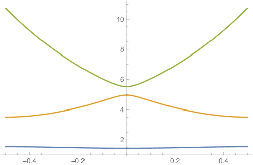
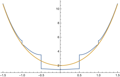
Figure 1: The first three energy bands of the quantum Mathieu equation for $R=1$, $\hbar=\pi/2$, represented in the first Brillouin zone (left) and in the extended zone (right), where we also plot the dispersion relation $2\cosh(\hbar k)$ for the free theory.

The central equation can be also used to solve for the band spectrum analytically, in terms of a power series. In the case of the Mathieu equation, this is nicely explained in section 2 of slater . This analysis can be easily extended to the quantum Mathieu operator. There are two different cases, depending on whether the quasi-momentum is in the interior or at the edges of the bands. If $k$ is an interior value, we can write the following ansatz for the band energy,

$$\epsilon(k,\hbar,R)=2\cosh(k\hbar)+\sum_{\ell\geq 1}\epsilon_{\ell}(k,\hbar)R^{2\ell},$$ (4.70)

where the first term is the dispersion relation for the free theory. We will now assume the normalization condition that $c_{k}=1$ for a fixed $k$, and that

$$c_{k\pm n}=R^{n}\sum_{\ell\geq 0}c^{(\ell)}_{\pm n}(k)R^{2\ell}.$$ (4.71)

The central equation for $k\pm 1$ and at leading order in $R$ gives

$$\left(2\cosh(k\pm 1)\hbar-2\cosh(k\hbar)\right)Rc^{(0)}_{\pm 1}(k)+R+{\cal O}(R^{2})=1,$$ (4.72)

so we find

$$c^{(0)}_{\pm 1}(k)=-{1\over 2\cosh(k\pm 1)\hbar-2\cosh(k\hbar)}.$$ (4.73)

In addition, by using the central equation for $k$, we find at leading order

$$\epsilon_{1}(k,\hbar)=c^{(0)}_{1}(k)+c^{(0)}_{-1}(k)={(Q_{2}^{1/2}+Q_{2}^{-1/2})Q_{1}{R^{-2}}\over\left(q^{1/2}Q_{2}-q^{-1/2}\right)\left(q^{-1/2}Q_{2}-q^{1/2}\right)},$$ (4.74)

with

$$Q_{1}=R^{2}{\rm e}^{2k\hbar},\quad Q_{2}={\rm e}^{2k\hbar},\quad q={\rm e}^{-\hbar}.$$ (4.75)

In particular, (4.74) reproduces precisely the first term in the expansion of $W(Q_{1},Q_{2},q)$ as computed by instanton calculus in section 3. It can be easily checked that this is also the case for the next few higher order terms.

order	$\epsilon_{0}(0,2\pi,1)$
1	1.996251125995166296078333
3	1.996251152313733927269664
5	1.996251152313733933761514
Num	1.996251152313733933761514

Table 4: The energy $\epsilon(0,2\pi,1)$ for the quantum Mathieu equation at the center of the band, as computed from (4.76). The order denotes the number of terms retained in the expansion of $W(Q_{1},Q_{2},q)$ in powers of $Q_{1}$.

We conjecture that this is true to all orders in the series expansion (4.70), so that

$$\epsilon(k,\hbar,R)=W\left(R^{2}{\rm e}^{2k\hbar},{\rm e}^{2k\hbar},{\rm e}^{-\hbar}\right).$$ (4.76)

We can then use the quantum mirror map to compute the band energies. An example of such a calculation is shown in table 4. We also observe that the solution (4.76) gives the correct band energies for complex values of $\hbar$ as far as ${\rm Re}(\hbar)\neq 0$ .

The equation (4.76) gives an analytic expression for the band energies, in terms of a series expansion for $W(Q_{1},Q_{2},q)$ to obtain concrete results. This series is convergent, so we do not expect to have non-perturbative corrections to (4.76). It has however a finite radius of convergence. Let us consider for example the center of the first band $k=0$, where we expect the maximal difference w.r.t. the free theory. We have the following structure,

$$\epsilon_{\ell}(0,\hbar)={f_{\ell}(q)\over(q-1)^{4\ell-2}},$$ (4.77)

where $f_{\ell}(q)$ is regular at $q=1$. In addition, numerical experiments indicate that,

$$f_{\ell}(q)\sim(-1)^{\ell}(f(q))^{\ell},\qquad\ell\gg 1,$$ (4.78)

where $f(q)>0$ whenever $q\in(0,1]$. This means that the coefficients $\epsilon_{\ell}(0,\hbar)$ grow, for $\ell$ large, as

$$\epsilon_{\ell}(0,\hbar)\sim\left[-{f(q)\over(q-1)^{4}}\right]^{\ell},$$ (4.79)

so the radius of convergence of this series is approximately given by

$$R^{2}\sim{(q-1)^{4}\over f(q)}.$$ (4.80)

This goes to zero as $\hbar\to 0$, so we don’t expect convergence for small values of $\hbar$, as we indeed observe numerically by computing the coefficients of (4.70) to high order. Nevertheless, since the series is alternating, it is expected that it can be resummed to a convergent function on the positive real axis of $R$. In particular, the convergence of (4.70) as $\hbar\to 0$ can be remarkably improved by using standard algorithms such as Padé approximants or Shanks transformations (see for example bender-book ). Let us illustrate this in one example, namely $k=0$ and $\hbar=\pi/3$. It is useful to define the truncated series

$$\epsilon^{(N)}[R]=\sum_{n\geq 0}^{N}\epsilon_{n}(0,{\pi/3})R^{2n}$$ (4.81)

and its Shanks transformation as

$$S(N,R)={\epsilon^{(N+1)}[R]\epsilon^{(N-1)}[R]-(\epsilon^{(N)}[R])^{2}\over\epsilon^{(N+1)}[R]-2\epsilon^{(N)}[R]+\epsilon^{(N-1)}[R]}.$$ (4.82)

Likewise we denote by

$$S_{n}(N,R),\quad N>n$$ (4.83)

the quantity obtained after applying $n$ times the Shanks transformation. For instance

$$S_{2}(N,R)={S({N+1},R)S(N-1,R)-(S(N,R))^{2}\over S({N+1},R)-2S({N},R)+S({N-1},R)}.$$ (4.84)

For $R=1$ (4.81) diverges at large $N$ as expected from (4.80) and shown in the first column of Table 5. Nevertheless by applying Shanks transformation repeatedly we can improve the convergence remarkably as shown for instance in Table 5.

$N$	$\epsilon^{(N)}[1]$	$S_{3}(N+3,1)$	$S_{6}(N+6,1)$	$S_{9}(N+9,1)$
1	0.334	1.0228922	1.0201454	1.02014601733678
2	2.423	1.0187015	1.0201458	1.02014600931881
3	-3.038	1.0212857	1.0201461	1.02014600851393
4	14.864	1.0188895	1.0201458	1.02014600944477
5	-50.900	1.0219159	1.0201462	1.02014600942947
Num				1.02014600942838

Table 5: The truncated (divergent) series (4.81) for $k=0$, $\hbar=\pi/3$, $R=1$ together with its $3^{\rm rd}$, $6^{\rm th}$ and $9^{\rm th}$ Shanks transform. In the last line the numerical value obtained by truncating the matrix equation is given.

The above solution for the energies (4.76) is valid in the interior of the band. As in the standard Mathieu equation, there are poles at the edges of the bands, i.e. when $k=\pm n/2$, $n\in{\mathbb{Z}}_{>0}$ (the poles at $k=\pm 1/2$ are manifest in (4.74)). This case has then to be treated separately, and we can follow again the methods of slater . To solve the central equation at the edges we have to change the ansatz (4.71), (4.70). We fix $k={1/2}$ at the edge of the Brillouin zone and we consider the following ansatz

$$\epsilon(\alpha,{1/2},\hbar,R)=2\cosh(\hbar/2)+\sum_{\ell\geq 1}\epsilon_{\ell}(\alpha,{1/2},\hbar)R^{\ell},$$ (4.85)

with

$$c_{1/2}=c^{(1/2)}_{0}=1,\quad c^{(1/2)}_{-1}=\alpha,\quad\alpha^{2}=1$$ (4.86)

$$c^{(1/2)}_{n}=R^{n}\sum_{\ell\geq 0}d^{\ell}_{n}R^{\ell},\quad n>0.$$ (4.87)

By solving (4.68) with this ansatz we find

$$\epsilon\left(\alpha,1/2,\hbar,R\right)=2\cosh\left(\frac{\hbar}{2}\right)+\alpha R+\frac{R^{2}}{2\cosh\left(\frac{\hbar}{2}\right)-2\cosh\left(\frac{3\hbar}{2}\right)}-\frac{\alpha R^{3}}{4\left(\cosh\left(\frac{\hbar}{2}\right)-\cosh\left(\frac{3\hbar}{2}\right)\right)^{2}}$$ (4.88)

$$-\frac{R^{4}\text{csch}^{3}\left(\frac{\hbar}{2}\right)\text{csch}^{3}(\hbar)}{128\cosh(\hbar)+64}+\frac{\alpha R^{5}(4\cosh(\hbar)+4\cosh(2\hbar)+3)\coth^{2}\left(\frac{\hbar}{2}\right)\text{csch}^{6}(\hbar)}{64(2\cosh(\hbar)+1)^{2}}+\mathcal{O}(R^{6}).$$

By setting $\alpha=-1$ we obtain the energy at the edge of the first band, while $\alpha=1$ gives the energy at the edge of the second band. Some results are shown in Table 6 and Table 7 and are in perfect agreement with the numerical computations.

order	$\epsilon\left(-1,{1\over 2},2\pi,1\right)$
1	22.1839065510430412555035041051
3	22.1838257067966848185142066748
5	22.1838257067966837480949560885
7	22.1838257067966837481053206977
Num	22.1838257067966837481053206975

Table 6: The energy $\epsilon\left(-1,{1\over 2},2\pi,1\right)$ for the quantum Mathieu equation at the edge of the first band, as computed from (4.88). The order denotes the number of terms retained in the expansion of $\epsilon\left(-1,{1\over 2},2\pi,R\right)$ in powers of $R$.

order	$\epsilon\left(1,{1\over 2},2\pi,1\right)$
1	24.18390655104304125550350410512
3	24.18382569372298652860218359466
5	24.18382569372298562878563284976
7	24.18382569372298562879599690871
Num	24.18382569372298562879599690846

Table 7: The energy $\epsilon\left(1,{1\over 2},2\pi,1\right)$ for the quantum Mathieu equation at the edge of the second band, as computed from (4.88). The order denotes the number of terms retained in the expansion of $\epsilon\left(1,{1\over 2},2\pi,R\right)$ in powers of $R$.

Notice that for $k=-{1\over 2}<0$ one has to replace the ansatz (4.87) by

$$c_{1/2}=c^{(1/2)}_{0}=1,\quad c^{(1/2)}_{1}=\alpha$$ (4.89)

$$c^{(1/2)}_{-n}=R^{n}\sum_{\ell\geq 0}d^{\ell}_{n}R^{\ell},\quad n>0.$$ (4.90)

However, at the end the result is the same, namely $\epsilon\left(\alpha,{1\over 2},\hbar,R\right)=\epsilon\left(\alpha,-{1\over 2},\hbar,R\right)$, as expected. We note that the solution (4.88) also holds for complex values of $\hbar$ as far as $\rm{Re}(\hbar)\neq 0$. Other values of $k$, corresponding to other edges of the bands, can be worked out similarly.

The series (4.85) is convergent with a finite radius of convergence, so we do not expect to have non-perturbative corrections. Numerically we observe a behaviour similar to (4.79), with a zero radius of convergence as $\hbar\rightarrow 0$. As before, we can improve the convergence by using standard algorithmss. For the series (4.85), the Padé approximant turns out to be well suited. An example is shown on Table 8. We use the same convention as in gmz for the Padé approximant.

$n$	$P_{n}^{\epsilon}(1)$
10	0.5156117750532916
20	0.5205803657529506
30	0.5205897527191174
40	0.5205897346606964
50	0.5205897353650857
55	0.5205897353651356
Num	0.5205897353651301

Table 8: The Padé approximant of order $n$ of for the series (4.85) with $k=1/2$ , $\hbar={\pi/6}$, $R=1$. We computed the coefficients in the series expansion (4.85) up to $R^{56}$.

Finally, we note that the even powers of $R$ in (4.85) can be obtained from the Wilson loop as

$$\sum_{n\geq 0}\epsilon_{2n}(\alpha,1/2,\hbar)R^{2n}={\rm{Res}}_{k=1/2}\left[W({\rm e}^{2k\hbar}R^{2},{\rm e}^{2k\hbar},{\rm e}^{-\hbar})(k-1/2)^{-1}\right].$$ (4.91)

It would be interesting to see whether there is a similar interpretation for the odd powers of $R$ in (4.85).

4.2 Four dimensional limit

In order to recover the Mathieu equation (4.62) from the quantum Mathieu equation (4.60) one has to implement the standard four dimensional limit, i.e. we replace

$$\hbar\to{\beta\hbar},\quad R\to\beta^{2}R,$$ (4.92)

and we take the limit $\beta\rightarrow 0$. Then, away from the edges of the bands, we obtain the well-known result expressing the band energies for the Mathieu equation in terms of the NS free energy of the $SU(2)$, ${\cal N}=2$ theory, namely (see for example he-miao ; kpt ; basar-dunne ; du-mathieu )

$$u(k,R,\hbar) =k^{2}\hbar^{2}-\Lambda\partial_{\Lambda}F^{\rm NS}(\Lambda,k\hbar,{\rm i}\hbar)$$ (4.93)

where we set $\Lambda=R^{2}$, and

$$F^{\rm NS}(\Lambda,a,\hbar)=-\frac{2\Lambda}{4a^{2}+\hbar^{2}}+\frac{\Lambda^{2}\left(7\hbar^{2}-20a^{2}\right)}{4\left(a^{2}+\hbar^{2}\right)\left(4a^{2}+\hbar^{2}\right)^{3}}+\mathcal{O}(\Lambda^{4}).$$ (4.94)

These results can be easily obtained by solving the central equation for (4.62) instead of taking the four dimensional limit (4.92). More precisely, the central equation for (4.62) reads

$$\hbar^{2}\left(k+{2\pi\over a}\ell\right)^{2}c_{\ell}^{(k)}+R\left(c^{(k)}_{\ell-1}+c^{(k)}_{\ell+1}\right)=u(k,R,\hbar)c_{\ell}^{(k)}.$$ (4.95)

By solving (4.95) at the edge of the first zone, i.e. for $k=1/2$, one finds slater ; mattab

$$u(1/2,R,\hbar)=u_{o}(\alpha,1/2,R,\hbar)+u_{e}(1/2,R,\hbar),$$ (4.96)

where $u_{e,o}$ are the even and odd powers of $R$, respectively. They have the explicit expression,

$$u_{o}(\alpha,1/2,R,\hbar) =R\alpha-\alpha\frac{R^{3}}{4\hbar^{4}}+\alpha\frac{11R^{5}}{144\hbar^{8}}+\alpha\frac{55R^{7}}{2304\hbar^{12}}+\cdots$$ (4.97)

$$u_{e}(1/2,R,\hbar) ={1\over 4}\hbar^{2}-\frac{R^{2}}{2\hbar^{2}}-\frac{R^{4}}{24\hbar^{6}}+\frac{49R^{6}}{576\hbar^{10}}+\cdots$$

By choosing $\alpha=-1$ one obtains the energy at the edge of the first band, while $\alpha=1$ gives the energy at the edge of the second band. As in the quantum Mathieu case, the even powers are still determined by the NS free energy. Indeed, one has

$$u_{e}(1/2,R,\hbar)={\rm Res}_{k=1/2}\left({u(k,R,\hbar)\over k-1/2}\right)={\rm Res}_{k=1/2}\left({k^{2}\hbar^{2}-\Lambda\partial_{\Lambda}F^{\rm NS}(\Lambda,k\hbar,{\rm i}\hbar)\over k-1/2}\right)\biggl{|}_{\Lambda=R^{2}}.$$ (4.98)

Again, it would be interesting to find an expression for the odd powers $u_{o}(\alpha,1/2,R,\hbar)$ in terms of gauge theory.

As a final observation, we note that, as in the case of quantum Mathieu equation, the series (4.96), (4.93) have a finite radius of convergence which goes to zero at $\hbar=0$. Nevertheless, one can also use Padé approximants to calculate the band energies.

5 Conclusions

In this paper we have taken the first steps to extend the TS/ST correspondence, as formulated in ghm ; cgm , to complex values of the Planck constant. We have noted that, at least when the toric CY engineers a 5d gauge theory, one can resum the series appearing in the exact quantization condition, in the form given in wzh . The results obtained in this way are in agreement with numerical calculations of the spectrum. One interesting outcome of our computations is that the non-perturbative effects detected in ghm ; cgm are crucial to obtain the correct results, even in situations where the all-orders WKB quantization condition of ns makes sense.

Clearly, there are many problems that one should address in order to have a full understanding of the complex side of the TS/ST correspondence. First of all, our results cover a small subset of all toric geometries, namely those directly related to gauge theories. For other geometries, like local ${\mathbb{P}}^{2}$, it is not clear how to resum the (refined) topological free energies, the grand potential and the quantum mirror map, in order to obtain convergent expansions. We should also note that, when $\hbar$ is real, the correspondence allows one to calculate the spectral traces and the spectral determinant of the operators. It would be interesting to see how this can be achieved in the complex case, even in examples related to gauge theories.

In this paper we have also considered other slices in the quantization of the mirror cuve, focusing for simplicity in the quantum Mathieu operator associated to local ${\mathbb{F}}_{0}$. The solution for the resulting band structure only involves the quantum mirror map and is much simpler than the solution of the trace class operators considered in ghm . The underlying reason, as pointed out in basar-dunne , is that we can regard the full periodic potential as a perturbation of a free particle on a circle. This leads to the convergent expansion (4.70), which is nothing but the quantum mirror map. Non-perturbative effects are not required to compute the energies of the bands, in contrast to what happens in the quantization scheme of ghm , where these effects are crucial. Since the expansions break down at the edges, one can however consider the energy splitting of the bands as some sort of non-perturbative effect, as advocated in avron-simon ; basar-dunne ; du-mathieu for the standard Mathieu equation. It would be interesting to study the splitting for the quantum Mathieu equation from that point of view.

The analysis of the operators along “imaginary” slices should be extended to more general geometries. One could also study operators obtained by going to the imaginary slices for both ${\mathsf{x}}$ and $\mathsf{p}$. In the case of local ${\mathbb{F}}_{0}$, this gives the “fully periodic” operator

$${\mathsf{O}}=2\cos(\mathsf{p})+2R\cos({\mathsf{x}}).$$ (5.99)

It is easy to see that this is equivalent to the Harper operator, leading to the famous Hofstadter butterfly. It has been observed that the quantum geometry of local ${\mathbb{F}}_{0}$ is closely related to some aspects of this problem butterfly . It would be interesting to see whether topological string theory sheds further light on the subtle spectral properties of the Harper operator.

Appendix A The grand potential

In this section we review the definition of the topological string grand potential. For this we first need to introduce various quantities appearing in topological string theory and in quantum geometry. We follow cgm ; mmrev , where more details and references can be found.

Let $X$ be a toric CY geometry as in section 2. It is convenient to write the “true” complex moduli (2.1) of $X$ as

$$\kappa_{i}={\rm e}^{\mu_{i}},$$ (A.100)

and to introduce the Batyrev coordinates $z_{i}$ such that

$$-\log\,z_{i}=\sum_{j=1}^{g_{\Sigma}}C_{ij}\mu_{j}+\sum_{k=1}^{r_{\Sigma}}\alpha_{ik}\log{\xi_{k}},\qquad i=1,\cdots,n_{\Sigma},$$ (A.101)

where $C_{ij}$ is a $n_{\Sigma}\times g_{\Sigma}$ matrix which is determined by the toric data of $X$ as explained in kpsw . The Kahler moduli $t_{i}$ and the Batyrev coordinates are related by the mirror map

$$-t_{i}=\log z_{i}+\Pi_{i}(\bf z),$$ (A.102)

where $\Pi_{i}$ is a power series in $z_{j}$. We also denote $Q_{i}={\rm e}^{-t_{i}}.$ As explained in acdkv , we can promote (A.102) to a quantum mirror map

$$-t_{i}(\hbar)=\log z_{i}+\Pi_{i}(\bf z,\hbar).$$ (A.103)

We introduce the topological string free energy

$$F^{\rm top}\left({\bf t},g_{s}\right)={1\over 6g_{s}^{2}}a_{ijk}t_{i}t_{j}t_{k}+b_{i}t_{i}+F^{\rm GV}\left({\bf t},g_{s}\right)$$ (A.104)

where

$$F^{\rm GV}\left({\bf t},g_{s}\right)=\sum_{g\geq 0}\sum_{\bf d}\sum_{w=1}^{\infty}{1\over w}n_{g}^{{\bf d}}\left(2\sin{wg_{s}\over 2}\right)^{2g-2}{\rm e}^{-w{\bf d}\cdot{\bf t}}$$ (A.105)

is written in terms of the Gopakumar–Vafa (GV) invariants $n_{g}^{{\bf d}}$ of the underlying geometry $X$. Similarly, the Nekrasov–Shatahsvili (NS) free energy of $X$ is defined as

$$F^{\rm NS}({\bf t},\hbar)={1\over 6\hbar}a_{ijk}t_{i}t_{j}t_{k}+b^{\rm NS}_{i}t_{i}\hbar+\sum_{j_{L},j_{R}}\sum_{w,{\bf d}}N^{{\bf d}}_{j_{L},j_{R}}\frac{\sin\frac{\hbar w}{2}(2j_{L}+1)\sin\frac{\hbar w}{2}(2j_{R}+1)}{2w^{2}\sin^{3}\frac{\hbar w}{2}}{\rm e}^{-w{\bf d}\cdot{\bf t}},$$ (A.106)

where $N^{{\bf d}}_{j_{L},j_{R}}$ are refined BPS invariants. We also need a B-field satisfying

$$(-1)^{2j_{L}+2j_{R}+1}=(-1)^{{\bf B}\cdot{\bf d}},$$ (A.107)

for the indices labelling non-vanishing invariants $N^{{\bf d}}_{j_{L},j_{R}}$.

The topological string grand potential is defined as

$$\mathsf{J}_{X}(\boldsymbol{\mu},\boldsymbol{\xi},\hbar)=\mathsf{J}^{\rm WKB}_{X}(\boldsymbol{\mu},\boldsymbol{\xi},\hbar)+\mathsf{J}^{\rm WS}_{X}(\boldsymbol{\mu},\boldsymbol{\xi},\hbar),$$ (A.108)

where

$$\mathsf{J}^{\rm WS}_{X}(\boldsymbol{\mu},\boldsymbol{\xi},\hbar)=F^{\rm GV}\left({2\pi\over\hbar}{\bf t}(\hbar)+\pi{\rm i}{\bf B},{4\pi^{2}\over\hbar}\right),$$ (A.109)

and

$$\mathsf{J}^{\rm WKB}_{X}(\boldsymbol{\mu},\boldsymbol{\xi},\hbar)={t_{i}(\hbar)\over 2\pi}{\partial F^{\rm NS}({\bf t}(\hbar),\hbar)\over\partial t_{i}}+{\hbar^{2}\over 2\pi}{\partial\over\partial\hbar}\left({F^{\rm NS}({\bf t}(\hbar),\hbar)\over\hbar}\right)+{2\pi\over\hbar}b_{i}t_{i}(\hbar)+A({\boldsymbol{\xi}},\hbar).$$ (A.110)

Here, $A({\boldsymbol{\xi}},\hbar)$ is a moduli-independent contribution which can be related to the contribution of constant maps in topological string theory.

We will also use the following notation

$$F^{\rm NS,inst}({\bf t},\hbar)=\sum_{j_{L},j_{R}}\sum_{w,{\bf d}}N^{{\bf d}}_{j_{L},j_{R}}\frac{\sin\frac{\hbar w}{2}(2j_{L}+1)\sin\frac{\hbar w}{2}(2j_{R}+1)}{2w^{2}\sin^{3}\frac{\hbar w}{2}}{\rm e}^{-w{\bf d}\cdot{\bf t}},$$ (A.111)

as well as the twisted free energy

$${\widehat{F}}^{\rm NS,inst}({\bf t},\hbar)=\sum_{j_{L},j_{R}}\sum_{w,{\bf d}}N^{{\bf d}}_{j_{L},j_{R}}\frac{\sin\frac{\hbar w}{2}(2j_{L}+1)\sin\frac{\hbar w}{2}(2j_{R}+1)}{2w^{2}\sin^{3}\frac{\hbar w}{2}}{\rm e}^{-w{\bf d}\cdot\left({\bf t+{\rm i}\pi{\bf B}}\right)},$$ (A.112)

$${\widehat{F}}^{\rm NS}({\bf t},\hbar)={1\over 6\hbar}a_{ijk}t_{i}t_{j}t_{k}+b^{\rm NS}_{i}t_{i}\hbar+{\widehat{F}}^{\rm NS,inst}({\bf t},\hbar),$$ (A.113)

and the twisted quantum mirror map

$$-{\widehat{t}}_{i}(\hbar)=\log z_{i}+\Pi_{i}(\bf z_{B},\hbar),$$ (A.114)

where ${\bf z_{B}}=(z_{1}(-1)^{B_{1}},\cdots,z_{g_{\Sigma}+r_{\Sigma}}(-1)^{B_{g_{\Sigma}+r_{\Sigma}}})$.

References

- (1) M. Aganagic, R. Dijkgraaf, A. Klemm, M. Mariño and C. Vafa, Topological strings and integrable hierarchies, Commun.Math.Phys. 261 (2006) 451–516, [hep-th/0312085].
- (2) N. A. Nekrasov and S. L. Shatashvili, Quantization of Integrable Systems and Four Dimensional Gauge Theories, 0908.4052.
- (3) A. Mironov and A. Morozov, Nekrasov Functions and Exact Bohr-Sommerfeld Integrals, JHEP 1004 (2010) 040, [0910.5670].
- (4) M. Aganagic, M. C. Cheng, R. Dijkgraaf, D. Krefl and C. Vafa, Quantum Geometry of Refined Topological Strings, JHEP 1211 (2012) 019, [1105.0630].
- (5) M. Mariño and P. Putrov, ABJM theory as a Fermi gas, J.Stat.Mech. 1203 (2012) P03001, [1110.4066].
- (6) Y. Hatsuda, S. Moriyama and K. Okuyama, Exact Results on the ABJM Fermi Gas, JHEP 1210 (2012) 020, [1207.4283].
- (7) Y. Hatsuda, S. Moriyama and K. Okuyama, Instanton Effects in ABJM Theory from Fermi Gas Approach, JHEP 1301 (2013) 158, [1211.1251].
- (8) F. Calvo and M. Mariño, Membrane instantons from a semiclassical TBA, JHEP 1305 (2013) 006, [1212.5118].
- (9) Y. Hatsuda, S. Moriyama and K. Okuyama, Instanton Bound States in ABJM Theory, JHEP 1305 (2013) 054, [1301.5184].
- (10) Y. Hatsuda, M. Mariño, S. Moriyama and K. Okuyama, Non-perturbative effects and the refined topological string, JHEP 1409 (2014) 168, [1306.1734].
- (11) J. Kallen and M. Mariño, Instanton effects and quantum spectral curves, Annales Henri Poincare 17 (2016) 1037–1074, [1308.6485].
- (12) M.-x. Huang and X.-f. Wang, Topological Strings and Quantum Spectral Problems, JHEP 1409 (2014) 150, [1406.6178].
- (13) S. Codesido, A. Grassi and M. Mariño, Exact results in N=8 Chern-Simons-matter theories and quantum geometry, JHEP 1507 (2015) 011, [1409.1799].
- (14) A. Grassi, Y. Hatsuda and M. Mariño, Topological Strings from Quantum Mechanics, Ann. Henri Poincaré (2016) , [1410.3382].
- (15) S. Codesido, A. Grassi and M. Mariño, Spectral Theory and Mirror Curves of Higher Genus, Annales Henri Poincare 18 (2017) 559–622, [1507.02096].
- (16) M. Mariño, Spectral Theory and Mirror Symmetry, 1506.07757.
- (17) R. Kashaev and M. Mariño, Operators from mirror curves and the quantum dilogarithm, Commun. Math. Phys. 346 (2016) 967, [1501.01014].
- (18) M. Mariño and S. Zakany, Matrix models from operators and topological strings, Annales Henri Poincare 17 (2016) 1075–1108, [1502.02958].
- (19) Y. Hatsuda, Spectral zeta function and non-perturbative effects in ABJM Fermi-gas, JHEP 11 (2015) 086, [1503.07883].
- (20) R. Kashaev, M. Mariño and S. Zakany, Matrix models from operators and topological strings, 2, Annales Henri Poincare 17 (2016) 2741–2781, [1505.02243].
- (21) X. Wang, G. Zhang and M.-x. Huang, New Exact Quantization Condition for Toric Calabi-Yau Geometries, Phys. Rev. Lett. 115 (2015) 121601, [1505.05360].
- (22) J. Gu, A. Klemm, M. Mariño and J. Reuter, Exact solutions to quantum spectral curves by topological string theory, JHEP 10 (2015) 025, [1506.09176].
- (23) Y. Hatsuda, Comments on Exact Quantization Conditions and Non-Perturbative Topological Strings, 1507.04799.
- (24) A. Laptev, L. Schimmer and L. A. Takhtajan, Weyl type asymptotics and bounds for the eigenvalues of functional-difference operators for mirror curves, Geom. Funct. Anal. 26 (2016) 288–305, [1510.00045].
- (25) Y. Hatsuda and M. Mariño, Exact quantization conditions for the relativistic Toda lattice, JHEP 05 (2016) 133, [1511.02860].
- (26) S. Franco, Y. Hatsuda and M. Mariño, Exact quantization conditions for cluster integrable systems, J. Stat. Mech. 1606 (2016) 063107, [1512.03061].
- (27) K. Okuyama and S. Zakany, TBA-like integral equations from quantized mirror curves, JHEP 03 (2016) 101, [1512.06904].
- (28) G. Bonelli, A. Grassi and A. Tanzini, Seiberg–Witten theory as a Fermi gas, Lett. Math. Phys. 107 (2017) 1–30, [1603.01174].
- (29) A. Grassi, Spectral determinants and quantum theta functions, J. Phys. A49 (2016) 505401, [1604.06786].
- (30) A.-K. Kashani-Poor, Quantization condition from exact WKB for difference equations, JHEP 06 (2016) 180, [1604.01690].
- (31) A. Sciarappa, Bethe/Gauge correspondence in odd dimension: modular double, non-perturbative corrections and open topological strings, JHEP 10 (2016) 014, [1606.01000].
- (32) Y. Sugimoto, Geometric transition in the nonperturbative topological string, Phys. Rev. D94 (2016) 055010, [1607.01534].
- (33) Y. Hatsuda, H. Katsura and Y. Tachikawa, Hofstadter’s butterfly in quantum geometry, New J. Phys. 18 (2016) 103023, [1606.01894].
- (34) M. Mariño and S. Zakany, Exact eigenfunctions and the open topological string, J. Phys. A50 (2017) 325401, [1606.05297].
- (35) K. Sun, X. Wang and M.-x. Huang, Exact Quantization Conditions, Toric Calabi-Yau and Nonperturbative Topological String, JHEP 01 (2017) 061, [1606.07330].
- (36) S. Codesido, J. Gu and M. Mariño, Operators and higher genus mirror curves, JHEP 02 (2017) 092, [1609.00708].
- (37) A. Grassi and J. Gu, BPS relations from spectral problems and blowup equations, 1609.05914.
- (38) R. Couso-Santamaría, M. Mariño and R. Schiappa, Resurgence Matches Quantization, J. Phys. A50 (2017) 145402, [1610.06782].
- (39) J. Gu, M.-x. Huang, A.-K. Kashani-Poor and A. Klemm, Refined BPS invariants of 6d SCFTs from anomalies and modularity, 1701.00764.
- (40) Y. Hatsuda, Y. Sugimoto and Z. Xu, Calabi-Yau geometry and electrons on 2d lattices, Phys. Rev. D95 (2017) 086004, [1701.01561].
- (41) G. Bonelli, A. Grassi and A. Tanzini, New results in theories from non-perturbative string, 1704.01517.
- (42) A. Sciarappa, Exact relativistic Toda chain eigenfunctions from Separation of Variables and gauge theory, 1706.05142.
- (43) M. Mariño and S. Zakany, Wavefunctions, integrability, and open strings, 1706.07402.
- (44) A. Iqbal and A.-K. Kashani-Poor, Instanton counting and Chern-Simons theory, Adv. Theor. Math. Phys. 7 (2003) 457–497, [hep-th/0212279].
- (45) A. Iqbal and A.-K. Kashani-Poor, SU(N) geometries and topological string amplitudes, Adv. Theor. Math. Phys. 10 (2006) 1–32, [hep-th/0306032].
- (46) N. A. Nekrasov, Seiberg-Witten prepotential from instanton counting, Adv.Theor.Math.Phys. 7 (2004) 831–864, [hep-th/0206161].
- (47) M. Aganagic, A. Klemm, M. Mariño and C. Vafa, The Topological vertex, Commun.Math.Phys. 254 (2005) 425–478, [hep-th/0305132].
- (48) W. He and Y.-G. Miao, Mathieu equation and Elliptic curve, Commun. Theor. Phys. 58 (2012) 827–834, [1006.5185].
- (49) G. Başar and G. V. Dunne, Resurgence and the Nekrasov-Shatashvili limit: connecting weak and strong coupling in the Mathieu and Lamé systems, JHEP 02 (2015) 160, [1501.05671].
- (50) G. V. Dunne and M. Unsal, WKB and Resurgence in the Mathieu Equation, 1603.04924.
- (51) M.-X. Huang, A. Klemm and M. Poretschkin, Refined stable pair invariants for E-, M- and -strings, JHEP 1311 (2013) 112, [1308.0619].
- (52) M.-x. Huang, A. Klemm, J. Reuter and M. Schiereck, Quantum geometry of del Pezzo surfaces in the Nekrasov-Shatashvili limit, JHEP 1502 (2015) 031, [1401.4723].
- (53) G. Bonelli, K. Maruyoshi and A. Tanzini, Quantum Hitchin Systems via beta-deformed Matrix Models, 1104.4016.
- (54) H. Nakajima and K. Yoshioka, Instanton counting on blowup. II. K-theoretic partition function, math/0505553.
- (55) A. B. Goncharov and R. Kenyon, Dimers and cluster integrable systems, 1107.5588.
- (56) S. H. Katz, A. Klemm and C. Vafa, Geometric engineering of quantum field theories, Nucl.Phys. B497 (1997) 173–195, [hep-th/9609239].
- (57) M. Taki, Refined Topological Vertex and Instanton Counting, JHEP 03 (2008) 048, [0710.1776].
- (58) A. Iqbal, C. Kozcaz and C. Vafa, The Refined topological vertex, JHEP 0910 (2009) 069, [hep-th/0701156].
- (59) M. A. Bershtein and A. I. Shchechkin, q-deformed Painlevé function and q-deformed conformal blocks, J. Phys. A50 (2017) 085202, [1608.02566].
- (60) M. Bullimore and H.-C. Kim, The Superconformal Index of the (2,0) Theory with Defects, JHEP 05 (2015) 048, [1412.3872].
- (61) M. Bullimore, H.-C. Kim and P. Koroteev, Defects and Quantum Seiberg-Witten Geometry, JHEP 05 (2015) 095, [1412.6081].
- (62) R. M. Kashaev and S. M. Sergeev, Spectral equations for the modular oscillator, 1703.06016.
- (63) D. Krefl, Non-Perturbative Quantum Geometry III, JHEP 08 (2016) 020, [1605.00182].
- (64) N. W. Ashcroft and N. D. Mermin, Solid state physics. Harcourt College Publishers, 1976.
- (65) J. Slater, A soluble problem in energy bands, Phys. Rev. 87 (1952) 807.
- (66) C. M. Bender and S. A. Orszag, Advanced mathematical methods for scientists and engineers. Springer-Verlag, 1999.
- (67) A. Grassi, M. Mariño and S. Zakany, Resumming the string perturbation series, JHEP 1505 (2015) 038, [1405.4214].
- (68) A.-K. Kashani-Poor and J. Troost, Pure super Yang-Mills and exact WKB, JHEP 08 (2015) 160, [1504.08324].
- (69) Tables relating to Mathieu functions. Columbia University Press, New York, 1951.
- (70) J. Avron and B. Simon, The asymptotics of the gap in the mathieu equation, Annals of Physics 134 (1981) 76–84.
- (71) A. Klemm, M. Poretschkin, T. Schimannek and M. Westerholt-Raum, Direct Integration for Mirror Curves of Genus Two and an Almost Meromorphic Siegel Modular Form, 1502.00557.