Cosmological investigation of multi-frequency VLBI observations of ultra-compact structure in $z\sim 3$ radio quasars

Abstract

In this paper, we use multi-frequency angular size measurements of 58 intermediate-luminosity quasars reaching the redshifts $z\sim 3$ and demonstrate that they can be used as standard rulers for cosmological inference. Our results indicate that, for the majority of radio-sources in our sample their angular sizes are inversely proportional to the observing frequency. From the physical point of view it means that opacity of the jet is governed by pure synchrotron self-absorption, i.e. external absorption does not play any significant role in the observed angular sizes at least up to 43 GHz. Therefore, we use the value of the intrinsic metric size of compact milliarcsecond radio quasars derived in a cosmology independent manner from survey conducted at 2 GHz and rescale it properly according to predictions of the conical jet model. This approach turns out to work well and produce quite stringent constraints on the matter density parameter $\Omega_{m}$ in the flat $\Lambda$CDM model and Dvali-Gabadadze-Porrati braneworld model. The results presented in this paper pave the way for the follow up engaging multi-frequency VLBI observations of more compact radio quasars with higher sensitivity and angular resolution.

I Introduction

For some time, radio sources (extended FRIIb radio galaxies, radio loud quasars, etc.) have been proposed as standard rulers (Buchalter et al., 1998; Guerra & Daly, 1998; Guerra, Daly & Wan, 2000; Daly & Djorgovski, 2003) and hence as alternative cosmological probes complementary to standard candles (SN Ia) and anisotropies in the cosmic microwave background radiation (CMBR). One important class of such objects are ultra-compact radio-sources whose cores have angular sizes of order of milliarcseconds ($mas$) which could be measured by very-long-baseline interferometry (VLBI) (Kellermann, 1993; Gurvits, 1994). In the VLBI images, the core is usually identified with the most compact (often unresolved) feature with a substantial flux and flat spectrum across the radio band. More importantly, radio sources (especially quasars) can be observed up to very high redshifts, well beyond the observed redshift range of SNIa (Amanullah et al., 2010) limited to $z<2$. First attempts to constrain cosmological models using such kind of sources were due to Gurvits, Kellerman & Frey (1999), who compiled a data-set of 330 milliarcsecond radio sources containing various optical counterparts (radio galaxies, quasars, BL Lac etc.). A sub-sample containing 145 compact sources with little dependence of angular size on spectral index ($-0.38\leq\alpha\leq 0.18$) and luminosity $Lh^{2}\geq 10^{26}\;WHz^{-1}$ was also derived in their analysis, based on which all data points were distributed into twelve redshift bins and were extensively discussed in the literature (Vishwakarma, 2001; Zhu & Fujimoto, 2002; Chen & Ratra, 2003) as cosmological probes. However, the determination of the typical value of the linear size $l_{m}$ for this standard ruler (or even whether compact radio sources are indeed “true” standard rulers) was remaining an important problem to be solved (Vishwakarma, 2001; Cao et al., 2015). Based on the previous conclusion formulated in Cao et al. (2015), that mixed population of radio sources including different optical counterparts can not be treated as a “true” standard ruler, Cao et al. (2017a) demonstrated that only in the intermediate-luminosity radio quasars their compact structure displayed minimal dependence of the linear size on redshift and luminosity. Therefore they could serve as a cosmological standard ruler. Identifying 120 such intermediate-luminosity quasars allowed Cao et al. (2017b) to explore various cosmological models in the high redshift range ($z\sim 3.0$), a range which was difficult to access by other cosmological probes. Such quasar sample has also been extensively used to investigate other dynamical dark energy models (Li et al., 2017; Zheng et al., 2017) and modified gravity theories (Qi et al., 2017; Xu et al., 2017). This was done however, based on the results of a survey performed on a single frequency 2.29 GHz and a question might be raised whether this successful calibration of standard rulers is just by coincidence or has a broader scope of applications comprising VLBI surveys on other frequencies. The focus of this paper is to extend the previous analysis of Cao et al. (2017b) and investigate possible astrophysical applications of the multi-frequency angular-size measurements of 58 quasars covering redshifts $z=0.536-2.73$. More importantly, the angular size of ultra-compact structure depends on the observing frequency, due to synchrotron self-absorption of the radio core (absorption in the radio emitting plasma itself) and external absorption in the surrounding material (Blandford & Königl, 1979; Lobanov, 1998). Therefore, the measurements of the angular sizes at three or more frequencies can be used to study the physics of compact radio-emitting region.

Table 1: Compilation of intermediate-luminosity quasars from Pushkarev & Kovalev (2015). Quasars with flux density smaller than 1.0 Jy are written in bold. Column (1): source (name); Column (2): redshift; Column (3)-(8): angular size in milliarcseconds at 2, 5, 8, 15, 24, and 43 GHz, respectively.

Source	$z$	$\theta_{2}$	$\theta_{5}$	$\theta_{8}$	$\theta_{15}$	$\theta_{24}$	$\theta_{43}$	Source	$z$	$\theta_{2}$	$\theta_{5}$	$\theta_{8}$	$\theta_{15}$	$\theta_{24}$	$\theta_{43}$
J1256-0547	0.536	2.56	0.59	0.37	0.23	0.13	0.07	J1617+0246	1.339	1.91		0.33
J0407-1211	0.573	1.82		0.33				J0808+4052	1.42	0.83	0.43	0.15	0.06	0.12	0.07
J0922-3959	0.591	2		0.38				J1534+0131	1.435	1.24	0.86	0.43	0.18
J1642+3948	0.593	1.29	1.28	0.54	0.24	0.19		J1033-3601	1.455	1.08		0.48
J2332-4118	0.671	1.89		0.45				J2255+4202	1.476	0.99	0.52	0.39
J1800+7828	0.68	0.55	0.27	0.23	0.16	0.1	0.09	J2056-4714	1.489	2		0.59
J1357+1919	0.72	1.4	0.75	0.41	0.14	0.43		J0222-3441	1.49	0.98		0.45
J1637+4717	0.74	0.72		0.23	0.08			J1417+4607	1.554	1.7	1.63	0.74
J1239-1023	0.752	2.25	1.37	0.7				J2229-0832	1.56	0.82		0.18	0.11	0.07	0.04
J0728+6748	0.846	0.99		0.26				J0409-1238	1.563	0.81		0.22
J0917-2131	0.847	1.72		0.2				J0839+0319	1.57	1.7		0.49
J1215+3448	0.857	1.31	0.82	0.51				J1107-4449	1.598	2.84		0.9
J0538-4405	0.894	1.41		0.43				J1640+3946	1.66	0.64	0.28	0.27	0.12	0.08	0.05
J0539-1550	0.947	1.59		0.38				J0110-0741	1.776	1.85
J1937-3958	0.965	1.49		0.34				J1454-4012	1.81	2.17		0.46
J0239+0416	0.978	0.89		0.23	0.05			J1036-3744	1.821	1.37
J0132-1654	1.02	1.44	0.59	0.91	0.25			J0808-0751	1.837	1.18	1.23	0.29	0.1	0.07
J1516+1932	1.07	0.88		0.16	0.09	0.11		J0639+7324	1.85	1.44		0.26
J1337+5501	1.1	1.22	0.45	0.47				J1357-1527	1.89	0.96		0.23	0.14	0.12	0.07
J1213+1307	1.14	1.53						J0620-2515	1.9	0.84		1.09
J2331-1556	1.153	1.56	1.15	0.5	0.45			J1658+3443	1.937	1.82	0.47	0.57
J1441-3456	1.159	1.9						J1327+4326	2.08	0.94	0.41	0.57
J1955+5131	1.22	1.05	0.66	0.23	0.2			J2322+0812	2.09	2.06		1.14
J1153+8058	1.25	1.19		0.31	0.27	0.15		J1022+1853	2.136	1.94	2.39
J1023+3948	1.254	1.03	0.69	0.26	0.1			J0644-3459	2.165	3.28	0.57	0.91
J0516-1603	1.278	1.69		0.73				J1035-2011	2.198	1.81	0.89	0.5	0.41	0.21
J0406-3826	1.285	0.96		0.45				J2316-4041	2.448	1.19		0.21
J0710+4732	1.292	0.79	0.75	0.16	0.12	0.07		J0331-2524	2.685	1.77		0.2
J2314-3138	1.323	0.91		0.36				J0139+1753	2.73	1		0.72	0.23

II Methodology and observational Data

Standard ruler approach to measure cosmological distances (Sandage, 1988), is based on quite obvious geometric relation

$$\theta(z)=\frac{l_{m}}{D_{A}(z)}$$ (1)

between the intrinsic metric length $l_{m}$ of the standard ruler located at the redshift $z$, its observed angular size $\theta(z)$ and its angular diameter distance $D_{A}(z)$. The main problem here is to find a convincing population of standardizable rulers. In particular, metric sizes $l_{m}$ of compact radio sources may depend on their luminosity $L$ (i.e. on the central engine) and display evolutionary effects, i.e. may depend on $z$. As already mentioned, Cao et al. (2017a) using the parametrization $l_{m}=lL^{\beta}(1+z)^{n}$ capturing these effects, demonstrated that the linear size $l_{m}$ of compact structure in 120 intermediate-luminosity quasars observed at 2.29 GHz (later on we will denote this frequency as 2 GHz for short) displays negligible dependence both on redshift and luminosity ($|n|\simeq 10^{-3}$, $|\beta|\simeq 10^{-4}$).

In extragalactic jets, however, the apparent position of a bright narrow end depends on the observing frequency, owing to synchrotron self-absorption and external absorption. Considering that 10 pc is a typical radius at which AGN jets are apparently generated (Blandford & Rees, 1978), it is very important to investigate the relation between the observing frequency and the apparent linear size of compact structure. To be more specific, at any given frequency, the core is believed to be located in the region of the jet where the optical depth is $\tau=1$. In the conical jet model proposed by Blandford & Königl (1979), if we observe a given milliarcsecond source at different observing frequencies $\nu$, its observed size falls as the frequency increases (Marscher & Shaffer, 1980; O’Sullivan & Gabuzda, 2009), being proportional to $\nu^{-1}$. At this point, one should clarify the issue of reception frequency $\nu_{r}$ and the rest-frame frequency $\nu_{e}$. At first sight an expectation would be that angular sizes in corresponding angular-size vs. redshift diagrams should fall by an additional factor $(1+z)^{-1}$, because the rest-frame emitted frequency has to be greater than $\nu_{e}$ by a factor of $(1+z)$: $\nu_{e}=(1+z)\nu_{r}$, thus masking any cosmological effect. However, observations show behavior which is compatible with conventional cosmologies. The reason is almost certainly that there is a selection effect which is operating in our favor in this context. Namely, we are dealing with an ensemble of objects which may be intrinsically similar in their respective rest-frames, but appear to be very different in our frame. According to the unified model of active galactic nuclei and quasars (Antonucci, 1993, 2015), the underlying population consists of compact symmetric objects (Wilkinson et al., 1994), each comprising a central low-luminosity nucleus straddled by two oppositely-directed jets. Ultra-compact objects are identified as cases in which the jets are moving relativistically and are close to the line of sight, when Doppler boosting allows just that component which is moving towards the observer to be observed. Giving rise to the core-jet structure observed in typical VLBI images (Pushkarev & Kovalev, 2012), the core tends to act as the base of the jet instead of the nucleus (Blandford & Königl, 1979). Those jets which are closest to the line of sight appear to be the brightest. Following the analysis of Dabrowski et al. (1995), for a flux-limited radio sample, a larger Doppler boost factor D is required as $z$ increases, which will generate an approximately fixed ratio ${\cal D}/(1+z)$ and thus an approximately fixed rest-frame emitted frequency $(1+z)\nu_{r}/{\cal D}$. See Jackson (2004) for mathematical and astrophysical details.

Moreover, the dependence of the angular size ($\theta$) on spectral index ($\alpha$) which, if not considered, could also constitute a possible sources of systematics in the dispersion of the linear size ($l_{m}$). More specifically, following the simple consideration of self absorption arguments, radio sources with flat and inverted spectra tend to have smaller sizes and there is an obvious dependence of angular size on spectral index (see Fig. 7 of Gurvits, Kellerman & Frey (1999) for details). In view of this effect in the currently available sample, there have been arguments based on the restricted range of spectral indices (a flat segment of the $\theta-\alpha$ diagram $-0.38\leq\alpha\leq 0.18$) that elimination of the large compact steep spectrum sources and most compact inverted spectrum sources will better define compact sources as standard rulers (Gurvits, Kellerman & Frey, 1999). More importantly, as was noted in the same work, the remarkable feature of such selection criterion lies in the fact that lowest-redshift sources ($z<0.5$), which exhibit the highest deviation on the $\alpha-z$ diagram (Jackson, 2004), will be partially excluded from the final sample used for statistical analysis. Therefore, in this work we will adopt the same criterion of $\alpha$ and concentrate on compact radio quasars with flat spectral index.

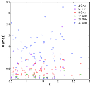
Figure 1: Angular size vs. redshift for the Pushkarev & Kovalev (2015) sample of 58 sources at six radio frequencies.

In our analysis, we turn to the more recent VLBI imaging observations based on better uv-coverage. Pushkarev & Kovalev (2015) presented the VLBI data of more than 3000 compact extragalactic radio sources observed at different frequencies, $\nu=2-43$ GHz. This sample, however, contains a wide class of extragalactic objects, belonging to different luminosity categories, including quasars, radio galaxies, and BL Lac objects. We identified 58 intermediate-luminosity quasars from the sub-sample constructed in Cao et al. (2017a), which have also been included in the Pushkarev & Kovalev (2015) sample. Fig. 1 displays the observed angular size against redshift in this sample. This way, we obtained a set of data – summarized in Table 1 – comprising angular sizes of flat spectrum cores in intermediate-luminosity radio quasars at six different radio frequencies: 2, 5, 8, 15, 24 and 43 GHz.

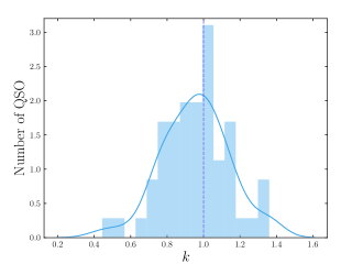
Figure 2: Distribution of $k$ parameter in our sample. Blue solid curve represents the best fitted continuous distribution function. Pure synchrotron self-absorption case ($k=1$) is denoted by the purple dashed line.

In order to use Eq.(1) for cosmological inference one needs to calibrate $l_{m}$. According to Blandford & Königl (1979) calibrated metric size of such standard ruler should depend on observing frequency in the same way as the observed angular size. Owing to synchrotron self-absorption of the radio core (absorption in the radio emitting plasma itself) and external absorption in the surrounding material, the angular size at any given observing frequency $\nu$ should scale as $\theta_{\nu}\propto\nu^{-k}$. The parameter $k$ representing the dependence of the angular size on frequency, is related to physics of the compact radio-emitting region: the shape of electron energy spectrum and the magnetic field and particle density distributions. Namely, (1) $k=1$ if the core is self-absorbed and in equipartition (Blandford & Königl, 1979); (2) $k>1$ if external absorption plays an important role (Lobanov, 1998). Therefore, the measurements of the angular sizes at three or more frequencies can be used for determining the value of $k$ and thus testing the Blandford & Königl (1979) jet model and its later modifications (Hutter & Mufson, 1986; Bloom & Marscher, 1996). Therefore, VLBI results obtained at other frequencies on the same sources as used in the current study should be used for verification of the results. We checked that frequency dependence of angular sizes in our sample is compatible with Blandford & Königl (1979) conical jet model. For each quasar, the best-fit $k$ parameter and its corresponding 1$\sigma$ uncertainty is determined through a $\chi^{2}$ minimization method. Following the previous analysis of a large sample of 140 mas compact radio sources (Cao et al., 2015), we have assumed a conservative 10% statistical uncertainty in the observed angular sizes. Fig. 2 displays the distribution of $k$ parameter in our sample of quasars. Best-fit probability distribution function (PDF) is represented by the blue solid curve.

One objection one might rise towards the proposed method is the rigid assumption of the Blandford & Königl (1979) conical jet model. Although there are some arguments supporting good consistency between the VLBI observations and the BK79 conical jet model in the earlier studies, which was done by using the recent multi-frequency core shift measurements of many compact radio sources (Lobanov, 1998; Kovalev et al., 2008, 2009; O’Sullivan & Gabuzda, 2009), one can expect the deviation from this standard jet model. Therefore, in the context of multi-frequency data, one can use the characteristic linear size at 2 GHz and scale it according to $l_{m}\propto\nu^{-k}$ to any other frequency. However, this model still requires that the quantity $k$ is constant, while as we see in Fig. 2 it has some distribution across the sample. Consequently in the following analysis we also performed fits assuming the linear relation: $k(z)=k_{0}+k_{1}z$ treating $k_{0}$ and $k_{1}$ as free parameters together with cosmological ones. We remark here that, considering the fact that the fixed ratio ${\cal D}/(1+z)$ is only expected to occur at the flux limit of the survey, it is mandatory to take this effect into consideration and verify its usability for cosmological test. Therefore, in the following analysis we will also use 30 quasars with flux density smaller than 1.0 Jy, a flux-density limit resulting in a sample observed with VLBI covering the full sky (Preston et al., 1985). This restricted sample is summarized in Table 1 where the names of quasars are given in bold.

Now a cosmological-model-independent method should be applied to derive the linear size of the compact structure in radio quasars at 2 GHz, by constructing angular diameter distances $D_{A}$ by means of GP-processed $H(z)$ measurements (Moresco et al., 2012; Zheng et al., 2016) from cosmic chronometers (Jimenez & Loeb, 2002) (using publicly available GaPP code (Seikel et al., 2012)). See Cao et al. (2017b) for detailed description of this procedure. The advantage of our quasar sample, compared with other reliable standard rulers extensively used in the literature: baryon acoustic oscillations (BAO) (Roukema et al., 2015, 2016) and galaxy clusters with radio observations of the Sunyaev-Zeldovich effect and X-ray emission (De Filippis et al., 2005; Bonamente et al., 2006), lies in the fact that quasars are observed at much higher redshifts ($z\sim 3$). More importantly, the angular diameter distance information obtained from quasars has helped us to bridge the ”redshift desert” and extend our investigation of dark energy to much higher redshifts, reaching beyond feasible limits of supernova studies ($z\sim 1.4$) (Amanullah et al., 2010).

Based on the 2 GHz angular-size measurements from the P15 sample, we estimate the characteristic linear size as $l_{m,2}=8.76\pm 0.25$ pc, which is scaled to other frequency at which angular size was observed. Note that the calibration result obtained in this paper is slightly different from that obtained in the previous work within $1\sigma$, which used a compilation of 120 milliarcsecond compact radio-sources representing intermediate-luminosity quasars (Cao et al., 2017b). However, such mild tension will be well resolved if $2\sigma$ uncertainty is taken into account. There exist several possible explanations of this possible tension or incompatibility between the single-frequency and multi-frequency measurements. First of all, considering the fact that the sources used here are only a subset of those used previously, it may be a statistical result produced by the limited amount of observational data. Another important element producing this discrepancy can be ascribed to the intrinsic difference of the angular-size measurements given different techniques for image reconstruction. The data used in the previous works are derived from an ancient VLBI survey undertaken by Preston et al. (1985), which defines a characteristic angular size through the ratio of total flux density and correlated flux density (fringe amplitude) (Jackson, 2004; Jackson & Jannetta, 2006). In this analysis, we have used multi-frequency VLBI observations of more compact radio quasars with higher sensitivity and angular resolution, in which, following the approach by Kovalev et al. (2005), the most compact component assigned as the VLBI core in contour maps is fitted to the self-calibrated visibility data for all sources (Pushkarev & Kovalev, 2015).

Table 2: Constraint results obtained by the quasar sample for the flat $\Lambda$CDM and DGP model.

Cosmology ($H_{0}$ Priors)	$\Omega_{m}$	$k_{0}$	$k_{1}$
$\Lambda$CDM1 (Planck 2014)	$\Omega_{m}=0.353\pm 0.063$	$k_{0}=0.988\pm 0.025$	$k_{1}=0$
$\Lambda$CDM2 (Planck 2014)	$\Omega_{m}=0.348\pm 0.063$	$k_{0}=0.999\pm 0.043$	$k_{1}=-0.009\pm 0.032$
$\Lambda$CDM1 (Riess 2016)	$\Omega_{m}=0.239\pm 0.047$	$k_{0}=0.995\pm 0.023$	$k_{1}=0$
$\Lambda$CDM2 (Riess 2016)	$\Omega_{m}=0.229\pm 0.050$	$k_{0}=1.030\pm 0.042$	$k_{1}=-0.031\pm 0.032$
DGP1 (Planck 2014)	$\Omega_{m}=0.252\pm 0.055$	$k_{0}=0.989\pm 0.024$	$k_{1}=0$
DGP2 (Planck 2014)	$\Omega_{m}=0.245\pm 0.054$	$k_{0}=1.009\pm 0.043$	$k_{1}=-0.016\pm 0.032$

Thus, for the analysis of the multi-frequency quasar data, we perform Monte Carlo simulations of the posterior likelihood ${\cal L}\sim\exp{(-\chi^{2}/2)}$, where

$$\chi^{2}=\sum_{j=1}^{6}\sum_{i=1}^{30}{\frac{\left[\theta^{th}_{i,j}(l_{m,j};\textbf{p},k)-\theta^{obs}_{i,j}\right]^{2}}{\sigma_{i,j}^{2}}}.$$ (2)

where the $k$ parameter is fitted together with cosmological parameters p. The summation is over different quasars at redshifts $z_{i}$ observed at different frequencies $\nu_{j}$. Note that the data point with missing frequency, which is not included in the summation, will not contribute to the $\chi^{2}$ statistics. $\theta^{th}_{i,j}=l_{m,j}/D_{A,i}$ is the theoretical value of the angular size of an object of proper length $l_{m,j}$ at observing frequency $\nu_{j}$, while $\theta^{obs}_{i,j}$ is the corresponding observed value with total uncertainty $\sigma_{i,j}$. Following the previous work of Cao et al. (2017b), in this analysis the total uncertainty expresses as $\sigma^{2}_{i,j}\,=\,\sigma^{2}_{sta,i,j}+\sigma^{2}_{sys,i,j}$. We have assumed $10\%$ statistical error of observations in $\theta_{i,j}^{obs}$ and an additional $10\%$ systematical uncertainty accounting for the intrinsic spread in the linear size.

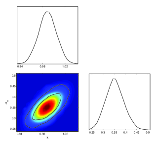
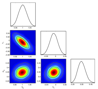
Figure 3: Normalized posterior likelihood of $\Omega_{m}$ in the flat $\Lambda$CDM model, which is derived from multi-frequency P15 sample.

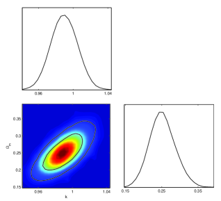
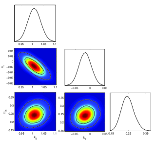
Figure 4: Cosmological constraints on the flat DGP model from multi-frequency P15 sample.

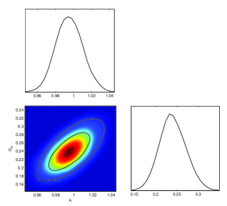
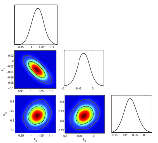
Figure 5: Normalized posterior likelihood of $\Omega_{m}$ in the flat $\Lambda$CDM model with Hubble constant from Riess (2016).

III Results and discussion

In order to demonstrate how the above described approach works we have constrained two simple cosmological models using the multi-frequency quasar data from Table 1. The models we chose are: the $\Lambda$CDM and Dvali-Gabadadze-Porrati (DGP) models under assumption of spatially flat Universe. In our fits the parameter $k$ representing the dependence of the angular size on frequency and its evolution with redshift are fitted together with cosmological parameters.

In our analysis we assumed flatness of the FRW metric, which is strongly indicated by the location of the first acoustic peak in the CMBR (Ade et al., 2014). This conclusion is also independently supported by the quasar data at $z\sim 3.0$ as demonstrated in (Cao et al., 2017b). It is a well known fact for the $\Lambda$CDM model while the DGP model requires a few words of reminder. This model is one of the simplest modified gravity models based on the concept of braneworld theory (Dvali00), in which gravity leaks out into the bulk above a certain cosmological scale $r_{c}$. Hence this scale is a free parameter of the theory which in the flat DGP model can be associated with the density parameter: $\Omega_{r_{c}}=1/(4r^{2}_{c}H^{2}_{0})$. It is then easy to see that the relation $\Omega_{r_{c}}=\frac{1}{4}(1-\Omega_{m})^{2}$ is valid. The results for different cosmological scenarios on the multi-frequency VLBI observations are listed in Table 1 and discussed in turn in the following sub-sections. The marginalized probability distribution of each parameter and the marginalized 2D confidence contours are presented in Fig. 3-6. In addition, we add the prior for the Hubble constant $H_{0}=67.3$ km $\rm s^{-1}$ $\rm Mpc^{-1}$ based on the recent Planck observations (Ade et al., 2014).

We started our analysis with the $\Lambda$CDM model with constant dark energy density and constant cosmic equation of state $w=p/\rho=-1$, while two cases of conical jet model were considered: a non-evolving constant $k$ parameter and an evolving one (denoted in Table 2 as $\Lambda$CDM1 and $\Lambda$CDM2, respectively). Parameters $k$, $k_{0}$ and $k_{1}$ were treated as free parameters to be fitted.

Firstly, based on the prior for the Hubble constant after Planck Collaboration XVI (2014), the likelihood is maximized at $\Omega_{m}=0.353\pm 0.063$ and $k=0.988\pm 0.025$ with multi-frequency measurements. In the second case, when the $k$ parameter representing the dependence of the angular size on frequency is allowed to evolve: $k(z)=k_{0}+k_{1}z$, treating intermediate luminosity quasars as standard rulers, whose intrinsic length determined at 2 GHz scales as $l_{m}\propto\nu^{-k}$ to any other frequency, the best-fit values for the parameters are $\Omega_{m}=0.348\pm 0.063$ and $k_{0}=0.999\pm 0.043$, and $k_{1}=-0.009\pm 0.0321$. The results are illustrated in Fig. 3. One can easily see that multi-frequency VLBI observations lead to reasonable cosmological fits, which motivates us to improve constraints with a larger quasar sample from future VLBI observations based on better uv-coverage. These results are illustrated in Fig. 3 and Table 2. For comparison, one should refer to recent results obtained with other independent precise measurements. First of all, the best fit value of matter density parameter in the framework of flat $\Lambda$CDM model reported by the Planck collaboration (Ade et al., 2014) was ${\Omega_{m}}=0.315\pm 0.017$. Then, Hinshaw et al. (2013) gave the best-fit parameter $\Omega_{m}=0.279$ for the flat $\Lambda$CDM model from the WMAP 9-year results, while the Hubble constant was constrained by them at $H_{0}=70.0\pm 2.2$ km $\rm s^{-1}$ $\rm Mpc^{-1}$. One can see that our results are consistent with these estimates. One can consider it as a consistency between the same type of probes – standard rulers – acoustic peaks revealed by CMBR anisotropy measurements at the redshift of $z\sim 1000$ and our quasar sample reaching the redshift of $z\sim 3.0$. One can see that $k$ parameter obtained from the multi-frequency sample is consistent with the Blandford & Königl (1979) conical jet model ($k=1$) at 1$\sigma$ confidence level. Fits on the $k$ parameter also reveal compatibility between our sample of quasars and the recent multi-frequency core shift measurements of many compact radio sources: Quasar 3C 345 (Lobanov, 1998) with extensive long-term VLBI monitoring database at four frequencies (5, 8.4, 10.6, 22.2 GHz); Quasar 0850+581 (Kovalev et al., 2008) with a dedicated VLBA experiment at 5, 8, 15, 24, and 43 GHz; Quasar 3C 309.1 and BL Lac object 0716+714 (Kovalev et al., 2009) observed with VLBA at four frequencies (8.1, 8.4, 12.1, 15.4 GHz); Blazar 1418+546, 2007+777, and 2200+420 (O’Sullivan & Gabuzda, 2009) observed with VLBA at eight frequencies (4.6, 5.1, 7.9, 8.9, 12.9, 15.4, 22.2, 43.1 GHz).

Concerning the DGP model, marginalized distribution of the model parameters are shown in Fig. 4. Considering the case that both $\Omega_{m}$ and $k$ are free parameters (denoted in Table 2 as DGP1), we get the marginalized 1$\sigma$ constraints of the parameters $\Omega_{m}=0.252\pm 0.055$ and $k=0.989\pm 0.024$. Working on the evolving $k$ parameter representing the dependence of the angular size on frequency, we find that the mass density parameter in DGP model ($\Omega_{m}=0.245\pm 0.054$) agrees very well with the respective value derived from joint analysis of standard rulers and standard candles including the measurements of the baryon acoustic oscillation (BAO), cosmic microwave background (CMB), strong gravitational lensing (SGL) and Type Ia supernovae (SNe Ia): ${\Omega_{m}}=0.267\pm 0.013$ (Biesiada et al., 2011). Constraints on the redshift-evolving $k$ parameters ($k_{0}=1.009\pm 0.043$, $k_{1}=-0.016\pm 0.032$) are even more consistent with the Blandford & Königl (1979) conical jet model and previous analysis especially with multi-frequency core shift measurements.

Finally, in the previous analysis we have assumed the prior for the Hubble constant after Planck Collaboration XVI (2014), a local determination of $H_{0}=73.24\pm 1.74$ km $\rm s^{-1}$ $\rm Mpc^{-1}$ with $2.4\%$ uncertainty from Riess et al. (2016) can be taken to perform consistency test. Such choice enables us to see the influence of the Hubble constant on the constraining power of our multi-frequency quasar data. Note that the Hubble constant derived from the GP-processed $H(z)$ measurements in our analysis, $H_{0}=69.2\pm 3.7$ km $\rm s^{-1}$ $\rm Mpc^{-1}$, is well consistent with the above three priors on $H_{0}$ at 68.3% confidence level. Such consistency has been extensively discussed in many previous works focusing on improved constraints on the Hubble constant through different model-independent methods (Li et al., 2016; Wang & Meng, 2016). Here, we estimate the constraint results of the flat $\Lambda$CDM with constant and evolving $k$ parameter, which are specifically shown in Fig. 5 and Table 2. It is obvious that the values of matter density obtained with the prior on $H_{0}$ taken after Riess et al. (2016), $\Omega_{m}=0.239\pm 0.047$ (with $k_{=}0.995\pm 0.023$) and $\Omega_{m}=0.229\pm 0.050$ (with $k_{0}=1.030\pm 0.042$, $k_{1}=-0.031\pm 0.032$), are generally lower than that given by most of other types of cosmological observations. This illustrates the importance of measuring the Hubble constant accurately with independent techniques and better understanding the nature of discrepancy between $H_{0}$ inferred from CMBR or BAO and from local measurements based on cosmic distance ladder. Summarizing, although the cosmological constraints become much weaker with the inclusion of different systematics, the current standard cosmological model ($\Omega_{m}\sim 0.3$) with a significant cosmological constant ($\Omega_{\Lambda}\sim 0.7$) in the flat universe is still preferred by our quasar sample at high confidence level.

IV Conclusions

In conclusion, our analysis demonstrates that multi-frequency angular size measurements of intermediate-luminosity quasars reaching the redshifts $z\sim 3$ can be used as standard rulers for cosmological inference. Therefore, one may say that the approach initiated in Cao et al. (2017a, b) can be further developed. More importantly, our results indicate that, the multi-frequency quasar sample is consistent with the Blandford & Königl (1979) conical jet model ($k=1$), which, from the physical point of view means that opacity of the jet is governed by pure synchrotron self-absorption, i.e. external absorption does not play any significant role in the observed angular sizes at least up to 43 GHz. One should stress that the present paper is only the first step toward elaborating the scheme to identify and calibrate compact radio-sources as standard rulers taking advantage of multi-frequency observations. Still, there are several remarks that remain to be clarified as follows.

Firstly, in performing the statistical analysis from the multi-frequency quasar data, we find that a precise determination of the linear size through a cosmological model-independent method plays an significant part to achieve such goal, which remains to be addressed in future analyses on a larger sample. On the one hand, we demonstrated that the approach initiated in Cao et al. (2017b), i.e., calibrating intermediate luminosity milliarcseconds compact radio quasars in sufficiently big sample obtained even at a single frequency is promising. Namely, the intrinsic metric size $l_{m}$ identified at some observing frequency, when properly rescaled, can be used in objects observed in other surveys performed at other frequencies. On the other hand, although the cosmological constraints derived from multi-frequency data in the current study agrees very well with that form the previous sample based on single-frequency data, this inference still heavily relies on the assumption of Blandford & Königl (1979) conical jet model, i.e., the radio core tends to be self-absorbed and in equipartition. Moreover, it is of paramount importance to determine precisely to which extent this holds for the intermediate luminosity quasars, which should be done in the future on a much larger sample.

Secondly, there are several sources of systematics we do not consider in this paper and which remain to be addressed in the future analysis. Let us start with the possible biases associated with sample incompleteness. One general concern is given by the fact that there are different ranges of frequencies addressed for each source in the compiled data by Pushkarev & Kovalev (2015). Although this problem has been recognized long time ago, the most straightforward solution to this issue is focusing on a larger sample of multi-frequency measurements of compact structure covering the same range of frequencies, which is hard to be rigorously accounted in context of cosmological studies like in this paper. The other systematic is the scattering in the size determination of objects at cosmological distances, which would furthermore affect the derived value of the $k$ parameter. More specifically, if the intergalactic medium broadens the signal of the radio sources, the apparent size will be larger at larger distances (Gurvits, 1994; Gurvits, Kellerman & Frey, 1999). Further progress has recently been achieved in the study of Milky Way scattering properties and intrinsic sizes of active galactic nuclei cores (Pushkarev & Kovalev, 2015). The so-called Galactic broadening is found to be dependent on the galactic latitude and intrinsic scattering, while its strength is possibly correlated with the Galactic H$\alpha$ intensity, free-electron density, and Galactic rotation measurements. However, one should note that such effect is still difficult to be precisely quantified, especially in the case when the Universe is filled with charged particles.

Thirdly, even with a relatively small sample of 30 sources we were able to demonstrate that combined multi-frequency data concerning compact radio quasars gives quite stringent cosmographic constraints and is able to differentiate between different cosmological models like $\Lambda$CDM and DGP. The value of density parameter in $\Lambda$CDM model is perfectly consistent with values obtained in an independent manner. Moreover when confronted with alternative methods of determining $\Omega_{m}$ like from the peculiar velocities of galaxies Feldman et al. (2003) our fits obtained for the DGP model are accurate enough to falsify this model. However, strong degeneracy between $H_{0}$ and $\Omega_{m}$, illustrated in our study in the spirit of sensitivity analysis, emphasizes the importance of independent and more direct determinations of $H_{0}$. In this respect the approach of strong lensing time delays is promising. Recent results of the H0LiCOW project (Bonvin et al., 2017) already demonstrated that a few percent accuracy in $H_{0}$ determination is feasible.

Finally, the results presented in this paper pave the way for the follow up engaging multi-frequency VLBI observations of more compact radio quasars with higher sensitivity and angular resolution, which may make it less susceptible to systematic errors. The approach, introduced in this paper, would make it possible to build a significantly larger sample of standard rulers at much higher redshifts. With such a sample, we can further investigate constraints on the cosmic evolution and eventually probe the evidence for dynamical dark energy (Wei & Wu, 2016; Cao et al., 2017c).

References

- Buchalter et al. (1998) Buchalter, A., Helfand, D. J., Becker, R. H., & White, R. L., 1998, ApJ, 494, 503
- Guerra & Daly (1998) Guerra, E. J., & Daly, R. A. 1998, ApJ, 493, 536
- Guerra, Daly & Wan (2000) Guerra, E. J., Daly, R. A., & Wan, L. 2000, ApJ, 544, 659
- Daly & Djorgovski (2003) Daly, R. A., & Djorgovski, S. G. 2003, ApJ, 597, 9
- Kellermann (1993) Kellermann, K. I. 1993, Nature, 361, 134
- Gurvits (1994) Gurvits, L. I., 1994, ApJ, 425, 442
- Amanullah et al. (2010) Amanullah, R., et al. 2010, ApJ, 716, 712
- Gurvits, Kellerman & Frey (1999) Gurvits, L. I., Kellerman, K. I., & Frey, S. 1999, A&A, 342, 378
- Vishwakarma (2001) Vishwakarma, R. G. 2001, Classical Quantum Gravity, 18, 1159
- Zhu & Fujimoto (2002) Zhu, Z.-H., & Fujimoto, M. K. 2002, ApJ, 581, 16
- Chen & Ratra (2003) Chen, G., & Ratra, B. 2003, ApJ, 582, 58
- Cao et al. (2015) Cao, S., Biesiada, M., Zheng, X. & Zhu, Z.-H. 2015, ApJ, 806, 66
- Cao et al. (2017a) Cao, S., Biesiada, M., Jackson, J., Zheng, X. & Zhu Z.-H. 2017a, JCAP, 02, 012
- Cao et al. (2017b) Cao, S., Zheng X., Biesiada M., Qi J., Chen Y. & Zhu Z.-H. 2017b, A&A, 606, A15
- Li et al. (2017) Li, X. L., Cao, S., Zheng, X., Qi, J. Z., Biesiada, M., & Zhu, Z.-H. 2017, EPJC, 77, 677
- Zheng et al. (2017) Zheng, X., Biesiada, M., Cao, S., Qi, J. Z., & Zhu, Z.-H. 2017, JCAP, 10, 030
- Qi et al. (2017) Qi, J. Z., Cao, S., Biesiada, M., Zheng, X. & Zhu, Z.-H. 2017, EPJC, 77, 502
- Xu et al. (2017) Xu, T. P., Cao, S., Qi, J. Z., Biesiada, M., Zheng, X. & Zhu, Z.-H. 2017, JCAP, submitted [arXiv:1708.08631]
- Lobanov (1998) Lobanov, A. P. 1998, A&A, 330, 79
- Blandford & Königl (1979) Blandford, R. D., & Königl, A., 1979, ApJ, 232, 34
- Sandage (1988) Sandage, A. 1988, ARA&A, 26, 561
- Blandford & Rees (1978) Blandford, R. D. & Rees, M. J. 1978, “Some comments on radiation mechanisms in Lacertids, in BL Lac Objects” (ed. A.M.Wolfe), University of Pittsburgh, Pittsburgh, pp. 328-341
- Marscher & Shaffer (1980) Marscher A. P., & Shaffer D. B. 1980, AJ, 85, 668
- O’Sullivan & Gabuzda (2009) O’Sullivan, S. P., & Gabuzda, D. C. 2009, MNRAS, 393, 429
- Antonucci (1993) Antonucci, R. 1993, ARA&A, 31, 473
- Antonucci (2015) Antonucci, R. 2015, arXiv:1501.02001
- Wilkinson et al. (1994) Wilkinson, P. N., et al. 1994, ApJ, 432, L87
- Pushkarev & Kovalev (2012) Pushkarev, A. B., & Kovalev, Y. Y. 2012, A&A, 544, 34
- Dabrowski et al. (1995) Dabrowski, Y., Lasenby A., & Saunders R. 1995, MNRAS, 277, 753
- Jackson (2004) Jackson, J. C. 2004, JCAP, 11, 7
- Pushkarev & Kovalev (2015) Pushkarev, A. B., & Kovalev, Y. Y. 2015, MNRAS, 452, 4274
- Hutter & Mufson (1986) Hutter, D. J. & Mufson, S. L. 1986, ApJ, 301, 50
- Bloom & Marscher (1996) Bloom, S. D. & Marscher, A. P. 1996, ApJ, 461, 657
- Kovalev et al. (2008) Kovalev, Y. Y., et al. 2008, Mem.S.A.It. 79, 1153
- Kovalev et al. (2009) Kovalev, Y. Y., et al. 2009, arXiv:0904.2458
- Preston et al. (1985) Preston, R. A., Morabito D. D., Williams J. G., Faulkner J., Jauncey D. L., Nicolson G. D., 1985, AJ, 90, 1599
- Moresco et al. (2012) Moresco, M., et al. 2012, JCAP, 1208, 006
- Zheng et al. (2016) Zheng, X., Ding, X., Biesiada, M., Cao, S., & Zhu, Z.-H. 2016, ApJ, 825, 1
- Jimenez & Loeb (2002) Jimenez, R. & Loeb, A., 2002, ApJ, 573, 37
- Seikel et al. (2012) Seikel, M., Clarkson, C., & Smith, M. 2012, JCAP, 6, 36
- Roukema et al. (2015) Roukema, B., Buchert, T., Ostrowski, J. J. & France, M. J. 2015, MNRAS, 448, 1660
- Roukema et al. (2016) Roukema, B., Buchert, T., Fuji, H. & Ostrowski J. J. 2016, MNRAS, 456, L45
- De Filippis et al. (2005) De Filippis, E., SerenoM, M., Bautz, W., Longo, G. 2005, ApJ, 625, 108
- Bonamente et al. (2006) Bonamente, M., et al. 2006, ApJ, 647, 25
- Jackson & Jannetta (2006) Jackson J. C., Jannetta A.L., 2006, JCAP, 11, 002
- Kovalev et al. (2005) Kovalev, Y. Y., et al. 2005, AJ, 130, 2473
- Ade et al. (2014) Ade, P. A. R., et al. 2014, A&A, 571, A16
- Hinshaw et al. (2013) Hinshaw, G., et al. 2013, ApJS, 208, 19
- Biesiada et al. (2011) Biesiada, M., et al. 2011, RAA, 11, 641
- Riess et al. (2016) Riess, A. G., Macri, L. M., Hoffmann, S. L., et al. 2016, ApJ, 826, 56
- Li et al. (2016) Li, Z. X., et al. 2016, PRD, 93, 043014
- Wang & Meng (2016) Wang, D., & Meng, X. H. 2016, arXiv:1610.01202v1
- Feldman et al. (2003) Feldman, H. A., et al. 2003, ApJL, 596, L131
- Bonvin et al. (2017) Bonvin,V., et al. 2017, MNRAS, 465, 4914
- Wei & Wu (2016) Wei, J. J. & Wu, X. F. 2016, arXiv:1611.00904v1
- Cao et al. (2017c) Cao, S., et al. 2017c, arXiv:1708.08608