The completeness-corrected rate of stellar encounters with the Sun from the first Gaia data release

I report on close encounters of stars to the Sun found in the first Gaia data release (GDR1). Combining Gaia astrometry with radial velocities of around 320 000 stars drawn from various catalogues, I integrate orbits in a Galactic potential to identify those stars which pass within a few parsecs. Such encounters could influence the solar system, for example through gravitational perturbations of the Oort cloud. 16 stars are found to come within 2 pc (although a few of these have dubious data). This is fewer than were found in a similar study based on Hipparcos data, even though the present study has many more candidates. This is partly because I reject stars with large radial velocity uncertainties ($>$10 km s^-1), and partly because of missing stars in GDR1 (especially at the bright end). The closest encounter found is Gl 710, a K dwarf long-known to come close to the Sun in about 1.3 Myr. The Gaia astrometry predict a much closer passage than pre-Gaia estimates, however: just 16 000 AU (90% confidence interval: 10 000–21 000 AU), which will bring this star well within the Oort cloud. Using a simple model for the spatial, velocity, and luminosity distributions of stars, together with an approximation of the observational selection function, I model the incompleteness of this Gaia-based search as a function of the time and distance of closest approach. Applying this to a subset of the observed encounters (excluding duplicates and stars with implausibly large velocities), I estimate the rate of stellar encounters within 5 pc averaged over the past and future 5 Myr to be $545\pm 59$ Myr^-1. Assuming a quadratic scaling of the rate within some encounter distance (which my model predicts), this corresponds to $87\pm 9$ Myr^-1 within 2 pc. A more accurate analysis and assessment will be possible with future Gaia data releases.

1 Introduction

What influence has the Galactic environment had on the solar system? How has this environment changed with time? As the solar system moves through the Galaxy, it is likely to come close to other stars. Ionizing radiation from particularly hot or active stars could adversely affect life on Earth. Tidal forces could shear the Oort cloud, the postulated body of primordial comets orbiting in the cold, dark outskirts of the solar system. This could push some bodies into the inner solar system in the form of comet showers, where they could potentially impact the Earth.

Reconstructing the encounter history (and future) of the solar system is possible by observing the present day positions and velocities of stars, and tracing their paths back and forward in time. Such studies came into their own after 1997 with the publication of the Hipparcos catalogue, which lists the positions, proper motions, and parallaxes of some 120 000 stars. The various studies performed before and since Hipparcos have identified tens of stars which have – or which will – come within 2 pc of the Sun (Matthews, 1994; Mülläri & Orlov, 1996; García-Sánchez et al., 1999, 2001; Dybczyński, 2006; Bobylev, 2010a, b; Jiménez-Torres et al., 2011; Bailer-Jones, 2015a; Dybczyński & Berski, 2015; Mamajek et al., 2015; Berski & Dybczyński, 2016). One of these articles, Bailer-Jones (2015a) (hereafter paper 1), is the precursor to the present work, and was based on the Hipparcos-2 catalogue (van Leeuwen, 2007) combined with various radial velocity catalogues. Dybczyński & Berski (2015) looked more closely at some of the encounters discovered in paper 1, in particular those flagged as problematic.

The closer a stellar encounter, the larger the tidal force on the Oort cloud. But the ability to perturb the orbit of a comet depends also on the mass and relative speed of the encounter. This can be quantified using an impulse approximation (Öpik, 1932; Oort, 1950; Rickman, 1976; Dybczynski, 1994). One version of this (Rickman, 1976) says the change in velocity of an Oort cloud comet due to a star of mass $M$ passing a distance $d_{\rm ph}$ at speed $\mathrm{v}_{\rm ph}$ is proportional to

$$\frac{M}{\mathrm{v}_{\rm ph}\,d_{\rm ph}^{2}}\ .$$ (1)

For the much rarer, very close approaches (on the order of the comet–Sun separation), the dependence on distance is more like $1/d_{\rm ph}$ (see Feng & Bailer-Jones (2015) for some empirical comparison). More sophisticated modelling of the effect of passing stars on the Oort cloud has been carried out by, for example, Scholl et al. (1982); Weissman (1996); Dybczyński (2002); Fouchard et al. (2011); Rickman et al. (2012). Feng & Bailer-Jones (2015) looked specifically at the consequence of the closest encounters found in paper 1.

Our ability to find and characterize close encounters has received a huge boost by the launch of the Gaia astrometric satellite in December 2013 (Gaia Collaboration et al., 2016b). This deep, accurate astrometric survey will eventually provide positions, parallaxes, and proper motions for around a billion stars, and radial velocities for tens of millions of them. The first Gaia data release (GDR1) in September 2016 (Gaia Collaboration et al., 2016a), although based on a short segment of data and with only preliminary calibrations, included astrometry for two million Tycho sources (Høg et al., 2000) down to about 13th magnitude, with parallaxes and proper motions a few times more accurate than Hipparcos (Lindegren et al., 2016). This part of GDR1 is known as the Tycho-Gaia Astrometric Solution (TGAS), as it used the Tycho coordinates from epoch J1991.25 to lift the degeneracy between parallax and proper motion which otherwise would have occurred when using a short segment of Gaia data.

The first goal of this paper is to find encounters from combining TGAS with various radial velocity catalogues. The method, summarized in section 2 is very similar to that described in paper 1. One important difference here is the exclusion of stars with large radial velocity uncertainties. I search for encounters out to 10 pc, but really we are only interested in encounters which come within about 2 pc. More distant encounters would have to be very massive and slow to significantly perturb the Oort cloud. The encounters are presented and discussed in section 3.

The other goal of this paper is to model the completeness in the perihelion time and distance of searches for close encounters. This involves modelling the spatial, kinematic, and luminosity distribution of stars in the Galaxy, and combining these with the survey selection function to construct a two-dimensional completeness function. A simple model is introduced and its consequences explored in section 4. Using this model I convert the number of encounters detected into a prediction of the intrinsic encounter rate out to some perihelion distance. This study is a precursor to developing a more sophisticated incompleteness-correction for subsequent Gaia data releases, for which the selection function should be better defined.

The symbols $t_{\rm ph}$, $d_{\rm ph}$, and $\mathrm{v}_{\rm ph}$ indicate the perihelion time, distance, and speed respectively (“ph” stands for perihelion). The superscript “lin” added to these refers to the quantity as found by the linear motion approximation of the nominal data (where “nominal data” means the catalogue values, rather than resamplings thereof). The superscript “med” indicates the median of the distribution over a perihelion parameter found by orbit integration (explained later). Preliminary results of this work were reported at the Nice IAU symposium in April 2017 (Bailer-Jones, 2017).

2 Procedure for finding close encounters

The method is similar to that described in paper 1, but differs in part because the radial velocity (RV) catalogue was prepared in advance of the Gaia data release.

1. I searched CDS/Vizier in early 2016 for RV catalogues which had a magnitude overlap with Tycho-2 and a typical radial velocity precision, $\sigma(\mathrm{v}_{r})$, better than a few km s^-1. I ignored catalogues of stellar cluster members, those obsoleted by later catalogues, or those with fewer than 200 entries. Where necessary, I cross-matched them with Tycho-2 using the CDS X-match service to assign Tycho-2 IDs (or Hipparcos IDs for those few Hipparcos stars which do not have Tycho-2 IDs). The union of all these catalogues I call RVcat. A given star may appear in more than one RV catalogue or more than once in a given catalogue, so RVcat contains duplicate stars. Each unique entry in RVcat I refer to as an object. RVcat contains 412 742 objects.

   Missing $\sigma(\mathrm{v}_{r})$ values were replaced with the median of all the other values of $\sigma(\mathrm{v}_{r})$ in that catalogue. Malaroda2012 lists no uncertainties, so I somewhat arbitrarily set them to 0.5 km s^-1. For APOGEE2 I took the larger of its catalogue entries RVscatter and RVerrMed and added 0.2 km s^-1 in quadrature, following the advice of Friedrich Anders (private communication). For Galah I conservatively use 0.6 km s^-1, following the statement in Martell et al. (2017) that 98% of all stars have a smaller standard deviation than this.

2. I then independently queried the Gaia-TGAS archive to find all stars which, assuming them all to have radial velocities of $|\mathrm{v}_{r}|=750$ km s^-1, would come within 10 pc of the Sun according to the linear motion approximation (LMA) ($d_{\rm ph}^{\rm lin}<10$ pc). The LMA models stars as moving on unaccelerated paths relative to the Sun, so has a quick analytic solution (see paper 1). By using a fixed radial velocity I could run the archive query (listed in appendix A) independently of any RV catalogue, and by using the largest plausible radial velocity I obtained the most-inclusive list of encounters (the larger the radial velocity, the closer the approach). The value of 750 km s^-1 is chosen on the basis that the escape velocity from the Galaxy (with the model adopted for the orbit integrations) is 621 km s^-1 at the Galactic Centre (GC) and 406 km s^-1 at the solar circle; a reasonable upper limit is 500 km s^-1. To this I add the velocity of the Sun relative to the GC (241 km s^-1) to set a limit of 750 km s^-1, on the assumption that very few stars are really escaping from the Galaxy. This query (run on 16-11-2016) identified 541 189 stars. Stars with non-positive parallaxes are removed, leaving 540 883 stars (call this ASTcat).

3. I now remove from RVcat all objects which have $|\mathrm{v}_{r}|>750$ km s^-1 or $\sigma(\mathrm{v}_{r})>10$ km s^-1 or which have one of these values missing. This reduces RVcat to 397 788 objects, which corresponds to 322 462 unique stars. This is approximately the number of objects/stars I can test for being encounters. The number of objects for each of the catalogues is shown in column 3 of Table 1.

   Table 1: The number of objects (not unique stars) in the RV catalogues. The first column gives the catalogue reference number (used in Table 3) and the second column a reference name. The third column lists the number of objects with valid Tycho/Hipparcos IDs which also have $|\mathrm{v}_{r}|\leq 750$ km s^-1 and $\sigma(\mathrm{v}_{r})\leq 10$ km s^-1. This is approximately the number of objects available for searching for encounters. The fourth column lists how many of these have $d_{\rm ph}^{\rm lin}<10$ pc. There are duplicate stars between (and even within) the catalogues.

   cat	name	#Tycho	#($d_{\rm ph}^{\rm lin}<10$ pc)
   1	RAVE-DR5	302 371	240
   2	GCS2011	13 548	157
   3	Pulkovo	35 745	238
   4	Famaey2005	6 047	1
   5	Web1995	429	5
   6	BB2000	670	5
   7	Malaroda2012	1 987	12
   8	Maldonado2010	349	32
   9	Duflot1997	43	0
   10	APOGEE2	25 760	33
   11	Gaia-ESO-DR2	159	0
   12	Galah	10 680	2
   Total		397 788	725

   Notes: References and (where used) CDS catalogue numbers for the RV catalogues: (1) Kunder et al. (2017); (2) Casagrande et al. (2011) J/A+A/530/A138/catalog; (3) Gontcharov (2006) III/252/table8; (4) Famaey et al. (2005) J/A+A/430/165/tablea1; (5) Duflot et al. (1995) III/190B; (6) Barbier-Brossat & Figon (2000) III/213; (7) Malaroda et al. (2000) III/249/catalog; (8) Maldonado et al. (2010) J/A+A/521/A12/table1; (9) Fehrenbach et al. (1997) J/A+AS/124/255/table1; (10) SDSS Collaboration et al. (2016); (11) https://www.gaia-eso.eu; (12) Martell et al. (2017).

4. The common objects between this reduced RVcat and ASTcat are identified (using the Tycho/Hipparcos IDs). These 98 849 objects all have – by construction – a Tycho/Hipparcos ID, TGAS data, positive parallaxes, $|\mathrm{v}_{r}|\leq 750$ km s^-1, $\sigma(\mathrm{v}_{r})\leq 10$ km s^-1, and would encounter the Sun within 10 pc (using the LMA) if they had a radial velocity of 750 km s^-1. Applying the LMA now with the measured radial velocity, I find that 725 have $d_{\rm ph}^{\rm lin}<10$ pc. The number per RV catalogue is shown in the fourth column of Table 1. Only these objects will be considered in the rest of this paper. The distribution of the measurements, including their standard deviations and correlations, can be found in Bailer-Jones (2017).

5. These 725 objects are then subject to the orbit integration procedure described in sections 3.3 and 3.4 of paper 1. This gives accurate perihelia both by modelling the acceleration of the orbit and by numerically propagating the uncertainties through the nonlinear transformation of the astrometry. To summarize: the 6D Gaussian distribution of the data (astrometry plus radial velocity) for each object is resampled to produce 2000 “surrogate” measurements of the object. These surrogates reflect the uncertainties in the position and velocity (and takes into account their covariances, which can be very large). The orbit for every surrogate is integrated through the Galactic potential and the perihelia found. The resulting distribution of the surrogates over the perihelion parameters represents the propagated uncertainty. These distributions are asymmetric; ignoring this can be fatal (see section 3.1 for an example). I summarize the distributions using the median and the 5% and 95% percentiles (which together form an asymmetric 90% confidence interval, CI). I use the same Galactic model as in paper 1. The integration scheme is also the same, except that I now recompute the sampling times for each surrogate, as this gives a better sampling of the orbit.

This procedure does not find all encounters, because an initial LMA-selection is not guaranteed to include all objects which, when properly integrated, would come within 10 pc. Yet as the LMA turns out to be a reasonable approximation for most stars (see next section), this approach is adequate for identifying encounters which come much closer than 10 pc.

3 Close encounters found in TGAS

As duplicates are present in the RV catalogue, the 725 objects found correspond to 468 unique stars (unique Tycho/Hipparcos IDs). The numbers coming within various perihelion distances are shown in Table 2. The data for those with $d_{\rm ph}^{\rm med}<2$ pc are shown in Table 3 (the online table at CDS includes all objects with $d_{\rm ph}^{\rm med}<10$ pc). Negative times indicate past encounters.

Table 2: The number of objects and stars found by the orbit integration to have $d_{\rm ph}^{\rm med}<d_{\rm ph}^{\rm max}$. An object is a specific catalogue entry for a star. Objects with potentially problematic data have not been excluded.

$d_{\rm ph}^{\rm max}$	No. objects	No. stars
$\infty$	725	468
$10$	646	402
$5$	149	97
$3$	56	42
$2$	20	16
$1$	2	2
$0.5$	1	1

Table 3: Perihelion parameters for all objects with a median perihelion distance (median of the samples; $d_{\rm ph}^{\rm med}$) below 2 pc, sorted by this value. The first column list the Tycho ID. The second column indicates the RV catalogue (see Table 1). Columns 3, 6, and 9 are $t_{\rm ph}^{\rm med}$, $d_{\rm ph}^{\rm med}$, and $\mathrm{v}_{\rm ph}^{\rm med}$ respectively. The columns labelled 5% and 95% are the bounds of corresponding confidence intervals. Columns 12–14 (“% samples”) indicate the percentage of surrogates for each object for which $d_{\rm ph}$ is below 0.5, 1.0, and 2.0 pc respectively. Columns 15–20 list the nominal parallax ($\varpi$), proper motion ($\mu$), and radial velocity ($\mathrm{v}_{r}$) along with their standard errors. Objects with potentially problematic data have not been excluded. The online table at CDS includes all objects with $d_{\rm ph}^{\rm med}<$10 pc (in a handful of cases for $d_{\rm ph}^{\rm med}>2$ pc the ID is Hipparcos, not Tycho).

1	2	3	4	5	6	7	8	9	10	11	12	13	14	15	16	17	18	19	20
ID		$t_{\rm ph}$ / kyr			$d_{\rm ph}$ / pc			$\mathrm{v}_{\rm ph}$ / km s-1			% samples			$\varpi$	$\sigma(\varpi)$	$\mu$	$\sigma(\mu)$	$\mathrm{v}_{r}$	$\sigma(\mathrm{v}_{r})$
		med	5%	95%	med	5%	95%	med	5%	95%	0.5	1	2	mas		mas yr-1		km s-1
5102-100-1	3	1354	1304	1408	0.08	0.05	0.10	13.8	13.3	14.3	100	100	100	52.35	0.27	0.50	0.17	-13.8	0.3
4744-1394-1	1	-1821	-2018	-1655	0.87	0.61	1.20	121.0	118.6	123.6	1	74	100	4.44	0.26	0.59	0.12	120.7	1.6
1041-996-1	3	3386	3163	3644	1.26	1.07	1.50	30.4	29.9	30.9	0	1	100	9.51	0.41	0.57	0.05	-30.4	0.3
5033-879-1	1	-704	-837	-612	1.28	0.48	2.63	532.7	522.7	543.2	6	30	83	2.60	0.25	0.91	0.78	532.4	6.2
709-63-1	3	-497	-505	-490	1.56	1.53	1.59	22.2	21.9	22.5	0	0	100	87.66	0.29	56.44	0.09	22.0	0.2
4753-1892-2	3	-948	-988	-910	1.58	1.46	1.72	55.0	54.5	55.5	0	0	100	18.75	0.47	6.52	0.05	55.0	0.3
4753-1892-1	3	-949	-990	-908	1.59	1.46	1.73	55.0	54.5	55.5	0	0	100	18.75	0.47	6.52	0.05	55.0	0.3
4753-1892-2	2	-970	-1027	-921	1.62	1.49	1.78	53.7	51.6	55.9	0	0	99	18.75	0.47	6.52	0.05	53.7	1.3
4753-1892-1	2	-971	-1028	-915	1.63	1.48	1.78	53.8	51.5	55.9	0	0	100	18.75	0.47	6.52	0.05	53.7	1.3
4855-266-1	3	-2222	-2297	-2153	1.67	1.51	1.84	34.6	34.1	35.1	0	0	99	12.74	0.24	1.68	0.13	34.5	0.3
8560-8-1	1	-634	-656	-614	1.72	1.25	2.26	86.5	85.4	87.4	0	0	80	17.84	0.33	9.79	1.78	86.4	0.6
6510-1219-1	3	-1951	-2021	-1880	1.74	1.66	1.81	14.6	14.2	15.1	0	0	100	34.19	0.29	6.29	0.04	14.6	0.3
5383-187-1	10	-870	-1324	-651	1.74	0.40	6.23	686.8	683.2	690.1	7	24	56	1.63	0.36	0.55	0.57	686.7	2.1
6510-1219-1	2	-1975	-2028	-1924	1.76	1.69	1.82	14.5	14.1	14.8	0	0	100	34.19	0.29	6.29	0.04	14.4	0.2
1315-1871-1	3	-651	-663	-640	1.78	1.72	1.84	40.6	40.4	40.7	0	0	100	36.93	0.40	21.13	0.04	40.5	0.1
1315-1871-1	2	-651	-663	-640	1.78	1.72	1.84	40.6	40.4	40.7	0	0	100	36.93	0.40	21.13	0.04	40.5	0.1
6975-656-1	1	-457	-554	-390	1.80	0.89	3.89	563.1	547.2	578.3	0	9	58	3.79	0.39	2.76	1.72	562.9	9.2
4771-1201-1	3	-1848	-1917	-1783	1.89	1.70	2.09	22.2	21.6	22.9	0	0	82	23.79	0.33	4.96	0.03	22.2	0.4
9327-264-1	1	-1889	-2014	-1777	1.91	1.10	3.18	52.7	51.3	54.2	0	3	56	9.83	0.34	1.44	0.82	52.4	0.9
7068-802-1	1	-2641	-2857	-2455	1.99	0.54	4.59	65.5	62.6	68.4	4	17	50	5.67	0.23	0.76	0.66	65.0	1.8

Figure 1 plots the perihelion times and distances. Although the objects were selected by the LMA to come within 10 pc of the Sun, some of the orbit integrations result in much larger median perihelion distances. The differences between the two estimates – LMA and median of orbit-integrated surrogates – are shown in Figure 2. The differences arise both due to gravity and to the resampling of the data. The largest differences are seen at larger (absolute) times. These objects have small and low-significance parallaxes and proper motions. The resulting distribution over the perihelion parameters is therefore very broad (as seen from the large confidence intervals in Figure 1), with the consequence that the median can differ greatly from the LMA value. If I use the LMA to find the perihelion of the surrogates and then compute their median, there are still large differences compared to the orbit integration median (up to 170 pc; the plot of differences looks rather similar to Figure 2). This proves that the inclusion of gravity, and not just the resampling of the data, has a significant impact on the estimated perihelion parameters.

As we are only interested in encounters which come within a few pc, Figure 3 zooms in to the perihelion range 0–5 pc. The perihelion speeds for these objects are shown in Figure 4.

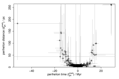
Figure 1: Perihelion times and distances computed by orbit integration for all 725 objects. Open circles show the median of the perihelion time and distance distributions. The error bars show the limits of the 5% and 95% percentiles (which together form an asymmetric 90% confidence interval). Note that this set of objects includes duplicates (see Table 2).

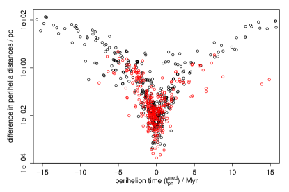
Figure 2: Difference between perihelion estimates from orbit integration of surrogates ($d_{\rm ph}^{\rm med}$) and the linear motion approximation ($d_{\rm ph}^{\rm lin}$), on a log scale. The black symbols are for $d_{\rm ph}^{\rm med}>d_{\rm ph}^{\rm lin}$, the red symbols for $d_{\rm ph}^{\rm med}<d_{\rm ph}^{\rm lin}$. The set of objects is the same as shown in Figure 1, but excluding, for plotting purposes, the three points with $|t_{\rm ph}^{\rm med}|>20$ Myr.

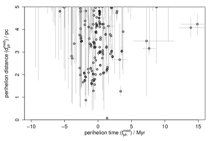
Figure 3: As Figure 1, but zoomed in to the range $0\leq d_{\rm ph}^{\rm med}\leq 5$. The time axis is scaled to show all encounters in this distance range.

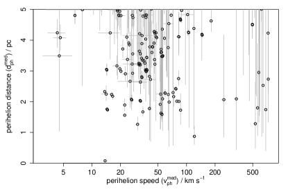
Figure 4: Median perihelion velocities from the orbit integrations for those encounters shown in Figure 3.

Immediately apparent in Figure 3 is the very close encounter at 1.3 Myr in the future. This is the K7 dwarf Gl 710 (Tyc 5102-100-1, Hip 89825), known from many previous studies to be a very close encounter. In paper 1 I found a median encounter distance of 0.26 pc (90% CI 0.10–0.44 pc). TGAS reveals a much smaller proper motion than Hipparcos-2: $0.50\pm 0.17$ mas yr^-1 as opposed to $1.8\pm 1.2$ mas yr^-1 (the parallax is the same to within 2%). Using the same radial velocity, my orbit integration now gives a median perihelion distance of 0.08 pc (90% CI 0.05–0.10 pc), equivalently 16 000 AU (90% CI 10 000–21 000 AU). This makes Gl 710 once again the closest known stellar encounter. Berski & Dybczyński (2016) found a very similar value using the same data and a similar method. Although this close approach will take Gl 710 well within the Oort cloud – and its relative velocity at encounter is low (14 km s^-1) – its low mass (around 0.6 M_⊙) limits its perturbing influence. This is analysed by Berski & Dybczyński (2016).

The second closest encounter is Tyc 4744-1394-1 at $d_{\rm ph}^{\rm med}$ = 0.87 pc, two million years ago. This is based on a RAVE radial velocity of $120.7\pm 1.6$ km s^-1. A second RAVE measurement gives $15.3\pm 1.2$ km s^-1, which puts the encounter at a much larger distance of $d_{\rm ph}^{\rm med}=36.6$ pc, 12.9 Myr in the past. This discrepancy may suggest both measurements are unreliable.

Tyc 1041-996-1 (Hip 94512) was found in paper 1 to encounter between 0.59–3.30 pc or 0.58–4.60 pc (90% CI), depending on the whether the Tycho-2 or Hipparcos-2 proper motion was adopted. TGAS puts a much tighter constraint on its perihelion distance, using the same radial velocity.

Tyc 5033-879-1 is not in Hipparcos so was not in paper 1, and has not previously been reported as a close encounter. Its large radial velocity is from RAVE (DR5). The spectrum has a very low SNR, and the standard deviation computed by resampling is very high (StdDev_HRV = 246 kms), so this measurement is probably spurious. This catalogue lists a second value of $-6.5\pm 7.0$ km s^-1 for the same RAVE ID (RAVE J160748.3-012060). Another object with a different RAVE ID (RAVE J160748.3-012059) – but very close by, and matched to the same Tycho ID by RAVE – has $-11.6\pm 2.1$ km s^-1.

Tyc 709-63-1 is Hip 26335. I found this to be a close encounter with very similar perihelion parameters in paper 1. The TGAS measurements are very similar to those from Hipparcos-2, but more precise.

I make no special provision for unresolved physical binaries in my search for encounters. The two objects Tyc 4753-1892-1 and Tyc 4753-1892-2 listed in Table 3 are in fact the two components of the spectroscopic binary Hip 25240, for which there is just one entry in TGAS (but both were listed separately in two RV catalogues). Their mutual centre-of-mass motion means the encounter parameters computed will be slightly in error. This could be corrected for in some known cases, but the many more cases of unidentified binarity would remain uncorrected. The situation will improve to some degree once Gaia includes higher order astrometric solutions for physical binaries (see section 6).

Many of the other objects found in this study were likewise found to be close encounters in paper 1, sometimes with different perihelion parameters. The main reasons why some were not found in the earlier study are: not in the Hipparcos catalogue (for example because they were too faint); no radial velocity available; the TGAS and Hipparcos astrometry differ so much that $d_{\rm ph}$ was too large using the Hipparcos data to be reported in paper 1.

A few of the other closest encounters in Table 3 have suspiciously high radial velocities. Some or all of these may be errors, although it must be appreciated that close encounters are generally those stars which have radial velocities much larger than their transverse velocities. Tyc 5383-187-1 is, according to Simbad, a B9e star. If the radial velocity from APOGEE (SDSS 2M06525305-1000270) is correct – and this is questionable – its perihelion speed was a whopping 687 km s^-1. As its proper motion is very uncertain ($0.55\pm 0.57$) mas yr^-1, the range of perihelion distances is huge. The radial velocity for Tyc 6975-656-1 is from RAVE. The value StdDev_HRV = 545 km s^-1 in that catalogue indicates its radial velocity, and therefore its perihelion parameters, are highly unreliable.

Slightly surprising is the fact that 18 of the 20 objects with $d_{\rm ph}^{\rm med}<2$ pc have encounters in the past. However, these 20 objects only correspond to 15 systems, and 13 of 15 is not so improbable. Moreover, for $d_{\rm ph}^{\rm med}<3$ pc the asymmetry is much weaker: 35 objects have encounters in the past vs 21 in the future.

Figure 5: Comparison of object encounters found in the present work with TGAS (left) and those found in paper 1 from Hipparcos (right). Both sets of estimates are from the linear motion approximation of the nominal data. In the left and right panels there are 16 objects and 1 object respectively which lie at times beyond the limits of the plots. Both panels shows all objects, not unique stars, so include duplicates.

Figure 5 compares the encounters found in paper 1 with those found in the present study. For this comparison I use the perihelion parameters computed by the LMA with the nominal data, as this permits an unbiased comparison out to 10 pc. The most striking feature is that the Hipparcos-based study finds more encounters (1704 vs. 725 objects; 813 vs. 468 stars), despite the fact that the number of objects searched for encounters (i.e. those with complete and appropriate astrometry and radial velocities) is nearly four times larger in the present study: 397 788 compared to 101 363. Looking more closely, we also see that the present study finds comparatively few encounters at perihelion times near to zero. This is partly due to the fact that TGAS omits bright stars: brighter stars tend to be closer, and therefore near perihelion now (because the closer they are, the smaller the volume of space available for them to potentially come even closer). TGAS’s bright limit is, very roughly, G $=$ 4.5 mag (Gaia Collaboration et al., 2016a), whereas Hipparcos didn’t have one. For the encounters in paper 1 we indeed see a slight tendency for brighter stars to have smaller perihelion times. Some of the brightest stars in that study – and missed by TGAS – were also the closest encounters listed in Table 3 of paper 1, and include well-known stars such as Alpha Centauri and Gamma Microscopii. Yet as we shall see in section 4), the encounter model actually predicts a minimum in the density of encounters at exactly zero perihelion time. Note that Barnard's star is missing because TGAS does not include the 19 Hipparcos stars with proper motions larger than 3500 mas (Lindegren et al., 2016).

In paper 1 I drew attention to the dubious data for a number of apparent close encounters. This included the closest encounter found in that study, Hip 85605. Unfortunately this and several other dubious cases are not in TGAS, so further investigation will have to await later Gaia releases. The closest-approaching questionable case from paper 1 in the present study is Hip 91012 (Tyc 5116-143-1). This was flagged as dubious on account of its very high radial velocity in RAVE-DR4 ($-364\pm 22$ km s^-1; other RV catalogues gave lower values and thus more distant encounters). The TGAS astrometry agrees with Hipparcos, but the RAVE-DR5 radial velocity has a large uncertainty, and so was excluded by my new selection procedure. This same deselection applies to several other cases not found in the present study. Dybczyński & Berski (2015) discuss in more detail some of the individual problematic cases in paper 1.

More interesting is Hip 42525 (Tyc 2985-982-1). The parallax is much smaller in TGAS than in Hipparcos-2: $5.9\pm 0.5$ mas compared to $68.5\pm 15.5$ mas. (The proper motions agree.) This puts its perihelion (according to the LMA) at around 90 pc. In paper 1 I pointed out that the Hipparcos catalogue flagged this as a likely binary, with a more likely parallax of $5.08\pm 4.28$ mas. TGAS confirms this, but with ten times better precision. Its companion is Tyc 2985-1600-1, also in TGAS.

Figure 6: As Figure 3, but now plotting each object as a circle, the area of which is proportional to $1/(\mathrm{v}_{\rm ph}^{\rm med}(d_{\rm ph}^{\rm med})^{2})$, which is proportional to the impulse transferred to the Oort cloud per unit mass of encountering star. (The plotting symbol is a circle with a diagonal cross, but the latter is not apparent in the smallest symbols.) The values for the plotted symbols range from $0.0088$ to $3.5$ s km^-1 pc^-2.

Equation 1 approximates the change of momentum of an Oort cloud comet due to an encounter. As we do not (yet) know the masses of most of the encountering stars (not all have the required photometry/spectroscopy), this cannot be determined. But we can compute $1/(\mathrm{v}_{\rm ph}\,d_{\rm ph}^{2})$, which is proportional to the velocity change per unit mass of encountering star. This is visualized in Figure 6 as the area of the circles. The importance of Gl 710 compared to all other stars plotted is self-evident. Even if the second largest circle corresponded to a star with ten times the mass, Gl 710 would still dominate the momentum transfer. This is in part due to the squared dependence on $d_{\rm ph}$. For very close encounters – where the star comes within the Oort cloud – the impulse is better described as $1/(\mathrm{v}_{\rm ph}\,d_{\rm ph})$ (Rickman, 1976), in which case Gl 710 is not so extreme compared to other stars. The impact of the different encounters is better determined by explicit numerical modelling, as done, for example, by Dybczyński (2002), Rickman et al. (2012), and Feng & Bailer-Jones (2015).

3.1 Comments on another TGAS study

Just after I had submitted this paper for publication, there appeared on arXiv a paper by Bobylev & Bajkova (2017) reporting encounters found from TGAS/RAVE-DR5 by integrating orbits in a potential.

They find three encounters they consider as reliable, defined as having fractional errors of less than 10% in initial position and velocity, and a radial velocity error of less than 15 km s^-1(all three have $\sigma(\mathrm{v}_{r})<4.1$ km s^-1). One of these is Gl 710, for which they quote $d_{\rm ph}=0.063\pm 0.044$ pc, broadly in agreement with my result. Their other two results are quite different from mine and are probably erroneous.

The first is Tyc 6528-980-1, which they put at $d_{\rm ph}=0.86\pm 5.6$ pc. It’s not clear from their brief description how this uncertainty is computed (seemingly the standard deviation of a set of surrogate orbits), but such a large symmetric uncertainty is inadmissible: just a 0.15-sigma deviation corresponds to an impossible negative perihelion distance. Their quoted best estimate of 0.86 pc is also dubious. I derive a very different value using the same input data: $d_{\rm ph}^{\rm med}=7.18$ pc with a 90% CI of 1.75–16.9 pc (the large range being a result of the low significance proper motion). The difference is unlikely to arise from the different potential adopted. Even the LMA with the same data gives a perihelion distance of 6.9 pc. I suspect their estimate comes directly from integrating an orbit for the nominal data. When I do this I get a perihelion distance of 1.60 pc. Yet this value is not representative of the distribution of the surrogates, as can be seen in Figure 7. Although the measured astrometric/RV data have a symmetric (Gaussian) uncertainty distribution, the nonlinear transformation to the perihelion parameters means not only that this distribution is asymmetric, but also that the nominal data is not necessarily near the centre (it is particularly extreme in this case). We have to correctly propagate the uncertainties not only to get a sensible confidence interval, but also to get a sensible point estimate. The perihelion time I compute from the nominal data (-8.9 Myr) is consistent with the median ($-8.9$ Myr) and 90% confidence interval ($-12.2$ to $-7.0$ Myr) in this case, whereas Bobylev & Bajkova report $-2.8\pm 0.7$ Myr.

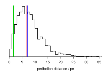
Figure 7: Distribution of the perihelion distance (from the orbital integration of the 2000 surrogates) for Tyc 6528-980-1. The green, red, and blue lines (left to right) show the nominal, LMA, and median estimates. This demonstrates that the nominal estimate – from integrating the orbit of just the nominal data – can be very unrepresentative of the distribution we get when we account for the uncertainties in the data.

Their other encounter (Tyc 8088-631-1) shows a similar problem. They quote a perihelion distance of $0.37\pm 1.18$ pc, whereas I find $d_{\rm ph}^{\rm med}=1.2$ pc with a 90% CI of 0.6–5.9 pc, and the LMA puts it at 0.95 pc.

Bobylev & Bajkova list in their Table 3 several other encounters which they consider less reliable. These all have radial velocity uncertainties larger than 10 km s^-1, so didn’t enter my analysis. Bobylev & Bajkova do not mention several close several encounters which I find, even though their RAVE selection is more inclusive. This may be because they choose a smaller limit on perihelion distance.

4 Accounting for survey incompleteness

A search for stellar encounters is defined here as complete if it discovers all stars which come within a particular perihelion time and perihelion distance. Incompleteness arises when objects in this time/distance window are not currently observable. This may occur in a magnitude-limited survey because a star’s large distance may render it invisible. The completeness is quantified here by the function $C(t_{\rm ph},d_{\rm ph})$, which specifies the fraction of objects at a specified perihelion time and distance which are currently observable.

I estimate $C$ by constructing a model for encounters and determining their observability within a survey. The encounter data are not used. I first define a model for the distribution and kinematics of stars. In its most general form this is a six-dimensional function over position and velocity (or seven-dimensional function if we also include time evolution of the distributions). I then integrate the orbits of these stars to derive the probability density function (PDF) over perihelion time and distance, $P_{\rm mod}(t_{\rm ph},d_{\rm ph})$. (Below I neglect gravity, so this integration will be replaced by the LMA.) The subscript “mod” indicates this has been derived from the model and, crucially, has nothing to do with the potential non-observability of stars. I then repeat this procedure, but taking into account the selection function of the survey. In general this would involve a spatial footprint, an extinction map, as well as bright and faint magnitude limits and anything else which leads to stars not being observed. This allows us to derive $P^{*}_{\rm exp}(t_{\rm ph},d_{\rm ph})$, where the “exp” subscript indicates this is the distribution we expect to observe in the survey (the asterisk indicates this is not a normalized PDF; more on this later). As shown in appendix B, the ratio $P^{*}_{\rm exp}(t_{\rm ph},d_{\rm ph})/P_{\rm mod}(t_{\rm ph},d_{\rm ph})$ is the completeness function.

In principle we could extend the completeness function to also be a function of the perihelion speed, $\mathrm{v}_{\rm ph}$ (and also the three other perihelion parameters which characterize directions). But I will assume we are 100% complete in this parameter, i.e. we don’t fail to observe stars on account of their kinematics.

4.1 The model

I implement the above approach using a very simple model for the encountering stars. Let $r$ be the distance from the Sun to a star of absolute magnitude $M$ and space velocity (relative to the Sun) $\mathrm{v}$. My assumptions are as follows:

1. the stellar spatial distribution is isotropic, described by $P(r)$.

2. the stellar velocity distribution is isotropic and homogeneous, described by $P(\mathrm{v})$;

3. the stellar luminosity function, $P(M)$, is homogeneous;

4. there is no extinction;

5. stellar paths are linear (no gravity);

6. the survey selection function, $S(m)$, is only a function of the apparent magnitude $m$. It specifies the fraction of objects observed at a given magnitude.

Note that $P(r)$, $P(\mathrm{v})$, and $P(M)$ are all one-dimensional functions, which will greatly simplify the computation of $P_{\rm mod}(t_{\rm ph},d_{\rm ph})$ and $P^{*}_{\rm exp}(t_{\rm ph},d_{\rm ph})$. The symmetry in these assumptions means any distribution will be symmetric in time. We therefore only need to consider future encounters.

Although my model is very simple (see the end of this subsection), it turns out to be reasonably robust to some changes in the assumed distributions, as we shall see. This is because we are only interested in how $P_{\rm mod}(t_{\rm ph},d_{\rm ph})$ changes under the introduction of the selection function. The poorly-defined selection functions of the TGAS data and the RV catalogues mean we would gain little from constructing a more complex model, yet we would pay a price in interpretability.

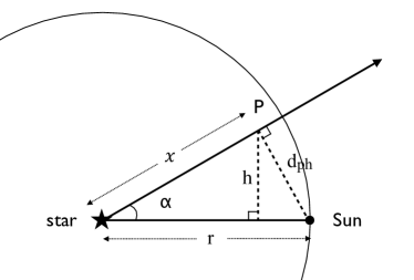
Figure 8: The geometry of a close encounter for a star initially at distance $r$ and reaching a perihelion distance of $d_{\rm ph}$ at point $P$, whereby $d_{\rm ph}\leq r$.

Using these assumptions I now derive $P(t_{\rm ph},d_{\rm ph})$. The initial steps are valid for both the “mod” and “exp” distributions, so I omit the subscripts where they are not relevant.

The geometry for an arbitrary star currently at distance $r$ from the Sun is shown in Figure 8. The star travels a distance $x$ to reach perihelion at point $P$, when its distance from the Sun is $d_{\rm ph}$. Note that $d_{\rm ph}\leq r$, otherwise the star has already been at perihelion (and I neglect past encounters due to time symmetry). To achieve a perihelion between distance $d_{\rm ph}$ and $d_{\rm ph}+\delta d_{\rm ph}$, this star must pass through a circular ring of inner radius $h$ and infinitesimal width $\delta d_{\rm ph}$. Note that $\delta d_{\rm ph}$ is parallel to $d_{\rm ph}$ and so perpendicular to the direction of motion. The area of this circular ring as seen from the initial position of the star is therefore $\delta A=2\pi h\delta d_{\rm ph}$, its circumference times its width. As all directions of travel for the star are equally probable (isotropic velocity distribution), the probability that this star has a perihelion distance between $d_{\rm ph}$ and $d_{\rm ph}+\delta d_{\rm ph}$ is just proportional to $\delta A$. That is

$$P(d_{\rm ph}\hskip 0.50003pt|\hskip 0.50003ptr)\,\delta d_{\rm ph}\, \propto\,\delta A\ ,\hskip 5.0pt{\rm so}$$ (2)

$$P(d_{\rm ph}\hskip 0.50003pt|\hskip 0.50003ptr)\, \propto\,h\ .$$ (3)

From the diagram we see that

$$\sin\alpha\,=\,\frac{d_{\rm ph}}{r}\,=\,\frac{h}{x}$$ (4)

and

$$x^{2}=r^{2}-d_{\rm ph}^{2}$$ (5)

from which it follows that

$$h\,=\,d_{\rm ph}\left(1-\frac{d_{\rm ph}^{2}}{r^{2}}\right)^{1/2}\ .$$ (6)

We can normalize analytically to get

$$P(d_{\rm ph}\hskip 0.50003pt|\hskip 0.50003ptr)\,=\,\frac{3d_{\rm ph}}{r^{2}}\left(1-\frac{d_{\rm ph}^{2}}{r^{2}}\right)^{1/2}\hskip 5.0pt{\rm where}\hskip 5.0ptd_{\rm ph}\leq r\ .$$ (7)

Plots of this distribution for different values of $r$ are shown in Figure 9. This may be counter-intuitive. For fixed $r$ the PDF is proportional to $h$ (equation 3). As we increase $d_{\rm ph}$ from zero, $h$ initially increases from zero. As the line Sun–P is always perpendicular to the line P–star, increasing $d_{\rm ph}$ beyond some point leads to $h$ decreasing. The PDF therefore has a maximum at $d_{\rm ph}<r$.

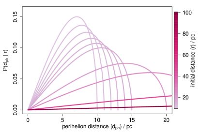
Figure 9: The PDF over the perihelion distance for stars with different initial distances $r=10,11,12,13,14,15,20,25,50,100$ pc, shown in different colours, as described by the model (section 4.1). The lines for $r>20$ pc extend beyond the right boundary of the plot, but have the same shape, dropping to zero at $d_{\rm ph}=r$.

We now compute the distribution over perihelion times. As velocities are constant, the time of the encounter, $t_{\rm ph}$, is $c_{0}x/\mathrm{v}$, where $\mathrm{v}$ is the velocity. Using parsecs for distance, years for time, and km s^-1 for velocity, $c_{0}=0.97779\times 10^{6}$. For a given $x$ there is a one-to-one correspondence between $\mathrm{v}$ and $t_{\rm ph}$. As $x$ is determined by $d_{\rm ph}$ and $r$, this means we can write

$$P(t_{\rm ph}\hskip 0.50003pt|\hskip 0.50003ptd_{\rm ph},r)\,\mathrm{d}t_{\rm ph}\,=\ P(\mathrm{v}\hskip 0.50003pt|\hskip 0.50003ptd_{\rm ph},r)\,\mathrm{d}\mathrm{v}.$$ (8)

Because we are assuming an isotropic and homogeneous velocity distribution, $P(\mathrm{v})$, we can write the term on the right as $P(\mathrm{v})\,\mathrm{d}\mathrm{v}$. It then follows that

$$P(t_{\rm ph}\hskip 0.50003pt|\hskip 0.50003ptd_{\rm ph},r)\, =\ P(\mathrm{v})\left|\frac{\mathrm{d}\mathrm{v}}{\mathrm{d}t_{\rm ph}}\right|$$ (9)

$$=\ P\left(\mathrm{v}=\frac{c_{0}x}{t_{\rm ph}}\right)\frac{c_{0}x}{t_{\rm ph}^{2}}\hskip 5.0pt{\rm where}\hskip 5.0ptd_{\rm ph}\leq r$$ (10)

with $x$ given by equation 5. This distribution is normalized (provided $P(\mathrm{v})$ is).

The model PDF we want is related to the two PDFs we just derived by marginalization, namely

$$P_{\rm mod}(t_{\rm ph},d_{\rm ph})\,=\ \int_{d_{\rm ph}}^{\infty}P(t_{\rm ph}\hskip 0.50003pt|\hskip 0.50003ptd_{\rm ph},r)P(d_{\rm ph}\hskip 0.50003pt|\hskip 0.50003ptr)P_{\rm mod}(r)\,\mathrm{d}r\ .$$ (11)

Typically, this integral must be computed numerically. I do this below by integrating on a grid.

The impact of the selection function is to reduce the number of stars we would otherwise see. The selection function depends only on apparent magnitude which, as I neglect extinction, is $m=M+5(\log r-1)$. Consequently the selection function only modifies the distance distribution, $P_{\rm mod}(r)$, to become

$$P^{*}_{\rm exp}(r)\,=\,P_{\rm mod}(r)\int_{-\infty}^{+\infty}P(M)S(m)\,\mathrm{d}M\ .$$ (12)

This PDF is not normalized (I use the asterisk to remind us of this). As $0\leq S(m)\leq 1$, $P^{*}_{\rm exp}(r)\leq P_{\rm mod}(r)$ for all $r$, i.e. the change from $P_{\rm mod}(r)$ to $P^{*}_{\rm exp}(r)$ reflects the absolute decrease in the distribution due to the selection function. This integral I also evaluate on a grid. The expected PDF over the perihelion time and distance is then

$$P^{*}_{\rm exp}(t_{\rm ph},d_{\rm ph})\,=\ \int_{d_{\rm ph}}^{\infty}P(t_{\rm ph}\hskip 0.50003pt|\hskip 0.50003ptd_{\rm ph},r)P(d_{\rm ph}\hskip 0.50003pt|\hskip 0.50003ptr)P^{*}_{\rm exp}(r)\,\mathrm{d}r$$ (13)

which is also not normalized. The completeness function is defined as

$$C(t_{\rm ph},d_{\rm ph})\,=\,\frac{F_{\rm exp}(t_{\rm ph},d_{\rm ph})}{F_{\rm mod}(t_{\rm ph},d_{\rm ph})}\ .$$ (14)

where $F_{\rm mod}(t_{\rm ph},d_{\rm ph})$ and $F_{\rm exp}(t_{\rm ph},d_{\rm ph})$ are the model and expected encounter flux – number of encounters per unit perihelion time and distance – respectively. As shown in appendix B, the completeness can be written as

$$C(t_{\rm ph},d_{\rm ph})\,=\,\frac{P^{*}_{\rm exp}(t_{\rm ph},d_{\rm ph})}{P_{\rm mod}(t_{\rm ph},d_{\rm ph})}\ ,$$ (15)

which is the ratio of the two PDFs I just derived. For all $t_{\rm ph}$ and $d_{\rm ph}$, $0\leq C(t_{\rm ph},d_{\rm ph})\leq 1$. This completeness function gives the probability (not probability density!) of observing an object at a given perihelion time and distance. I will use it in section 4.3 to infer the encounter rate.

Figure 10: The input distributions for the completeness model are the (a) distance (solid line), (b) space velocity, (c) absolute magnitude (normalized PDFs). The selection function (on apparent magnitude) is shown in panel (d). This modifies the model distance distribution to become the expected distribution shown as the dashed line in panel (a).

To compute the completeness function we need to select forms for the various input distributions. These are shown in Figure 10. For the distance distribution I use an exponentially decreasing space density distribution (Bailer-Jones, 2015b)

$$P_{\rm mod}(r)\,=\,\frac{1}{2L^{3}}\,r^{2}e^{-r/L}\hskip 5.0pt{\rm where}\hskip 5.0ptr>0$$ (16)

and $L$ is a length scale, here set to 100 pc. This produces a uniform density for $r\ll L$. This is shown in panel (a) as the solid line. This form has been chosen mostly for convenience, with a length scale which accommodates the decrease in density due to the disk scale height. The dashed line in panel (a) is $P^{*}_{\rm exp}(r)$. As expected, the selection function reduces the characteristic distance out to which stars can be seen. Panels (b) and (c) show the velocity and absolute magnitude distributions respectively. These are both implemented as shifted/scaled beta distributions, so are zero outside the ranges plotted. Again these have been chosen mostly for convenience. The luminosity distribution is a rough fit to the distribution in Just et al. (2015), with a smooth extension to fainter magnitudes. The lower end of the velocity distribution is a reasonable fit to the TGAS stars, but I have extended it to larger velocities to accommodate halo stars. This distribution ignores the anisotropy of stellar motions near to the Sun (e.g. Feng & Bailer-Jones, 2014). But as I am not concerned with the $(l,b)$ distribution of encounters, this is not too serious (I effectively average over $(l,b)$). None of these distributions is particularly realistic, but are reasonable given the already limiting assumptions imposed at the beginning of this section. Earlier attempts at completeness correction for encounter studies used even simpler assumptions. In section 4.5 I investigate the sensitivity of the resulting completeness function to these choices. Panel (d) models the TGAS selection function, as derived from the information given in Høg et al. (2000) and Lindegren et al. (2016). Due to the preliminary nature of the TGAS astrometric reduction, the complex selection function of the Tycho catalogue, and what was included in TGAS, this is a simple approximation of the true (unknown) TGAS selection function. In practice the selection function does not depend only on apparent magnitude. In particular, there are some bright stars fainter than my bright limit of G=4.5 that are not in TGAS. The only way to accommodate for such an incompleteness would be to inflate the encounter rate based on other studies, but this comes with its own complications, such as how to model their incompletenesses. The goal in the present work is to explore the consequences of a very simple model. Once we have data with better-defined selection functions, more complex – and harder to interpret – models will become appropriate and necessary.

4.2 Model predictions

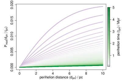
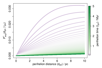
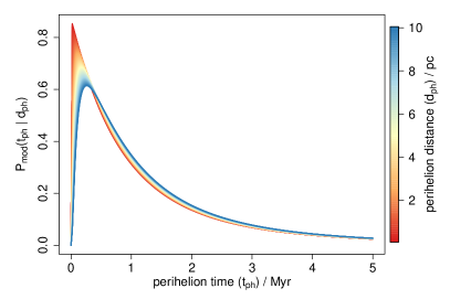
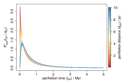
Figure 11: The distribution of stellar encounters in the model (left column of plots) and what we expect to observe from this model given the selection function (right column). The top row of plots shows the two-dimensional PDFs $P_{\rm mod}(t_{\rm ph},d_{\rm ph})$ (left) and $P^{*}_{\rm exp}(t_{\rm ph},d_{\rm ph})$ (right) on a colour scale in units Myr^-1pc^-1. The colour scale covers the full range of densities plotted (and is different in the two cases, being a factor of 4.4 larger for the model). The middle row shows the one-dimensional conditional PDFs over perihelion distance for different values of $t_{\rm ph}$ ranging from 100 kyr to 5 Myr in steps of 20 kyr. These are vertical cuts through the two-dimensional PDF (and re-normalized, as given by equation 17 for the model distribution). The bottom row shows the one-dimensional conditional PDFs over perihelion time for different values of $d_{\rm ph}$ ranging from 0.1 pc to 10 pc in steps of 0.1 pc. Only the positive perihelion times are shown for the four conditional plots, which also use different density scales (vertical axes).

Using these input distributions, the resulting distribution $P_{\rm mod}(t_{\rm ph},d_{\rm ph})$ for the model is shown in the top left panel of Figure 11. The distribution we expect to observe – i.e. after application of the selection function – is show in the top right panel. The one-dimensional conditional distributions derived from these, e.g.

$$P_{\rm mod}(d_{\rm ph}\hskip 0.50003pt|\hskip 0.50003ptt_{\rm ph})\,=\,\frac{P_{\rm mod}(t_{\rm ph},d_{\rm ph})}{\int_{0}^{\infty}P_{\rm mod}(t_{\rm ph},d_{\rm ph}^{\prime})\,\mathrm{d}d_{\rm ph}^{\prime}}$$ (17)

are shown in the bottom two rows.

By construction, these distributions are symmetric about $t_{\rm ph}=0$. Consider the form of $P_{\rm mod}(t_{\rm ph}\hskip 0.50003pt|\hskip 0.50003ptd_{\rm ph})$ in the bottom left panel of Figure 11. This increases from zero at $t_{\rm ph}=0$ to a maximum somewhere between 0 and 0.25 Myr (depending on $d_{\rm ph}$) before decreasing at larger $t_{\rm ph}$. This can be understood from the encounter geometry and the combination of the input distance and velocity distributions. Stars that encounter in the very near future are currently nearby (small $r$), but “nearby” has a limited volume ($\propto r^{3}$) and so a limited supply of stars. Thus the further into the future encounters occur, the more volume there is available for their present positions, so – provided the space density doesn’t drop – the more encounters there can be. This explains the increase in $P_{\rm mod}(t_{\rm ph}\hskip 0.50003pt|\hskip 0.50003ptd_{\rm ph})$ at small $t_{\rm ph}$. But at large enough distances the space density of stars does drop (Figure 10a), so the number of potentially encountering stars also decreases. These currently more distant stars generally have encounters further in the future, which is why $P_{\rm mod}(t_{\rm ph}\hskip 0.50003pt|\hskip 0.50003ptd_{\rm ph})$ decreases at larger $t_{\rm ph}$. Stars coming from $L=100$ pc (where the space density has dropped off by a factor of $e^{-1}$) with the most common space velocity (60 km s^-1, the mode of $P(\mathrm{v})$ in Figure 10b) take 1.7 Myr to reach us, and we see in the figure that $P_{\rm mod}(t_{\rm ph}\hskip 0.50003pt|\hskip 0.50003ptd_{\rm ph})$ has already dropped significantly by such times.

The $P(t_{\rm ph},d_{\rm ph})$ distribution is not invariant under translations in the perihelion time, but this does not mean we are observing at a privileged time. After all, there is no time evolution of the stellar population in our model, so we would make this same prediction for any time in the past or future. It is important to realise that Figure 11 shows when and where stars which we observe now will be at perihelion. The drop-off at large perihelion times is a result of the adopted spatial and velocity distributions. In some sense these distributions are not self-consistent, because this velocity distribution would lead to a changing spatial distribution.

Other than for very small values of $t_{\rm ph}$, we see that $P_{\rm mod}(d_{\rm ph}\hskip 0.50003pt|\hskip 0.50003ptt_{\rm ph})$ increases linearly with $d_{\rm ph}$ over the perihelion distances shown (0–10 pc). The number of encounters occurring within a given distance, which is proportional to the integral of this quantity, therefore varies as $d_{\rm ph}^{2}$. This behaviour may seem counter-intuitive (e.g. for a uniform density, the number of stars within a given distance grows as the cube of the distance). But it can again be understood when we consider the phase space volume available for encounters: In order for a star to encounter at a distance $d_{\rm ph}$ of the Sun, it must traverse a thin spherical shell (centered on the Sun) of radius $d_{\rm ph}$. The volume of this shell scales as $d_{\rm ph}^{2}$, so the number of stars traversing this volume also scales as $d_{\rm ph}^{2}$. Thus the number of encounters per unit perihelion distance, which is proportional to $P_{\rm mod}(d_{\rm ph}\hskip 0.50003pt|\hskip 0.50003ptt_{\rm ph})$, scales as $d_{\rm ph}$, as the model predicts. This will break down at large $d_{\rm ph}$, because even though the phase space available for encountering continues to grow, the number of stars available to fill it does not, because of the form of $P_{\rm mod}(r)$. Thus $P_{\rm mod}(d_{\rm ph}\hskip 0.50003pt|\hskip 0.50003ptt_{\rm ph})$ will decrease for sufficiently large $d_{\rm ph}$ (which anyway must occur, because the PDF is normalized). Examination of $P_{\rm mod}(d_{\rm ph}\hskip 0.50003pt|\hskip 0.50003ptt_{\rm ph})$ out to much larger distances than those plotted confirms this. There is a second contribution to this turn-over, namely that at smaller $t_{\rm ph}$ the volume from which the encounters can come is also smaller (as explained earlier). Thus for these times we begin to “run out” of encounters already at smaller values of $d_{\rm ph}$. This can be seen as a levelling-off of $P_{\rm mod}(d_{\rm ph}\hskip 0.50003pt|\hskip 0.50003ptt_{\rm ph})$ at very small $t_{\rm ph}$ in Figure 11 (upper lines in middle left panel).

The expected distributions (the right column of Figure 11) are qualitatively similar to the model distributions. The main difference is that the expected distribution is squeezed toward closer times. This is consistent with the fact that we only observe the brighter and therefore generally nearer stars in our survey, which correspondingly have smaller encounter times.

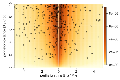
Figure 12: As the top right panel of Figure 11, now overplotted with the TGAS encounters found using the linear motion approximation $(t_{\rm ph}^{\rm lin},d_{\rm ph}^{\rm lin})$, with duplicates removed at random.

Figure 12 overplots the perihelion times and distances of the TGAS encounters with this expected distribution. For this plot I have used the encounters as found with the linear motion approximation, rather than with the orbit integrations, because the latter will be incomplete near to 10 pc (as explained in section 2). I show only the 439 unique stars (rather than all objects), with duplicates removed at random. As the model is very simple we do not expect good agreement with the observations. But the data show a similar distribution, in particular fewer encounters both at large times and at times near to zero. Recall that the encounter model shows an intrinsic minimum – in fact a zero – at $t_{\rm ph}=0$, i.e. it is not due to observational selection effects. Rather it is due to the vanishing amount of phase space available for encountering stars as $t_{\rm ph}$ decreases to zero. So we expect to see this in the data. While we see it here, it is not clearly discernable in my earlier Hipparcos-based study (Figure 2 of paper 1).

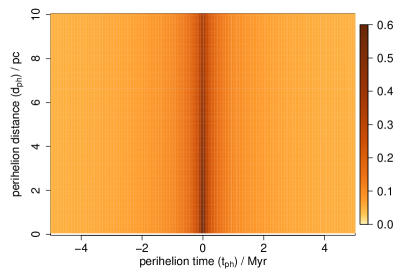
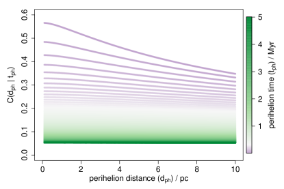
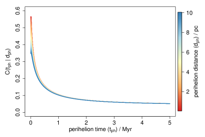
Figure 13: The completeness function, $C(t_{\rm ph},d_{\rm ph})$ (top panel). This shows the probability of observing an encounter as a function of its perihelion time and distance. It uses distributions of stellar properties and an approximation of the TGAS selection function (see section 4.1) and is mirror-symmetric about $t_{\rm ph}=0$. The values shown range between 0.05 and 0.57, which excludes $t_{\rm ph}=0$ and $d_{\rm ph}=0$ as formally the incompleteness is undefined at these values. Cuts through this parallel to the $d_{\rm ph}$ axis are shown in the middle panel for $t_{\rm ph}$ from 20 kyr to 5 Myr in steps of 20 kyr. Cuts parallel to the $t_{\rm ph}$ axis (for positive $t_{\rm ph}$) are shown in the bottom panel for $d_{\rm ph}$ from 0.1–10 pc in steps of 0.1 pc.

The completeness function (computed with equation 15) is shown in the top panel of Figure 13. Formally $C(t_{\rm ph}=0,d_{\rm ph})$ and $C(t_{\rm ph},d_{\rm ph}=0)$ are undefined (zero divided by zero), but given the time symmetry and the form of the plots, it is clear that at fixed $d_{\rm ph}$ the function varies continuously at $t_{\rm ph}=0$, so I use constant interpolation to fill this. The true completeness will not go to unity at $t_{\rm ph}=0$ for very small $d_{\rm ph}$, because such encountering stars would currently be so close and hence some so bright that they would be unobservable due to the bright limit of the selection function. I avoid the formal singularity at $d_{\rm ph}=0$ in the following by using a lower limit of $d_{\rm ph}=0.1$ pc. This and the constant interpolation have negligible impact on the following results.

We see from Figure 13 that the completeness ranges from 0.05 at large perihelion times to 0.57 for very close times. The mean completeness for $|t_{\rm ph}|<5$ Myr and $d_{\rm ph}<5$ pc is 0.091 (0.099 for $d_{\rm ph}<2$ pc). That is, if all TGAS stars had measured radial velocities, we would expect to observe about 1 in 11 of the encountering stars in this region (if the Galaxy really followed the model assumptions laid out above). This might seem a rather large fraction, given that Figure 10(a) shows a much smaller fraction of stars retained when the selection function is applied to $P_{\rm mod}(r)$ (solid line) to achieve $P^{*}_{\rm exp}(r)$. But $P^{*}_{\rm exp}(r)$ shows the observability of all stars, not just the encountering stars. A completeness correction based on the observability of all stars would be incorrect, because it would “overcorrect” for all those stars which won’t be close encounters anyway.

There is very little dependence of the completeness on distance, except at the smallest times, as can be seen in the middle panel of Figure 13, which shows cuts through the completeness at fixed times. At $t_{\rm ph}=1$ Myr, for example, the completeness varies from 0.106 at $d_{\rm ph}=0.1$ pc to 0.102 at $d_{\rm ph}=10$ pc. There is a strong dependence on time, in contrast, as can be seen in the bottom panel of Figure 13. The lack of distance dependence is because, for a given encounter time, those stars which encounter at 0.1 pc have much the same current spatial distribution as those which encounter at 10 pc: They all come from a large range of distance which is much larger than 10 pc (unless $t_{\rm ph}$ is very small), so their average observability and thus completness is much the same. Perihelion times varying between 0 and 5 Myr, in contrast, correspond to populations of stars currently at very different distances, for which the observability varies considerably.

4.3 An estimate of the encounter rate

I now use the completeness function to correct the observed distribution of encounters in order to infer the intrinsic (“true”) distribution of encounters. From this we can compute the current encounter rate out to some perihelion distance.

Let $F_{\rm int}(t_{\rm ph},d_{\rm ph})$ be the intrinsic distribution of encounters, i.e. the number of encounters per unit perihelion time and perihelion distance with perihelion parameters $(t_{\rm ph},d_{\rm ph})$. The corresponding quantity for the observed encounters is $F_{\rm obs}(t_{\rm ph},d_{\rm ph})$. These two quantities are the empirical equivalents of $F_{\rm mod}$ and $F_{\rm exp}$, respectively, introduced around equation 14. This equation therefore tells us that

$$F_{\rm obs}(t_{\rm ph},d_{\rm ph})\,=\,gC(t_{\rm ph},d_{\rm ph})F_{\rm int}(t_{\rm ph},d_{\rm ph})$$ (18)

where $g$ is an extra factor accommodating the possibility that the search for encounters did not include all the observed stars (discussed below). Given this factor, the completeness function, and the observed distribution of encounters, we can derive $F_{\rm int}(t_{\rm ph},d_{\rm ph})$. Integrating this over time and distance we infer the intrinsic number of encounters.

To do this I first represent the observed encounter distribution, $F_{\rm obs}(t_{\rm ph},d_{\rm ph})$, as a continuous density. I compute this using kernel density estimation (with a Gaussian kernel) on the surrogates for all stars. (The surrogates are the data resamples in the orbital integration – see item 5 in section 2). By applying the density estimation to the surrogates – rather than, say, the median of the perihelion parameter distribution – we account for the uncertainties. When computing the density I only retain unique stars (duplicates are removed at random). I also exclude surrogates with $\mathrm{v}_{\rm ph}>300$ km s^-1, on the grounds that the model does not include faster stars either. This also gets rid of objects with the most spurious radial velocity measurements.

Figure 14 shows the resulting distribution. The density scale has been defined such that the integral over some perihelion time and distance region equals the (fractional) number of stars within that region. This number can be a fraction because not all of the surrogates for a star lie within the region.

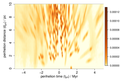
Figure 14: The density of the observed encounters, $F_{\rm obs}(t_{\rm ph},d_{\rm ph})$, estimated by kernel density estimation over the surrogates (orbital-integrated data samples) with $\mathrm{v}_{\rm ph}\leq 300$ km s^-1, for all unique stars. The colour scale gives the number of encounters per unit time and distance. The integral over time and distance is the (fractional) number of encountering stars.

The completeness function describes what fraction of stars we miss on account of the TGAS selection function. But it does not reflect the fact that not all TGAS stars have radial velocities, and so could not even be tested for being potential encounters. This is accommodated by the factor $g$ in equation 18. The total number of stars in TGAS is 2 057 050 (Lindegren et al., 2016, section 5.1). The number of stars in TGAS for which I have valid radial velocities is 322 462, and this is approximately the number of stars which I could potentially have searched for encounters. Therefore, the fraction of stars in TGAS I effectively searched is $g=322\,462/2\,057\,050=0.157$.

I now apply equation 18 to find $F_{\rm int}(t_{\rm ph},d_{\rm ph})$. Integrating this over some region of $t_{\rm ph}$ and $d_{\rm ph}$ gives the inferred number of encounters in that region. Dividing that by the time range of the region gives the average encounter rate.

For the full region over which the completeness has been computed, $|t_{\rm ph}|\leq 5$ Myr and $d_{\rm ph}\leq 10$ pc, the inferred encounter rate is $2117\pm 115$ Myr^-1. The quoted uncertainty reflects only the Poisson uncertainty arising from the finite number of observed encounters (it is the rate divided by the square root of the fractional number of encounters). This rate is likely to be an underestimate, however, because we will miss encounters near to 10 pc on account of the initial LMA-based selection (explained at the end of section 2). Limiting the region to perihelion distances within 5 pc we get $545\pm 59$ Myr^-1. This is 3.9 times smaller, which follows almost exactly the quadratic dependence on the number of encounters within a given distance predicted by the encounter model (see section 4.2).

If I limit the region to 2 pc we get an encounter rate of $124\pm 30$ Myr^-1. However, this estimate is based primarily on just the 13 stars with $d_{\rm ph}^{\rm med}<2$ pc and $\mathrm{v}_{\rm ph}^{\rm med}<300$ km s^-1, so has a larger uncertainty. If I instead scale quadratically the result for 5 pc, I get $87\pm 9$ Myr^-1, which is what I adopt as the rate inferred by this study.

The inferred encounter rates for smaller time windows tend to be higher. For $d_{\rm ph}\leq 5$ pc, the average rates for close encounters within 1, 2, 3, and 4 Myr of now are $844\pm 128$, $816\pm 102$, $725\pm 83$, and $639\pm 70$ Myr^-1 respectively. These are consistent within the quoted uncertainties, although these estimates are not independent because encounters in the shorter time intervals are also counted in the longer intervals.

4.4 Other published rates

Other authors have derived encounter rates using different data sets or from Galaxy models. Using the Hipparcos catalogue and a correction for incompleteness, García-Sánchez et al. (2001) derived a value of $11.7\pm 1.3$ Myr^-1 within 1 pc (an average for the past and future 10 Myr, it seems). Applying the quadratic scaling with distance, this would correspond to $46.8\pm 5.2$ Myr^-1 within 2 pc, which is about half the size of my result. Their approach to the incompleteness is very different: they compute a single factor for the fraction of stars within 50 pc which Hipparcos did not see (estimated as $1/5$), even though many of their encounters would have travelled from much larger distances. My correction, in contrast, looks at the completeness as a function of encounter time and distance, based on non-uniform density and velocity distributions. The luminosity function they used in their correction (their Figure 13) does not include nearly as many faint stars as mine (Figure 10c). This may explain their smaller inferred encounter rate.

Martínez-Barbosa et al. (2017) used N-body simulations of the Galaxy for three different scenarios – with orbital migration from the inner disk, no significant migration, and with migration from the outer disk – to derive current encounter rates of 21, 39, and 63 Myr^-1 within 1.94 pc, respectively. These are all somewhat smaller than my inferred rate for the same distance.

4.5 Sensitivity to assumptions

My completeness model contains a number of simplifying assumptions, so I look here briefly at their impact on the completeness function and the derived encounter rate.

The adopted distance distribution (equation 16, Figure 10a) uses a length scale of $L=100$ pc. If I double this, then the model distribution $P_{\rm mod}(t_{\rm ph}\hskip 0.50003pt|\hskip 0.50003ptd_{\rm ph})$ shown in the bottom left panel of Figure 11 is stretched in time, because the bulk of the stars are now further away and so take longer to reach perihelion. The expected distribution (bottom right panel of Figure 11) stretches in a similar way. The net result is a decrease in completeness, as we would expect, because the stars are now more distant and so less observable. The mean completeness for $|t_{\rm ph}|<5$ Myr and $d_{\rm ph}<5$ pc is 0.078 (compared to 0.091 before). Using this completeness function, the inferred encounter rate over the past/future 5 Myr within 5 pc is $659\pm 71$ Myr^-1, compared to 545 Myr^-1 computed earlier with $L=100$ pc.

In the orignal model I assumed that the velocity distribution of stars was as shown in Figure 11(b). I now scale this distribution in velocity by a factor of two, keeping the shape the same (i.e. the mode shifts from 60 km s^-1 to 120 km s^-1). As the stars are now moving much faster, we see relatively more encounters at closer times in the past/future (and likewise fewer at large times), because their travel times to encounter are shorter. The conditional distributions are compressed considerably compared to the nominal case. The mean completeness for $|t_{\rm ph}|<5$ Myr and $d_{\rm ph}<5$ pc is now decreased to 0.069, and the inferred encounter rate over this region is $782\pm 81$ Myr^-1, 1.4 times larger than before. (Scaling the velocities by a factor of a half – so the mode is 30 km s^-1 rather than 60 km s^-1 – lowers the encounter rate by the same factor.)

In reality, TGAS does not have the sharp bright-magnitude cut I use in the model (Figure 10d). I set this to $G=4.5$ on the grounds that there is only one star brighter in TGAS. Modelling the shape of the completeness at the bright end using very few stars is difficult, so I test the sensitivity to this choice by shifting the cut-off to $G=5.5$ (375 TGAS stars are brighter than this). Remodelling the completeness, I find that the inferred encounter rate increases by just 1%. This is an increase and not a decrease because while the number of observed encounters stays the same, $P^{*}_{\rm exp}$ and therefore $C$ are slightly smaller, thus increasing $F_{\rm int}$ (see equations 15 and 18).

These tests indicate that while the incompleteness-corrected encounter rate does depend on the assumed model parameters, it is not overly sensitive. Of course, the model remains rather unrealistic, not least the assumption of isotropic and independent distance and velocity distributions. Changes to these could have a more dramatic impact. On the other hand, the completeness function depends not on the model directly, but only on how the derived encounter distribution changes under the observational selection function, which is a weaker dependence. Nonetheless, for the deeper survey we expect in the second Gaia data release, a more sophisticated model should be adopted.

5 Summary and conclusions

I have searched for close stellar encounters using a combination of Gaia astrometry and several radial velocity catalogues. Candidates were identified from a list of 322 462 stars by assuming that stars travel on straight lines relative to the Sun, and identifying those which come within 10 pc. The orbits of these were then integrated in a Galactic potential to compute more precise perihelion parameters. This included an integration of resampled data (“surrogates”) in order to determine the (asymmetric) distribution over the perihelion time, distance, and speed for each star. These distributions are summarized with the 5%, 50% (median), and 95% percentiles (Table 3).

16 stars were found to have median perihelion distances less than 2 pc (see Table 2). This is fewer than I found in my Hipparcos-based study (paper 1), and fewer than expected given the much larger size of TGAS (it has 17 times more stars than Hipparcos, although due to the limited availability of radial velocities it is effectively only four times larger). This is in part because TGAS includes fewer bright stars (only one brighter than $G=4.5$ mag), but also because I have excluded stars with large radial velocity uncertainties. Note that some of the encounters listed are almost certainly spurious due, for example, to implausibly large radial velocity measurements.

The closest encounter found is Gl 710, known for some time to come close to the Sun. TGAS determines a smaller proper motion than Hipparcos for this star, leading to a much smaller perihelion distance: now just 16 000 AU (90% CI 10 000–21 000 AU), making Gl 710 the closest approaching star known. This brings it within the Oort cloud, and although its mass is low, so is its velocity, so its perturbing influence is likely to be much higher than more massive but more distant encounters (Figure 6).

I then set up simple models for the stellar spatial, velocity, and luminosity distributions and used these to compute the perihelion distribution we would observe in the absence of observational selection effects (left column of Figure 11). This shows, for example, a decrease in the number of encounters at larger absolute perihelion times. This is a direct (and possibly counter-intuitive) consequence of the adopted spatial and velocity distributions. I then determined how this distribution would change under the influence of the TGAS selection function (right column of Figure 11). The ratio of this expected distribution to the model distribution gives the completeness function (Figure 13). This tells us that the probability that TGAS observes a star which encounters within 2 pc within 5 Myr of now is on average 0.09 (and 0.20 within 1 Myr from now). This function shows very little change in the completeness out to 10 pc perihelion distance, but a strong drop off with perihelion time over $\pm 5$ Myr. This is also seen in the distribution of observed encounters. I emphasize that the completeness model is based on very simple assumptions, in particular isotropic spatial and homogeneous velocity distributions, and a selection function which only depends on magnitude. A more complex model would bring few benefits for these data, because the selection functions for TGAS and the RV catalogues would still be poorly defined. The goal in this paper was to explore the consequences of a simple model; this will help the interpretation of more complex models (to be developed for later Gaia data releases). Yet even my simple model is an improvement on earlier attempts at deriving encounter rates, which have either ignored incompleteness or have assumed uniform distributions. Moreover, this is the first study to look at the completeness in the parameter space of interest, which is where we actually need it.

Combining the completeness function with the number of observed encounters (excluding those with $|\mathrm{v}_{r}|>300$ km s^-1), and taking into account that not all TGAS stars had radial velocities, I estimated the intrinsic encounter rate. Averaged over the past/future 5 Myr this is $545\pm 59$ Myr^-1 for encounters within 5 pc. My model predicts that this scales quadratically with the distance limit. This is confirmed by the data, as the incompleteness-corrected rate out to twice this distance is $2117\pm 115$ Myr^-1, a factor $3.9\pm 0.4$ larger. Thus the implied encounter rate within 1 pc (scaling from the 5 pc result) is $21.8\pm 2.4$ Myr^-1. The quoted uncertainties reflect only Poisson uncertainties in the detected encounters; uncertainties due to model approximations are probably larger. The rates given are for all types of stars, as defined by the luminosity distribution in my model (Figure 10c). As the true luminosity distribution is poorly sampled by TGAS, this is one source of additional uncertainty in my derived rates. In particular, TGAS omits more bright stars than my simple selection function accommodates, which would lead to my rates being slightly underestimated.

Some stars which are not both in TGAS and my radial velocity catalogues are additionally known to be close encounters (see references in the introduction). I have not included these in my analysis because cobbling together encounters found in different ways from different surveys makes modelling the incompleteness nearly impossible. The goal of the present paper was not to list all known close encounters, but rather to make a step toward a more complete modelling with later Gaia data releases.

6 Moving on: future Gaia data releases

The next Gaia data release (GDR2, planned for April 2018) should provide more precise parallaxes and proper motions for of order a billion stars down to $G\simeq 21$ and up to $G\simeq 4$. This will be vital for increasing the completeness of encounter searches, in particular to encounter times further in the past/future than a few Myr. Using my model together with an estimate of the GDR2 magnitude selection function, I compute the mean completeness over the range $d_{\rm ph}<2$ pc and $|t_{\rm ph}|<5$ Myr to be 0.75, eight times higher than TGAS. The completeness model in the present paper is too simplistic for GDR2, however, because GDR2 will include many more-distant stars. It should also have a better-defined selection function (among other things, it will become independent of Tycho.) It will then be appropriate to construct a three-dimensional spatial model, as well as a three-dimensional velocity model with spatial dependence, in order to better model the Galaxy (different components, disk rotation, etc.).

The number of encounters which can be found in GDR2 will be limited by the availability of radial velocities. Although GDR2 will include estimates of radial velocities for a few million of the brightest stars (to a precision of a few km/s) – from the calcium triplet spectra observed by the satellite’s high resolution spectrograph (Gaia Collaboration et al., 2016b) – this remains a small fraction of stars with astrometry. Even upcoming large-scale spectroscopic surveys will obtain “only” tens of millions of spectra. We are now entering a period in which the ability to find encounters is limited not by the availability of astrometry, but by the availability of radial velocities. Furthermore, the Gaia astrometric accuracy is so good that the corresponding transverse velocity accuracy for encounter candidates will far exceed the precision of large-scale radial velocity surveys. Using the official predictions of the end-of-5-year-mission Gaia accuracy, a G-type dwarf at a distance of 200 pc moving with a transverse velocity of 5 km s^-1 will have this velocity determined to an accuracy of 8 m s^-1.

The following (third) Gaia data release will also include estimates of stellar masses and radii, derived by the DPAC using the low resolution Gaia spectroscopy, magnitude, parallax, and stellar models (Bailer-Jones et al., 2013). We will then be able to estimate systematically actual impulses (equation 1), and also to correct the measured radial velocities for the gravitational redshift, which is of order 0.5–1.0 km s^-1 (Pasquini et al., 2011). This data release should also include solutions for astrometric and spectroscopic binaries (Pourbaix, 2011), thereby permitting a better computation of flight paths for such systems.

Appendix A Gaia archive query

Below is the ADQL query used to select stars from the TGAS table which have perihelion distances less than 10 pc according to the linear motion approximation, assuming they all have $|\mathrm{v}_{r}|=750$ km s^-1. The TGAS table does not list Tycho IDs when Hipparcos IDs are present, so I use a join to add these missing Tycho IDs.

select tgas.tycho2_id, tycho2.id, tgas.hip,
tgas.source_id, tgas.phot_g_mean_mag, tgas.ra,
tgas.dec, tgas.parallax, tgas.pmra, tgas.pmdec,
tgas.ra_error, tgas.dec_error, tgas.parallax_error,
tgas.pmra_error, tgas.pmdec_error, tgas.ra_dec_corr,
tgas.ra_parallax_corr, tgas.ra_pmra_corr,
tgas.ra_pmdec_corr, tgas.dec_parallax_corr,
tgas.dec_pmra_corr, tgas.dec_pmdec_corr,
tgas.parallax_pmra_corr, tgas.parallax_pmdec_corr,
tgas.pmra_pmdec_corr
from gaiadr1.tgas_source as tgas
left outer join public.tycho2 as tycho2
on tgas.hip = tycho2.hip
where( ( 1000*4.74047*sqrt(power(tgas.pmra,2) +
  power(tgas.pmdec,2))/power(tgas.parallax,2) ) /
  ( sqrt( (power(tgas.pmra,2) + power(tgas.pmdec,2)) *
  power(4.74047/tgas.parallax,2) + power(750,2) ) )
  ) < 10

Appendix B The completeness function

Let $F_{\rm mod}(t_{\rm ph},d_{\rm ph})$ be the model-predicted number of encounters per unit perihelion time and perihelion distance at $(t_{\rm ph},d_{\rm ph})$, and let $F_{\rm exp}(t_{\rm ph},d_{\rm ph})$ be the corresponding expected quantity, i.e. after modulation by the observational selection function. The completeness function, $C(t_{\rm ph},d_{\rm ph})$, specifies the fraction of objects observed at a given $(t_{\rm ph},d_{\rm ph})$, and is defined by

$$F_{\rm exp}(t_{\rm ph},d_{\rm ph})\,=\,C(t_{\rm ph},d_{\rm ph})F_{\rm mod}(t_{\rm ph},d_{\rm ph})\ .$$ (19)

Clearly $0\leq C(t_{\rm ph},d_{\rm ph})\leq 1$. $P_{\rm mod}(t_{\rm ph},d_{\rm ph})$ is the normalized PDF of $F_{\rm mod}(t_{\rm ph},d_{\rm ph})$, i.e.

$$P_{\rm mod}(t_{\rm ph},d_{\rm ph})\,=\,\frac{F_{\rm mod}(t_{\rm ph},d_{\rm ph})}{\iint F_{\rm mod}(t_{\rm ph}^{\prime},d_{\rm ph}^{\prime})\,\mathrm{d}t_{\rm ph}^{\prime}\mathrm{d}d_{\rm ph}^{\prime}}\,=\,\frac{F_{\rm mod}(t_{\rm ph},d_{\rm ph})}{N_{\rm mod}}$$ (20)

where the integral is over all perihelion times and distances, which (conceptually) gives the total number of encounters in the model, $N_{\rm mod}$. (This is only a conceptual definition for $N_{\rm mod}$, because my model is continuous.) $P^{*}_{\rm exp}(t_{\rm ph},d_{\rm ph})$ relates to $F_{\rm exp}(t_{\rm ph},d_{\rm ph})$ in a similar way, but here we must include an additional (dimensionless) factor, $b$, to accommodate the fact that $P^{*}_{\rm exp}(t_{\rm ph},d_{\rm ph})$ is not normalized,

$$P^{*}_{\rm exp}(t_{\rm ph},d_{\rm ph})\,=\,\frac{b\,F_{\rm exp}(t_{\rm ph},d_{\rm ph})}{\iint F_{\rm exp}(t_{\rm ph}^{\prime},d_{\rm ph}^{\prime})\,\mathrm{d}t_{\rm ph}^{\prime}\mathrm{d}d_{\rm ph}^{\prime}}\,=\,\frac{b\,F_{\rm exp}(t_{\rm ph},d_{\rm ph})}{N_{\rm exp}}$$ (21)

which also defines $N_{\rm exp}$. Integrating both sides of this equation over all perihelion times and distances shows us that

$$b\,=\,\iint P^{*}_{\rm exp}(t_{\rm ph}^{\prime},d_{\rm ph}^{\prime})\,\mathrm{d}t_{\rm ph}^{\prime}\mathrm{d}d_{\rm ph}^{\prime}\ .$$ (22)

By construction $P^{*}_{\rm exp}(t_{\rm ph},d_{\rm ph})$ is the reduction in $P_{\rm mod}(t_{\rm ph},d_{\rm ph})$ under the influence of the selection function, so $P^{*}_{\rm exp}(t_{\rm ph},d_{\rm ph})\leq P_{\rm mod}(t_{\rm ph},d_{\rm ph})$ everywhere. Hence $b$, which therefore lies between 0 and 1, is the fraction of stars retained following application of the selection function, which is $N_{\rm exp}/N_{\rm mod}$.

Substituting $F_{\rm mod}(t_{\rm ph},d_{\rm ph})$ from equation 20 and $F_{\rm exp}(t_{\rm ph},d_{\rm ph})$ from 21 into equation 19 gives

$$C(t_{\rm ph},d_{\rm ph})\,=\,\frac{P^{*}_{\rm exp}(t_{\rm ph},d_{\rm ph})}{P_{\rm mod}(t_{\rm ph},d_{\rm ph})}\frac{N_{\rm exp}}{N_{\rm mod}}\frac{1}{b}\ .$$ (23)

But $b=N_{\rm exp}/N_{\rm mod}$, so

$$C(t_{\rm ph},d_{\rm ph})\,=\,\frac{P^{*}_{\rm exp}(t_{\rm ph},d_{\rm ph})}{P_{\rm mod}(t_{\rm ph},d_{\rm ph})}\ .$$ (24)