Efficient time stepping for the multiplicative Maxwell fluid including the Mooney-Rivlin hyperelasticity

Abstract

A popular version of the finite strain Maxwell fluid is considered, which is based on the multiplicative decomposition of the deformation gradient tensor. The model combines Newtonian viscosity with hyperelasticity of Mooney-Rivlin type; it is a special case of the viscoplasticty model proposed by Simo and Miehe (1992). A simple, efficient and robust implicit time stepping procedure is suggested. Lagrangian and Eulerian versions of the algorithm are available, with equivalent properties. The numerical scheme is iteration free, unconditionally stable and first order accurate. It exactly preserves the inelastic incompressibility, symmetry, positive definiteness of the internal variables, and w-invariance. The accuracy of the stress computations is tested using a series of numerical simulations involving a non-proportional loading and large strain increments. In terms of accuracy, the proposed algorithm is equivalent to the modified Euler backward method with exact inelastic incompressibility; the proposed method is also equivalent to the classical integration method based on exponential mapping. Since the new method is iteration free, it is more robust and computationally efficient. The algorithm is implemented into MSC.MARC and a series of initial boundary value problems is solved in order to demonstrate the usability of the numerical procedures.

Key words: finite strain, Maxwell fluid, multiplicative viscoelasticity, Mooney-Rivlin, implicit time stepping, efficient numerics

1 Introduction

The Maxwell fluid, also known as the Maxwell material (cf. [39]), is in the focus of the current research. Thanks to a special combination of elastic and viscous (inelastic) properties, it is widespread in the phenomenological material modelling. Apart from obvious applications to the dynamics of viscous fluids [1], different versions of the finite strain Maxwell model are employed for solid materials as well. A parallel connection of the Maxwell fluid with idealized elastic elements allows one to model the behaviour of polymers [31, 37, 17, 25, 5, 12, 24], biological tissues [22, 11, 26, 57], explosives [3] and other types of viscoelastic materials. Plasticity models with a nonlinear kinematic hardening may operate with backstresses; the evolution of the backstresses can be described using the Maxwell element as well [28, 4, 58, 10, 47]. A generalization of this approach to plasticity with the yield surface distortion is reported in [48, 49]. Some advanced models of shape memory alloys [18, 20] and anisotropic creep [53] include the Maxwell fluid as an important constituent. Interestingly, minor modifications of the Maxwell fluid are also used in production of mechanics-based computer animations [35]. Applications of the Maxwell fluid to the analysis of geological structures are reported in [42, 34]. Due to the high prevalence of the Maxwell concept in the phenomenological material modeling, specialized numerical algorithms with an enhanced robustness and efficiency are becoming increasingly important. High computational efficiency of the utilized algorithms may become especially important for real-time simulations, like FEM simulations of surgical operations [32].

Different mathematical formulations of the finite strain Maxwell fluid are currently in use (cf. [45]). We advocate here the multiplicative approach of Simo and Miehe [56], due to its numerous advantages like thermodynamic consistency, exact hyperelasticity, absence of spurious shear oscillations, pure isochoric-volumetric split [45], w-invariance under the isochoric change of the reference configuration [44] and exponential stability of the solution with respect to the perturbation of the initial data [46]. Within the approach of Simo and Miehe, the Newtonian viscosity can be combined with different types of isotropic elastic potentials in a thermodynamically consistent manner.

In computational practice, the implemented time step size can be larger than the relaxation time of a Maxwell element. For that reason, implicit integration of the six-dimensional evolution equation is needed. After the discretization in time, a system of six nonlinear equations with respect to six unknowns is obtained. Using the spectral decomposition, the number of unknowns can be reduced to three [55, 38, 21, 13]. Typically, these nonlinear systems of equations are solved iteratively using the Newton-Raphson method or its modifications [38, 14, 34, 19, 25, 43, 58, 17, 21, 36, 30, 57]. Obviously, such an iterative procedure is less robust and less efficient than a procedure based on the closed form solution of the discretized system of equations.

In the important case of the neo-Hookean potential, an explicit update formula for the implicit time stepping was proposed in [50]. In [50] it was used to model finite strain viscoelastic behaviour of a rubber-like material. Further extension of this algorithm to the case of the Yeoh hyperelasticity was presented in [27]. In [24, 12] the algorithm was extended to the thermo-mechanical case. In [41, 51] the algorithm was used to stabilize numerical simulations within a hybrid explicit/implicit procedure for finite strain plasticity with a nonlinear kinematic hardening. In [40] the algorithm was used to model the viscoelastic behavior of a bituminous binding agent. The closed form solution reported in [50] is implemented as a part of efficient implicit procedures for finite strain viscoplasticity [52] and finite strain creep [53].

In the current study, a new explicit update formula is suggested for a more general case of the Mooney-Rivlin hyperelasticity. The explicit solution is obtained by exploiting the properties of the underlying constitutive equations. The previously reported update formula for the neo-Hookean potential is covered by this solution as a special case. The new algorithm is unconditionally stable and first order accurate. It exactly preserves the inelastic incompressibility, symmetry and positive definiteness of the internal tensor-valued variable; it also preserves the w-invariance under the change of the reference configuration. A slight modification of the method is suggested to enforce the symmetry of the consistent tangent operator. Concerning the accuracy of the stress computation, the new algorithm is equivalent to the modified Euler backward method (MEBM) and exponential method (EM). The symmetry of the consistent tangent operator is tested in a series of computations. In order to demonstrate the applicability of the numerical procedure, an initial boundary value problem is solved in MSC.MARC.

We conclude the introduction by setting up the notation. A coordinate free tensor formalism is used here. Bold-faced symbols denote first- and second-rank tensors in $\mathbb{R}^{3}$. For instance, $\mathbf{1}$ stands for the second-rank identity tensor. The deviatoric part of a tensor is denoted by $\mathbf{A}^{\text{D}}:=\mathbf{A}-\frac{1}{3}\text{tr}(\mathbf{A})\mathbf{1}$, where $\text{tr}(\mathbf{A})$ is the trace. The overline $\overline{(\cdot)}$ denotes the unimodular part of a tensor:

$$\overline{\mathbf{A}}:=(\det\mathbf{A})^{-1/3}\mathbf{A}.$$ (1)

2 Finite strain Maxwell fluid according to Simo and Miehe

The considered Maxwell model is a special case of the finite strain viscoplasticity theory proposed by Simo and Miehe [56]; it has the same structure as the well known model of associative elastoplasticity introduced by Simo in [55]. A referential (Lagrangian) formulation of this model was considered later by Lion in [31]. The spatial (Eulerian) constitutive equations proposed by Simo & Miehe were used by Reese and Govindjee in the fundamental study [38] and by many others (see, for instance, [23, 33, 34, 25, 17, 21, 36, 30]).

2.1 Formulation on the reference configuration

Here we follow the presentation of Lion [31]. Let $\mathbf{F}$ be the deformation gradient which maps the local reference configuration $\tilde{\mathcal{K}}$ to the current configuration $\mathcal{K}$. We consider the multiplicative decomposition of the deformation gradient $\mathbf{F}$ into the elastic part $\hat{\mathbf{F}}_{\text{e}}$ and the inelastic part $\mathbf{F}_{\text{i}}$

$$\mathbf{F}=\hat{\mathbf{F}}_{\text{e}}\mathbf{F}_{\text{i}}.$$

This decomposition implies the so-called stress-free intermediate configuration $\hat{\mathcal{K}}$. Along with the classical right Cauchy-Green tensor ${\mathbf{C}}:=\mathbf{F}^{\text{T}}\mathbf{F}$ we consider the inelastic right Cauchy-Green tensor ${\mathbf{C}}_{\text{i}}$ and the elastic right Cauchy-Green tensor $\hat{\mathbf{C}}_{\text{e}}$

$${\mathbf{C}}_{\text{i}}:=\mathbf{F}^{\text{T}}_{\text{i}}\mathbf{F}_{\text{i}},\quad\hat{\mathbf{C}}_{\text{e}}:=\hat{\mathbf{F}}_{\text{e}}^{\text{T}}\hat{\mathbf{F}}_{\text{e}}.$$ (2)

The inelastic velocity gradient $\hat{\mathbf{L}}_{\text{i}}$ and the corresponding covariant Oldroyd derivative are defined as follows

$$\hat{\mathbf{L}}_{\text{i}}:=\dot{\mathbf{F}}_{\text{i}}\mathbf{F}^{-1}_{\text{i}},\quad\stackrel{{\scriptstyle\triangle}}{{(\cdot)}}:=\frac{d}{dt}(\cdot)+\hat{\mathbf{L}}^{\text{T}}_{\text{i}}(\cdot)+(\cdot)\hat{\mathbf{L}}_{\text{i}}.$$

Here, the superimposed dot denotes the material time rate. The inelastic Almansi strain tensor $\hat{\mathbf{\Gamma}}_{\text{i}}$ and the inelastic strain rate tensor $\hat{\mathbf{D}}_{\text{i}}$ are introduced through

$$\hat{\mathbf{\Gamma}}_{\text{i}}:=\frac{\displaystyle 1}{\displaystyle 2}(\mathbf{1}-\mathbf{F}_{\text{i}}^{-\text{T}}\mathbf{F}_{\text{i}}^{-1}),\quad\hat{\mathbf{D}}_{\text{i}}:=\frac{1}{2}(\hat{\mathbf{L}}_{\text{i}}+\hat{\mathbf{L}}^{\text{T}}_{\text{i}}).$$

After some straightforward computations, we arrive at

$$\hat{\mathbf{D}}_{\text{i}}=\stackrel{{\scriptstyle\triangle}}{{\hat{\mathbf{\Gamma}}}}_{\text{i}}.$$ (3)

By $\mathbf{T}$ denote the Cauchy stress tensor (true stresses). The Kirchhoff stress $\mathbf{S}$, the 2nd Piola-Kirchhoff stress $\hat{\mathbf{S}}$ operating on the stress-free configuration $\hat{\mathcal{K}}$, and the classical 2nd Piola-Kirchhoff stress $\tilde{\mathbf{T}}$ operating on the reference configuration $\tilde{\mathcal{K}}$ are now introduced:

$$\mathbf{S}:=(\text{det}\mathbf{F})\mathbf{T},\quad\hat{\mathbf{S}}:={\hat{\mathbf{F}}_{\text{e}}^{-1}}\mathbf{S}{\hat{\mathbf{F}}_{\text{e}}^{-\text{T}}},\quad\tilde{\mathbf{T}}:={\mathbf{F}^{-1}}\mathbf{S}{\mathbf{F}^{-\text{T}}}.$$ (4)

Let $\psi$ be the Helmholz free energy per unit mass. In this work it is given by the Mooney-Rivlin potential

$$\rho_{\scriptscriptstyle\text{R}}\psi(\hat{\mathbf{C}}_{\text{e}})=\frac{c_{10}}{2}\big{(}\text{tr}\overline{\hat{\mathbf{C}}_{\text{e}}}-3\big{)}+\frac{c_{01}}{2}\big{(}\text{tr}\overline{\hat{\mathbf{C}}^{-1}_{\text{e}}}-3\big{)},$$ (5)

where $\rho_{\scriptscriptstyle\text{R}}$ is the mass density in the reference configuration, $c_{10}$ and $c_{01}$ are the shear moduli; the overline $\overline{(\cdot)}$ denotes the unimodular part of a tensor (recall (1)). A hyperelastic stress-strain relation is considered on the stress-free configuration:

$$\hat{\mathbf{S}}=2\rho_{\scriptscriptstyle\text{R}}\frac{\displaystyle\partial\psi(\hat{\mathbf{C}}_{\text{e}})}{\displaystyle\partial\hat{\mathbf{C}}_{\text{e}}}\quad\Rightarrow\quad\hat{\mathbf{S}}=\Big{(}c_{10}\ \hat{\mathbf{C}}_{\text{e}}-c_{01}\ \hat{\mathbf{C}}^{-1}_{\text{e}}\Big{)}^{\text{D}}\hat{\mathbf{C}}^{-1}_{\text{e}}.$$ (6)

The Clausius-Duhem inequality requires that the specific internal dissipation $\delta_{\text{i}}$ remains non-negative. For simplicity, we consider isothermal processes here and the Clausius-Duhem inequality takes the reduced form, also known as the Clausius-Planck inequality

$$\delta_{\text{i}}:=\frac{1}{\rho_{\scriptscriptstyle\text{R}}}\tilde{\mathbf{T}}:\dot{\mathbf{E}}-\dot{\psi}\geq 0,$$ (7)

where $\mathbf{E}:=\frac{\displaystyle 1}{\displaystyle 2}(\mathbf{C}-\mathbf{1})$ stands for the Green strain tensor. Using $\eqref{potent}_{1}$ and taking the isotropy of the free energy function into account, this inequality is reduced to

$$\rho_{\scriptscriptstyle\text{R}}\delta_{\text{i}}=(\hat{\mathbf{C}}_{\text{e}}\hat{\mathbf{S}}):\stackrel{{\scriptstyle\triangle}}{{\hat{\mathbf{\Gamma}}}}_{\text{i}}\geq 0.$$ (8)

The following flow rule is postulated so that (8) holds for arbitrary mechanical loadings (cf. [31])

$$\stackrel{{\scriptstyle\triangle}}{{\hat{\mathbf{\Gamma}}}}_{\text{i}}=\frac{1}{2\eta}(\hat{\mathbf{C}}_{\text{e}}\hat{\mathbf{S}})^{\text{D}},$$ (9)

$\eta>0$ is a material parameter (Newtonian viscosity). In view of (3), an equivalent formulation of this flow rule is given by

$$\hat{\mathbf{D}}_{\text{i}}=\frac{1}{2\eta}(\hat{\mathbf{C}}_{\text{e}}\hat{\mathbf{S}})^{\text{D}}.$$ (10)

Both (9) and (10) imply that $\text{tr}(\stackrel{{\scriptstyle\triangle}}{{\hat{\mathbf{\Gamma}}}}_{\text{i}})=\text{tr}(\hat{\mathbf{D}}_{\text{i}})=0$. The inelastic flow is thus incompressible: $\det\mathbf{F}_{\text{i}}=const$.

Let us transform the constitutive equations to the reference configuration. First, the free energy (5) is represented as a function of $\mathbf{C}{\mathbf{C}_{\text{i}}}^{-1}$:

$$\psi=\psi(\mathbf{C}{\mathbf{C}_{\text{i}}}^{-1})=\frac{c_{10}}{2\rho_{\scriptscriptstyle\text{R}}}\big{(}\text{tr}\overline{\mathbf{C}{\mathbf{C}_{\text{i}}}^{-1}}-3\big{)}+\frac{c_{01}}{2\rho_{\scriptscriptstyle\text{R}}}\big{(}\text{tr}\overline{\mathbf{C}_{\text{i}}\mathbf{C}^{-1}}-3\big{)}.$$ (11)

Using (4) and $\eqref{potent}_{1}$, one obtains for the 2nd Piola-Kirchhoff stress tensor

$$\tilde{\mathbf{T}}=2\rho_{\scriptscriptstyle\text{R}}\frac{\displaystyle\partial\psi(\mathbf{C}{\mathbf{C}_{\text{i}}}^{-1})}{\displaystyle\partial\mathbf{C}}\big{|}_{\mathbf{C}_{\text{i}}=\text{const}}.$$ (12)

Substituting (11) into this, we arrive at

$$\tilde{\mathbf{T}}=\mathbf{C}^{-1}(c_{10}\overline{\mathbf{C}}\mathbf{C}_{\text{i}}^{-1}-c_{01}\mathbf{C}_{\text{i}}\overline{\mathbf{C}^{-1}})^{\text{D}}.$$ (13)

Next, due to the isotropy of the free energy function we have

$$\text{tr}(\hat{\mathbf{C}}_{\text{e}}\hat{\mathbf{S}})=\text{tr}(\mathbf{C}\tilde{\mathbf{T}}).$$ (14)

Combining this with (4) we obtain

$${\mathbf{F}}_{\text{i}}^{\text{T}}(\hat{\mathbf{C}}_{\text{e}}\hat{\mathbf{S}})^{\text{D}}{\mathbf{F}}_{\text{i}}=\mathbf{C}\tilde{\mathbf{T}}{\mathbf{C}}_{\text{i}}-\frac{1}{3}\text{tr}(\hat{\mathbf{C}}_{\text{e}}\hat{\mathbf{S}})\ {\mathbf{C}}_{\text{i}}\stackrel{{\scriptstyle\eqref{trace}}}{{=}}\big{(}\mathbf{C}\tilde{\mathbf{T}}\big{)}^{\text{D}}\mathbf{C}_{\text{i}}.$$ (15)

Applying a pull-back transformation to the evolution equation (9) we obtain

$$\dot{\mathbf{C}}_{\text{i}}=2{\mathbf{F}}_{\text{i}}^{\text{T}}\stackrel{{\scriptstyle\triangle}}{{\hat{\mathbf{\Gamma}}}}_{\text{i}}{\mathbf{F}}_{\text{i}}\stackrel{{\scriptstyle\eqref{evol}}}{{=}}\frac{1}{\eta}{\mathbf{F}}_{\text{i}}^{\text{T}}(\hat{\mathbf{C}}_{\text{e}}\hat{\mathbf{S}})^{\text{D}}{\mathbf{F}}_{\text{i}}\stackrel{{\scriptstyle\eqref{puba2}}}{{=}}\frac{1}{\eta}\big{(}\mathbf{C}\tilde{\mathbf{T}}\big{)}^{\text{D}}\mathbf{C}_{\text{i}}.$$ (16)

This flow rule is valid for arbitrary isotropic free energy functions. Substituting (13) into (16), we obtain the evolution equation pertaining to the Mooney-Rivlin potential

$$\dot{\mathbf{C}}_{\text{i}}=\frac{1}{\eta}\big{(}c_{10}\overline{\mathbf{C}}\mathbf{C}^{-1}_{\text{i}}-c_{01}\mathbf{C}_{\text{i}}\overline{\mathbf{C}^{-1}}\big{)}^{\text{D}}\mathbf{C}_{\text{i}}.$$ (17)

Finally, the system of constitutive equations (13) and (17) is closed by specifying initial conditions

$$\mathbf{C}_{\text{i}}|_{t=t^{0}}=\mathbf{C}_{\text{i}}^{0}.$$ (18)

The exact solution of (17) exhibits the following geometric property

$$\mathbf{C}_{\text{i}}(t)\in\mathbb{M}\quad\text{if}\quad\mathbf{C}^{0}_{\text{i}}\in\mathbb{M},$$ (19)

where the manifold $\mathbb{M}$ is a set of symmetric unimodular tensors

$$\mathbb{M}:=\big{\{}\mathbf{A}\in Sym:\text{det}\mathbf{A}=1\big{\}}.$$

In other words, we a dealing with a differential equation of the manifold. A substantial consequence of (19) is that $\mathbf{C}_{\text{i}}$ remains positive definite. The positive definiteness is important since $\mathbf{C}_{\text{i}}$ represents a certain metric in $\mathbb{R}^{3}$.

2.2 Spatial formulation

Similar to [50], we show that the model presented in this section is indeed the model of Simo and Miehe [56], which was originally formulated in the spatial (Eulerian) description. First, for the inelastic strain rate we have a purely kinematic relation

$$2{\hat{\mathbf{D}}}_{\text{i}}={\mathbf{F}}_{\text{i}}^{-\text{T}}\dot{\mathbf{C}}_{\text{i}}{\mathbf{F}}_{\text{i}}^{-1}.$$ (20)

Since the elastic potential $\psi(\hat{\mathbf{C}}_{\text{e}})$ is isotropic, the tensors $\hat{\mathbf{S}}$ and $\hat{\mathbf{C}}_{\text{e}}$ are coaxial. Thus, the Mandel tensor $\hat{\mathbf{C}}_{\text{e}}\hat{\mathbf{S}}$ and the tensor $\hat{\mathbf{C}}_{\text{e}}$ are coaxial as well. The evolution equation (10) implies that ${\hat{\mathbf{D}}}_{\text{i}}$ is coaxial with $\hat{\mathbf{C}}_{\text{e}}$. Therefore, these tensors commute: ${\hat{\mathbf{D}}}_{\text{i}}\hat{\mathbf{C}}_{\text{e}}=\hat{\mathbf{C}}_{\text{e}}{\hat{\mathbf{D}}}_{\text{i}}$ and we have

$${\hat{\mathbf{D}}}_{\text{i}}=\hat{\mathbf{C}}_{\text{e}}{\hat{\mathbf{D}}}_{\text{i}}\hat{\mathbf{C}}^{-1}_{\text{e}}.$$

Taking this into account, we rewrite (10) as follows

$$2\hat{\mathbf{C}}_{\text{e}}\hat{\mathbf{D}}_{\text{i}}\hat{\mathbf{C}}_{\text{e}}^{-1}=\frac{1}{\eta}(\hat{\mathbf{C}}_{\text{e}}\hat{\mathbf{S}})^{\text{D}}.$$ (21)

Substituting (20) into (21) and taking into account that $\frac{d}{dt}({\mathbf{C}}_{\text{i}}^{-1})=-{\mathbf{C}}_{\text{i}}^{-1}\dot{{\mathbf{C}}}_{\text{i}}{\mathbf{C}}_{\text{i}}^{-1}$, we obtain

$$-\hat{\mathbf{F}}^{\text{T}}_{\text{e}}\mathbf{F}\frac{d}{dt}({\mathbf{C}}_{\text{i}}^{-1})\mathbf{F}^{\text{T}}\hat{\mathbf{F}}_{\text{e}}^{-\text{T}}\hat{\mathbf{F}}_{\text{e}}^{-1}\hat{\mathbf{F}}_{\text{e}}^{-\text{T}}=\frac{1}{\eta}(\hat{\mathbf{C}}_{\text{e}}\hat{\mathbf{S}})^{\text{D}}.$$ (22)

For the Eulerian description it is convenient to introduce the elastic left Cauchy-Green tensor $\mathbf{B}_{\text{e}}:=\hat{\mathbf{F}}_{\text{e}}\hat{\mathbf{F}}_{\text{e}}^{\text{T}}$. Next we note that the Kirchhoff stress is related to the Mandel tensor through the similarity relation

$$\mathbf{S}^{\text{D}}=\hat{\mathbf{F}}_{\text{e}}^{-\text{T}}(\hat{\mathbf{C}}_{\text{e}}\hat{\mathbf{S}})^{\text{D}}\hat{\mathbf{F}}_{\text{e}}^{\text{T}}.$$ (23)

Pre-multiplying (22) with $\hat{\mathbf{F}}^{-\text{T}}_{\text{e}}$, post-multiplying it with $\hat{\mathbf{F}}^{\text{T}}_{\text{e}}$ and taking (23) into account we have

$$-\mathbf{F}\frac{d}{dt}({\mathbf{C}}_{\text{i}}^{-1})\mathbf{F}^{\text{T}}\mathbf{B}_{\text{e}}^{-1}=\frac{1}{\eta}\mathbf{S}^{\text{D}}.$$ (24)

Introducing the covariant Oldroyd rate (which is effectively a Lie derivative)

$$\mathfrak{O}(\mathbf{A})=\text{\calligra{L}}_{v}(\mathbf{A}):=\mathbf{F}\frac{d}{dt}(\mathbf{F}^{-1}\mathbf{A}\mathbf{F}^{-\text{T}})\mathbf{F}^{\text{T}}=\dot{\mathbf{A}}-\mathbf{L}\mathbf{A}-\mathbf{A}\mathbf{L}^{\text{T}},$$ (25)

we obtain the following kinematic relation

$$\mathfrak{O}(\mathbf{B}_{\text{e}})=\text{\calligra{L}}_{v}(\mathbf{B}_{\text{e}})=\mathbf{F}\frac{d}{dt}({\mathbf{C}}_{\text{i}}^{-1})\mathbf{F}^{\text{T}}.$$

Using it, the flow rule (24) takes the well-known form

$$-\text{\calligra{L}}_{v}(\mathbf{B}_{\text{e}})\mathbf{B}_{\text{e}}^{-1}=\frac{1}{\eta}\mathbf{S}^{\text{D}}.$$ (26)

This equation coincides with the flow rule considered by Simo and Miehe [56] (see equations (2.19a) and (2.26) in [56]); it was also implemented by Reese and Govindjee in [38]. The Kirchhoff stress can be computed through

$$\mathbf{S}=2\rho_{\scriptscriptstyle\text{R}}\frac{\displaystyle\partial\psi(\mathbf{B}_{\text{e}})}{\displaystyle\partial\mathbf{B}_{\text{e}}}\mathbf{B}_{\text{e}}.$$ (27)

In the case of the Mooney-Rivlin strain energy (11), we have $\mathbf{S}=\mathbf{S}^{\text{D}}=c_{10}(\overline{\mathbf{B}_{\text{e}}})^{\text{D}}-c_{01}(\overline{\mathbf{B}^{-1}_{\text{e}}})^{\text{D}}$; the evolution equation (26) is then specified to

$$-\text{\calligra{L}}_{v}(\mathbf{B}_{\text{e}})\mathbf{B}_{\text{e}}^{-1}=\frac{1}{\eta}(c_{10}\overline{\mathbf{B}_{\text{e}}}-c_{01}\overline{\mathbf{B}^{-1}_{\text{e}}})^{\text{D}}.$$ (28)

Remark 1
The flow rule (26) can be obtained by other arguments as well (cf. the derivation of Eq. (81) in reference [29]). Moreover, an alternative spatial formulation of the model (26)-(27) can be derived from the additive decomposition of the strain rate tensor (see Appendix A). The abundance of different formulations of this model proposed by different authors indicates the importance of this particular model.

3 Time stepping algorithm

3.1 Explicit update formula in the Lagrangian formulation

Consider a generic time interval $(t_{n},t_{n+1})$ with the time step size $\Delta t:=t_{n+1}-t_{n}>0$. By ${}^{n}\mathbf{C}_{\text{i}}$ and ${}^{n+1}\mathbf{C}_{\text{i}}$ denote numerical solutions at $t_{n}$ and $t_{n+1}$, respectively. Assume that the current deformation gradient ${}^{n+1}\mathbf{F}$ and the previous inelastic Cauchy-Green tensor ${}^{n}\mathbf{C}_{\text{i}}\in\mathbb{M}$ are given. The unknown ${}^{n+1}\mathbf{C}_{\text{i}}\in\mathbb{M}$ is computed by implicit integration of the evolution equation (17). First, we consider the classical Euler backward discretization of (17):

$${}^{n+1}\mathbf{C}^{(\text{EBM})}_{\text{i}}={}^{n}\mathbf{C}_{\text{i}}+\frac{\Delta t}{\eta}\Big{(}c_{10}\overline{{}^{n+1}\mathbf{C}}\ ({}^{n+1}\mathbf{C}^{(\text{EBM})}_{\text{i}})^{-1}-c_{01}{}^{n+1}\mathbf{C}^{(\text{EBM})}_{\text{i}}\ \overline{{}^{n+1}\mathbf{C}^{-1}}\Big{)}^{\text{D}}\ {}^{n+1}\mathbf{C}_{\text{i}}.$$ (29)

Unfortunately, due to its linear structure, the Euler backward method violates the incompressibility restriction which leads to error accumulation [46]. In order to enforce the incompressibility, a correction term $\tilde{\varphi}\ {}^{n+1}\mathbf{C}_{\text{i}}$ is added to the right-hand side of (29) (cf. [52])

$${}^{n+1}\mathbf{C}_{\text{i}}={}^{n}\mathbf{C}_{\text{i}}+\frac{\Delta t}{\eta}\big{(}c_{10}\overline{{}^{n+1}\mathbf{C}}\ ({}^{n+1}\mathbf{C}_{\text{i}})^{-1}-c_{01}{}^{n+1}\mathbf{C}_{\text{i}}\ \overline{{}^{n+1}\mathbf{C}^{-1}}\big{)}^{\text{D}}\ {}^{n+1}\mathbf{C}_{\text{i}}+\tilde{\varphi}\ {}^{n+1}\mathbf{C}_{\text{i}},$$ (30)

where the unknown correction $\tilde{\varphi}\in\mathbb{R}$ should be defined from the additional equation $\det({}^{n+1}\mathbf{C}_{\text{i}})=1$. Next, using the definition of the deviatoric part, (30) takes the equivalent form

$$\varphi\ {}^{n+1}\mathbf{C}_{\text{i}}={}^{n}\mathbf{C}_{\text{i}}+\frac{\Delta t}{\eta}c_{10}\overline{{}^{n+1}\mathbf{C}}\ -c_{01}\frac{\Delta t}{\eta}{}^{n+1}\mathbf{C}_{\text{i}}\ \overline{{}^{n+1}\mathbf{C}^{-1}}\ {}^{n+1}\mathbf{C}_{\text{i}},$$ (31)

where $\varphi\in\mathbb{R}$ should be defined from the incompressibility condition. For brevity, introduce notation

$$\mathbf{X}:=\overline{{}^{n+1}\mathbf{C}^{-1/2}}\ {}^{n+1}\mathbf{C}_{\text{i}}\ \overline{{}^{n+1}\mathbf{C}^{-1/2}},\quad\mathbf{A}:=\overline{{}^{n+1}\mathbf{C}^{-1/2}}\big{(}{}^{n}\mathbf{C}_{\text{i}}+\frac{\Delta t}{\eta}c_{10}\overline{{}^{n+1}\mathbf{C}})\overline{{}^{n+1}\mathbf{C}^{-1/2}},\quad\varepsilon:=c_{01}\frac{\Delta t}{\eta}.$$ (32)

Multiplying both sides of (31) with $\overline{{}^{n+1}\mathbf{C}^{-1/2}}$ on the left and right, we arrive at quadratic equation with respect to $\mathbf{X}$

$$\varphi\ \mathbf{X}=\mathbf{A}-\varepsilon\ \mathbf{X}^{2}.$$ (33)

Here, $\mathbf{A}$ and $\varepsilon$ are known; the unknown $\varphi$ is defined using the incompressibility condition

$$\det(\mathbf{X})=1.$$ (34)

Recall that, for mechanical reasons, ${}^{n+1}\mathbf{C}_{\text{i}}$ must be positive definite. Therefore, the physically reasonable $\mathbf{X}$ is positive definite as well. Thus, the correct solution of (33) is given by

$$\mathbf{X}=\frac{\displaystyle 1}{\displaystyle 2\varepsilon}\Big{[}-\varphi\textbf{1}+\big{(}\varphi^{2}\textbf{1}+4\varepsilon\textbf{A}\big{)}^{1/2}\Big{]}.$$ (35)

Unfortunately, due to the round-off errors this relation yields unsatisfactory results if evaluated step by step. Indeed, the relation in the square bracket on the right-hand side of (35) can be computed accurately up to a machine precision. In the case of small $\varepsilon$, however, the corresponding error is then multiplied with the big number $1/\varepsilon$. In order to resolve this issue, (35) needs to be transformed. Using the well-known identity $(\mathbf{X}^{1/2}-\mathbf{1})(\mathbf{X}^{1/2}+\mathbf{1})=\mathbf{X}-\mathbf{1}$, (35) can be re-written in the form

$$\mathbf{X}=2\textbf{A}\Big{[}\Big{(}\varphi^{2}\textbf{1}+4\varepsilon\textbf{A}\Big{)}^{1/2}+\varphi\textbf{1}\Big{]}^{-1}.$$ (36)

This relation is computationally advantageous since it is free from the previously described error magnification.

Now we need to compute the unknown $\varphi$, which should be estimated using the incompressibility condition $\det(\mathbf{X})=1$. As shown in Appendix B, a simple formula can be obtained using the perturbation method for small $\varepsilon$:

$$\varphi=\varphi_{0}-\frac{\text{tr}\mathbf{A}}{3\varphi_{0}}\varepsilon+O(\varepsilon^{2}),\quad\text{where}\ \varphi_{0}:=\big{(}\det\mathbf{A}\big{)}^{1/3}.$$ (37)

Neglecting the terms $O(\varepsilon^{2})$, a reliable procedure is obtained, which is exact for $c_{01}=0$. Moreover, as will be seen in the next sections, this procedure is accurate and robust even for finite values of $\varepsilon$. After $\varphi$ is computed, $\mathbf{X}$ is evaluated through (36). Further, $\mathbf{C}_{\text{i}}$ is updated:

$${}^{n+1}\mathbf{C}^{*}_{\text{i}}:=\overline{{}^{n+1}\mathbf{C}^{1/2}}\ \mathbf{X}\ \overline{{}^{n+1}\mathbf{C}^{1/2}}.$$ (38)

Since the variable $\varphi$ is not computed exactly, the incompressibility condition can be violated. To enforce it, a final correction step is needed:

$${}^{n+1}\mathbf{C}_{\text{i}}=\overline{{}^{n+1}\mathbf{C}^{*}_{\text{i}}}=\overline{{}^{n+1}\mathbf{C}^{1/2}\ \mathbf{X}\ {}^{n+1}\mathbf{C}^{1/2}}.$$ (39)

Finally, the stress is updated using (13). We call this procedure iteration free Euler backward method (IFEBM). It is summarized in Table 1.

Table 1: IFEBM on the reference configuration

input: ${}^{n+1}\mathbf{C}$, ${}^{n}\mathbf{C}_{\text{i}}$

output: ${}^{n+1}\mathbf{C}_{\text{i}}$, ${}^{n+1}\tilde{\mathbf{T}}$

1: $\mathbf{A}=\overline{{}^{n+1}\mathbf{C}^{-1/2}}\big{(}{}^{n}\mathbf{C}_{\text{i}}+\frac{\Delta t}{\eta}c_{10}\overline{{}^{n+1}\mathbf{C}})\overline{{}^{n+1}\mathbf{C}^{-1/2}}$

2: $\varepsilon=c_{01}\frac{\Delta t}{\eta}$

3: $\varphi_{0}=\big{(}\det\mathbf{A}\big{)}^{1/3}$

4: $\varphi=\varphi_{0}-\frac{\text{tr}\mathbf{A}}{3\varphi_{0}}\varepsilon$

5: $\mathbf{X}=2\textbf{A}\Big{[}\Big{(}\varphi^{2}\textbf{1}+4\varepsilon\textbf{A}\Big{)}^{1/2}+\varphi\textbf{1}\Big{]}^{-1}$

6: ${}^{n+1}\mathbf{C}_{\text{i}}=\overline{{}^{n+1}\mathbf{C}^{1/2}\ \mathbf{X}\ {}^{n+1}\mathbf{C}^{1/2}}$

7: ${}^{n+1}\tilde{\mathbf{T}}={}^{n+1}\mathbf{C}^{-1}(c_{10}\overline{{}^{n+1}\mathbf{C}}{}^{n+1}\mathbf{C}_{\text{i}}^{-1}-c_{01}{}^{n+1}\mathbf{C}_{\text{i}}\overline{{}^{n+1}\mathbf{C}^{-1}})^{\text{D}}$

For the accuracy analysis, along with the IFEBM we consider its modification. Toward that end we introduce the following functions:

$$\mathbf{X}(\varphi):=2\textbf{A}\Big{[}\Big{(}\varphi^{2}\textbf{1}+4\varepsilon\textbf{A}\Big{)}^{1/2}+\varphi\textbf{1}\Big{]}^{-1},\quad R(\varphi):=\det(\mathbf{X}(\varphi))-1.$$ (40)

Next, we consider two Newton iterations for the equation $R(\varphi)=0$ with the initial approximation given by (37)

$$\varphi^{(0)}:=\varphi_{0}-\frac{\text{tr}\mathbf{A}}{3\varphi_{0}}\varepsilon,\quad\varphi^{(1)}:=\varphi^{(0)}-R(\varphi^{(0)})/R^{\prime}(\varphi^{(0)}),\quad\varphi^{(2)}:=\varphi^{(1)}-R(\varphi^{(1)})/R^{\prime}(\varphi^{(1)}).$$ (41)

Finally, we put

$${}^{n+1}\mathbf{C}_{\text{i}}=\overline{{}^{n+1}\mathbf{C}^{1/2}\ \mathbf{X}(\varphi^{(2)})\ {}^{n+1}\mathbf{C}^{1/2}}.$$ (42)

We call this algorithm two iterations Euler backward method (2IEBM). The reason for choosing two iterations will be clear from the following sections.

3.2 Properties of the IFEBM and 2IEBM

Obviously, IFEBM and 2IEBM exactly preserve the geometric property (19). As shown in [46], this allows one to suppress the error accumulation when working with big time steps. Moreover, the tensor $\mathbf{A}$ is positive definite. Thus, the right-hand side of (35) is positive definite as well. Taking (38) and (39) into account, the solution ${}^{n+1}\mathbf{C}_{\text{i}}$ is also positive definite for both methods.

IFEBM is first order accurate (see Appendix C). Note that IFEBM and 2IEBM exactly preserve the w-invariance property (see Appendix D). For the IFEBM, the solution is well defined for all $\Delta t\geq 0$ and ${}^{n+1}\mathbf{C}_{\text{i}}$ it is a smooth function of the time step size $\Delta t$. For $\Delta t\geq 0$, the solution ${}^{n+1}\mathbf{C}_{\text{i}}$ ranges smoothly from ${}^{n}\mathbf{C}_{\text{i}}$ to ${}^{n+1}\overline{\mathbf{C}}$. IFEBM is unconditionally stable since the solution remains finite for arbitrary time steps.

Remark 2
In the case of the neo-Hookean potential we have $c_{01}=0$. Thus, $\varepsilon=0$, $\varphi=\varphi_{0}$, and $\mathbf{X}=\varphi^{-1}\mathbf{A}$. Therefore, both methods are reduced to the the explicit update formula from [50]:

$$c_{01}=0\quad\Rightarrow\quad{}^{n+1}\mathbf{C}_{\text{i}}=\overline{{}^{n}\mathbf{C}_{\text{i}}+\frac{\Delta t}{\eta}c_{10}\overline{{}^{n+1}\mathbf{C}}}.$$ (43)

Remark 3
IFEBM is not the only modification of EBM which ensures the exact incompressibility. Another modification of that kind was considered in [19]. Furthermore, in paper [58] two other versions of the EBM were considered to enforce the inelastic incompressibility by introducing the additional equation $\det\mathbf{C}_{\text{i}}=1$. In contrast to the IFEBM presented here, a local iterative procedure was used in [19] and [58].

3.3 Explicit update formula in the Eulerian formulation

The Eulerian formulation (26) of the flow rule is quite common. Since its direct time discretization is not trivial (cf. [55]), efficient time stepping algorithms are needed. In this subsection we transform the previously constructed IFEBM to build an iteration free method on the current configuration. First, recall that for the elastic left Cauchy-Green tensor ${\mathbf{B}}_{\text{e}}:={\mathbf{F}}_{\text{e}}{\mathbf{F}}^{\text{T}}_{\text{e}}$ the following relation holds

$${\mathbf{B}}_{\text{e}}=\mathbf{F}\ \mathbf{C}^{-1}_{\text{i}}\ {\mathbf{F}}^{\text{T}}.$$ (44)

For the generic time interval $(t_{n},t_{n+1})$ we introduce the so-called trial elastic left Cauchy-Green tensor ${}^{n+1}{\mathbf{B}}^{\text{trial}}_{\text{e}}$, by assuming that $\mathbf{C}_{\text{i}}$ remains constant during the step:

$${}^{n+1}{\mathbf{B}}^{\text{trial}}_{\text{e}}:={}^{n+1}{\mathbf{F}}\ {}^{n}\mathbf{C}^{-1}_{\text{i}}\ {}^{n+1}{\mathbf{F}}^{\text{T}}.$$ (45)

Using the so-called relative deformation gradient $\mathbf{F}_{\text{rel}}:={}^{n+1}\mathbf{F}\ {}^{n}\mathbf{F}^{-1}$ we have

$${}^{n+1}{\mathbf{B}}^{\text{trial}}_{\text{e}}=\mathbf{F}_{\text{rel}}\ {}^{n}{\mathbf{B}}_{\text{e}}\ \mathbf{F}_{\text{rel}}^{\text{T}}.$$ (46)

Next, we consider the polar decomposition

$${}^{n+1}\overline{\mathbf{F}}={}^{n+1}\mathbf{R}\ ^{n+1}\overline{\mathbf{C}}^{1/2},\quad\text{where}\quad{}^{n+1}\mathbf{R}\ {}^{n+1}\mathbf{R}^{\text{T}}=\mathbf{1},\quad\det({}^{n+1}\mathbf{R})=+1.$$ (47)

Combining (44) and $\eqref{Polar}_{1}$ with the definition of $\mathbf{X}$ given by $\eqref{ModEBM4}_{1}$, we have

$$\overline{{}^{n+1}{\mathbf{B}}^{-1}_{\text{e}}}={}^{n+1}{\mathbf{R}}\ \mathbf{X}\ {}^{n+1}{\mathbf{R}}^{\text{T}},\quad(\overline{{}^{n+1}{\mathbf{B}}^{-1}_{\text{e}}})^{2}={}^{n+1}{\mathbf{R}}\ \mathbf{X}^{2}\ {}^{n+1}{\mathbf{R}}^{\text{T}}.$$ (48)

Pre-multiplying (33) with ${}^{n+1}{\mathbf{R}}$ and post-multiplying it with ${}^{n+1}{\mathbf{R}}^{\text{T}}$, we obtain the following quadratic equation with respect to unknown $\overline{{}^{n+1}{\mathbf{B}}^{-1}_{\text{e}}}$

$$\varphi\ \overline{{}^{n+1}{\mathbf{B}}^{-1}_{\text{e}}}={}^{n+1}{\mathbf{R}}\ \mathbf{A}\ {}^{n+1}{\mathbf{R}}^{\text{T}}-\varepsilon\ (\overline{{}^{n+1}{\mathbf{B}}^{-1}_{\text{e}}})^{2}.$$ (49)

To simplify this relation we introduce $\tilde{\mathbf{A}}:={}^{n+1}{\mathbf{R}}\ \mathbf{A}\ {}^{n+1}{\mathbf{R}}^{\text{T}}$; then

$$\tilde{\mathbf{A}}={}^{n+1}{\mathbf{R}}\ \overline{{}^{n+1}\mathbf{C}^{-1/2}}\big{(}{}^{n}\mathbf{C}_{\text{i}}+\frac{\Delta t}{\eta}c_{10}\overline{{}^{n+1}\mathbf{C}})\overline{{}^{n+1}\mathbf{C}^{-1/2}}\ {}^{n+1}{\mathbf{R}}^{\text{T}}=\overline{({}^{n+1}{\mathbf{B}}^{\text{trial}}_{\text{e}})^{-1}}+\frac{\Delta t}{\eta}c_{10}\mathbf{1}.$$ (50)

Thus, we arrive at the following problem

$$\varphi\ \overline{{}^{n+1}{\mathbf{B}}^{-1}_{\text{e}}}=\tilde{\mathbf{A}}-\varepsilon\ (\overline{{}^{n+1}{\mathbf{B}}^{-1}_{\text{e}}})^{2},\quad\det(\overline{{}^{n+1}{\mathbf{B}}^{-1}_{\text{e}}})=1.$$ (51)

In analogy to (36), the following closed form solution is valid

$$\overline{{}^{n+1}{\mathbf{B}}^{-1}_{\text{e}}}=2\tilde{\mathbf{A}}\Big{[}\Big{(}\varphi^{2}\textbf{1}+4\varepsilon\tilde{\mathbf{A}}\Big{)}^{1/2}+\varphi\textbf{1}\Big{]}^{-1}.$$ (52)

Taking into account that $\det\tilde{\mathbf{A}}=\det\mathbf{A}$ and $\text{tr}\tilde{\mathbf{A}}=\text{tr}\mathbf{A}$, we have the spatial analog of (37):

$$\varphi=\varphi_{0}-\frac{\text{tr}\tilde{\mathbf{A}}}{3\varphi_{0}}\varepsilon+O(\varepsilon^{2}),\quad\text{where}\ \varphi_{0}:=\big{(}\det\tilde{\mathbf{A}}\big{)}^{1/3}.$$ (53)

Since (53) is not exact, an additional correction is needed:

$$\overline{{}^{n+1}{\mathbf{B}}^{-1}_{\text{e}}}=\overline{2\tilde{\mathbf{A}}\Big{[}\Big{(}\varphi^{2}\textbf{1}+4\varepsilon\tilde{\mathbf{A}}\Big{)}^{1/2}+\varphi\textbf{1}\Big{]}^{-1}}.$$ (54)

The explicit update procedure for the evolution equation (28) is summarized in table 2. Within a time step, the explicit procedure (53)-(54) predicts the same stress response as the previously reported Lagrangian procedure. Note that due to the elastic isotropy ${}^{n+1}{\mathbf{B}}_{\text{e}}$ and ${}^{n+1}{\mathbf{B}}^{\text{trial}}_{\text{e}}$ are coaxial (cf. [55]).

Table 2: IFEBM on the current configuration

input: ${}^{n+1}\mathbf{F}$, ${}^{n}\mathbf{F}$, $\overline{{}^{n}\mathbf{B}_{\text{e}}^{-1}}$

output: $\overline{{}^{n+1}\mathbf{B}_{\text{e}}^{-1}}$, ${}^{n+1}\mathbf{S}$

1: $\overline{\mathbf{F}_{\text{rel}}}=\overline{{}^{n+1}\mathbf{F}\ {}^{n}\mathbf{F}^{-1}}$

2: $\overline{({}^{n+1}{\mathbf{B}}^{\text{trial}}_{\text{e}})^{-1}}=(\overline{\mathbf{F}_{\text{rel}}})^{-\text{T}}\ \overline{{}^{n}{\mathbf{B}}^{-1}_{\text{e}}}\ (\overline{\mathbf{F}_{\text{rel}}})^{-1}$

3: $\tilde{\mathbf{A}}=\overline{({}^{n+1}{\mathbf{B}}^{\text{trial}}_{\text{e}})^{-1}}+\frac{\Delta t}{\eta}c_{10}\mathbf{1}$

4: $\varepsilon=c_{01}\frac{\Delta t}{\eta}$

5: $\varphi_{0}=\big{(}\det\tilde{\mathbf{A}}\big{)}^{1/3}$

6: $\varphi=\varphi_{0}-\frac{\text{tr}\tilde{\mathbf{A}}}{3\varphi_{0}}\varepsilon$

7: $\overline{{}^{n+1}{\mathbf{B}}^{-1}_{\text{e}}}=\overline{2\tilde{\mathbf{A}}\Big{[}\Big{(}\varphi^{2}\textbf{1}+4\varepsilon\tilde{\mathbf{A}}\Big{)}^{1/2}+\varphi\textbf{1}\Big{]}^{-1}}$

8: ${}^{n+1}\mathbf{S}=c_{10}(\overline{{}^{n+1}\mathbf{B}_{\text{e}}})^{\text{D}}-c_{01}(\overline{{}^{n+1}\mathbf{B}^{-1}_{\text{e}}})^{\text{D}}$

4 Numerical tests

4.1 Non-proportional loading

All quantities in this subsection are non-dimensional. Assume the following local deformation history

$$\mathbf{F}(t)=\overline{\mathbf{F}^{\prime}(t)}\quad\text{for}\quad t\in[1,3],$$ (55)

where $\mathbf{F}^{\prime}(t)$ is a piecewise linear function

$$\mathbf{F}^{\prime}(t):=\begin{cases}(1-t)\mathbf{F}_{1}+t\ \mathbf{F}_{2}\quad\quad\ \ \text{if}\ t\in[0,1]\\ (2-t)\mathbf{F}_{2}+(t-1)\mathbf{F}_{3}\quad\text{if}\ t\in(1,2]\\ (3-t)\mathbf{F}_{3}+(t-2)\mathbf{F}_{4}\quad\text{if}\ t\in(2,3]\end{cases},$$ (56)

$$\mathbf{F}_{1}:=\mathbf{1},\quad\mathbf{F}_{2}:=2\mathbf{e}_{1}\otimes\mathbf{e}_{1}+\frac{1}{\sqrt{2}}(\mathbf{e}_{2}\otimes\mathbf{e}_{2}+\mathbf{e}_{3}\otimes\mathbf{e}_{3}),$$ (57)

$$\mathbf{F}_{3}:=\mathbf{1}+\mathbf{e}_{1}\otimes\mathbf{e}_{2},\quad\mathbf{F}_{4}:=2\mathbf{e}_{2}\otimes\mathbf{e}_{2}+\frac{1}{\sqrt{2}}(\mathbf{e}_{1}\otimes\mathbf{e}_{1}+\mathbf{e}_{3}\otimes\mathbf{e}_{3}).$$

This non-proportional loading programm is strain-driven and volume-preserving; abrupt changes of the loading direction appear at $t=1$ and $t=2$. The initial condition is $\mathbf{C}_{\text{i}}|_{t=0}=\mathbf{1}$; it means that the reference configuration is stress free at $t=0$.

The numerical solution of the initial value problem (17), (18) obtained with very small time steps will be referred to as the exact solution. Let ${\mathbf{S}}^{\text{exact}}(t)$ be the corresponding history of the Kirchhoff stress. Next, large time steps $\Delta t$ are utilized to test the accuracy of the numerical algorithms, thus leading to large strain increments. The corresponding computed Kirchhoff stress is denoted by ${\mathbf{S}}^{\text{num}}(t)$, and the corresponding error in stress prediction is given by the Frobenius norm

$$\text{Error}(t):=\|{\mathbf{S}}^{\text{exact}}(t)-{\mathbf{S}}^{\text{num}}(t)\|.$$ (58)

The following constants of the Mooney-Rivling elasticity are used: $c_{10}=c_{01}=1$. The proposed IFEBM is compared with a modified Euler backward method (MEBM) and the classical exponential method (EM). A short summary of these methods is provided in Appendix E. The error is plotted versus time in Figure 1 for $\Delta t=0.1$ and in Figure 2 for $\Delta t=0.05$. The figures show that IFEBM, MEBM, and EM are equivalent in terms of accuracy. The difference between IFEBM and MEBM is much smaller than the difference between MEBM and EM. Since the considered methods are first order accurate, the error for $\Delta t=0.05$ is approximately two times smaller than for $\Delta t=0.1$.

The Newton-Raphson procedure for finding the numerical solution, pertaining to MEBM and EM, may diverge, if the solution from the previous time step is taken as the initial approximation. A substepping can be used to resolve this problem. On the other hand, the solution for the novel IFEBM is given in a closed form. Thus, the new method is a priory free from any convergence problems, which makes it more robust.

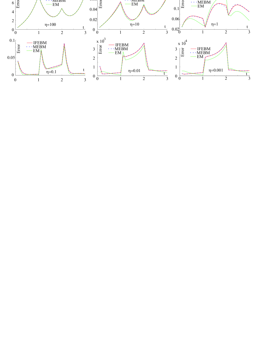
Figure 1: Error graphs for different integrations methods; $\Delta t=0.1$.

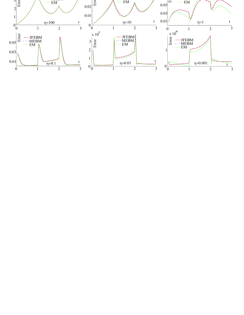
Figure 2: Error graphs for different integrations methods; $\Delta t=0.05$.

Another aspect is the symmetry of the consistent tangent operator $\frac{\displaystyle\partial\ {}^{n+1}\tilde{\mathbf{T}}}{\displaystyle\partial\ {}^{n+1}\mathbf{C}}$. In the current study the tangent is computed by numerical differentiation using the central difference scheme, which provides at least ten-digit accuracy. For computations, the relevant tensors are represented by the 6-vectors as follows (cf. the Voigt notation)

$$\overrightarrow{\mathbf{T}}:=({}^{n+1}\tilde{\mathbf{T}}_{11},{}^{n+1}\tilde{\mathbf{T}}_{22},{}^{n+1}\tilde{\mathbf{T}}_{33},{}^{n+1}\tilde{\mathbf{T}}_{12},{}^{n+1}\tilde{\mathbf{T}}_{13},{}^{n+1}\tilde{\mathbf{T}}_{23}),$$ (59)

$$\overrightarrow{\mathbf{C}}:=({}^{n+1}\mathbf{C}_{11},{}^{n+1}\mathbf{C}_{22},{}^{n+1}\mathbf{C}_{33},2\ {}^{n+1}\mathbf{C}_{12},2\ {}^{n+1}\mathbf{C}_{13},2\ {}^{n+1}\mathbf{C}_{23}).$$ (60)

The deviation of the tangent from the symmetry is measured by the following normalized quantity

$$\text{Deviation}:=\max_{t\in[0,3]}\Big{\|}\frac{\displaystyle\partial\ \overrightarrow{\mathbf{T}}}{\displaystyle\partial\ \overrightarrow{\mathbf{C}}}-\Big{(}\frac{\displaystyle\partial\ \overrightarrow{\mathbf{T}}}{\displaystyle\partial\ \overrightarrow{\mathbf{C}}}\Big{)}^{\text{T}}\Big{\|}\Big{/}\max_{t\in[0,3]}\Big{\|}\frac{\displaystyle\partial\ \overrightarrow{\mathbf{T}}}{\displaystyle\partial\ \overrightarrow{\mathbf{C}}}\Big{\|},\quad\|M\|:=\Big{(}\sum^{6}_{i,j=1}M^{2}_{ij}\Big{)}^{1/2}.$$ (61)

The computed deviation of the consistent tangent from the symmetry is summarized in Table 3 for IFEBM and in Table 4 for 2IEBM. As can be seen from the table, IFEBM provides a tangent which is close to a symmetric one. For the 2IEBM the deviation from the symmetry is barely detectable. Thus, 2IEBM can be used in applications, where the symmetry of the tangent becomes crucial.

Table 3: IFEBM: deviation of the consistent tangent operator from the symmetry.

	$\eta=100$	$\eta=10$	$\eta=1$	$\eta=0.1$	$\eta=0.01$	$\eta=0.001$
$\Delta t=0.1$	$<10^{-9}$	$8.5\cdot 10^{-7}$	$1.8\cdot 10^{-4}$	$8.5\cdot 10^{-5}$	$6.0\cdot 10^{-7}$	$<10^{-9}$
$\Delta t=0.05$	$<10^{-9}$	$1.1\cdot 10^{-7}$	$3.0\cdot 10^{-5}$	$2.7\cdot 10^{-5}$	$4.9\cdot 10^{-7}$	$<10^{-9}$

Table 4: 2IEBM: deviation of the consistent tangent operator from the symmetry.

	$\eta=100$	$\eta=10$	$\eta=1$	$\eta=0.1$	$\eta=0.01$	$\eta=0.001$
$\Delta t=0.1$	$<10^{-9}$	$<10^{-9}$	$<10^{-9}$	$1.2\cdot 10^{-9}$	$<10^{-9}$	$<10^{-9}$
$\Delta t=0.05$	$<10^{-9}$	$<10^{-9}$	$<10^{-9}$	$<10^{-9}$	$<10^{-9}$	$<10^{-9}$

Remark 4
A popular way to enforce the symmetry of the tangent operator exploits the variational nature of the underlying constitutive equations [9, 2, 57]. However, iterative procedures are used in these references.

Remark 5
In a number of FEM applications, the symmetry of the tangent operator is not important. These applications include globally explicit FEM procedures (the stiffness matrix is not assembled at all), geometrically nonlinear computations with follower loads or computations with nonlinear kinematic hardening (the stiffness matrix is a priory non symmetric). Moreover, numerical tests from Section 4.3 show that the global convergence of the FEM procedure with artificially symmetrized tangent is still very good.

4.2 Uniaxial compression tests

In this subsection we consider a composite model with one equilibrium branch and four Maxwell branches connected in parallel. The free energy of the equilibrium branch is given by

$$\rho_{\scriptscriptstyle\text{R}}\psi_{\text{eq}}(\mathbf{C})=\frac{c^{(\text{eq})}_{10}}{2}\big{(}\text{tr}\overline{\mathbf{C}}-3\big{)}+\frac{c^{(\text{eq})}_{01}}{2}\big{(}\text{tr}\overline{\mathbf{C}}-3\big{)}+\frac{k}{50}\big{(}(\text{det}\mathbf{C})^{5/2}+(\text{det}\mathbf{C})^{-5/2}-2\big{)}.$$ (62)

The volumetric part appearing in (62) is taken from [16]; $k$ is the bulk modulus. For the m-th Maxwell branch we put

$$\rho_{\scriptscriptstyle\text{R}}\psi_{\text{ov},m}(\hat{\mathbf{C}}^{(m)}_{\text{e}})=\frac{c^{(m)}_{10}}{2}\big{(}\text{tr}\overline{\hat{\mathbf{C}}^{(m)}_{\text{e}}}-3\big{)}+\frac{c^{(m)}_{01}}{2}\big{(}\text{tr}\overline{(\hat{\mathbf{C}}^{(m)}_{\text{e}})^{-1}}-3\big{)},\ m=1,2,3,4.$$ (63)

For the composite model, the 2nd Piola-Kirchhoff stress equals

$$\tilde{\mathbf{T}}=\tilde{\mathbf{T}}_{\text{eq}}+\sum\limits_{m=1}^{4}\tilde{\mathbf{T}}_{\text{ov},m},\quad\text{where}$$ (64)

$$\tilde{\mathbf{T}}_{\text{eq}}=\mathbf{C}^{-1}(c^{(\text{eq})}_{10}\overline{\mathbf{C}}-c^{(\text{eq})}_{01}\overline{\mathbf{C}^{-1}})^{\text{D}}+\frac{\displaystyle k}{\displaystyle 10}\ \big{(}(\text{det}\mathbf{C})^{5/2}-(\text{det}\mathbf{C})^{-5/2}\big{)}\ \mathbf{C}^{-1},$$ (65)

$$\tilde{\mathbf{T}}_{\text{ov},m}=\mathbf{C}^{-1}\big{(}c^{(m)}_{10}\overline{\mathbf{C}}(\mathbf{C}^{(m)}_{\text{i}})^{-1}-c^{(m)}_{01}\mathbf{C}^{(m)}_{\text{i}}\overline{\mathbf{C}^{-1}}\big{)}^{\text{D}}.$$ (66)

Analogously to (17), the behaviour of each Maxwell branch is described by

$$\dot{\mathbf{C}}^{(m)}_{\text{i}}=\frac{1}{\eta^{(m)}}\big{(}c^{(m)}_{10}\overline{\mathbf{C}}(\mathbf{C}_{\text{i}}^{(m)})^{-1}-c^{(m)}_{01}\mathbf{C}^{(m)}_{\text{i}}\overline{\mathbf{C}^{-1}}\big{)}^{\text{D}}\mathbf{C}^{(m)}_{\text{i}},\quad\mathbf{C}^{(m)}_{\text{i}}|_{t=0}=\mathbf{1}.$$ (67)

The material parameters corresponding to a cartilaginous temporomandibular joint are taken from [26]; they are summarized in Table 5.

Table 5: Material parameters of a cartilaginous temporomandibular joint [26].

	m =1	m = 2	m =3	m=4	equilibrium
$c_{10}$ [MPa]	0.25	0.25	0.36	1.25	0.2
$c_{01}$ [MPa]	0.25	0.25	0.36	1.25	0.2
$\eta$ [MPa s]	25.0	5.0	0.144	0.005	$\infty$

In this subsection we visualize the stress response of the joint tissue subjected to a non-monotonic volume-preserving uniaxial loading. Here, the material is assumed to be incompressible. The strain-controlled loading is given by

$$\mathbf{F}(t)=(1+\varepsilon(t))\mathbf{e}_{1}\otimes\mathbf{e}_{1}+(1+\varepsilon(t))^{-1/2}(\mathbf{e}_{2}\otimes\mathbf{e}_{2}+\mathbf{e}_{3}\otimes\mathbf{e}_{3}),$$ (68)

where $\varepsilon$ stands for the prescribed engineering strain. Three different oscillation frequencies are analyzed (10 Hz, 1 Hz, and 0.1 Hz). For each frequency, two different tests are simulated: one test with the strain amplitude 0.2 and another one with the strain amplitude 0.4. Within each test, the absolute strain rate is constant: $|\dot{\varepsilon}|=const$. The simulation results are shown in Figure 3. The figure reveals that for different loading frequencies IFEBM is sufficiently accurate, even when working with moderate time steps.

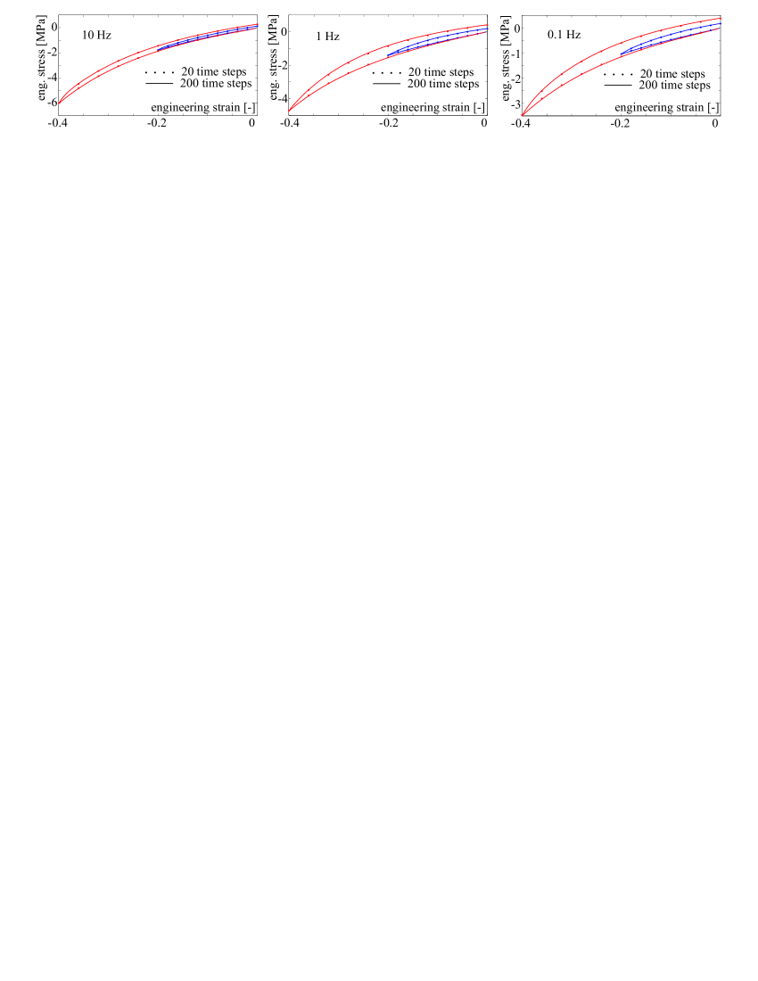
Figure 3: IFEBM-based simulations of a non-monotonic compression test with different strain amplitudes and frequencies.

4.3 Solution of a boundary value problem

In order to demonstrate the applicability of the IFEBM, a representative initial boundary value problem is solved here. The composite material model (65)–(67) introduced in the previous subsection is implemented into the commercial FEM code MSC.MARC via the Hypela2 user interface. The material parameters correspond to the cartilaginous temporomandibular joint (cf. Table 5) with the bulk modulus $k=20$ MPa.

A non-monotonic force-controlled loading is applied to the Cook membrane (Figure 4). The membrane is discretized using 213 elements with quadratic approximation of geometry and displacements; full integration is used. Let $T_{\text{total}}$ be the overall process time. For $t\in[0,T_{\text{total}}/3]$ the applied load increases from zero to the maximum of $0.27$ N; after that the load linearly decreases to $-0.27$ N. Three different loading rates are analyzed, leading to different process durations: $T_{\text{total}}=0.3$ s, $T_{\text{total}}=3$ s, and $T_{\text{total}}=30$ s. The deformed shapes are shown in Figure 4 for $T_{\text{total}}=30$ at different time instances.

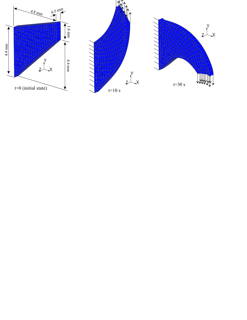
Figure 4: Force-controlled loading of the Cook membrane. Left: specimen’s geometry and dimensions. Middle and right: boundary conditions and deformed configurations at different instances of time.

Constant time steps are implemented in each simulation; simulations with small and large time steps are carried out. A strict convergence criterion is used at each time step: for convergence, the relative error in force and displacements should not exceed 0.01. Two types of computations are carried out: with a general non-symmetric stiffness matrix and with an artificially symmetrized stiffness matrix. The symmetrized version allows us to use a symmetric matrix solver, which is more efficient. Although the consistent tangent operator for IFEBM is not exactly symmetric, the artificial symmetrization did not affect the number of the global equilibrium iterations: MSC.MARC required the same number of iterations, both with symmetric and non-symmetric matrix solvers. The required number of iterations is listed in Table 6. More iterations are needed for the slow process.

Table 6: Number of global equilibrium iterations.

	$T_{\text{total}}=0.3$ s	$T_{\text{total}}=3$ s	$T_{\text{total}}=30$ s
150 steps	449	448	480
15 steps	58	70	131

The simulated force-displacement curves are shown in Figure 5. Although the stress response is history-dependent, simulations with only 15 steps provide sufficiently accurate results. The maximum displacement increases with decreasing loading rate. Thus, the large number of the global equilibrium iterations for the slow process can be explained by pronounced geometric nonlinearities.

Figure 5: Simulated force-displacement curves for three processes with different durations.

5 Discussion and conclusion

A popular version of the finite strain Maxwell fluid is considered, which is based on the multiplicative decomposition of the deformation gradient, combined with hyperelastic relations between stresses and elastic strains. A new iteration free method is proposed for the implicit time stepping, provided that the elastic potential is of the Mooney-Rivlin type.

The following properties of the exact solution are inherited by the proposed IFEBM:

• ${}^{n+1}\mathbf{C}_{\text{i}}$ is symmetric and unimodular: ${}^{n+1}\mathbf{C}_{\text{i}}\in Sym$, $\det({}^{n+1}\mathbf{C}_{\text{i}})=1$,

• ${}^{n+1}\mathbf{C}_{\text{i}}$ is positive definite: ${}^{n+1}\mathbf{C}_{\text{i}}>0$,

• ${}^{n+1}\mathbf{C}_{\text{i}}$ is a smooth function of $\Delta t$,

• complete stress relaxation: ${}^{n+1}\mathbf{C}_{\text{i}}\rightarrow{}^{n+1}\overline{\mathbf{C}}$ as $\Delta t\rightarrow\infty$,

• w-invariance under volume-preserving changes of the reference configuration.

For IFEBM, the consistent tangent operator is nearly symmetric. A slight modification, called 2IEBM, allows one to obtain a tangent operator which is even closer to the set of symmetric fourth-rank tensors. In terms of accuracy, the IFEBM is equivalent to the existing methods like the Euler backward method with exact incompressibility of the flow (MEBM) and the exponential method (EM), but the new method is superior in terms of robustness and computational efficiency.

Since the considered multiplicative Maxwell fluid is widespread in the phenomenological material modelling, the new method can become a method of choice in many applications, especially in those that require increased robustness and efficiency.

Acknowledgements This research was supported by the Russian Science Foundation (project number 15-11-20013).

Appendix A: alternative Eulerian formulation of the model

Let us consider an alternative formulation of the finite strain Maxwell model from Section 2. For simplicity, only incompressible behaviour is analyzed here. Consider the velocity gradient $\mathbf{L}$, the continuum spin $\mathbf{W}$ and the strain rate $\mathbf{D}$

$$\mathbf{L}:=\dot{\mathbf{F}}\mathbf{F}^{-1},\quad\mathbf{W}:=(\mathbf{L}-\mathbf{L}^{\text{T}})/2,\quad\mathbf{D}:=(\mathbf{L}+\mathbf{L}^{\text{T}})/2.$$ (69)

The formulation is based on the additive decomposition of the strain rate tensor $\mathbf{D}$ into the elastic part $\mathbf{D}_{\text{e}}$ and the inelastic part $\mathbf{D}_{\text{i}}$

$$\mathbf{D}=\mathbf{D}_{\text{e}}+\mathbf{D}_{\text{i}}.$$ (70)

Following [6], assume that $\mathbf{X}_{\text{e}}$ is a symmetric positive definite tensor with $\det(\mathbf{X}_{\text{e}})=1$; $\mathbf{X}_{\text{e}}$ operates on the current configuration. Let the free energy per unit mass be given by the isotropic function $\psi(\mathbf{X}_{\text{e}})$. Assume that the Kirchhoff stress $\mathbf{S}$ is computed through

$$\mathbf{S}=2\rho_{\scriptscriptstyle\text{R}}\frac{\displaystyle\partial\psi(\mathbf{X}_{\text{e}})}{\displaystyle\partial\mathbf{X}_{\text{e}}}\mathbf{X}_{\text{e}}.$$ (71)

The flow rule is postulated on the current configuration

$$\mathbf{D}_{\text{i}}=\frac{1}{2\eta}\mathbf{S}^{\text{D}}.$$ (72)

Moreover, the evolution of $\mathbf{X}_{\text{e}}$ is described by (cf. [6])

$$\mathbf{X}^{ZJ}_{\text{e}}=\mathbf{D}_{\text{e}}\ \mathbf{X}_{\text{e}}+\mathbf{X}_{\text{e}}\ \mathbf{D}_{\text{e}},\quad\text{where}\quad\mathbf{X}^{ZJ}_{\text{e}}:=\dot{\mathbf{X}}_{\text{e}}+\mathbf{X}_{\text{e}}\ \mathbf{W}-\mathbf{W}\ \mathbf{X}_{\text{e}}.$$ (73)

Let us show that this model is equivalent to (26)-(27). First, combining (70) and (73), we arrive at

$$\dot{\mathbf{X}}_{\text{e}}+\mathbf{X}_{\text{e}}\ \mathbf{W}-\mathbf{W}\ \mathbf{X}_{\text{e}}=(\mathbf{D}-\mathbf{D}_{\text{i}})\mathbf{X}_{\text{e}}+\mathbf{X}_{\text{e}}(\mathbf{D}-\mathbf{D}_{\text{i}}).$$ (74)

Next, substituting (72) into this, we obtain after some rearrangements

$$\dot{\mathbf{X}}_{\text{e}}-\mathbf{X}_{\text{e}}\ \mathbf{L}^{\text{T}}-\mathbf{L}\ \mathbf{X}_{\text{e}}=-\frac{1}{2\eta}(\mathbf{S}^{\text{D}}\mathbf{X}_{\text{e}}+\mathbf{X}_{\text{e}}\mathbf{S}^{\text{D}}).$$ (75)

Relation (71) implies that $\mathbf{X}_{\text{e}}$ and $\mathbf{S}^{\text{D}}$ commute. Post-multiplying both sides of (75) with $\mathbf{X}^{-1}_{\text{e}}$ and recalling the definition of the Lie derivative (25), we obtain

$$\text{\calligra{L}}_{v}(\mathbf{X}_{\text{e}})\mathbf{X}^{-1}_{\text{e}}=-\frac{1}{\eta}\mathbf{S}^{\text{D}}.$$ (76)

It remains to note that (70) and (76) become identical to (26)-(27), if $\mathbf{X}_{\text{e}}$ is formally replaced by $\mathbf{B}_{\text{e}}$. Thus, we are dealing with two different Eulerian formulations of the same model.

Appendix B: estimation of $\varphi$

Here we estimate the unknown $\varphi$; the derivation is similar to that presented in Appendix C of [52]. The equation $\varphi\ \mathbf{X}=\mathbf{A}-\varepsilon\mathbf{X}^{2}$ yields $\mathbf{X}$ as an implicit function of $\varphi$ and $\varepsilon$. Its expansion in Taylor series for small $\varepsilon$ is as follows

$$\mathbf{X}=\tilde{\mathbf{X}}(\varphi,\varepsilon)=\frac{1}{\varphi}\mathbf{A}-\frac{\varepsilon}{\varphi^{3}}{\mathbf{A}}^{2}+O(\varepsilon^{2}),\quad\mathbf{X}|_{\varepsilon=0}=\frac{1}{\varphi}\mathbf{A}.$$ (77)

The unknown $\varphi$ is estimated using the incompressibility relation $\det(\textbf{X})=1$, which yields

$$\varphi=\tilde{\varphi}(\varepsilon),\quad\varphi_{0}:=\tilde{\varphi}(0)=(\det\mathbf{A})^{1/3}.$$ (78)

Using the implicit function theorem, we have

$$\frac{d\tilde{\varphi}(\varepsilon)}{d\varepsilon}|_{\varepsilon=0}=-\frac{\partial\det\tilde{\mathbf{X}}(\varphi,\varepsilon)}{\partial\varepsilon}|_{\varphi=\varphi_{0},\varepsilon=0}\ \Big{(}\frac{\partial\det\tilde{\mathbf{X}}(\varphi,\varepsilon)}{\partial\varphi}|_{\varphi=\varphi_{0},\varepsilon=0}\Big{)}^{-1}.$$ (79)

Differentiating expansion $\eqref{AppendixB3}_{1}$, we obtain

$$\frac{\partial\det\tilde{\mathbf{X}}(\varphi,\varepsilon)}{\partial\varepsilon}|_{\varphi=\varphi_{0},\varepsilon=0}=\det\tilde{\mathbf{X}}(\varphi_{0},0)\ (\tilde{\mathbf{X}}(\varphi_{0},0))^{-1}:\Big{(}-\frac{\mathbf{A}^{2}}{\varphi_{0}^{3}}\Big{)},$$ (80)

$$\frac{\partial\det\tilde{\mathbf{X}}(\varphi,\varepsilon)}{\partial\varphi}|_{\varphi=\varphi_{0},\varepsilon=0}=\det\tilde{\mathbf{X}}(\varphi_{0},0)\ (\tilde{\mathbf{X}}(\varphi_{0},0))^{-1}:\Big{(}-\frac{\mathbf{A}}{\varphi_{0}^{2}}\Big{)}.$$ (81)

Substituting this into (79), we obtain

$$\frac{d\tilde{\varphi}(\varepsilon)}{d\varepsilon}|_{\varepsilon=0}=-\frac{\text{tr}\mathbf{A}}{3\varphi_{0}},\quad\tilde{\varphi}(\varepsilon)=\varphi_{0}-\frac{\text{tr}\mathbf{A}}{3\varphi_{0}}\varepsilon+O(\varepsilon^{2}).$$ (82)

Interestingly, this estimation is exact in the case of isotropic $\mathbf{A}$. Moreover, a higher-order approximation of $\varphi$ is possible. However, the higher-order approximation would be even less accurate dealing with finite $\varepsilon$, which may occur in practice.

Appendix C: order of approximation

Let us show that IFEBM is first order accurate. Toward that end we consider a typical time interval $(t_{n},t_{n+1})$; ${}^{n+1}\mathbf{C}$ and ${}^{n}\mathbf{C}_{\text{i}}$ are given and $\det{}^{n}\mathbf{C}_{\text{i}}=1$. Let $\mathbf{C}^{\text{exact}}_{\text{i}}$ be the exact solution to equation (17) with the initial condition $\mathbf{C}_{\text{i}}|_{t=t_{n}}={}^{n}\mathbf{C}_{\text{i}}$ and $\mathbf{C}\equiv{}^{n+1}\mathbf{C}$; ${}^{n+1}\mathbf{C}^{\text{IFEBM}}_{\text{i}}$ is the corresponding IFEBM-solution. It is sufficient to show that for small $\Delta t$

$${}^{n+1}\mathbf{C}^{\text{IFEBM}}_{\text{i}}-\mathbf{C}^{\text{exact}}_{\text{i}}(t_{n+1})=O((\Delta t)^{2}).$$ (83)

We re-write (17) in the compact form

$$\dot{\mathbf{C}}_{\text{i}}(t)=\mathbf{f}(\mathbf{C}_{\text{i}}(t))\mathbf{C}_{\text{i}},\quad\text{tr}\mathbf{f}\equiv 0.$$ (84)

Since $\mathbf{C}^{\text{exact}}_{\text{i}}(\cdot)$ is smooth, the mean value theorem implies that there exists $t^{*}\in(t_{n},t_{n+1})$ such that

$$\mathbf{C}^{\text{exact}}_{\text{i}}(t_{n+1})={}^{n}\mathbf{C}_{\text{i}}+\Delta t\ \mathbf{f}(\mathbf{C}^{\text{exact}}_{\text{i}}(t^{*}))\mathbf{C}^{\text{exact}}_{\text{i}}(t^{*}).$$ (85)

Due to the smoothness of $\mathbf{f}$, we have

$$\mathbf{C}^{\text{exact}}_{\text{i}}(t_{n+1})={}^{n}\mathbf{C}_{\text{i}}+\Delta t\ \mathbf{f}({}^{n}\mathbf{C}_{\text{i}})\ {}^{n}\mathbf{C}_{\text{i}}+O((\Delta t)^{2}).$$ (86)

Since $\det\mathbf{C}^{\text{exact}}_{\text{i}}(t_{n+1})=1$ and $\det{}^{n}\mathbf{C}_{\text{i}}=1$, using the Jacobi formula we have

$${}^{n}\mathbf{C}^{-1}_{\text{i}}:\big{(}\Delta t\ \mathbf{f}({}^{n}\mathbf{C}_{\text{i}}){}^{n}\mathbf{C}_{\text{i}}+O((\Delta t)^{2})\big{)}=0.$$ (87)

On the other hand, for the exact solution of the discretized equation (30) we have

$${}^{n+1}\mathbf{C}_{\text{i}}={}^{n}\mathbf{C}_{\text{i}}+\Delta t\ \mathbf{f}({}^{n+1}\mathbf{C}_{\text{i}})\ {}^{n+1}\mathbf{C}_{\text{i}}+\tilde{\varphi}\ {}^{n+1}\mathbf{C}_{\text{i}},\quad\det{}^{n+1}\mathbf{C}_{\text{i}}=1.$$ (88)

Due to the smoothness of $\mathbf{f}$,

$${}^{n+1}\mathbf{C}_{\text{i}}={}^{n}\mathbf{C}_{\text{i}}+\Delta t\ \mathbf{f}({}^{n}\mathbf{C}_{\text{i}})\ {}^{n}\mathbf{C}_{\text{i}}+\tilde{\varphi}\ {}^{n}\mathbf{C}_{\text{i}}+O((\Delta t)^{2}).$$ (89)

Similarly to (87), using the incompressibility condition $\det{}^{n+1}\mathbf{C}_{\text{i}}=1$, we obtain

$${}^{n}\mathbf{C}^{-1}_{\text{i}}:\big{(}\Delta t\ \mathbf{f}({}^{n}\mathbf{C}_{\text{i}}){}^{n}\mathbf{C}_{\text{i}}+\tilde{\varphi}\ {}^{n}\mathbf{C}_{\text{i}}+O((\Delta t)^{2})\big{)}=0.$$ (90)

Subtracting (87) from (90), we conclude that $\tilde{\varphi}=O((\Delta t)^{2})$. Having this in mind and subtracting (86) from (89), we obtain the desired estimation

$${}^{n+1}\mathbf{C}_{\text{i}}-\mathbf{C}^{\text{exact}}_{\text{i}}(t_{n+1})=\tilde{\varphi}+O((\Delta t)^{2})=O((\Delta t)^{2}).$$ (91)

Note that the IFEBM solution differs slightly from ${}^{n+1}\mathbf{C}_{\text{i}}$, since in EFEBM the parameter $\varphi$ is not identified exactly, but estimated using equation (37). The error in the estimation of $\varphi$ is of order $O(\varepsilon^{2})=O((\Delta t)^{2})$. Thus, the corresponding $\tilde{\varphi}$ is still $O((\Delta t)^{2})$ and (91) is still valid:

$${}^{n+1}\mathbf{C}^{*}_{\text{i}}-\mathbf{C}^{\text{exact}}_{\text{i}}(t_{n+1})=O((\Delta t)^{2}).$$ (92)

Finally, the projection $\overline{(\cdot)}$ (cf. (39)) brings changes which are only $O((\Delta t)^{2})$: ${}^{n+1}\mathbf{C}^{*}_{\text{i}}-\overline{{}^{n+1}\mathbf{C}^{*}_{\text{i}}}=O((\Delta t)^{2})$ (cf. Appendix B in [50]). Thus, IFEBM is first order accurate.

Appendix D: exact preservation of the w-invariance

A general definition of the w-invariance under isochoric change of the reference configuration is presented in [44]. In a simple formulation, the w-invariance of a material model says that for any volume-preserving change of the reference configuration there is a transformation of initial conditions ensuring that the predicted Cauchy stresses are not affected by the reference change. The w-invariance represents a generalized symmetry of the constitutive equations indicating that the analyzed material exhibits fluid-like properties.

In the particular case of constitutive equations (12) and (16), the w-invariance property is formulated in the following way. Let $\mathbf{F}_{0}$ be arbitrary second-rank tensor, such that $\det\mathbf{F}_{0}=1$. Consider a prescribed history of the right Cauchy-Green tensor $\mathbf{C}(t)$, $t\in[0,T]$ and the initial condition $\mathbf{C}_{\text{i}}|_{t=0}=\mathbf{C}_{\text{i}}^{0}$. Let $\mathbf{C}^{\text{new}}_{\text{i}}$ be a new solution of (12), (16) corresponding to the new loading programm $\mathbf{C}^{\text{new}}(t)$ and new initial conditions

$$\mathbf{C}^{\text{new}}(t):=\mathbf{F}^{-\text{T}}_{0}\mathbf{C}(t)\mathbf{F}^{-1}_{0},\quad\mathbf{C}^{\text{new}}_{\text{i}}|_{t=0}=\mathbf{F}^{-\text{T}}_{0}\mathbf{C}_{\text{i}}^{0}\mathbf{F}^{-1}_{0}.$$ (93)

System (12), (16) is w-invariant if and only if the original and new solutions a related through

$$\mathbf{C}^{\text{new}}_{\text{i}}(t)=\mathbf{F}^{-\text{T}}_{0}\mathbf{C}_{\text{i}}(t)\mathbf{F}^{-1}_{0}.$$ (94)

Let ${}^{n+1}\mathbf{C}$, ${}^{n}\mathbf{C}_{\text{i}}$, and $\mathbf{F}_{0}$ be given. Denote by ${}^{n+1}\mathbf{C}_{\text{i}}$ and ${}^{n+1}\mathbf{C}^{\text{new}}_{\text{i}}$ the IFEBM-solutions pertaining to the original and new inputs, respectively:

$$\big{(}^{n+1}\mathbf{C},^{n}\mathbf{C}_{\text{i}}\big{)}\ \stackrel{{\scriptstyle\text{IFEBM}}}{{\mapsto}}\ {}^{n+1}\mathbf{C}_{\text{i}},\quad\big{(}\mathbf{F}^{-\text{T}}_{0}\ {}^{n+1}\mathbf{C}\ \mathbf{F}^{-1}_{0},\mathbf{F}^{-\text{T}}_{0}\ {}^{n}\mathbf{C}_{\text{i}}\ \mathbf{F}^{-1}_{0}\big{)}\ \stackrel{{\scriptstyle\text{IFEBM}}}{{\mapsto}}\ ^{n+1}\mathbf{C}^{\text{new}}_{\text{i}}$$ (95)

In analogy to the continuous case (94), the algorithm is said to preserve the w-invariance if

$${}^{n+1}\mathbf{C}^{\text{new}}_{\text{i}}=\mathbf{F}^{-\text{T}}_{0}\ {}^{n+1}\mathbf{C}^{\text{new}}_{\text{i}}\ \mathbf{F}^{-1}_{0}.$$ (96)

Algorithms satisfying (96) are advantageous over algorithms which violate this symmetry restriction (cf. the discussion in [50]). A straightforward (but tedious) way of proving (96) is to substitute the IFEBM equations into (96) and to check the identity. A more elegant proof is based on the observation that the IFEBM on the reference configuration (cf. table 1) is equivalent to the IFEBM on the current configuration (cf. table 2). More precisely, let ${}^{n+1}\mathbf{F}$ be any second-rank tensor, such that ${}^{n+1}\mathbf{F}^{\text{T}}\ {}^{n+1}\mathbf{F}={}^{n+1}\mathbf{C}$. Recall that, according to (50) and (54), ${}^{n+1}{\mathbf{B}}_{\text{e}}$ is a unique function of the trial value ${}^{n+1}{\mathbf{B}}^{\text{trial}}_{\text{e}}$. The following computation steps yield exactly the IFEBM-solution:

$${}^{n+1}{\mathbf{B}}^{\text{trial}}_{\text{e}}={}^{n+1}{\mathbf{F}}\ {}^{n}\mathbf{C}^{-1}_{\text{i}}\ {}^{n+1}{\mathbf{F}}^{\text{T}},\quad{}^{n+1}{\mathbf{B}}^{\text{trial}}_{\text{e}}\stackrel{{\scriptstyle\eqref{Eulerian3},\eqref{Eulerian5}}}{{\mapsto}}{}^{n+1}{\mathbf{B}}_{\text{e}},\quad{}^{n+1}\mathbf{C}_{\text{i}}={}^{n+1}{\mathbf{F}}^{\text{T}}\ {}^{n+1}{\mathbf{B}}^{-1}_{\text{e}}\ {}^{n+1}{\mathbf{F}}.$$ (97)

Now, for the new inputs ${}^{n+1}\mathbf{C}^{\text{new}}=\mathbf{F}^{-\text{T}}_{0}\ {}^{n+1}\mathbf{C}\ \mathbf{F}^{-1}_{0}$ and ${}^{n}\mathbf{C}^{\text{new}}_{\text{i}}=\mathbf{F}^{-\text{T}}_{0}\ {}^{n}\mathbf{C}_{\text{i}}\ \mathbf{F}^{-1}_{0}$ we may put ${}^{n+1}\mathbf{F}^{\text{new}}={}^{n+1}\mathbf{F}\mathbf{F}^{-1}_{0}$. Then

$$({}^{n+1}{\mathbf{B}}^{\text{trial}}_{\text{e}})^{\text{new}}={}^{n+1}{\mathbf{F}}^{\text{new}}\ ({}^{n}\mathbf{C}^{\text{new}}_{\text{i}})^{-1}\ ({}^{n+1}{\mathbf{F}}^{\text{new}})^{\text{T}}={}^{n+1}{\mathbf{B}}^{\text{trial}}_{\text{e}}.$$ (98)

Since the trial values for the original and new inputs coincide, we have

$${}^{n+1}{\mathbf{B}}^{\text{new}}_{\text{e}}={}^{n+1}{\mathbf{B}}_{\text{e}},\quad{}^{n+1}\mathbf{C}^{\text{new}}_{\text{i}}=({}^{n+1}{\mathbf{F}}^{\text{new}})^{\text{T}}\ {}^{n+1}{\mathbf{B}}^{-1}_{\text{e}}\ {}^{n+1}{\mathbf{F}}^{\text{new}}=\mathbf{F}^{-\text{T}}_{0}\ {}^{n+1}\mathbf{C}_{\text{i}}\ \mathbf{F}^{-1}_{0}.$$ (99)

That is exactly the required relation between ${}^{n+1}\mathbf{C}^{\text{new}}_{\text{i}}$ and ${}^{n+1}\mathbf{C}_{\text{i}}$. In the same way, the w-invariance can be proved for the 2IEBM.

Appendix E: MEBM and EM

We consider the initial value problem

$$\dot{\mathbf{C}_{\text{i}}}(t)=\mathbf{f}(\mathbf{C}_{\text{i}}(t),t)\mathbf{C}_{\text{i}}(t),\quad\mathbf{C}_{\text{i}}(0)=\mathbf{C}_{\text{i}}^{0},\quad\det(\mathbf{C}_{\text{i}}^{0})=1,\quad\text{where}\ \text{tr}\mathbf{f}\equiv 0.$$

Assume that ${}^{n}\mathbf{C}_{\text{i}}$ is known. The classical Euler Backward method (EBM) is based on the equation

$${}^{n+1}\mathbf{C}_{\text{i}}^{\text{EBM}}={}^{n}\mathbf{C}_{\text{i}}+\Delta t\ \mathbf{f}({}^{n+1}\mathbf{C}_{\text{i}}^{\text{EBM}},t_{n+1})\ {}^{n+1}\mathbf{C}_{\text{i}}^{\text{EBM}}.$$ (100)

In the current study we use its modification, called modified Euler backward method (MEBM), which guaranties that $\det(\mathbf{}^{n+1}\mathbf{C}_{\text{i}})=1$

$${}^{n+1}\mathbf{C}_{\text{i}}^{\text{MEBM}}=\overline{{}^{n}\mathbf{C}_{\text{i}}+\Delta t\mathbf{f}({}^{n+1}\mathbf{C}_{\text{i}}^{\text{MEBM}},t_{n+1})\ {}^{n+1}\mathbf{C}_{\text{i}}^{\text{MEBM}}}.$$ (101)

Another modification of the Euler backward method was presented in [19], also to enforce the inelastic incompressibility. The exponential method (EM) corresponds to the equation

$${}^{n+1}\mathbf{C}_{\text{i}}^{\text{EM}}=\exp\big{(}\displaystyle\Delta t\ \mathbf{f}({}^{n+1}\mathbf{C}_{\text{i}}^{\text{EM}},t_{n+1})\big{)}\ {}^{n}\mathbf{C}_{\text{i}}.$$ (102)

MEBM and EM exactly preserve the geometric property (19): ${}^{n+1}\mathbf{C}_{\text{i}}\in Sym$, $\det({}^{n+1}\mathbf{C}_{\text{i}})=1$.

References

- [1] Balan C, Tsakmakis C. A finite deformation formulation of the 3-parameter viscoelastic fluid. Journal of non-newtonian fluid mechanics 2002;103(1):45–64.
- [2] Bleier N, Mosler J. Efficient variational constitutive updates by means of a novel parameterization of the flow rule. Int. J. Numer. Meth. Engng 2012;89:1120–1143.
- [3] Buechler MA, Luscher DJ. A semi-implicit integration scheme for a combined viscoelastic-damage model of plastic bonded explosives. Int. J. Numer. Meth. Engng 2014;99(1):54–78.
- [4] Dettmer W, Reese S. On the theoretical and numerical modelling of Armstrong -Frederick kinematic hardening in the finite strain regime. Computer Methods in Applied Mechanics and Engineering 2004;193:87 -116.
- [5] Diani J, Gilormini P, Fredy C, Rousseau I. Predicting thermal shape memory of crosslinked polymer 362 networks from linear viscoelasticity. Int. J. of Soli. and Struct. 2012;49(5):793 799.
- [6] Donner H, Ihlemann J, A numerical framework for rheological models based on the decomposition of the deformation rate tensor. Proc. Appl. Math. Mech. 2016;16:319–320.
- [7] Eidel B, Kuhn C. Order reduction in computational inelasticity: Why it happens and how to overcome it – The ODE-case of viscoelasticity. International Journal for Numerical Methods in Engineering 2011;87:1046–1073.
- [8] Eidel B, Stumpf F, Schröder J, Finite strain viscoelasticity: how to consistently couple discretizations in time and space on quadrature-point level for full order and a considerable speed-up. Computational Mechanics 2013;52(3):463–483.
- [9] Fancello EA, Ponthot JP, Stainier L. A variational formulation of constitutive models and updates in non-linear finite viscoelasticity. International Journal for Numerical Methods in Engineering 2006;65(11):1831 1864.
- [10] Feigenbaum HP, Dugdale J, Dafalias YF, Kourousis KI, Plesek J, Multiaxial ratcheting with advanced kinematic and directional distortional hardening rules. International Journal of Solids and Structures 2012;49:3063–3076.
- [11] Gasser TC, Forsell C. The numerical implementation of invariant-based viscoelastic formulations at finite strains. An anisotropic model for the passive myocardium. Computer Methods in Applied Mechanics and Engineering 2011;200:3637–3645.
- [12] Ghobadi E, Sivanesapillai R, Musialak J, Steeb H. Modeling based characterization of thermorheological properties of polyurethane ESTANE. International Journal of Polymer Science 2016;2016 Article ID 7514974, 11 pages http://dx.doi.org/10.1155/2016/7514974
- [13] Haider J, Lee CH, Gil AJ, Bonet J, A first-order hyperbolic framework for large strain computational solid dynamics: An upwind cell centred Total Lagrangian scheme. Journal for Numerical Methods in Engineering 2017;109(3):407–456.
- [14] Hartmann S. Finite-Elemente Berechnung inelastischer Kontinua. Interpretation als Algebro-Differentialgleichungssysteme. Habilitation thesis, Kassel, 2003.
- [15] Hartmann S, Hamkar AW. Rosenbrock-type methods applied to finite element computations within finite strain viscoelasticity. Computer Methods in Applied Mechanics and Engineering 2010;199:1455–1470.
- [16] Hartmann S, Neff P. Polyconvexity of generalized polynomial-type hyperelastic strain energy functions for near-incompressibility. International Journal of Solids and Structures 2003;40:2767–2791.
- [17] Hasanpour K, Ziaei-Rad S, Mahzoon M. A large deformation framework for compressible viscoelastic materials: Constitutive equations and finite element implementation. International Journal of Plasticity 2009;25:1154–1176.
- [18] Helm D. Formgedächtnislegierungen, experimentelle Untersuchung, phänomenologische Modellierung und numerische Simulation der thermomechanischen Materialeigenschaften, Universitätsbibliothek Kassel, 2001.
- [19] Helm D. Stress computation in finite thermoviscoplasticity. International Journal of Plasticity 2006;22:1699–1721.
- [20] Helm D. Thermomechanics of martensitic phase transitions in shape memory alloys I, constitutive theories for small and large deformations. J. Mech. Mater. Struct. 2007;2(1):87–112.
- [21] Holmes DW, Loughran JG. Numerical aspects associated with the implementation of a finite strain, elasto-viscoelastic-viscoplastic constitutive theory in principal stretches. Int. J. Numer. Meth. Engng. 2010;83:366–402.
- [22] Holzapfel GA, Gasser TC, Stadler M, A structural model for the viscoelastic behavior of arterial walls: Continuum formulation and finite element analysis. European Journal of Mechanics A/Solids 2002;21:441–463.
- [23] Huber N, Tsakmakis C. Finite deformation viscoelasticity laws. Mechanics of Materials 2000;32:1–18.
- [24] Johlitz M, Dippel B, Lion A. Dissipative heating of elastomers: a new modelling approach based on finite and coupled thermomechanics. Continuum Mechanics and Thermodynamics 2016;28(4):1111–1125.
- [25] Kleuter B, Menzel A, Steinmann P. Generalized parameter identification for finite viscoelasticity. Computer Methods in Applied Mechanics and Engineering 2007;196:3315–3334.
- [26] Koolstra JH, Tanaka E, Van Eijden TMGJ. Viscoelastic material model for the temporomandibular joint disc derived from dynamic shear tests or strain-relaxation tests. Journal of Biomechanics 2007;40:2330–2334.
- [27] Landgraf R, Shutov AV, Ihlemann J. Efficient time integration in multiplicative inelasticity. Proc. Appl. Math. Mech. 2015;15:325–326
- [28] Lion A. Constitutive modelling in finite thermoviscoplasticity: a physical approach based on nonlinear rheological elements. International Journal of Plasticity 2000;16:469–494.
- [29] Latorre M, Montáns FJ. A new class of plastic flow evolution equations for anisotropic multiplicative elastoplasticity based on the notion of a corrector elastic strain rate, arXiv:1701.00095v1 (2016)
- [30] Lejeunes S, Boukamel A, Méo S. Finite element implementation of nearly-incompressible rheological models based on multiplicative decompositions. Computers and Structures 2011;89:411–421.
- [31] Lion A. A physically based method to represent the thermo-mechanical behaviour of elastomers. Acta Mechanica 1997;123:1–25.
- [32] Misra S, Ramesh KT, Okamura AM, Modeling of tool-tissue interactions for computer-based surgical simulation: a literature review. Presence: Teleoperators and Virtual Environments 2008;17(5):463–491.
- [33] Nedjar B. Frameworks for finite strain viscoelastic-plasticity based on multiplicative decompositions. Part I: Continuum formulations. Comput. Methods Appl. Mech. Engrg. 2002;191:1541–1562.
- [34] Peric D, Crook AJL. Computational strategies for predictive geology with reference to salt tectonics. Comput. Methods Appl. Mech. Engrg. 2004;193:5195–5222
- [35] Ram D, Gast T, Jiang C, Schroeder C, Stomakhin A, Teran J, Kavehpour P. A material point method for viscoelastic fluids, foams and sponges. Proceedings of the 14th ACM SIGGRAPH/Eurographics Symposium on Computer Animation 2015:157–163.
- [36] Rauchs G. Finite element implementation including sensitivity analysis of a simple finite strain viscoelastic constitutive law. Computers and Structures 2010;88:825–836.
- [37] Reese S. Thermomechanische Modellierung gummiartiger Polymerstrukturen. Habilitation thesis, Hannover, 2000.
- [38] Reese S, Govindjee S. A theory of finite viscoelasticity and numerical aspects. International Journal of Solids and Structures 1998;35:3455–3482.
- [39] Reiner M. Deformation, Strain and Flow. An Elementary Introduction to Rheology, 2nd edition, 1960.
- [40] Schüler T, Jänicke R, Steeb H, Nonlinear modeling and computational homogenization of asphalt concrete on the basis of XRCT scans. Construction and Building Materials 2016;109:96 108.
- [41] Silbermann CB, Shutov AV, Ihlemann J. On operator split technique for the time integration within finite strain viscoplasticity in explicit FEM. Proc. Appl. Math. Mech. 2014;14:355–356.
- [42] Simo JC, Meschke G. A new class of algorithms for classical plasticity extended to finite strains. Application to geomaterials. Computational mechanics 1993;11(4):253–278.
- [43] Shutov AV, Kreißig R. Application of a coordinate-free tensor formalism to the numerical implementation of a material model. ZAMM 2008;88(11):888–909.
- [44] Shutov AV, Ihlemann J. Analysis of some basic approaches to finite strain elasto-plasticity in view of reference change. International Journal of Plasticity 2014;63:183–197.
- [45] Shutov AV. Seven different ways to model viscoelasticity in a geometrically exact setting. Proceedings of the 7th European Congress on Computational Methods in Applied Sciences and Engineering 2016;1, 1959–1970.
- [46] Shutov AV, Kreißig R. Geometric integrators for multiplicative viscoplasticity: analysis of error accumulation. Computer Methods in Applied Mechanics and Engineering 2010;199:700–711.
- [47] Shutov AV, Kuprin C, Ihlemann J, Wagner MFX, Silbermann C. Experimentelle Untersuchung und numerische Simulation des inkrementellen Umformverhaltens von Stahl 42CrMo4. Mat.-wiss. u.Werkstofftech. 2010;41(9):765–775.
- [48] Shutov AV, Panhans S, Kreißig R, A phenomenological model of finite strain viscoplasticity with distortional hardening. ZAMM 2011;91(8):653–680.
- [49] Shutov AV, Ihlemann J. A viscoplasticity model with an enhanced control of the yield surface distortion. International Journal of Plasticity 2012;39:152–167.
- [50] Shutov AV, Landgraf R, Ihlemann J. An explicit solution for implicit time stepping in multiplicative finite strain viscoelasticity. Computer Methods in Applied Mechanics and Engineering 2013;256:213–225.
- [51] Shutov AV, Silbermann CB, Ihlemann J. Ductile damage model for metal forming simulations including refined description of void nucleation. International Journal of Plasticity 2015;71:195-217.
- [52] Shutov AV. Efficient implicit integration for finite-strain viscoplasticity with a nested multiplicative split. Computer Methods in Applied Mechanics and Engineering 2016;306(1):151–174.
- [53] Shutov AV, Larichkin AYu, Shutov VA. Modelling of cyclic creep in the finite strain range using a nested split of the deformation gradient. ZAMM (2017), DOI: 10.1002/zamm.201600286
- [54] Sidoroff F, Un modèle viscoélastique non linéaire avec configuration intermédiaire. J Mécanique 1974;13(4):679–713.
- [55] Simo JC, Algorithms for static and dynamic multiplicative plasticity that preserve the classical return mapping schemes of the infinitesimal theory. Computer Methods in Applied Mechanics and Engineering 1992;99:61–112.
- [56] Simo JC, Miehe C. Associative coupled thermoplasticity at finite strains: formulation, numerical analysis and implementation. Computer Methods in Applied Mechanics and Engineering 1992;98:41–104.
- [57] Vassoler JM, Stainier L, Fancello E. A variational framework for fiber-reinforced viscoelastic soft tissues including damage. Int. J. Numer. Meth. Engng (2016) DOI: 10.1002/nme.5236
- [58] Vladimirov I, Pietryga M, Reese S. On the modelling of non-linear kinematic hardening at finite strains with application to springback – Comparison of time integration algorithms. Int. J. Numer. Meth. Engng 2008;75:1–28.