LHC Run I Bounds on Minimal Lepton Flavour Violation in Type–III See–saw: A Case Study

Abstract

We study the bounds on minimal lepton flavour violation in the context of Type-III see–saw imposed by LHC Run I search for events which contain two charged leptons (either electron or muons of equal or opposite sign), two jets from a hadronically decaying $W$ boson and large missing transverse momentum. In this scenario the flavour structure of the couplings of the triplet fermions to the Standard Model leptons can be reconstructed from the neutrino mass matrix and lepton number violation is very suppressed. We find that using the information on charge and flavour of the leptons in the above final state it is possible to unambiguously rule out this scenario with triplet masses lighter than 300 GeV at 95% CL. The same analysis allows to exclude triplet masses masses up to 480 GeV at 95% CL for normal ordering of neutrino masses and specific values of a Majorana CP phase currently undetermined by neutrino physics.

1 Introduction

Massive neutrinos are our first and only undoubted evidence of physics beyond the Standard Model (SM). The evidence arises from a variety of neutrino experiments which have detected the effect of their mass via the flavour oscillation of neutrinos with energies ranging between tens of keV and tens of GeV GonzalezGarcia:2007ib . The obvious question that this observation raises is that of the dynamics of the New Physics (NP) responsible for the neutrino mass.

It is well known that in the framework of effective operators for NP there is just one dimension-five operator which can be built Weinberg:1979sa , ${\cal O}=\alpha_{5}/\Lambda_{LN}\,L_{L}L_{L}HH$, where $L_{L}$ and $H$ are the leptonic and Higgs $SU(2)_{L}$ doublets. This operator breaks total lepton number and after electroweak symmetry breaking it generates Majorana masses for the neutrinos $m_{\nu}\sim\alpha_{5}v^{2}/\Lambda_{LN}$, where $v$ is the SM Higgs vacuum expectation value (vev). This explains the lightness of the neutrino mass due to the large scale of total lepton number violation $\Lambda_{LN}$. In the simplest UV completions, this dimension-5 operator can be generated by the tree-level exchange of three types of new states: lepton singlets in the Type–I see-saw scenarios Minkowski:1977sc ; Yanagida:1979as ; GellMann:1980vs ; Mohapatra:1979ia , a scalar triplet for the Type–II mechanisms Konetschny:1977bn ; Cheng:1980qt ; Lazarides:1980nt ; Schechter:1980gr ; Mohapatra:1980yp , and lepton triplets for Type–III models Foot:1988aq . In any of these mechanisms the smallness of the neutrino mass can be naturally explained with Yukawa couplings $\lambda\sim{\cal O}(1)$ if the masses of the new states are $M\sim\Lambda_{LN}\sim 10^{14-15}$ GeV. Notwithstanding consistent models of lower scale see–saw exist in the literature for some time; see e.g. Mohapatra:1986bd ; Kersten:2007vk ; Chen:2011de .

Given the energy range of the neutrino experiments it is clear that if the NP scale is beyond $\sim$ GeV it is not possible to clarify its origin within the oscillation neutrino experiments themselves. On the other hand, the high energy frontier is currently being explored by the CERN Large Hadron Collider (LHC) which has been running for eight years with a reach to NP at the TeV scale. So far no clear evidence of NP has been observed at LHC which bears implications for models constructed to explain the neutrino masses containing new states at the TeV scale.

Generically the expected event rates at LHC in neutrino mass models depend not only on the mass and weak charge of the new states involved, but also on the flavour structure of their couplings which determines their decay modes. A priory, the decay channels are arbitrary in most Type–I and Type–III see–saw models, making difficult to derive unambiguous constraints on the NP scale in these scenarios delAguila:2008cj ; Aguilar-Saavedra:2013twa . For example searches for triplet leptons of the Type–III see–saw models have been performed both by CMS CMS:2012ra ; CMS:2017wua ; CMS:2016hmk ; CMS:2015mza and ATLAS Aad:2015cxa ; ATLAS:2013hma collaborations, however, most of these searches have been carried out within the context of simplified models such as Ref. Biggio:2011ja and the derived bounds can be evaded depending on which is the dominant decay mode of the triplet leptons.

One exception are see–saw models which extend the principle of minimal flavour violation to the leptonic sector. Minimal flavour violation was first introduced for quarks Chivukula:1987py ; Buras:2000dm ; DAmbrosio:2002vsn as a way to explain the absence of NP effects in flavour changing processes in meson decays. The basic assumption is that the only source of flavour mixing in the full theory is the same as in the SM, i.e. the quark Yukawa couplings. This idea was latter on extended for leptons Cirigliano:2005ck ; Davidson:2006bd and in particular to TeV scale see–saw models Cirigliano:2005ck ; Davidson:2006bd ; Gavela:2009cd ; Alonso:2011jd .

From the point of view of LHC phenomenology minimal lepton flavour violation (MLFV) see–saw models are attractive since, a) the new states can be light enough to be produced at LHC, and b) their signatures are fully determined by the neutrino parameters. As discussed in Ref. Gavela:2009cd scalar (Type-II) see–saw with light doublet-triplet mixing is a light scale MLFV model by construction (for early study of their observability see for example  Perez:2008ha ; Garayoa:2007fw ). In Ref. Gavela:2009cd simple MLFV models for fermionic see–saw were also presented. In Type–I see–saw the new states are singlets under the SM gauge group, and therefore, they can only be produced via their mixing with the SM neutrinos. This leads to small production rates which makes the model only marginally testable at LHC. Type-III see–saw fermions, on the contrary, are $SU(2)_{L}$ triplets with weak-interaction pair-production cross section, and consequently, having the potential to allow for tests of the hypothesis of MLFV.

In Ref. Eboli:2011ia we studied the potential of LHC to unravel the existence of triplet fermionic states that appear in MLFV Type-III see–saw models of neutrino mass. Here, we obtain the bounds on the NP scale of this scenario that originates from the ATLAS Aad:2015cxa searches in the final state topology containing two charged leptons (electrons and/or muons), two jets compatible with a hadronically decaying $W$ and missing transverse momentum. This ATLAS analysis is best suited for testing the MLFV scenario because it classifies the final states in the different flavour and charge combinations, allowing to fully exploit the predictions of the MLFV Type-III see–saw model. We find that using this ATLAS data it is possible to unambiguously rule out the MLFV Type–III see–saw scenario with triplet masses lighter than 300 GeV at 95% CL irrespective of the neutrino mass ordering and other unknowns in the light neutrino sector, in particular of the so–far undetermined Majorana CP violating phase. The same analysis allows to rule out triplet masses masses up to 480 GeV at 95% CL for normal order (NO) scenarios and specific values of that phase.

This paper is organized as follows. We first summarize in Sec. 2 the basics of the MLFV Type-II see–saw model and we quantify the allowed range of the relevant couplings controlling the triplet decay modes as derived from the present analysis of neutrino oscillation data from Ref. Esteban:2016qun . Section  3 describes our simulation of signal events by the reaction $pp\rightarrow ll^{\prime}jj\nu\nu$ with $l^{(\prime)}=e$ or $\mu$ in the context of the MLFV Type-III see–saw model. The quantification of the bounds is presented in Sec. 4. In doing so we have put special emphasis and we have quantified how the information on flavour and charge information of the produced leptons is important for maximal sensitivity to MLFV.

2 MLFV Type–III see–saw model

In Ref. Eboli:2011ia we introduced the simplest MLFV Type-III see–saw model which was adapted from the Type-I one presented in Ref. Gavela:2009cd . For completeness we summarize here its main features.

The particle contents of model is that of the SM extended with two fermion triplets $\vec{\Sigma}=\left(\Sigma_{1},\Sigma_{2},\Sigma_{3}\right)$ and $\vec{\Sigma}^{\prime}=\left(\Sigma^{\prime}_{1},\Sigma^{\prime}_{2},\Sigma^{\prime}_{3}\right)$, each one formed by three right-handed Weyl spinors of zero hypercharge. Hence, the Lagrangian is

$${\mathcal{L}}={\mathcal{L}}_{SM}+{\mathcal{L}}_{K}+{\mathcal{L}}_{Y}+{\mathcal{L}}_{\Lambda}$$ (1)

with

$${\mathcal{L}}_{K}= i\left(\overline{\vec{\Sigma}}/\!\!\!\!D_{\mu}\vec{\Sigma}+\overline{\vec{\Sigma}^{\prime}}/\!\!\!\!D_{\mu}\vec{\Sigma}^{\prime}\right)\;,$$ (2)

$${\mathcal{L}}_{Y}= -Y_{i}^{\dagger}\overline{L^{w}_{Li}}\left(\vec{\Sigma}\cdot\vec{\tau}\right)\tilde{\phi}-\epsilon Y_{i}^{\prime{\dagger}}\overline{L^{w}_{Li}}\left(\vec{\Sigma}^{\prime}\cdot\vec{\tau}\right)\tilde{\phi}+h.c.\;,$$ (3)

$${\mathcal{L}}_{\Lambda}= -\frac{\Lambda}{2}\left(\overline{\vec{\Sigma}^{c}}\vec{\Sigma}^{\prime}+\overline{\vec{\Sigma}^{\prime c}}\vec{\Sigma}\right)-\frac{\mu}{2}\overline{\vec{\Sigma}^{\prime c}}\vec{\Sigma}^{\prime}-\frac{\mu^{\prime}}{2}\overline{\vec{\Sigma}^{c}}\vec{\Sigma}+h.c.\;.$$ (4)

Here $\vec{\tau}$ are the Pauli matrices, the gauge covariant derivative is defined as $D_{\mu}=\partial_{\mu}+ig\vec{T}\cdot\vec{W}_{\mu}$, where $\vec{T}$ are the three-dimensional representation of the $SU(2)_{L}$ generators, $\phi$ stands for the SM Higgs doublet field, and $L^{w}_{i}=(\nu^{w}_{i},\ell^{w}_{i})^{T}$ are the three weak eigenstate lepton doublets of the SM. The parameters $\epsilon$, $\mu$ and $\mu^{\prime}$ are flavour-blind and small, i.e., the scales $\mu$ and $\mu^{\prime}$ are much smaller than $\Lambda$ and $v$ while $\epsilon\ll 1$.

The Lagrangian in Eq. (1) breaks total lepton number due to the simultaneous presence of the Yukawa terms $Y_{i}$ and $\epsilon Y^{\prime}_{i}$ as well as to the existence of the $\mu$ and $\mu^{\prime}$ terms. Thus in the limit $\mu,\mu^{\prime},\epsilon\rightarrow 0$ it is possible to define a conserved total lepton number by assigning $L(L^{w})=L(\Sigma)=-L(\Sigma^{\prime})=1$. Without any loss of generality one can work in a basis in which $\Lambda$ is real while both $Y$ and $Y^{\prime}$ are complex. In general the parameters $\mu$ and $\mu^{\prime}$ would be complex, but for the sake of simplicity we take them to be real in what follows though it is straight forward to generalize the expression to include the relevant phases Abada:2007ux .

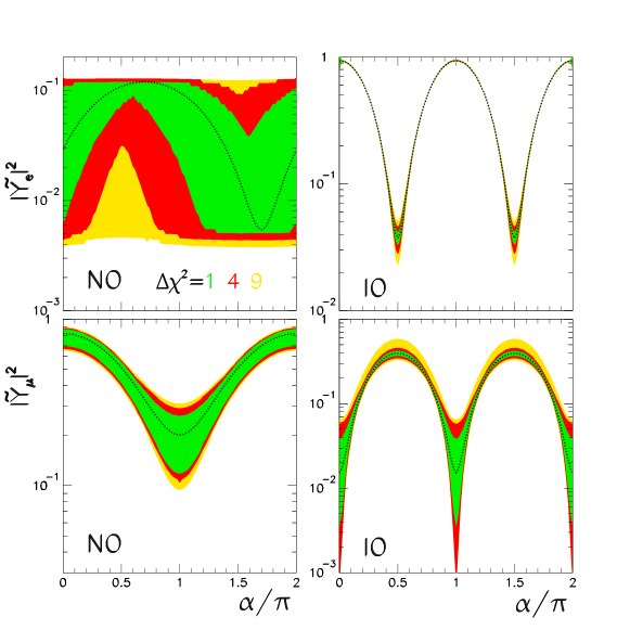
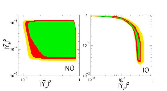
Figure 1: Allowed ranges of the Yukawa couplings $|\tilde{Y}_{e}|^{2}\equiv|Y_{1}|^{2}/y^{2}$ and $|\tilde{Y}_{\mu}|^{2}\equiv|Y_{2}|^{2}/y^{2}$ obtained from the global analysis of neutrino data in Ref. Esteban:2016qun . The upper four panel shows the values of the couplings as a function of the unknown Majorana phase $\alpha$. The correlation between the two couplings is shown in the two lower panels. The left (right) panels correspond to normal (inverted) ordering. The dotted line corresponds to the best fit values. The ranges in the filled green, red and yellow areas are shown at 1$\sigma$, $2\sigma$, and 3$\sigma$ with 1 dof ($\Delta\chi^{2}=1,4,9$ respectively).

After electroweak symmetry breaking, in the unitary gauge, the leptonic mass matrices are

$${\mathcal{L}}_{m} = -\frac{1}{2}\left(\overline{\vec{\nu^{w}_{L}}^{c}}\ \overline{\tilde{N}_{R}}\ \overline{\tilde{N}_{R}^{\prime}}\right)M_{0}\left(\begin{array}[]{c}\vec{\nu^{w}_{L}}\\ \tilde{N}_{R}^{c}\\ \tilde{N}_{R}^{\prime c}\end{array}\right)-\left(\overline{\vec{\ell^{w}_{L}}}\ \overline{E_{L}}\ \overline{E_{L}^{\prime}}\right)M_{\pm}\left(\begin{array}[]{c}\vec{\ell^{w}_{R}}\\ E_{R}\\ E_{R}^{\prime}\end{array}\right)+h.c.$$ (11)

with

$$M_{0}=\left(\begin{array}[]{ccc}0&\frac{v}{\sqrt{2}}Y^{T}&\epsilon\frac{v}{\sqrt{2}}Y^{\prime T}\\ \frac{v}{\sqrt{2}}Y&\mu^{\prime}&\Lambda\\ \epsilon\frac{v}{\sqrt{2}}Y^{\prime}&\Lambda&\mu\end{array}\right) \;\;\;\;\hbox{ and }\;\;\;\;M_{\pm}=\left(\begin{array}[]{ccc}\frac{v}{\sqrt{2}}Y^{\ell}&vY^{\dagger}&\epsilon vY^{\prime\dagger}\\ 0&\mu^{\prime}&\Lambda\\ 0&\Lambda&\mu\end{array}\right)\;,$$ (18)

where $Y^{\ell}$ are the charged lepton Yukawa couplings of the SM. $\vec{\nu}^{w}$ and $\vec{\ell}^{w}$ are column vectors containing respectively the three neutrinos and charged leptons of the SM in the weak basis. The charge eigenstates Dirac fermions $E$ and $E^{\prime}$ and the neutral Majorana fermions $\tilde{N}$ and $\tilde{N}^{\prime}$ are defined in terms of the triplet states, $\Sigma^{(\prime)}_{\pm}=\frac{1}{\sqrt{2}}\left(\Sigma^{(\prime)}_{1}\mp i\Sigma^{(\prime)}_{2}\right)$, and $\Sigma^{(\prime)}_{0}=\Sigma^{(\prime)}_{3}$, as

$$E^{(\prime)}=\Sigma^{(\prime)}_{-}+{\Sigma_{+}^{(\prime)}}^{c} \;\;\;\;\tilde{N}^{(\prime)}=\Sigma^{(\prime)}_{0}+{\Sigma^{(\prime)}_{0}}^{c}\;.$$ (19)

The mass basis is composed of:

• Three light Majorana neutrinos $\nu_{i}$ (with the lightest one being massless) and three light charged leptons leptons $\ell_{i}$ with masses

  $$m^{diag}_{\nu} = {V^{\nu}}^{T}\left[-\frac{v^{2}}{2\Lambda}\epsilon\left[\left(Y^{\prime}-\frac{1}{\epsilon}\frac{\mu}{2\Lambda}Y\right)^{T}Y+Y^{T}\left(Y^{\prime}-\frac{1}{\epsilon}\frac{\mu}{2\Lambda}Y\right)\right]\right]V^{\nu}\;,$$ (20)

  $$m^{diag}_{\ell} = \frac{v}{\sqrt{2}}{V^{\ell}}^{\dagger}_{R}Y^{\ell\dagger}\left[1-\frac{v^{2}}{2\Lambda^{2}}Y^{\dagger}Y\right]V^{\ell}_{L}\;,$$ (21)

  where $V^{\nu}$ and $V^{\ell}_{L,R}$ being $3\times 3$ unitary matrices and in general, one can choose the flavour basis such that $V^{\ell}_{L}=V^{\ell}_{R}=I$.

• Two charged heavy leptons, $E_{1}^{-}$ and $E_{2}^{+}$, both with masses $M\simeq\Lambda(1\mp\frac{\mu+\mu^{\prime}}{2\Lambda})$.

• Two heavy Majorana neutral leptons and two charged heavy leptons also with masses $M\simeq\Lambda(1\mp\frac{\mu+\mu^{\prime}}{2\Lambda})$ with which we build a quasi-Dirac heavy state $N$.

The relation between the weak and mass eigenstate to first order in the small parameters $\mu$, $\mu^{\prime}$ and $\epsilon$ is:

$$\nu_{L}^{w} = V^{\nu}\nu_{L}+\frac{v}{\sqrt{2}\Lambda}Y^{\dagger}N_{L}+\frac{v}{\sqrt{2}\Lambda}\left(\epsilon Y^{\prime\dagger}-\left(\frac{3\mu+\mu^{\prime}}{4\Lambda}\right)Y^{\dagger}\right)N_{R}^{c}\;,$$ (22)

$$\ell^{w}_{L} = \ell_{L}+\frac{v}{\Lambda}Y^{\dagger}E_{1L}^{-}+\frac{v}{\Lambda}\left(\epsilon Y^{\prime\dagger}-\left(\frac{3\mu+\mu^{\prime}}{4\Lambda}\right)Y^{\dagger}\right)E_{2R}^{+c}\;,$$ (23)

$$\ell^{w}_{R} = \ell_{R}\;,$$ (24)

$$\tilde{N}_{L} = N_{R}^{c}-\left(\frac{\mu-\mu^{\prime}}{4\Lambda}\right)N_{L}-\frac{v}{\sqrt{2}\Lambda}\left(\epsilon Y^{\prime}-\frac{\mu}{\Lambda}Y\right)V^{\nu}\nu_{L}\;,$$ (25)

$$\tilde{N}^{\prime}_{L} = N_{L}+\left(\frac{\mu-\mu^{\prime}}{4\Lambda}\right)N_{R}^{c}-\frac{v}{\sqrt{2}\Lambda}YV^{\nu}\nu_{L}\;,$$ (26)

$$E_{L} = E_{2R}^{+c}-\left(\frac{\mu-\mu^{\prime}}{4\Lambda}\right)E_{1L}^{-}-\frac{v}{\Lambda}\left(\epsilon Y^{\prime}-\frac{\mu}{\Lambda}Y\right)\ell_{L}\;,$$ (27)

$$E_{R} = E_{1R}^{-}-\left(\frac{\mu-\mu^{\prime}}{4\Lambda}\right)E_{2L}^{+c}\;,$$ (28)

$$E^{\prime}_{L} = E_{1L}^{-}+\left(\frac{\mu-\mu^{\prime}}{4\Lambda}\right)E_{2R}^{+c}-\frac{v}{\Lambda}Y\ell_{L}\;,$$ (29)

$$E^{\prime}_{R} = E_{2L}^{+c}+\left(\frac{\mu-\mu^{\prime}}{4\Lambda}\right)E_{1R}^{-}\;.$$ (30)

From the above relations it follows that the neutral weak interactions of the light states take the same form as that on the SM and the charged current interactions involve a 3x3 unitary matrix $U_{LEP}=V^{\nu}$ which after phase redefinition of the light charged leptons, can be chosen

$$\!\!\!\!\!\!\!\!\!\!\!\!\!\!\!\!U_{LEP}= = \begin{pmatrix}1&0&0\\ 0&c_{23}&{s_{23}}\\ 0&-s_{23}&{c_{23}}\end{pmatrix}\!\!\!\begin{pmatrix}c_{13}&0&s_{13}e^{-i\delta_{\text{CP}}}\\ 0&1&0\\ -s_{13}e^{i\delta_{\text{CP}}}&0&c_{13}\end{pmatrix}\!\!\!\begin{pmatrix}c_{21}&s_{12}&0\\ -s_{12}&c_{12}&0\\ 0&0&1\end{pmatrix}\!\!\!\begin{pmatrix}e^{-i\alpha}&0&0\\ 0&e^{i\alpha}&0\\ 0&0&1\end{pmatrix},$$ (31)

where $c_{ij}\equiv\cos\theta_{ij}$ and $s_{ij}\equiv\sin\theta_{ij}$. The angles $\theta_{ij}$ can be taken without loss of generality to lie in the first quadrant, $\theta_{ij}\in[0,\pi/2]$ and the phases $\delta_{\text{CP}},\;\alpha\in[0,2\pi]$. The leptonic mixing matrix contains only one Majorana phase because there are only two heavy triplets and consequently only two light neutrinos are massive while the lightest one remains massless. Also notice that unitarity violation in the charged current and flavour mixing in the neutral current of the light leptons in generated at higher order Schechter:1979bn ; Antusch:2006vwa ; Abada:2007ux .

This model is MLFV because one can fully reconstruct the neutrino Yukawa coupling $Y$ and the combination $\widehat{Y^{\prime}}=Y^{\prime}-\frac{1}{\epsilon}\frac{\mu}{2\Lambda}Y$ from the neutrino mass matrix Gavela:2009cd (up to two real normalization factors $y$ and $\hat{y}^{\prime}$) as follows:

$$\begin{array}[]{c|c}{\rm NO}\;(m_{1}=0<m_{2}<m_{3})&{\rm IO}\;(m_{3}=0<m_{1}<m_{2})\\[8.5359pt] \hline\cr r=\frac{\Delta m^{2}_{21}}{\Delta m^{2}_{32}}&r=-\frac{\Delta m^{2}_{21}}{\Delta m^{2}_{31}}\\[8.5359pt] \rho=\frac{\sqrt{1+r}-\sqrt{r}}{\sqrt{1+r}+\sqrt{r}}&\rho=\frac{\sqrt{1+r}-1}{\sqrt{1+r}+1}\\[8.5359pt] m_{2,3}=\frac{\epsilon y{\widehat{y^{\prime}}}v^{2}}{\Lambda}(1\mp\rho)&m_{1,2}=\frac{\epsilon y{\widehat{y^{\prime}}}v^{2}}{\Lambda}(1\mp\rho)\\[8.5359pt] Y_{a}=\frac{y}{\sqrt{2}}\left(\sqrt{1+\rho}\ U_{a3}^{*}+\sqrt{1-\rho}\ U_{a2}^{*}\right)&Y_{a}=\frac{y}{\sqrt{2}}\left(\sqrt{1+\rho}\ U_{a2}^{*}+\sqrt{1-\rho}\ U_{a1}^{*}\right)\\[8.5359pt] \widehat{Y^{\prime}}_{a}=\frac{\widehat{y^{\prime}}}{\sqrt{2}}\left(\sqrt{1+\rho}\ U_{a3}^{*}-\sqrt{1-\rho}\ U_{a2}^{*}\right)&\widehat{Y^{\prime}}_{a}=\frac{\widehat{y^{\prime}}}{\sqrt{2}}\left(\sqrt{1+\rho}\ U_{a2}^{*}-\sqrt{1-\rho}\ U_{a1}^{*}\right)\\ \end{array}$$ (32)

We plot in Fig. 1 the ranges of the Yukawa couplings $|\tilde{Y}_{e}|^{2}\equiv|Y_{1}|^{2}/y^{2}$ and $|\tilde{Y}_{\mu}|^{2}\equiv|Y_{2}|^{2}/y^{2}$ obtained by projecting the allowed ranges of oscillation parameters from the global analysis of neutrino data Esteban:2016qun using Eqs. (32). In the first and second rows we plot the ranges of the Yukawa couplings as a function of the unknown Majorana phase $\alpha$ while the lower row shows the correlation between the electron and muon Yukawa couplings. This figure illustrates the quite different allowed ranges and correlation of the electron and muon Yukawa couplings in the two orderings. As a curiosity we notice that in NO the dependence of the range of $|Y_{e}|$ on $\alpha$ is driven by the present hint of $\delta_{\rm CP}\sim 270^{\circ}$ in the oscillation data analysis Esteban:2016qun because $\alpha$ enters via ${\rm Re}(U_{e3}U_{e2}^{*})\propto\cos(\alpha+\delta_{\rm CP})$.

In what respects the interactions of the heavy states, as discussed in Ref. Eboli:2011ia , lepton number violating couplings appear due to ${\cal O}(\epsilon,\mu/\Lambda,\mu^{\prime}/\Lambda)$ mixings and mass splittings in the heavy states, that are, by hypothesis, very suppressed in MLFV models. This renders the lepton number violating processes involving heavy fermions unobservable at LHC, at a difference with the non MLFV scenarios for Type–III see–saw for which $\Delta L=2$ final states constitute a smoking gun Franceschini:2008pz ; Bajc:2007zf . Consequently in what follows we concentrate in the lepton conserving interaction Lagrangian with $\Lambda=M$ being the common mass of the heavy states:

$${\mathcal{L}}_{W}= -g\left(\overline{E^{-}_{1}}\gamma^{\mu}NW_{\mu}^{-}-\overline{N}\gamma^{\mu}E^{+}_{2}W_{\mu}^{-}\right)+h.c.$$ (33)

$$-g\left(\frac{1}{\sqrt{2}}K_{a}\overline{\ell_{aL}}\gamma^{\mu}N_{L}W_{\mu}^{-}+\tilde{K}_{a}\overline{\nu_{aL}}\gamma^{\mu}E^{+}_{2L}W_{\mu}^{-}\right)+h.c.$$

$${\mathcal{L}}_{Z}= gC_{W}\left(\overline{E^{-}_{1}}\gamma^{\mu}E^{-}_{1}Z_{\mu}-\overline{E^{+}_{2}}\gamma^{\mu}E^{+}_{2}Z_{\mu}\right)$$ (34)

$$+\frac{g}{2\sqrt{2}C_{W}}\left(\frac{1}{\sqrt{2}}\tilde{K}_{a}\overline{\nu_{aL}}\gamma^{\mu}N_{L}Z_{\mu}+K_{a}\overline{\ell_{aL}}\gamma^{\mu}E^{-}_{1L}Z_{\mu}\right)+h.c.$$

$${\mathcal{L}}_{\gamma}= e\left(\overline{E^{-}_{1}}\gamma^{\mu}E^{-}_{1}A_{\mu}-\overline{E^{+}_{2}}\gamma^{\mu}E^{+}_{2}A_{\mu}\right)$$ (35)

$${\mathcal{L}}_{h^{0}}= \frac{gM}{\sqrt{2}M_{W}}\left(\frac{1}{\sqrt{2}}\tilde{K}_{a}\overline{\nu_{aL}}N_{R}+K_{a}\overline{\ell_{aL}}E^{-}_{1R}\right)+h.c.\;.$$ (36)

where $c_{W}$ stands for the cosine of the weak mixing angle and the lepton number conserving couplings of the heavy triplet fermions are

$$\begin{array}[]{ll}K_{a}=-\frac{v}{\sqrt{2}M}{Y_{a}}^{*}\;\;\;,&\;\;\;\tilde{K}_{a}={U^{*}_{LEP}}_{ca}K_{c}\;,\end{array}$$ (37)

which verify

$$\sum_{a=1}^{3}|K_{a}|^{2}=\sum_{a=1}^{3}|\tilde{K}_{a}|^{2}=\frac{y^{2}v^{2}}{2M^{2}}\;.$$ (38)

Notice that flavour structures of the couplings $K$ and $\tilde{K}$ are fully determined by the low energy neutrino parameters. Their strengths are, however, arbitrary as they are controlled by the normalization factor $yv/M$ while it is the combination $\epsilon y\widehat{y^{\prime}}/M$ what is fixed by the neutrino masses.

From these interactions we can obtain the decay widths of the heavy states delAguila:2008hw :

$$\Gamma\left(N\rightarrow\ell_{a}^{-}W^{+}\right)=\frac{g^{2}}{64\pi}|K_{a}|^{2}\frac{M^{3}}{M_{W}^{2}}\left(1-\frac{M_{W}^{2}}{M^{2}}\right)\left(1+\frac{M_{W}^{2}}{M^{2}}-2\frac{M_{W}^{4}}{M^{4}}\right)\;,$$

$$\Gamma\left(N\rightarrow\nu_{a}Z\right)=\frac{g^{2}}{128\pi c_{w}^{2}}|\tilde{K}_{a}|^{2}\frac{M^{3}}{M_{Z}^{2}}\left(1-\frac{M_{Z}^{2}}{M^{2}}\right)\left(1+\frac{M_{Z}^{2}}{M^{2}}-2\frac{M_{Z}^{4}}{M^{4}}\right)\;,$$

$$\Gamma\left(N\rightarrow\nu_{a}h^{0}\right)=\frac{g^{2}}{128\pi}|\tilde{K}_{a}|^{2}\frac{M^{3}}{M_{W}^{2}}\left(1-\frac{M_{h^{0}}^{2}}{M^{2}}\right)^{2}\;,$$ (39)

$$\Gamma\left(E_{2}^{+}\rightarrow\nu_{a}W^{+}\right)=\frac{g^{2}}{32\pi}|\tilde{K}_{a}|^{2}\frac{M^{3}}{M_{W}^{2}}\left(1-\frac{M_{W}^{2}}{M^{2}}\right)\left(1+\frac{M_{W}^{2}}{M^{2}}-2\frac{M_{W}^{4}}{M^{4}}\right)\;,$$

$$\Gamma\left(E_{1}^{-}\rightarrow\ell_{a}^{-}Z\right)=\frac{g^{2}}{64\pi c_{W}^{2}}|K_{a}|^{2}\frac{M^{3}}{M_{Z}^{2}}\left(1-\frac{M_{Z}^{2}}{M^{2}}\right)\left(1+\frac{M_{Z}^{2}}{M^{2}}-2\frac{M_{Z}^{4}}{M^{4}}\right)\;,$$

$$\Gamma\left(E_{1}^{-}\rightarrow\ell_{a}^{-}h^{0}\right)=\frac{g^{2}}{64\pi}|K_{a}|^{2}\frac{M^{3}}{M_{W}^{2}}\left(1-\frac{M_{h^{0}}^{2}}{M^{2}}\right)^{2}\;.$$

Therefore, using Eq. (38) the total decay widths for the three triplet fermions $F=N,E^{-}_{1},E^{+}_{2}$ are

$$\Gamma_{F}^{\mbox{\tiny TOT}}=\frac{g^{2}M^{3}}{64\pi M_{W}^{2}}\frac{y^{2}v^{2}}{M^{2}}(1+{\cal F}_{F}(M))$$ (40)

where ${\cal F}_{F}(M)\rightarrow 0$ for $M\gg m_{h^{0}},M_{Z},M_{W}$. Consequently, the arbitrary $y$ factor cancels out in the branching ratios. Furthermore the branching ratio in a final state with a charge lepton (neutrino) of flavour $\alpha$ produced in the vertex of the heavy state decay is proportional to $|\tilde{Y}_{\alpha}|^{2}$ ($|(U_{LEP}Y)_{\alpha}|^{2}$) times a kinematic factor depending solely on $M$.

Unlike in a general Type–III see–saw model for which the branching ratio of $N$ or $E^{\pm}_{i}$ into a light lepton of a given flavour can be negligibly small, for the MLFV Type–III see–saw model the branching ratios in the different light lepton flavours are fixed by the neutrino physics and are non-vanishing as can be seen from Fig. 1 and Eqs. (39). This makes the flavour composition of the final states in any decay chain of the heavy leptons to be fully determined given a neutrino mass ordering. Consequently in the narrow width approximation the only free parameters in the model are the mass of the states and the Majorana phase $\alpha$, making the model more unambiguously testable. Conversely, as discussed in Ref. Eboli:2011ia in this MLFV Type-III model the values of the neutrino masses imply a lower bound on the total decay width of the triplet fermions as a consequence of the hierarchy between the $L$-conserving and $L$-violating $y$ and $\epsilon\widehat{y^{\prime}}$ constants. So their decay length is too short to produce a detectable displaced decay vertex signature Aad:2008zzm ; Chatrchyan:2008zzk at difference with other see–saw models Franceschini:2008pz ; Bajc:2007zf ; Perez:2008ha ; Li:2009mw .

In order to simulate the expected signals in this MLFV Type–III see–saw model we have implemented the Lagrangian in Eqs. (33)–(36) using the package FeynRules Christensen:2008py ; Alloul:2013bka . We have made available the corresponding model files at the corresponding URL frwiki .

3 Case study: $pp\rightarrow ll^{\prime}jj\nu\nu$

In order to study the sensitivity of LHC Run I to MLFV Type–III see–saw signatures we will use the event topologies studied by ATLAS in Ref. Aad:2015cxa which contain two charged leptons (either electron or muons), two jets from a hadronically decaying $W$ boson and large missing transverse momentum. ATLAS used these topologies to search for heavy fermions in the context of the simplified Type–III see–saw model as implemented in Ref. Biggio:2011ja . They presented their results as number of events for the six different flavour and charge lepton pair combinations: same sign (SS) and opposite sign (SS) $ee$, $\mu\mu$ and $e\mu$. Using those they obtain bounds on the triplet mass which depend on the decay branching ratio into the different flavours. In particular for triplets decaying mostly into $\tau$’s no bound can be derived.

On the contrary, as stressed in the previous section, in the MLFV scenario the flavour and lepton number of the final states produced in the heavy fermion decay chain is very much constrained. Thus having the final states classified in the different flavour and charge combinations makes the result in Ref. Aad:2015cxa best suited for testing the MLFV scenario as we quantify next.

3.1 Contributing subprocesses

Let us start by listing the possible subprocesses contributing to the different flavour and charge combinations in the MLFV Type–III see–saw model. They all proceed by the production of a pair of heavy triplet states and their subsequent decay. The pair production of the fermion triplets takes place via gauge interactions, and, therefore, it depends exclusively upon the mass of the new states. On the other hand, the branching ratios of these fermions into the final states described in the previous section depend upon the Yukawa couplings $\tilde{Y}_{a}$ which vary in the different subprocesses:

• $p\;p\;\rightarrow\;E_{1}^{-}\;\tilde{N}\,,\quad(\;E_{1}^{-}\;\rightarrow\;l_{a}^{-}\;Z\,,\,Z\;\rightarrow\;\nu\;\nu\;)\quad(\;\tilde{N}\;\rightarrow\;l_{b}^{+}\;W^{-}\,,\,W^{-}\;\rightarrow\;j\;j\;)$:
  Using interactions in (33)–(34) it is easy to show that the production cross section for this process is proportional to $|K_{a}|^{2}\,|K_{b}|^{2}$. Therefore, as discussed in the previous section, in the narrow width approximation the production cross section for this process and its charge conjugated one can be factorized as

  $$\sigma_{1}(M)_{ab}\;|\tilde{Y}_{a}|^{2}\,|\tilde{Y}_{b}|^{2}.$$ (41)

• $p\;p\;\rightarrow\;E_{2}^{+}\;\tilde{N}\,,\;(\;E_{2}^{+}\;\rightarrow\;\nu_{c}\;W^{+}\,,\,W^{+}\;\rightarrow\;j\;j\;)\quad(\;\tilde{N}\;\rightarrow\;l_{a}^{+}\;W^{-}\,,\,W^{-}\;\rightarrow\;l_{b}^{-}\;\nu_{c}\;)$:
  whose production cross section is proportional to $|K_{a}|^{2}|\tilde{K}_{c}|^{2}$. So in the narrow width approximation and after summing over the $\nu_{c}$ flavour using Eq. (38) the cross section for this process and its charge conjugated one can be written as

  $$\sigma_{2a}(M)_{ab}\;|\tilde{Y}_{a}|^{2}\;.$$ (42)

• $p\;p\;\rightarrow\;E_{2}^{+}\;\tilde{N}\,,\;(\;E_{2}^{+}\;\rightarrow\;\nu_{c}\;W^{+}\,,\,W^{+}\;\rightarrow\;l_{b}^{+}\;\nu_{b}\;)\quad(\;\tilde{N}\;\rightarrow\;l_{a}^{+}\;W^{-}\,,\,W^{-}\;\rightarrow\;j\;\;j\;)$:
  and the respective charge conjugate process possess a cross section proportional to $|K_{a}|^{2}|\tilde{K}_{c}|^{2}$. As before, in the narrow width approximation and after summing over the $\nu_{c}$ flavour we parametrize the production cross section as

  $$\sigma_{2b}(M)_{ab}\;|\tilde{Y}_{a}|^{2}\;.$$ (43)

• $p\;p\;\rightarrow\;E_{2}^{+}\;\tilde{N}\,,\quad(\;E_{2}^{+}\;\rightarrow\;\nu_{c}\;W^{+}\,\,,\,\,W^{+}\;\rightarrow\;j\;j\;)\quad(\;\tilde{N}\;\rightarrow\;\nu_{d}\;Z\,,\,Z\;\rightarrow\;l_{a}^{-}\;l_{a}^{+}\;)$:
  and its charge conjugate process with cross section proportional to $|\tilde{K}_{c}|^{2}|\tilde{K}_{d}|^{2}$ that after summing over the neutrino flavours $c$ and $d$ reads

  $$\sigma_{2c}(M)_{aa}\;.$$ (44)

• $p\;p\;\rightarrow\;E_{1}^{+}\;E_{1}^{-}\,,\quad(\;E_{1}^{+}\;\rightarrow\;l_{a}^{+}\;Z\,,\,Z\;\rightarrow\;j\;j\;)\quad(\;E_{1}^{-}\;\rightarrow\;l_{b}^{-}\;Z\,,\,Z\;\rightarrow\;\nu_{c}\;\nu_{c}\;)$  ,
  $p\;p\;\rightarrow\;E_{1}^{+}\;E_{1}^{-}\,,\quad(\;E_{1}^{+}\;\rightarrow\;l_{a}^{+}\;Z\,,\,Z\;\rightarrow\;\nu_{c}\;\nu_{c}\;)\quad(\;E_{1}^{-}\;\rightarrow\;l_{b}^{-}\;Z\,,\,Z\;\rightarrow\;j\;j\;)$ :
  with cross section

  $$\sigma_{3}(M)_{ab}\;|\tilde{Y}_{a}|^{2}|\tilde{Y}_{b}|^{2}\;.$$ (45)

Altogether the cross section of each OS flavour channel is given by:

$$\sigma^{OS}_{ee} \equiv \left[\sigma_{1}(M)_{ee}\,+\,\sigma_{3}(M)_{ee}\right]|\tilde{Y}_{e}|^{4}\,+\,\sigma_{2a}(M)_{ee}|\tilde{Y}_{e}|^{2}+\,\sigma_{2c}(M)_{ee}\;,$$

$$\sigma^{OS}_{e\mu} \equiv \left[\sigma_{1}(M)_{e\mu}\,+\,\sigma_{1}(M)_{\mu e}\,+\,\sigma_{3}(M)_{e\mu}\,+\,\sigma_{3}(M)_{\mu e}\right]|\tilde{Y}_{e}|^{2}|\tilde{Y}_{\mu}|^{2}\,$$ (46)

$$+\,\sigma_{2a}(M)_{e\mu}|\tilde{Y}_{e}|^{2}\,+\,\sigma_{2a}(M)_{\mu e}|\tilde{Y}_{\mu}|^{2}\;,$$

$$\sigma^{OS}_{\mu\,\mu} \equiv \left[\sigma_{1}(M)_{\mu\mu}\,+\,\sigma_{3}(M)_{\mu\mu}\right]|\tilde{Y}_{\mu}|^{4}\,+\,\sigma_{2a}(M)_{\mu\mu}|\tilde{Y}_{\mu}|^{2}\,+\,\sigma_{2c}(M)_{\mu\mu}\;,$$

while for SS lepton final state

$$\sigma^{SS}_{ee} \equiv \sigma_{2b}(M)_{ee}|\tilde{Y}_{e}|^{2}\;,$$

$$\sigma^{SS}_{e\mu} \equiv \sigma_{2b}(M)_{e\mu}|\tilde{Y}_{e}|^{2}+\,\sigma_{2b}(M)_{\mu e}|\tilde{Y}_{\mu}|^{2}\;,$$ (47)

$$\sigma^{SS}_{\mu\mu} \equiv \sigma_{2b}(M)_{\mu\mu}|\tilde{Y}_{\mu}|^{2}\;.$$

3.2 Simulation of the expected event rates

In our analysis, we first simulated the above parton level signal processes with MadGraph 5 Alwall:2014hca . We then used PYTHIA 6.4  Sjostrand:2006za to generate the parton shower and hadronization. Finally we performed a fast detector simulation with DELPHES 3 deFavereau:2013fsa with jets being reconstructed using the anti-$k_{T}$ algorithm with a radius $R=0.4$ with the package FASTJET Cacciari:2011ma .

In order to reproduce the ATLAS event selection corresponding to the searches in Ref. Aad:2015cxa we required that the events contain exactly two leptons (muons and/or electrons), a minimum of two jets and no b-tagged jet. In the case of OS (SS) leptons the leading lepton must have transverse momentum ($p_{T}$) in excess of 100 (70) GeV with the next-to-leading lepton $p_{T}$ larger than 25 (40) GeV. In addition we imposed the invariant mass of the two leptons to be larger than 130 and 90 GeV for OS and SS events respectively. We also demanded the $p_{T}$ of two leading jets to be larger than 60 (40) and 30 (25) GeV for the OS (SS) final state. Moreover, to characterize the presence of a hadronically decaying $W$ in the event the invariant mass of the leading jet pair was required to be between 60 and 100 GeV, and for OS events we require the two leading jets to satisfy $\Delta R_{jj}<2$. Finally, we only selected events presenting missing transverse energy in excess of 110 (100) GeV for OS (SS) events. We implement the above selection in MadAnalysis5 Conte:2012fm .

In order to tune our calculations we first simulated the signal for the Type-III see–saw model of Ref. Biggio:2011ja which is the one used in the ATLAS analysis. By comparing our number of expected events with the ones obtained by ATLAS in Fig. 2 of Aad:2015cxa for the OS and SS final states presenting $ee$, $e\mu$ and $\mu\mu$ pairs, we extract overall multiplicative correction factors for each of these final states such that our fast simulation agrees with the one of ATLAS. To validate our procedure we verified that our tuned Monte Carlo reproduces the missing transverse momentum distribution presented in Fig. 1 of Aad:2015cxa . We then apply these correction factors in the evaluation of the expected number of events of the MLFV type-III see-saw model.

Concerning backgrounds, the dominant contribution comes from the production of dibosons ($WW$,$WZ$,$ZZ$), $Z$ plus jets, top pairs and single top in association with a $W$. In addition there are also background events that stems from misidentification of leptons. In our analysis we directly use the background rates estimated by ATLAS Aad:2015cxa .

Figure 2 depicts the resulting cross section factors $\sigma_{1}$, $\sigma_{2a}$, $\sigma_{2b}$, and $\sigma_{3}$ introduced in Eqs. (41)–(45), for the events passing the selection cuts and after applying the tuning correction factors. The results are shown as a function of the new fermion mass and for the different lepton flavor combinations and a center-of-mass energies of 8 TeV  . From this figure we can see that the four possible leptonic final states ($ee$, $\mu\mu$, $e\mu$, and $\mu e$) have similar cross section factors for masses larger than 300 GeV, however, closer to the threshold the detection and acceptance efficiencies induce differences among the leptonic final states. In the case of $\sigma_{2a}$ both leptons originate from the decay of a single triplet fermion, therefore reducing the acceptance at small masses due to the OS lepton pair invariant mass cut.

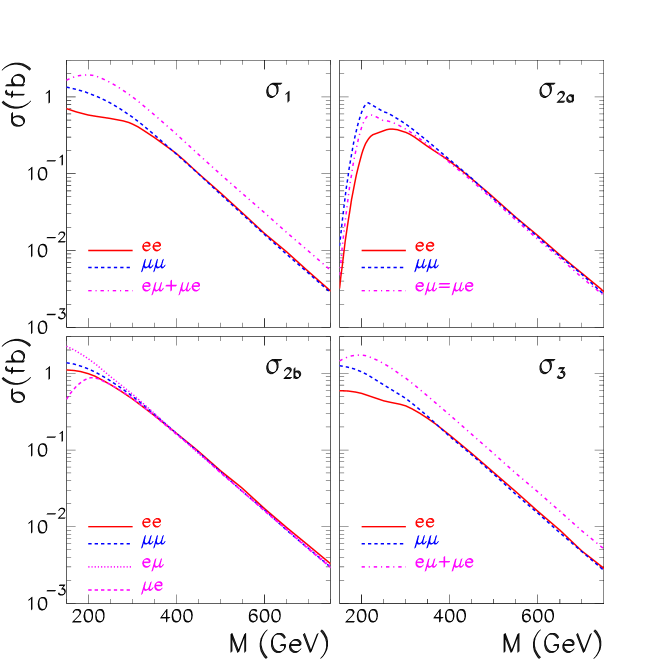
Figure 2: Cross section factors for the different contributions to the event topologies as a function of the triplet mass $M$ as defined in Eqs. (41)–(45) after inclusion of our simulation of the selections of Ref. Aad:2015cxa (see text for details).

Weighting these cross section factors with the different combination of Yukawa couplings as in Eqs. (46) and  (47) and times the luminosity we predict the signal event rates in the different flavour and charge combinations of the final lepton pair. For example in Figs. 3 and  4 we present the event rate prediction as a function of the unknown Majorana phase $\alpha$ for a triplet mass of 300 GeV, an integrated luminosity of 20.3 fb^-1 and normal ordering and inverted ordering respectively. As seen in Fig. 3 for NO, the expected number of $ee$ events is very small for both OS and SS channels. Nevertheless, a considerable number of events containing muons is expected except for $\alpha/\pi$ around 1. This is so because for NO $|\tilde{Y}_{\mu}|$ is much larger than $|\tilde{Y}_{e}|$ as can be seen from Fig. 1. For IO we see in Fig. 4, as could be anticipated from Fig. 1, that the expectations in all flavor channels vary appreciably with the Majorana phase $\alpha$. However, the strong correlation between $|\tilde{Y}_{e}|$ and $|\tilde{Y}_{\mu}|$ in IO – depicted in the right bottom panel of Fig. 1 – guarantees a sizable number of events for almost the entire $\alpha$ range with the signal being dominated by the channels $e\mu$ and $\mu\mu$ for OS leptons and the channel $e\mu$ for SS leptons.

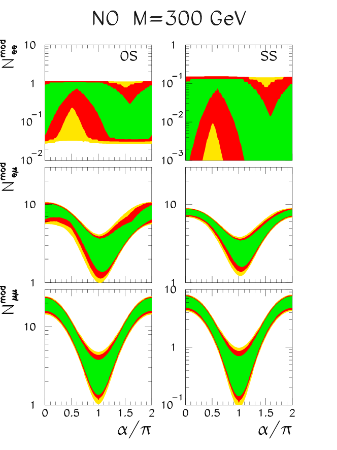
Figure 3: Expected number of signal events at $\sqrt{s}=8$ TeV and an integrated luminosity of 20.3 fb^-1, in each of the six flavour-charge combinations for a triplet mass of $M=300$ GeV and for neutrino parameters corresponding to the NO. The conventions are the same as in Fig.1.

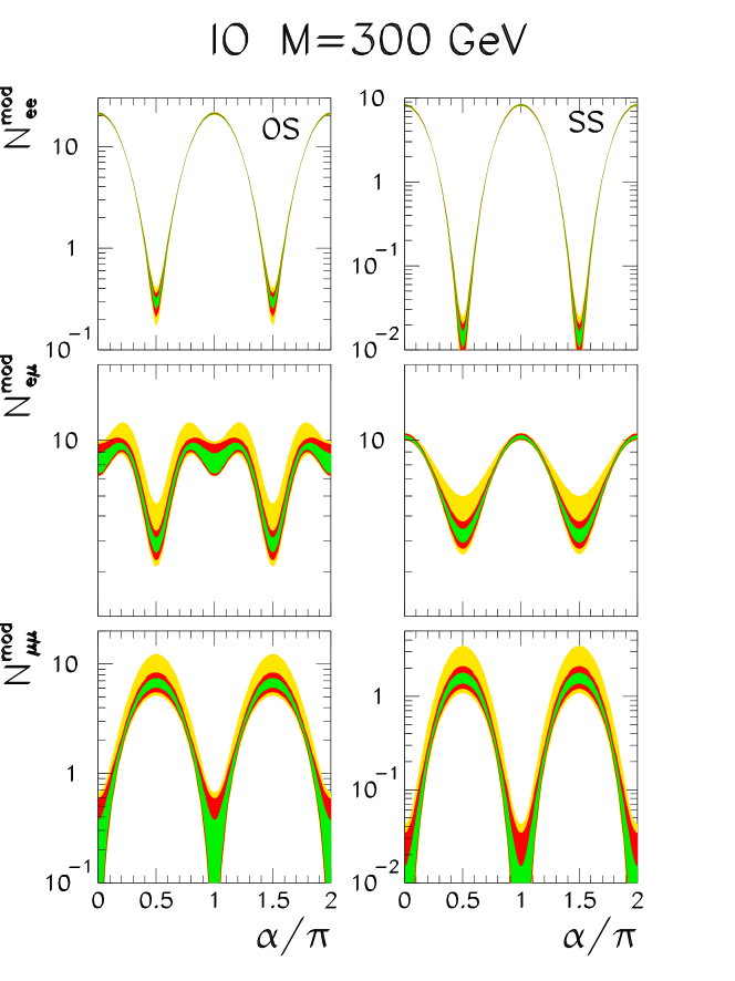
Figure 4: Same as Fig. 4 for IO.

4 Analysis: Results and Discussion

In order to quantify the bounds on the MLFV Type–III see–saw scenario we build the likelihood function using the six data points associated to the events with $ee$, $e\mu$ and $\mu\mu$ leptons of either SS or OS. As discussed in the previous section, we make direct use of the corresponding background estimate by ATLAS which we read from Fig. 2 and Table I of Ref. Aad:2015cxa and that summarize here for completeness:

	OS $ee$	SS $ee$	OS $\mu\mu$	SS $\mu\mu$	OS $e\mu$	SS $e\mu$	total OS	total SS
$N^{dat}$	9	3	3	1	13	0	25	4
$N^{bck}$	$8.5$	$1$	$9.5$	$0.5$	$13$	$1.65$	$31.0\pm 7.7$	$3.15\pm 0.8$

According to Ref. Aad:2015cxa the reported background errors in the table and figure include both the statistical and systematic uncertainties. Comparing the read out of these uncertainties for each of the six individual channels with the total reported in the table we conclude that the $\sim$ 25% background uncertainty is strongly correlated among the different channels as the total background uncertainty comes to be very close to the arithmetic sum of the individual ones, while if they were totally uncorrelated one would expect it to be the quadratic sum.

So we build the likelihood function as

$$-2{\cal L}_{6d}=\chi^{2}_{6d}=\min_{\xi}\left\{2\sum_{i=1,6}\left[(1+\xi)N^{bck}_{i}+N^{mod}_{i}-N^{dat}_{i}\log\frac{N^{dat}_{i}}{(N^{bck}_{i}+N^{mod}_{i})}\right]+\frac{\xi^{2}}{0.25^{2}}\right\}$$ (48)

where we account for the background uncertainty by introducing a unique pull $\xi$ with an uncertainty of 25%. $N^{mod}_{i}$ is the predicted contribution to the number of events in channel $i$ from the triplet production and decays which depends on the triplet mass and the neutrino parameters as discussed in the previous section. In building the likelihood (48) we have used Poisson statistics to account for the small number of events in each channel.

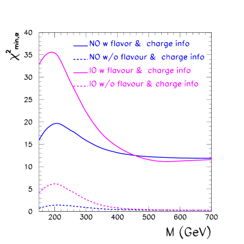
Figure 5: Triplet mass dependence of the $\chi^{2}$ functions of the analysis of $pp\rightarrow ll^{\prime}jj\nu\nu$ events with $l,l^{\prime}$ being either $e$ or $\mu$ of either charge observed in the LHC Run-I in ATLAS Aad:2015cxa when analyzed in the context of MLFV Type–III see–saw model. The full lines correspond to the likelihood function constructed including the full information given on flavour and charge of the final states (see Eq. (48)) while the dashed lines are obtained from the analysis of the total data summing over charge and flavour. The triplet couplings have been marginalized within the ranges allowed at 95% CL by the neutrino oscillation data analysis in Ref. Esteban:2016qun for NO (blue lines) and IO (purple lines) and for any value of the Majorana phase $\alpha$.

We plot as full lines in Fig. 5 the dependence of $\chi^{2}_{6d}$ on the triplet mass after marginalization over the neutrino parameters (including the unknown Majorana phase $\alpha$) over the 95% CL allowed values from the neutrino oscillation analysis for either NO or IO. First thing to notice is that in the SM ($N^{mod}_{i}$=0, which can be inferred from the large M limit in the figure) we find $\chi^{2}_{6d,SM}=11.8$ which is a bit high for 6 data points. This is mostly driven by the OS $\mu\mu$ channel for which 3 events are observed when about 10 are expected in the SM. From this figure we also read that requiring $\chi^{2}_{6d}-\chi^{2}_{6d,SM}<4$ we can infer an absolute bound on the triplet mass of 300 GeV (375 GeV) for NO (IO) light neutrino masses.

In order to stress the importance of the flavour and charge information on the possibility of imposing this bound, we have constructed the corresponding likelihood function summing the information from all the channels. As in this case the total number of observed events is large enough, we assume gaussianity. So we define:

$$\chi^{2}_{tot}=\frac{(N^{tot,bck}+N^{tot,mod}-N^{tot,dat})^{2}}{N^{tot,dat}+(0.25N^{tot,bck})^{2}}\;.$$ (49)

The dependence of $\chi^{2}_{tot}$ on the triplet mass after marginalization over the neutrino parameters (including the unknown Majorana phase $\alpha$) over the 95% CL allowed values from the neutrino oscillation analysis ($\Delta\chi^{2}_{osc}\leq 4$) for either NO or IO is shown as dashed lines in Fig. 5. As the deficit in OS $\mu\mu$ is compensated by the slight excesses in other channels, we find that in this case the SM gives a perfect description of the total observed event rates ($\chi^{2}_{tot,SM}$=0.25). The figure clearly illustrates the relevance of flavour and charge information, as in this case the condition $\chi^{2}_{tot}-\chi^{2}_{tot,SM}<4$ does result into no bound on the triplet mass for NO neutrino masses while it rules out only $M<260$ for IO.

The dependence of the bounds on the unknown phase $\alpha$ is displayed in Fig. 6. The full red regions are excluded values of triplet masses in the MLFV scenario at 95% CL ($\chi^{2}_{6d}-\chi^{2}_{6d,SM}>4$) when marginalizing over the oscillation parameters within the 95% CL allowed values by the oscillation analysis in NO (left) and IO (right) for each value of $\alpha$. The $\alpha$ marginalized bound discussed above correspond to the lightest allowed masses in these panels which for NO ($M>300$ GeV) correspond to $\alpha=\pi$ while for $\alpha=0$, $2\pi$ the bound strengthens to $M>480$ GeV. For IO the dependence of the bound on $\alpha$ is weaker. The marginalized bound $M>380$ GeV corresponds to $\alpha\sim 3\pi/4,3\pi/2$ but it is close to that value for almost all values of alpha. The strongest bound of $M>430$ GeV corresponds also to $\alpha=0$, $2\pi$.

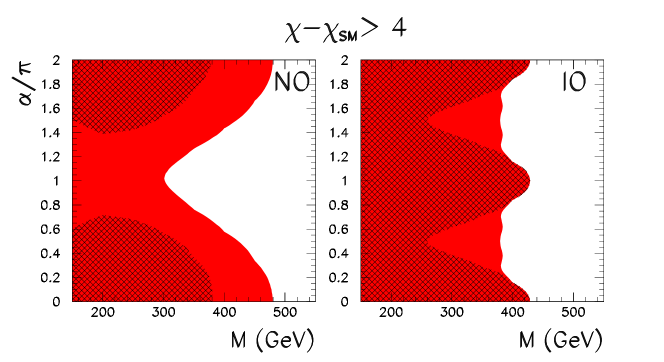
Figure 6: 95% excluded triplet mass in the MLFV Type–III see–saw scenario as a function of the unknown phase $\alpha$ from the analysis of $pp\rightarrow ll^{\prime}jj\nu\nu$ events with $l,l^{\prime}$ being either $e$ or $\mu$ of either charge observed in the LHC Run-I in ATLAS Aad:2015cxa . The full regions correspond to the likelihood function constructed including the full information given on flavour and charge of the final states (see Eq. (48)) while the hatched ones are obtained from the analysis of the total data summing over charge and flavour (see Eq. (49)). The triplet couplings have been marginalized within the ranges allowed at 95% CL by the neutrino oscillation data analysis in Ref. Esteban:2016qun for NO (left) and IO (right).

The hatched regions are the corresponding constraints obtained using only the information on the total number of events ($\chi^{2}_{tot}-\chi^{2}_{tot,SM}>4$) summed over flavour and charge of the final leptons. This figure illustrates again how using the flavour and charge information allows to impose stronger bounds on this scenario, in particular allowing to rule out triplet masses irrespective of $\alpha$ for both orderings while for NO no bound can be imposed for $70^{\circ}\pi\lesssim\alpha\lesssim 250^{\circ}$ if only the total number of events is considered.

In summary, we have shown how the analysis of the events containing two charged leptons (either electron or muons), two jets from a hadronically decaying $W$ boson in the Run I with the ATLAS detector  Aad:2015cxa can be used to impose constraints on the MLFV Type III see–saw scenario. Because of MLFV, the expected event rates in the different flavour and charge combinations of the two leptons are constrained by the existing neutrino data so the bounds cannot be evaded. For this reason it is possible to use this data to rule out these scenario with triplet masses lighter than 300 GeV at 95% CL irrespective of the neutrino mass ordering and of the value of the unknown Majorana phase parameter. The same analysis allows to rule out triplet masses masses up to 480 GeV at 95% CL for NO and $\alpha=0,\pi$. We have stressed and quantified how the information on flavour and charge information of the produced leptons is important for maximal sensitivity to MLFV.

We finish by commenting that extended sensitivity to MLFV with heavier triplets should be attainable with the data already accumulated from Run II in the same or other event topologies. For example by the analysis of the multilepton final states in CMS in Ref. CMS:2017wua which, so far, has been performed only in the context of the simplified Type–III see–saw model. Nevertheless, as previously stressed to do so it is important to make use of the flavour and charge of final state leptons which has not been made public yet. To this aim, we have made available the model files for the MLFV Type-III see-saw frwiki .

- (1) M. C. Gonzalez-Garcia and M. Maltoni, Phenomenology with Massive Neutrinos, Phys. Rept. 460 (2008) 1–129, [arXiv:0704.1800]
- (2) S. Weinberg, Baryon and Lepton Nonconserving Processes, Phys. Rev. Lett. 43 (1979) 1566–1570
- (3) P. Minkowski, at a Rate of One Out of Muon Decays?, Phys. Lett. 67B (1977) 421–428
- (4) T. Yanagida, HORIZONTAL SYMMETRY AND MASSES OF NEUTRINOS, Conf. Proc. C7902131 (1979) 95–99
- (5) M. Gell-Mann, P. Ramond, and R. Slansky, Complex Spinors and Unified Theories, Conf. Proc. C790927 (1979) 315–321, [arXiv:1306.4669]
- (6) R. N. Mohapatra and G. Senjanovic, Neutrino Mass and Spontaneous Parity Violation, Phys. Rev. Lett. 44 (1980) 912
- (7) W. Konetschny and W. Kummer, Nonconservation of Total Lepton Number with Scalar Bosons, Phys. Lett. 70B (1977) 433–435
- (8) T. P. Cheng and L.-F. Li, Neutrino Masses, Mixings and Oscillations in SU(2) x U(1) Models of Electroweak Interactions, Phys. Rev. D22 (1980) 2860
- (9) G. Lazarides, Q. Shafi, and C. Wetterich, Proton Lifetime and Fermion Masses in an SO(10) Model, Nucl. Phys. B181 (1981) 287–300
- (10) J. Schechter and J. W. F. Valle, Neutrino Masses in SU(2) x U(1) Theories, Phys. Rev. D22 (1980) 2227
- (11) R. N. Mohapatra and G. Senjanovic, Neutrino Masses and Mixings in Gauge Models with Spontaneous Parity Violation, Phys. Rev. D23 (1981) 165
- (12) R. Foot, H. Lew, X. G. He, and G. C. Joshi, Seesaw Neutrino Masses Induced by a Triplet of Leptons, Z. Phys. C44 (1989) 441
- (13) R. N. Mohapatra and J. W. F. Valle, Neutrino Mass and Baryon Number Nonconservation in Superstring Models, Phys. Rev. D34 (1986) 1642
- (14) J. Kersten and A. Yu. Smirnov, Right-Handed Neutrinos at CERN LHC and the Mechanism of Neutrino Mass Generation, Phys. Rev. D76 (2007) 073005, [arXiv:0705.3221]
- (15) M.-C. Chen and J. Huang, TeV Scale Models of Neutrino Masses and Their Phenomenology, Mod. Phys. Lett. A26 (2011) 1147–1167, [arXiv:1105.3188]
- (16) F. del Aguila and J. A. Aguilar-Saavedra, Distinguishing seesaw models at LHC with multi-lepton signals, Nucl. Phys. B813 (2009) 22–90, [arXiv:0808.2468]
- (17) J. A. Aguilar-Saavedra, P. M. Boavida, and F. R. Joaquim, Flavored searches for type-III seesaw mechanism at the LHC, Phys. Rev. D88 (2013) 113008, [arXiv:1308.3226]
- (18) CMS Collaboration, S. Chatrchyan et. al., Search for heavy lepton partners of neutrinos in proton-proton collisions in the context of the type III seesaw mechanism, Phys. Lett. B718 (2012) 348–368, [arXiv:1210.1797]
- (19) CMS Collaboration, C. Collaboration, Search for evidence of Type-III seesaw mechanism in multilepton final states in pp collisions at ,
- (20) CMS Collaboration, C. Collaboration, Search for Type-III Seesaw Heavy Fermions with Multilepton Final States using 2.3/fb of 13 TeV proton-proton Collision Data,
- (21) CMS Collaboration, C. Collaboration, Search for Heavy Lepton Partners of Neutrinos in pp Collisions at 8 TeV, in the Context of Type III Seesaw Mechanism,
- (22) ATLAS Collaboration, G. Aad et. al., Search for type-III Seesaw heavy leptons in collisions at TeV with the ATLAS Detector, Phys. Rev. D92 (2015), no. 3 032001, [arXiv:1506.0183]
- (23) ATLAS Collaboration, A. Collaboration, Search for Type III Seesaw Model Heavy Fermions in Events with Four Charged Leptons using 5.8 fb-1 of 8 TeV data with the ATLAS Detector,
- (24) C. Biggio and F. Bonnet, Implementation of the Type III Seesaw Model in FeynRules/MadGraph and Prospects for Discovery with Early LHC Data, Eur. Phys. J. C72 (2012) 1899, [arXiv:1107.3463]
- (25) R. S. Chivukula and H. Georgi, Composite Technicolor Standard Model, Phys. Lett. B188 (1987) 99–104
- (26) A. J. Buras, P. Gambino, M. Gorbahn, S. Jager, and L. Silvestrini, Universal unitarity triangle and physics beyond the standard model, Phys. Lett. B500 (2001) 161–167, [hep-ph/0007085]
- (27) G. D’Ambrosio, G. F. Giudice, G. Isidori, and A. Strumia, Minimal flavor violation: An Effective field theory approach, Nucl. Phys. B645 (2002) 155–187, [hep-ph/0207036]
- (28) V. Cirigliano, B. Grinstein, G. Isidori, and M. B. Wise, Minimal flavor violation in the lepton sector, Nucl. Phys. B728 (2005) 121–134, [hep-ph/0507001]
- (29) S. Davidson and F. Palorini, Various definitions of Minimal Flavour Violation for Leptons, Phys. Lett. B642 (2006) 72–80, [hep-ph/0607329]
- (30) M. B. Gavela, T. Hambye, D. Hernandez, and P. Hernandez, Minimal Flavour Seesaw Models, JHEP 09 (2009) 038, [arXiv:0906.1461]
- (31) R. Alonso, G. Isidori, L. Merlo, L. A. Munoz, and E. Nardi, Minimal flavour violation extensions of the seesaw, JHEP 06 (2011) 037, [arXiv:1103.5461]
- (32) P. Fileviez Perez, T. Han, G.-y. Huang, T. Li, and K. Wang, Neutrino Masses and the CERN LHC: Testing Type II Seesaw, Phys. Rev. D78 (2008) 015018, [arXiv:0805.3536]
- (33) J. Garayoa and T. Schwetz, Neutrino mass hierarchy and Majorana CP phases within the Higgs triplet model at the LHC, JHEP 03 (2008) 009, [arXiv:0712.1453]
- (34) O. J. P. Eboli, J. Gonzalez-Fraile, and M. C. Gonzalez-Garcia, Neutrino Masses at LHC: Minimal Lepton Flavour Violation in Type-III See-saw, JHEP 12 (2011) 009, [arXiv:1108.0661]
- (35) I. Esteban, M. C. Gonzalez-Garcia, M. Maltoni, I. Martinez-Soler, and T. Schwetz, Updated fit to three neutrino mixing: exploring the accelerator-reactor complementarity, JHEP 01 (2017) 087, [arXiv:1611.0151]
- (36) A. Abada, C. Biggio, F. Bonnet, M. B. Gavela, and T. Hambye, Low energy effects of neutrino masses, JHEP 12 (2007) 061, [arXiv:0707.4058]
- (37) J. Schechter and J. W. F. Valle, Comment on the Lepton Mixing Matrix, Phys. Rev. D21 (1980) 309
- (38) S. Antusch, C. Biggio, E. Fernandez-Martinez, M. B. Gavela, and J. Lopez-Pavon, Unitarity of the Leptonic Mixing Matrix, JHEP 10 (2006) 084, [hep-ph/0607020]
- (39) R. Franceschini, T. Hambye, and A. Strumia, Type-III see-saw at LHC, Phys. Rev. D78 (2008) 033002, [arXiv:0805.1613]
- (40) B. Bajc, M. Nemevsek, and G. Senjanovic, Probing seesaw at LHC, Phys. Rev. D76 (2007) 055011, [hep-ph/0703080]
- (41) F. del Aguila and J. A. Aguilar-Saavedra, Electroweak scale seesaw and heavy Dirac neutrino signals at LHC, Phys. Lett. B672 (2009) 158–165, [arXiv:0809.2096]
- (42) ATLAS Collaboration, G. Aad et. al., The ATLAS Experiment at the CERN Large Hadron Collider, JINST 3 (2008) S08003
- (43) CMS Collaboration, S. Chatrchyan et. al., The CMS experiment at the CERN LHC, JINST 3 (2008) S08004
- (44) T. Li and X.-G. He, Neutrino Masses and Heavy Triplet Leptons at the LHC: Testability of Type III Seesaw, Phys. Rev. D80 (2009) 093003, [arXiv:0907.4193]
- (45) N. D. Christensen and C. Duhr, FeynRules - Feynman rules made easy, Comput. Phys. Commun. 180 (2009) 1614–1641, [arXiv:0806.4194]
- (46) A. Alloul, N. D. Christensen, C. Degrande, C. Duhr, and B. Fuks, FeynRules 2.0 - A complete toolbox for tree-level phenomenology, Comput. Phys. Commun. 185 (2014) 2250–2300, [arXiv:1310.1921]
- (47) feynrules.irmp.ucl.ac.be/wiki
- (48) J. Alwall, R. Frederix, S. Frixione, V. Hirschi, F. Maltoni, O. Mattelaer, H. S. Shao, T. Stelzer, P. Torrielli, and M. Zaro, The automated computation of tree-level and next-to-leading order differential cross sections, and their matching to parton shower simulations, JHEP 07 (2014) 079, [arXiv:1405.0301]
- (49) T. Sjostrand, S. Mrenna, and P. Z. Skands, PYTHIA 6.4 Physics and Manual, JHEP 05 (2006) 026, [hep-ph/0603175]
- (50) DELPHES 3 Collaboration, J. de Favereau, C. Delaere, P. Demin, A. Giammanco, V. Lemaître, A. Mertens, and M. Selvaggi, DELPHES 3, A modular framework for fast simulation of a generic collider experiment, JHEP 02 (2014) 057, [arXiv:1307.6346]
- (51) M. Cacciari, G. P. Salam, and G. Soyez, FastJet User Manual, Eur. Phys. J. C72 (2012) 1896, [arXiv:1111.6097]
- (52) E. Conte, B. Fuks, and G. Serret, MadAnalysis 5, A User-Friendly Framework for Collider Phenomenology, Comput. Phys. Commun. 184 (2013) 222--256, [arXiv:1206.1599]