Simulating streamer discharges in 3D with the parallel adaptive Afivo framework

Abstract

We present an open-source plasma fluid code for 2D, cylindrical and 3D simulations of streamer discharges, based on the Afivo framework that features adaptive mesh refinement, geometric multigrid methods for Poisson’s equation, and OpenMP parallelism. We describe the numerical implementation of a fluid model of the drift-diffusion-reaction type, combined with the local field approximation. Then we demonstrate its functionality with 3D simulations of long positive streamers in nitrogen in undervolted gaps, using three examples. The first example shows how a stochastic background density affects streamer propagation and branching. The second one focuses on the interaction of a streamer with preionized regions, and the third one investigates the interaction between two streamers. The simulations run on up to $10^{8}$ grid cells within less than a day. Without mesh refinement, they would require $4\cdot 10^{12}$ grid cells.

1 Introduction

Streamer discharges [1, 2, 3] are a generic stage of electric breakdown of nonconducting matter, dominated by strong space charge effects at the tips of growing discharge channels. They occur as precursors of sparks, arcs and lightning leaders, in nature as well as in high voltage and plasma technology. Streamers are directly visible as so-called sprites in the mesosphere [4], and they are used in applications such as surface processing [5], sterilization and disinfection [6] or wound healing [7], often in the form of atmospheric pressure plasma jets [8].

Streamers grow due to strong field enhancement at the tips of their partially ionized long channels. The high local fields support the local growth of ionization due to electron impact ionization. Simulating this process has proven to be challenging for a number of reasons:

• Problems such as streamer branching or the interaction between streamers require a three-dimensional description, as illustrated in figure 1.

• A fine grid spacing is required to accurately resolve the thin charge layers around streamer heads that create the local field enhancement, see figure 2. Due to the strongly non-linear growth of streamers, it is usually not possible to obtain an approximate solution on a coarse grid.

• Time-dependent simulations are required. Due to the high electric field at streamer tips, where the mesh spacing is small, small time steps have to be used.

• At each time step, Poisson’s equation has to be solved to obtain the electrostatic potential and field. The non-local nature of this equation complicates the parallelization of streamer models.

The physics of streamer discharges is mostly governed by electrons, because ions gain energy more slowly and lose it more easily in collisions. Both plasma fluid models and kinetic/particle-in-cell models have been used to simulate streamers. In fluid models particle densities (and sometimes also momentum or energy densities) evolve in time, using pre-calculated transport coefficients as input data. In kinetic simulations, the electron distribution function $f(\vec{x},\vec{v},t)$ evolves in time, using cross sections as input data. Kinetic simulations typically require a large number of particles and smaller time steps than fluid simulations, so that their computational cost is considerably higher.

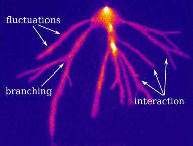
Figure 1: Experimental picture of positive streamers, showing why 3D simulations are often required: streamers branch and interact, and single streamers often show fluctuations which cannot be captured with axisymmetric models. Picture adapted from [9] (air at 293 K and 0.4 bar, 16 kV applied to a 4 cm gap).

The first demonstration of a 3D fluid simulation was given in [10]. In [11], parallel fluid simulations with adaptive mesh refinement (AMR) were performed using Paramesh, but the main bottleneck was the Poisson solver. Later work includes a 2.5D fluid model with AMR, parallelized over axial modes [12]. Kinetic [13, 14] and hybrid kinetic/fluid [15] 3D models without AMR have also been employed, and more recently kinetic models with AMR have been used [16, 17]. Other work includes 3D simulations with a finite element code [18] and a proof-of-concept of 3D simulations in transformer oil with OpenFoam [19]. A notable development was the 3D fluid model with AMR presented in [20], which is commercially available. The adaptation of parallel multigrid methods from the Gerris Flow Solver [21] made it possible to perform relatively large scale 3D simulations.

Here we present Afivo-streamer, an open-source fluid model for the simulation of streamer discharges. Both 2D, axisymmetric and 3D simulations are supported, but the focus here is on 3D, which is computationally most challenging. Afivo-streamer is based on the Afivo framework [22], which provides quadtree/octree adaptive mesh refinement, a geometric multigrid solver, shared-memory parallelism, and routines for writing output. A first successful application of Afivo-streamer can be found in [23]. The main contribution of Afivo-streamer is that it provides efficient and open-source computational infrastructure for 2D, 3D and axisymmetric streamer simulations. The paper is organized in two parts. In the first part (section 2), the numerical implementation of Afivo-streamer is described. In the second part (section 3), we demonstrate the code’s functionality with three 3D examples.

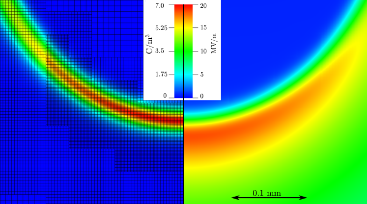
Figure 2: Cross section through a streamer head, showing the charge density (left) and electric field strength (right). The numerical mesh was generated according to the criteria described in section 2.5, using equation (8) with $c_{0}=1.0$ and $c_{1}=1.2$.

2 Model description

The implementation of the different components of Afivo-streamer is described below. The source code is available online through [24] under an open source (GPLv3) license.

2.1 Afivo AMR framework

Adaptive mesh refinement is essential for 3D streamer simulations. Without AMR, the fine grid spacing that is required near the streamer head severely restricts the size of the computational domain. Here the open-source Afivo framework [22] is used to provide AMR and parallelization for streamer simulations. The functionality of Afivo is summarized below; for more details we refer to [22].

2.1.1 Adaptive quadtree/octree grids

Afivo supports quadtree (2D) and octree (3D) grids. A quadtree/octree grid consists of blocks of $N^{D}$ cells, where $N$ is an even number (here we use $N=8$) and $D$ is the problem dimension. One or more of these blocks defines the coarse grid. A coarse grid block can be refined by covering it with $2^{D}$ child blocks, which each have half the grid spacing. This process can be repeated recursively, leading to an adaptively refined mesh that still has a quite regular structure, as illustrated in figure 3.

Afivo provides routines for adapting the mesh, but does not come with built-in refinement criteria. The criteria used here are discussed in section 2.5. Afivo does ensure proper nesting, which means that neighboring boxes differ by at most one refinement level. Methods for interpolating from coarse to fine grids, and vice versa, are included.

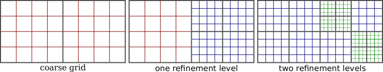
Figure 3: Left: example of a quadtree grid consisting of two blocks of $4\times 4$ cells. The middle and right figure show how the mesh can be refined by recursively adding new blocks, each having half the grid spacing of their parent.

2.1.2 Geometric multigrid solver

One of the key computational challenges in streamer simulations is quickly solving Poisson’s equation

$$\nabla\cdot(\varepsilon\nabla\phi)=-\rho,$$ (1)

to obtain the electrostatic potential $\phi$ from the charge density $\rho$, where $\varepsilon$ is the dielectric permittivity. The electrostatic field can then be determined as $\vec{E}=-\nabla\phi$. Poisson’s equation has to be solved at every time step and with high spatial resolution within the ionization fronts, and its non-local nature prevents a straightforward parallel solution. Therefore, the Poisson solver is often the most time-consuming part of streamer simulations. Afivo implements geometric multigrid routines [25, 26], which are among the fastest methods for solving elliptic equations such as (1).

Multigrid methods are iterative solvers which cycle over a hierarchy of grids. Short-wavelength errors are efficiently reduced on fine grids, and long-wavelength errors on coarse grids, by using an appropriate smoothing procedure. There are many varieties of multigrid, which differ in for example their multigrid cycle, smoothing procedure, grid hierarchy or interpolation method. For a detailed description of multigrid methods, which we cannot give here, we refer to e.g. [25, 26, 27].

Afivo supports a V-cycle and an FMG (full multigrid) cycle. An FMG cycle is more expensive than a V-cycle, but it typically gives a solution within the discretization error in one or two iterations. Both cycles are implemented using the full approximation scheme, which means that the computed solution is available at all grid levels (in some multigrid methods, only the correction to the solution is computed on coarse grids). Afivo includes Gauss-Seidel red-black smoothers that can be used for constant $\varepsilon$ problems, and to some extent also for problems where $\varepsilon$ varies, see [22]. It is currently not possible to include internal boundary conditions, for example to define a curved electrode, although work in that direction is ongoing.

For the Afivo-streamer model, an FMG cycle is used to compute the initial electric potential. For each subsequent update of the potential a number of V-cycles is used (here two), which use the previous solution as an initial guess. This exploits the fact that there are only small changes in the potential between time steps.

In streamer simulations with AMR, the fine grid ideally covers a relatively small region. As discharges propagate, the mesh has to follow their features, meaning it changes frequently in time. A key advantage of geometric multigrid methods is that they require almost no extra computation when the mesh changes, in contrast to matrix-based (direct) methods.

2.1.3 Parallelization

Afivo incorporates shared-memory parallelization using OpenMP, which means that it can use one up to e.g. 32 cores, depending on the available hardware. Since the quadtree/octree grid is naturally divided into blocks, the parallelization is performed over these blocks. Each block contains a layer of ghost cells, so that they can be operated on independently. The scaling of codes based on Afivo is typically limited by the memory bandwidth of the computer. For the multigrid methods, a further challenge is that coarse grid levels contain few data points, hampering their parallel efficiency, see e.g. [26].

2.1.4 Writing output

When doing 3D simulations with AMR, writing and visualizing output can be challenging. Afivo comes with support for writing VTK unstructured files and Silo files, which can be visualized with e.g. Visit [28]. For 3D simulations, the Silo format is more efficient, as it groups grid blocks into larger rectangular regions. The Silo files also include ghost cell information, which helps to ensure smooth visualizations near refinement boundaries. For a 3D streamer simulation, output can get pretty large: using for example 5 variables and $2\times 10^{7}$ grid cells, a single file is about a gigabyte.

2.2 Fluid model equations

The fluid model used here is of the drift-diffusion-reaction type with the local field approximation [29]. It keeps track of the electron density $n_{e}$ and the positive ion density $n_{i}$:

$$\partial_{t}n_{e} =\nabla\cdot(\mu_{e}n_{e}\vec{E}+D_{e}\nabla n_{e})+\bar{\alpha}\mu_{e}En_{e},$$ (2)

$$\partial_{t}n_{i} =\bar{\alpha}\mu_{e}En_{e}.$$ (3)

Here $\bar{\alpha}$ is the effective ionization coefficient, $\mu_{e}$ the electron mobility, $D_{e}$ the electron diffusion coefficient and $\vec{E}$ the electric field. With the local field approximation $\mu_{e}$, $D_{e}$ and $\bar{\alpha}$ are functions of the local electric field strength. These coefficients can be computed with a Boltzmann solver [30, 31] or particle swarms [32], or they can be measured experimentally. The fluid equations are coupled to the electrostatic field, which is computed as

$$\vec{E} =-\nabla\phi,$$ (4)

$$\nabla^{2}\phi =-e(n_{i}-n_{e})/\varepsilon_{0}$$ (5)

where $\phi$ is the electric potential, $\varepsilon_{0}$ the permittivity of vacuum and $e$ the elementary charge. The electric potential is computed with the multigrid routines from Afivo, described in section 2.1.

Different types of plasma fluid models can be implemented in Afivo-streamer. More advanced models could for example include an equation for the momentum and/or energy density, and let the transport coefficients depend on the mean electron energy, see e.g. [33, 34]. The mean energy is then given by $Q/n_{e}$, where $Q$ is the energy density. Such models capture more of the physics, as demonstrated in e.g. [35]. However, the ratio is $Q/n_{e}$ hard to define when $n_{e}\to 0$, making such models less robust than the one used here. Furthermore, a hyperbolic system with multiple coupled equations is generally harder to solve than a scalar one.

For electric discharges in air, photoionization is often an important process [36]. Excited nitrogen molecules can emit UV photons which are able to ionize oxygen molecules. Such a non-local source of free electrons is particularly important for positive streamers, which require free electrons ahead of them to grow. Afivo-streamer contains a Monte Carlo procedure for photoionization, which can take into account stochastic fluctuations due the finite number of photons. The procedure is described in chapter 11 of [37], and in a forthcoming paper we will investigate the effect of stochastic photoionization on streamer branching. In the present paper we focus on discharges in pure nitrogen without photoionization, using a background density of electrons and positive ions.

2.3 Spatial discretization

The spatial discretizations used in Afivo-streamer are second order accurate. We use a finite volume approach, in which the following quantities are defined at cell centers: the electron/ion density, the electric potential, and the electric field strength. The electron fluxes and the electric field components are defined at cell faces.

Afivo’s multigrid routines compute the electric potential from the charge density, as discussed in section 2.1.2. From the cell-centered electric potential $\phi$, the electric field at cell faces is computed by central differencing, so that the $x$-component is computed as

$$E_{x}^{i+1/2,j,k}=(\phi^{i,j,k}-\phi^{i+1,j,k})/\Delta x.$$

The electric field strength at cell centers is then computed as $E^{i,j,k}=\sqrt{E_{x}^{2}+E_{y}^{2}+E_{z}^{2}}$ where $E_{x}=(E_{x}^{i-1/2,j,k}+E_{x}^{i+1/2,j,k})/2$ is the average $x$-component at the cell center, $E_{y}=(E_{y}^{i,j-1/2,k}+E_{y}^{i,j+1/2,k})/2$, and similar for $E_{z}$.

We follow the approach from [38] for the discretization of the fluid equations. The advective part of the flux is computed using the Koren limiter [39]. The electron velocity at a cell face is then computed as

$$v_{x}^{i+1/2,j,k}=-\mu(E^{*})E_{x}^{i+1/2,j,k},$$

where $E^{*}=(E^{i,j,k}+E^{i+1,j,k})/2$ is the electric field strength $|\vec{E}|$ at the cell face. For brevity, we now omit the extra indices $j,k$. If $v_{x}^{i+1/2}<0$, the advective flux between cell $i$ and $i+1$ is given by

$$f_{x}^{i+1/2}=v_{x}^{i+1/2}\left(n_{e}^{i+1}-\psi\left(\frac{n_{e}^{i+2}-n_{e}^{i+1}}{n_{e}^{i+1}-n_{e}^{i}}\right)(n_{e}^{i+1}-n_{e}^{i})\right),$$ (6)

and if $v_{x}^{i+1/2}\geq 0$, it is given by

$$f_{x}^{i+1/2}=v_{x}^{i+1/2}\left(n_{e}^{i}+\psi\left(\frac{n_{e}^{i}-n_{e}^{i-1}}{n_{e}^{i+1}-n_{e}^{i}}\right)(n_{e}^{i+1}-n_{e}^{i})\right),$$ (7)

where $\psi(x)$ is the Koren limiter, given by

$$\psi(x)=\max\left(0,\min(1,(2+x)/6,x)\right).$$

The $y$ and $z$ components are computed similarly. Note that the above equations, if directly implemented, could cause division by zero. Our numerical implementation avoids this; it is described in Appendix B of [37].

The diffusive flux between cells $i$ and $i+1$ is computed using central differences, and is given by

$$f_{x}^{i+1/2}=D_{e}(E^{*})(n_{e}^{i+1}-n_{e}^{i})/\Delta x,$$

with $E^{*}$ defined as above.

To efficiently look up transport coefficients we convert them to a lookup table. This table stores the coefficients at regularly spaced electric field strengths, linearly interpolating the input data, e.g., from BOLSIG+. To look up values for a given field strength, the corresponding index in the table is computed, after which linear interpolation is employed. By default, the table is constructed up to $E_{\mathrm{max}}=35\,\textrm{MV/m}$ using 1000 entries.

Near refinement boundaries, we use linear interpolation to obtain two fine-grid ghost values, which are required for equations (6-7). These ghost cells lie inside a coarse-grid neighbor cell, and we limit them to twice the coarse value to preserve positivity. At refinement boundaries, the coarse fluxes are set to the sum of the fine fluxes to ensure mass conservation.

2.4 Temporal discretization

Time stepping is performed as in [38], using the second order accurate explicit trapezoidal rule. This method is strong stability preserving (SSP) and has favorable properties when combined with the Koren limiter [40]. Our implementation advances over $\Delta t$ as follows:

1. Store the original electron and ion densities.

2. Compute fluxes and source terms, then perform a forward Euler step over $\Delta t$ and compute a new electric field.

3. Compute fluxes and source terms, then perform another forward Euler step over $\Delta t$.

4. Average the new electron and ion densities (advanced over $2\Delta t$) with the stored initial ones. Then compute a new electric field from the resulting charge density.

All the grids are advanced using the same global time step. We limit $\Delta t$ according to several criteria. The first is a CFL condition

$$\Delta t\sum{|v_{i}|/\Delta x}<0.5$$

where $v_{i}$ are the velocity components and $\Delta x$ the grid spacing. This condition is more strict than necessary for stability, but we found that a CFL number of $0.5$ gives a good balance between accuracy and computational cost. To ensure stability for the combined advective and diffusive fluxes, we require

$$\Delta t\sum{|v_{i}|/\Delta x}+\Delta t\,(2DD_{e})/\Delta x^{2}<1.0,$$

where $D$ is the problem dimension, and $D_{e}$ the electron diffusion constant. Finally, the time step is also limited by the dielectric relaxation time

$$\Delta t<\varepsilon_{0}/(e\mu_{e}n_{e}).\\$$

These requirements for $\Delta t$ are evaluated at stage (3) of our time stepping scheme, where the required quantities are already available. The next time step is then obtained by multiplying with a safety factor (default $0.9$).

2.5 Refinement criterion

The growth of positive streamers is dominated by electron impact ionization. Therefore, our refinement criterion is based on $1/\alpha(E)$, which is the average distance between ionization events for an electron. Ignoring advection, it is an estimate for the distance over which the electron density increases by a factor of $e\approx 2.72$. For the simulations presented here, the following criterion was used

$$\Delta x<c_{0}c_{1}/\alpha(c_{1}E),$$ (8)

where we used $c_{0}=1$ and $c_{1}=1.2$. The constant $c_{1}$ was introduced to balance the refinement ahead and on the sides of the streamer. Without this constant (or when it is one), we sometimes observed oscillations in a streamer’s radius. Setting $c_{1}>1$ increases the refinement for intermediate electric fields, as illustrated in figure 4. This helps to have more refinement on the sides of streamers, without significantly increasing the refinement at their tips.

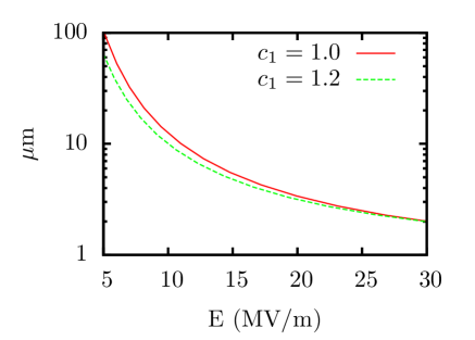
Figure 4: The refinement criterion of equation (8) for $c_{1}=1.0$ and $c_{1}=1.2$, with $c_{0}=1.0$ for both cases. With a larger value of $c_{1}$, there is more refinement at low to intermediate electric fields. Data for nitrogen at 1 bar was used for $\alpha(E)$, as described in section 3.1.

The criterion of equation (8) is evaluated for each grid cell. If at least one cell of a grid block requires refinement, the whole block is refined. Afivo implements a refinement buffer, so that blocks are also refined when nearby cells in neighboring blocks require refinement. For the simulations presented here, we used a buffer distance of three cells. Furthermore, the code places refinement around the initial conditions, to ensure they are accurately captured. Grid blocks can be derefined when for all cells equation (8) holds with $c_{0}=1/8$ and $\Delta x<\Delta x_{\mathrm{deref}}$. Here, we used $\Delta x_{\mathrm{deref}}=30\,\mu\textrm{m}$, which controls the mesh resolution of the discharge in regions where it no longer grows. An example of the resulting mesh around a streamer head is shown in figure 2. This streamer was generated in nitrogen at $1\,\mathrm{bar}$, using the same transport coefficients as for the examples presented in section 3.

The above criterion is an empirical criterion for positive streamers, which often works quite well, but not always. For example, when simulating negative streamers propagating into a zero-density region ($n_{e}=0$), the criterion will trigger refinement where there are no electrons and no space charge. We have experimented with a different criterion, based on the space charge density $\rho$: $\Delta x<\sqrt{c_{3}\varepsilon_{0}/|\rho|}$, with $c_{3}$ for example $25\,\textrm{V}$. Such a criterion captures the space charge layers quite well, but not the strong density gradients ahead of those charge layers, which play an important role in streamer propagation. In the future, we hope to find a more generic criterion, based on the discretization error in the model itself.

We would like to point out that the coarse mesh can make a significant difference in the computational cost of simulations. For example, if the finest mesh spacing required in a simulation is $2\,\mu\textrm{m}$, and the computational domain measures $(10\,\textrm{mm})^{3}$, then the actual finest mesh will have a spacing of about $1.22\,\mu\textrm{m}=10/2^{13}\,\textrm{mm}$. By using a larger or smaller computational domain, the fine-grid spacing can be made to agree better with its desired value. This would allow for larger time steps, often using a smaller total number of grid cells.

3 3D simulations

We now demonstrate the functionality of Afivo-streamer with three examples, all in 3D. The simulations were performed on a single node containing two Xeon E5-2680v4 processors ($2\times 14$ cores, at $2.4\,\textrm{GHz}$). The simulations ran for up to 24 hours, using up to $10^{8}$ grid cells. Individual output files with the 3D data were up to $5\,\textrm{gigabyte}$ in size.

3.1 Simulation conditions

The simulations presented here were performed in nitrogen at one bar. Electron transport coefficients (e.g., $\alpha$, $\mu_{e}$) were computed with Bolsig+ [30] from Phelps’ cross sections [41]. A computational domain of $(40\,\textrm{mm})^{3}$ was used, constructed from octree blocks of $8^{3}$ cells. The maximum grid spacing was set to $625\,\mu\textrm{m}$; the minimum grid spacing in the simulations was about $2.4\,\mu\textrm{m}$. A background electric field of $E_{0}=2.0\,\textrm{MV/m}$ was applied in the $-\hat{z}$ direction, which is below the ‘breakdown’ threshold for nitrogen. For a discussion of the difference between discharges in overvolted and undervolted conditions we refer to [42]. The background field is imposed by grounding the bottom boundary of the domain and applying $80\,\textrm{kV}$ at the top. On the other sides of the domain, Neumann zero boundary conditions were used for the potential. Neumann zero boundary conditions were also used for the electron density on all sides, but this had little effect on the results because the simulated streamers did not connect to boundaries.

The propagation of positive streamers requires free electrons ahead of them. In air, such electrons are often provided by photoionization. Since we here perform simulations in nitrogen, where photoionization is absent, a background density of $10^{14}\,\textrm{m}^{-3}$ electrons and positive ions is included instead. Such a density could for example be present due to previous discharges in a repetitively pulsed system [43].

To start a discharge, the background field has to be locally enhanced. We do this by placing an ionized seed of about $1.8\,\textrm{mm}$ long with a radius of about $0.15\,\textrm{mm}$. The electron and positive ion density are $10^{20}\,\textrm{m}^{-3}$ at the center, which decays at distances above $d=0.1\,\textrm{mm}$ with a so-called smoothstep profile: $1-3x^{2}+2x^{3}$, where $x=(d-0.1\,\textrm{mm})/0.1\,\textrm{mm}$. When the electrons from a seed drift upwards, the electric field at the bottom of the seed is enhanced so that a positive streamer can form.

3.2 Stochastic background density

In this example we investigate how a stochastic distribution of background ionization affects streamer propagation. A single ionized seed is placed as shown in figure 5. We then let a discharge evolve using three different background ionization distributions, for which the electron and positive ion density per cell are given by:

• Case 1: A constant value of $10^{14}\,\textrm{m}^{-3}$

• Case 2: A stochastic value $(0.5+U)\times 10^{14}\,\textrm{m}^{-3}$, where $U$ is a uniformly distributed random number between zero and one.

• Case 3: A stochastic density $2U\times 10^{14}\,\textrm{m}^{-3}$, using the same random numbers as for case 2.

The background is created at the grid level with spacing $625\,\mu\textrm{m}$ and then linearly interpolated to finer grids, so that the noise has a correlation length of $625\,\mu\textrm{m}$. Note that all three cases have the same average density of $10^{14}\,\textrm{m}^{-3}$. An example of the third case is shown in figure 5. We remark that the above distributions do not contain physically realistic fluctuations, in which case the number of electrons per cell would be Poisson-distributed.

Figure 6 shows how a positive streamer propagates for the different cases. Remarkably, the streamer velocity is nearly identical. This is consistent with previous studies [16, 44, 45], in which it was found that the streamer velocity only weakly depends on the background ionization level. The background density has a stronger effect on the morphology of the streamer. After $23\,\textrm{ns}$, case 3 shows streamer branching, while case 1 and 2 do not. The evolution of cases 2 and 3 seems closer to the experimentally observed streamers of figure 1. Our results agree with a previous study [46], in which it was found that positive streamer branching is accelerated by stochastic electron density fluctuations.

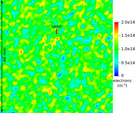
Figure 5: Cross section through the computational domain for case 3, showing a stochastic background density $2U\times 10^{14}\,\textrm{m}^{-3}$ with a correlation length of $625\,\mu\textrm{m}$, where $U$ is a uniform random number between zero and one. The location of the ionized seed from which the discharge starts is also visible, its density ($10^{20}\,\textrm{m}^{-3}$) exceeds the color scheme.

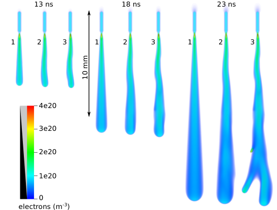
Figure 6: Evolution of a positive streamer in three background densities (1: uniform, 2: half-stochastic, 3: fully stochastic, see text). The average background density is $n_{e}=n_{i}=10^{14}\,\textrm{m}^{-3}$ for each case. Shown is a 3D volume rendering of the electron density; the opacity is indicated in the legend.

3.3 Interaction with preionization

This example is related to two previous studies [23, 47], in which the guiding of positive streamers by preionization from a laser was investigated. Here, we simulate a positive streamer passing through three preionized cylinders. The cylinders are aligned perpendicular to the direction of propagation, as indicated on the left of figure 7. They contain a density of $10^{16}$, $10^{17}$ and $10^{18}\,\textrm{m}^{-3}$ electrons and positive ions. A background density of $10^{14}\,\textrm{m}^{-3}$ was present in the whole domain.

Figure 7 shows how the electron density and electric field evolve in time. Since the fluid model employed here is deterministic, the left-right symmetry in the initial conditions is preserved. Upon reaching the first preionized region, the streamer’s maximum electric field is reduced, and it becomes slightly wider. The second patch has a similar, but somewhat stronger effect. Inside the third patch, the streamer temporarily disappears, at least when looking at the electron density. Due to the high preionization density ($10^{18}\,\textrm{m}^{-3}$) in this region, the streamer loses most of its electric field enhancement. A similar phenomenon was observed for sprite discharges, to explain the formation of so-called ‘beads’ [48]. At around $25\,\textrm{ns}$ the streamer continues, and two branches form at the boundary of the preionized cylinder. As the positive streamer grows downwards, electrons drift out towards the top. These electrons could eventually form a negative streamer, as can be seen in the electric field profiles at later times.

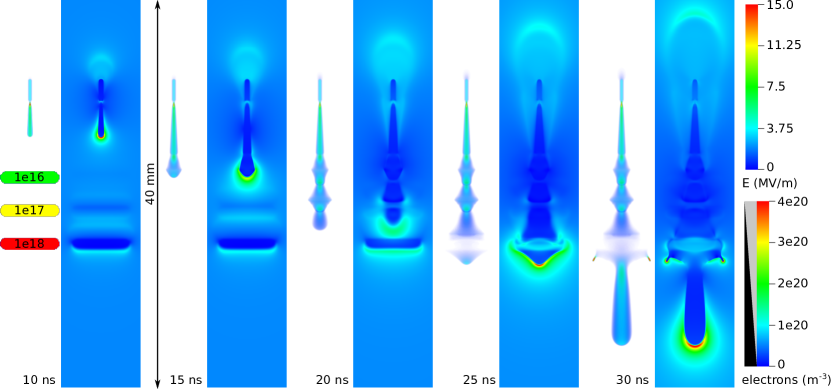
Figure 7: Evolution of a positive streamer as it propagates through preionized regions with $10^{16}$, $10^{17}$ and $10^{18}\,\textrm{m}^{-3}$ electrons and positive ions. At each indicated time a 3D volume rendering of the electron density together with a cross section of the electric field is shown.

3.4 Interacting streamers

In this example the interaction between two streamers is investigated; previous numerical and experimental investigations can be found in [12, 49]. The two interacting streamers are created by placing two field-enhancing seeds in the domain, instead of the single one used in the previous examples. We consider two cases, in which the vertical offset between the seeds is $4\,\textrm{mm}$ or $8\,\textrm{mm}$; their horizontal offset is $4\,\textrm{mm}$.

Figure 8 shows the time evolution of the electron density and the electric field for both cases, with equipotential lines indicated at steps of $4\,\textrm{kV}$. With the smaller vertical offset, the streamers repel, whereas they attract with the larger offset. This be explained by looking at the equipotential lines. For the case with the smaller vertical offset, the lower streamer bends equipotential lines downwards. This reduces the electric field in which the upper streamer propagates. The reduction is smaller farther away from the lower streamer, which causes the upper streamer to bend outwards.

For the case with the larger vertical offset, another effect becomes important. Both streamers are in total electrically neutral (as well as the seeds they originate from). Their bottom/positive end therefore bends equipotential lines downwards, whereas their upper/negative end bends them upwards. With sufficient vertical offset between the streamers, the equipotential lines between them are therefore compressed. This means there is an increased electric field between them, so that they attract. In summary, positive charged streamer heads repel, whereas a positive streamer head is attracted to a negatively charged streamer tail. Finally, notice how in both cases the bottom streamer propagates almost straight down, whereas path of the upper streamer is bent.

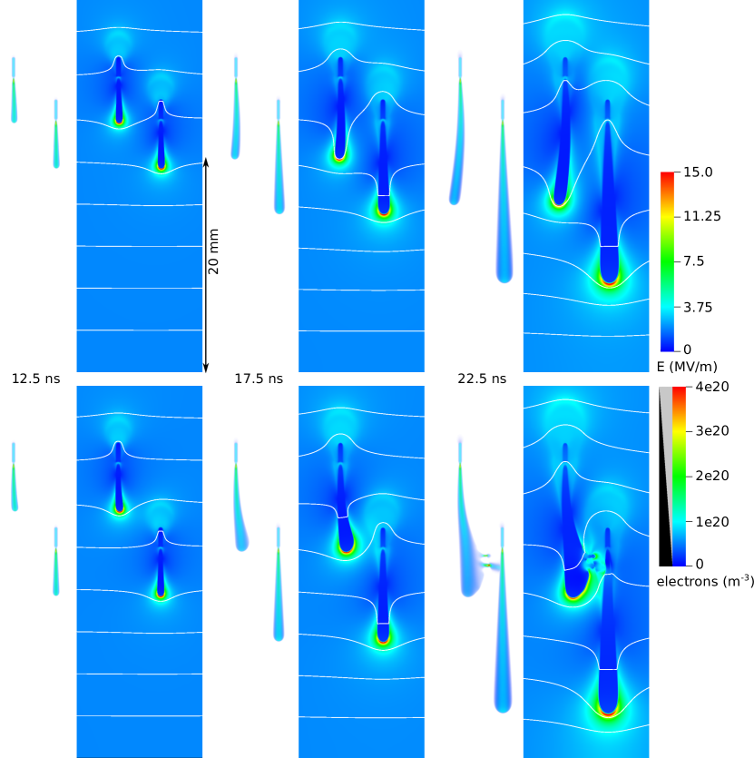
Figure 8: Evolution of two interacting positive streamers. The streamers have a vertical offset of $4\,\textrm{mm}$ (top row) or $8\,\textrm{mm}$ (bottom row) and a horizontal offset of 4 mm. At each indicated time a 3D volume rendering of the electron density together with a cross section of the electric field are shown. The white equipotential lines are spaced by $4\,\textrm{kV}$.

4 Conclusions and outlook

We have presented Afivo-streamer, an open-source plasma fluid model for 2D, cylindrical and 3D simulations of streamer discharges. The model makes use of the Afivo framework [22] to provide adaptive mesh refinement, a geometric multigrid Poisson solver and OpenMP parallelization. For robustness, the fluid model is of the drift-diffusion-reaction type in combination with the local field approximation. We have described the numerical implementation of Afivo-streamer, discussing also the refinement criterion. The model’s capabilities have been demonstrated with 3D examples of long streamers in undervolted gaps in pre-ionized nitrogen at $1\,\textrm{bar}$. The first example showed how stochastic background ionization affects streamer propagation and branching. The second demonstrated how a streamer interacts with preionized patches, in which it slows down and loses much of its field enhancement. The third example showed how streamers can attract or repel each other, depending on their relative position. These simulations used up to $10^{8}$ grid cells, and all ran within a day. A uniform grid with the same resolution would have required $4\cdot 10^{12}$ grid cells.

Future work will focus on the effects of photoionization, which was not included here, but is important for discharges in air. A numerical challenge is the inclusion of curved electrodes and dielectrics. This is planned for a future version of Afivo-streamer, and requires not only modification of the underlying Poisson solver as in [50], but also of the fluid model around the curved boundaries.

References

References

- [1] P. A. Vitello, B. M. Penetrante, and J. N. Bardsley. Simulation of negative-streamer dynamics in nitrogen. Physical Review E, 49(6):5574–5598, Jun 1994.
- [2] Won J Yi and P F Williams. Experimental study of streamers in pure N2 and N2/O2 mixtures and a cm gap. J. Phys. D: Appl. Phys., 35(3):205–218, Jan 2002.
- [3] Ute Ebert, Sander Nijdam, Chao Li, Alejandro Luque, Tanja Briels, and Eddie van Veldhuizen. Review of recent results on streamer discharges and discussion of their relevance for sprites and lightning. Journal of Geophysical Research, 115, 2010. A00E43.
- [4] D. D. Sentman and E. M. Wescott. Red sprites and blue jets: Thunderstorm-excited optical emissions in the stratosphere, mesosphere, and ionosphere. Phys. Plasmas, 2(6):2514, 1995.
- [5] M Ĉernák, D Kováĉik, J Ráhel’, P St’ahel, A Zahoranová, J Kubincová, A Tóth, and L’ Ĉernáková. Generation of a high-density highly non-equilibrium air plasma for high-speed large-area flat surface processing. Plasma Physics and Controlled Fusion, 53(12):124031, Nov 2011.
- [6] H. Akiyama. Streamer discharges in liquids and their applications. IEEE Trans. Dielect. Electr. Insul., 7(5):646–653, 2000.
- [7] Andrei Vasile Nastuta, Ionut Topala, Constantin Grigoras, Valentin Pohoata, and Gheorghe Popa. Stimulation of wound healing by helium atmospheric pressure plasma treatment. Journal of Physics D: Applied Physics, 44(10):105204, Feb 2011.
- [8] Brian L. Sands, Biswa N. Ganguly, and Kunihide Tachibana. A streamer-like atmospheric pressure plasma jet. Applied Physics Letters, 92(15):151503, Apr 2008.
- [9] T M P Briels, E M van Veldhuizen, and U Ebert. Positive streamers in air and nitrogen of varying density: experiments on similarity laws. J. Phys. D: Appl. Phys., 41(23):234008, Nov 2008.
- [10] A.A. Kulikovsky. Three-dimensional simulation of a positive streamer in air near curved anode. Physics Letters A, 245(5):445–452, Aug 1998.
- [11] S. Pancheshnyi, P. Ségur, J. Capeillère, and A. Bourdon. Numerical simulation of filamentary discharges with parallel adaptive mesh refinement. Journal of Computational Physics, 227(13):6574–6590, Jun 2008.
- [12] A. Luque, U. Ebert, and W. Hundsdorfer. Interaction of streamer discharges in air and other oxygen-nitrogen mixtures. Physical Review Letters, 101(7), Aug 2008.
- [13] O. Chanrion and T. Neubert. A PIC-MCC code for simulation of streamer propagation in air. Journal of Computational Physics, 227(15):7222–7245, Jul 2008.
- [14] D. V. Rose, D. R. Welch, R. E. Clark, C. Thoma, W. R. Zimmerman, N. Bruner, P. K. Rambo, and B. W. Atherton. Towards a fully kinetic 3D electromagnetic particle-in-cell model of streamer formation and dynamics in high-pressure electronegative gases. Phys. Plasmas, 18(9):093501, 2011.
- [15] Chao Li, Ute Ebert, and Willem Hundsdorfer. Spatially hybrid computations for streamer discharges: II. fully 3D simulations. Journal of Computational Physics, 231(3):1020–1050, Feb 2012.
- [16] Jannis Teunissen and Ute Ebert. 3d pic-mcc simulations of discharge inception around a sharp anode in nitrogen/oxygen mixtures. Plasma Sources Science and Technology, 25(4):044005, Jun 2016.
- [17] Vladimir Kolobov and Robert Arslanbekov. Electrostatic pic with adaptive cartesian mesh. Journal of Physics: Conference Series, 719:012020, May 2016.
- [18] L Papageorgiou, A C Metaxas, and G E Georghiou. Three-dimensional numerical modelling of gas discharges at atmospheric pressure incorporating photoionization phenomena. Journal of Physics D: Applied Physics, 44(4):045203, Jan 2011.
- [19] Nils Lavesson, Jonathan Jogenfors, and Ola Widlund. Modeling of streamers in transformer oil using openfoam. COMPEL - The international journal for computation and mathematics in electrical and electronic engineering, 33(4):1272–1281, Jul 2014.
- [20] V.I. Kolobov and R.R. Arslanbekov. Towards adaptive kinetic-fluid simulations of weakly ionized plasmas. Journal of Computational Physics, 231(3):839–869, Feb 2012.
- [21] Stéphane Popinet. Gerris: a tree-based adaptive solver for the incompressible euler equations in complex geometries. Journal of Computational Physics, 190(2):572–600, Sep 2003.
- [22] Jannis Teunissen and Ute Ebert. Afivo: a framework for quadtree/octree amr with shared-memory parallelization and geometric multigrid methods. Subm. to Computer Physics Communications (arXiv:1701.04329), 2017.
- [23] S Nijdam, J Teunissen, E Takahashi, and U Ebert. The role of free electrons in the guiding of positive streamers. Plasma Sources Science and Technology, 25(4):044001, May 2016.
- [24] CWI Multiscale Dynamics. Group webpage. http://cwimd.nl.
- [25] Achi Brandt and Oren E. Livne. Multigrid Techniques. Society for Industrial & Applied Mathematics (SIAM), Jan 2011.
- [26] U. Trottenberg, C.W. Oosterlee, and A. Schuller. Multigrid. Elsevier Science, 2000.
- [27] William L. Briggs, Van Emden Henson, and Steve F. McCormick. A Multigrid Tutorial (2nd Ed.). Society for Industrial & Applied Mathematics, Philadelphia, PA, USA, 2000.
- [28] Hank Childs, Eric Brugger, Brad Whitlock, Jeremy Meredith, Sean Ahern, David Pugmire, Kathleen Biagas, Mark Miller, Cyrus Harrison, Gunther H. Weber, Hari Krishnan, Thomas Fogal, Allen Sanderson, Christoph Garth, E. Wes Bethel, David Camp, Oliver Rübel, Marc Durant, Jean M. Favre, and Paul Navrátil. VisIt: An End-User Tool For Visualizing and Analyzing Very Large Data. In High Performance Visualization–Enabling Extreme-Scale Scientific Insight, pages 357–372. Chapman and Hall/CRC, Oct 2012.
- [29] A. Luque and U. Ebert. Density models for streamer discharges: Beyond cylindrical symmetry and homogeneous media. Journal of Computational Physics, 231(3):904–918, Feb 2012.
- [30] G J M Hagelaar and L C Pitchford. Solving the boltzmann equation to obtain electron transport coefficients and rate coefficients for fluid models. Plasma Sources Science and Technology, 14(4):722–733, Oct 2005.
- [31] Saša Dujko, Ute Ebert, Ronald D. White, and Zoran Lj. Petrović. Boltzmann equation analysis of electron transport in a N2-O2 streamer discharge. Japanese Journal of Applied Physics, 50(8):08JC01, Aug 2011.
- [32] Chao Li, Ute Ebert, and Willem Hundsdorfer. Spatially hybrid computations for streamer discharges with generic features of pulled fronts: I. planar fronts. Journal of Computational Physics, 229(1):200–220, Jan 2010.
- [33] Aram H Markosyan, Jannis Teunissen, Saša Dujko, and Ute Ebert. Comparing plasma fluid models of different order for 1d streamer ionization fronts. Plasma Sources Science and Technology, 24(6):065002, Oct 2015.
- [34] M M Becker, H Kählert, A Sun, M Bonitz, and D Loffhagen. Advanced fluid modeling and pic/mcc simulations of low-pressure ccrf discharges. Plasma Sources Science and Technology, 26(4):044001, Mar 2017.
- [35] O Eichwald, O Ducasse, N Merbahi, M Yousfi, and D Dubois. Effect of order fluid models on flue gas streamer dynamics. Journal of Physics D: Applied Physics, 39(1):99–107, Dec 2005.
- [36] Sergey Pancheshnyi. Photoionization produced by low-current discharges in O2, air, N2 and CO2. Plasma Sources Sci. Technol., 24(1):015023, Dec 2014.
- [37] Jannis Teunissen. 3D Simulations and Analysis of Pulsed Discharges. PhD thesis, Technische Universiteit Eindhoven, http://repository.tue.nl/801516, Nov 2015.
- [38] C. Montijn, W. Hundsdorfer, and U. Ebert. An adaptive grid refinement strategy for the simulation of negative streamers. Journal of Computational Physics, 219(2):801–835, Dec 2006.
- [39] B. Koren. A robust upwind discretization method for advection, diffusion and source terms. In C.B. Vreugdenhil and B. Koren, editors, Numerical Methods for Advection-Diffusion Problems, pages 117–138. Braunschweig/Wiesbaden: Vieweg, 1993.
- [40] W. Hundsdorfer and J. G. Verwer. Numerical Solution of Time-Dependent Advection-Diffusion-Reaction Equations. Number 33 in Springer series in computational mathematics. Springer, first edition, 2003.
- [41] A. V. Phelps and L. C. Pitchford. Anisotropic scattering of electrons by N2 and its effect on electron transport. Phys. Rev. A, 31(5):2932–2949, 1985.
- [42] Anbang Sun, Jannis Teunissen, and Ute Ebert. The inception of pulsed discharges in air: simulations in background fields above and below breakdown. J. Phys. D: Appl. Phys., 47(44):445205, Oct 2014.
- [43] S. Nijdam, E. Takahashi, A. Markosyan, and U. Ebert. Investigation of positive streamers by double pulse experiments, effects of repetition rate and gas mixture. Plasma Sources Sci. T., 23:025008, 2014.
- [44] S Nijdam, G Wormeester, E M van Veldhuizen, and U Ebert. Probing background ionization: positive streamers with varying pulse repetition rate and with a radioactive admixture. J. Phys. D: Appl. Phys., 44(45):455201, Oct 2011.
- [45] G Wormeester, S Pancheshnyi, A Luque, S Nijdam, and U Ebert. Probing photo-ionization: simulations of positive streamers in varying N2:O2-mixtures. J. Phys. D: Appl. Phys., 43(50):505201, Dec 2010.
- [46] A. Luque and U. Ebert. Electron density fluctuations accelerate the branching of positive streamer discharges in air. Phys. Rev. E, 84(4), Oct 2011.
- [47] S Nijdam, E Takahashi, J Teunissen, and U Ebert. Streamer discharges can move perpendicularly to the electric field. New Journal of Physics, 16(10):103038, Oct 2014.
- [48] A. Luque and F. J. Gordillo-Vázquez. Sprite beads originating from inhomogeneities in the mesospheric electron density. Geophysical Research Letters, 38(4), Feb 2011. L04808.
- [49] S Nijdam, C G C Geurts, E M van Veldhuizen, and U Ebert. Reconnection and merging of positive streamers in air. Journal of Physics D: Applied Physics, 42(4):045201, Jan 2009.
- [50] Sebastien Celestin, Zdenek Bonaventura, Barbar Zeghondy, Anne Bourdon, and Pierre Ségur. The use of the ghost fluid method for Poisson’s equation to simulate streamer propagation in point-to-plane and point-to-point geometries. J. Phys. D: Appl. Phys., 42(6):065203, Feb 2009.