Differentially Private Cloud-Based Multi-Agent
Optimization with Constraints

Abstract

We present an optimization framework that solves constrained multi-agent optimization problems while keeping each agent’s state differentially private. The agents in the network seek to optimize a local objective function in the presence of global constraints. Agents communicate only through a trusted cloud computer and the cloud also performs computations based on global information. The cloud computer modifies the results of such computations before they are sent to the agents in order to guarantee that the agents’ states are kept private. We show that under mild conditions each agent’s optimization problem converges in mean-square to its unique solution while each agent’s state is kept differentially private. A numerical simulation is provided to demonstrate the viability of this approach.

I Introduction

Multi-agent optimization problems arise naturally in a variety of settings including wireless sensor networks [14, 20], robotics [19], communications [13, 4], and power systems [2]. A number of approaches to solving such problems have been proposed. In [16], a distributed approach was introduced in which each agent relies only on local information in a time-varying network to solve convex optimization problems with non-differentiable objective functions. In [22] the authors present a distributed implementation of Newton’s method to solve network utility maximization problems. In [17], a distributed approach to solving consensus and set-constrained optimization problems over time-varying networks is proposed.

In the current paper, we consider inequality constrained multi-agent optimization problems and add the additional requirement that each agent’s state value be kept private. In [8] we proposed a cloud-based architecture for multi-agent optimization (without privacy) in which a cloud computer is used to handle communications and necessary global computations. We use this architecture as our starting point, though we change the cloud’s role substantially so that it keeps each agent’s state differentially private.

The notion of differential privacy was first established in the database literature as a way of providing strong practical guarantees of privacy to users contributing personal data to a database [5, 6]. Essentially differential privacy guarantees that any query of a database does not change by much if a single element of that database changes or is deleted, thereby concealing individual database entries. One appealing aspect of differential privacy is that post-processing cannot weaken its privacy guarantees, allowing for the results of differentially private queries to be freely processed [7]. In addition, differential privacy guarantees that an entry in a database cannot be determined exactly even if a malicious adversary has any arbitrary side information, e.g., other database entries [12].

Recently, differential privacy was extended to dynamical systems in [15]. Roughly, a system is differentially private if input signals which are close in the input space produce output signals which are close in the output space. This definition provides the same resilience to post-processing and protection against adversaries with arbitrary side-information mentioned above. It is this form of differential privacy which we apply here to constrained multi-agent optimization.

In the context of optimization, differential privacy has been applied in a number of ways. It was used to carry out optimization of piecewise-affine functions in [9] to keep certain terms in the objective functions private. In [11], the authors solve a distributed optimization problem in which the agents’ objective functions must be kept private. In [10], differentially private linear programs are solved while constraints or the objective function are kept private. In the current paper a saddle point finding algorithm in the vein of [8] is used to keep states private. When computations are performed using this algorithm, noises are added in accordance with the framework for differentially private dynamic systems set forth in [15] in order provide the guarantee of privacy.

The rest of the paper is organized as follows. First, Section II reviews the relevant results in the existing research literature. Then Section III formulates the specific problem to be solved here and proves that it can be solved privately. Next, Section IV provides simulation results to support the theoretical developments made. Finally, Section V concludes the paper.

II Review of Relevant Results

II-A Problem Overview

Let there be a network of $n$ agents indexed by $i\in A$, $A=\{1,\ldots,n\}$. Let each agent have a scalar state $x_{i}\in\mathbb{R}$ and let each agent have a local, convex objective function $f_{i}:\mathbb{R}\to\mathbb{R}$ that is $C^{2}$ in $x_{i}$. The function $f_{i}$ is assumed to be private in the sense that agent $i$ does not share it with other agents or the cloud. Let the agents be subject to $m$ global inequality constraints, $g_{j}:\mathbb{R}^{n}\to\mathbb{R}$, where we require

$$g_{j}(x)\leq 0$$ (1)

for all $j\in\{1,\ldots,m\}$. Here $x=(x_{1},\ldots,x_{n})^{T}\in\mathbb{R}^{n}$ contains all states in the network and we assume $g_{j}\in C^{2}$ is a convex function in $x$ for every $j$. We let $x$ takes values in a nonempty, compact, convex set $\mathcal{X}\subset\mathbb{R}^{n}$ and assume that Slater’s condition holds, namely that there is some $\bar{x}\in\mathcal{X}$ satisfying $g(\bar{x})<0$.

We can form an equivalent global optimization problem through defining a global objective function $f$ by

$$f(x)=\sum_{i=1}^{n}f_{i}(x_{i}).$$ (2)

Forming the Lagrangian of the global optimization problem, we have

$$L(x,\mu)=f(x)+\mu^{T}g(x),$$ (3)

where $\mu$ is a vector of Kuhn-Tucker (KT) multipliers in the non-negative orthant of $\mathbb{R}^{m}$, denoted $\mathbb{R}^{m}_{+}$. By definition $L(\cdot,\mu)$ is convex and $L(x,\cdot)$ is concave.

Seminal work by Kuhn and Tucker [21] showed that constrained optima of $f$ subject to $g$ are saddle points of $L$. We assume that $f$ has a unique constrained minimum and that the constrained minimum of $f$ is a regular point of $g$ so that there is a unique saddle point of $L$ [3]. The saddle point of $L$, denoted $(\hat{x},\hat{\mu})$, satisfies the inequalities

$$L(\hat{x},\mu)\leq L(\hat{x},\hat{\mu})\leq L(x,\hat{\mu})$$ (4)

for all admissible $x$ and $\mu$. One method for finding saddle points from some initial point $(x(0),\mu(0))$ is due to Bakushinskii and Polyak [1]. Letting $P_{\mathcal{X}}[\cdot]$ denote the projection onto the set $\mathcal{X}$ and $[\cdot]_{+}$ the projection onto $\mathbb{R}^{m}_{+}$, we can iteratively compute new values of $x$ and $\mu$ according to

$$x(k+1)=P_{\mathcal{X}}\bigg{[}x(k)-\gamma(k)\bigg{(}\nabla f\big{(}x(k)\big{)}+\frac{\partial g}{\partial x}\big{(}x(k)\big{)}^{T}\mu(k)+\alpha(k)x(k)\bigg{)}\bigg{]}$$ (5)

and

$$\mu(k+1)=\bigg{[}\mu(k)+\gamma(k)\big{(}g\big{(}x(k)\big{)}-\alpha(k)\mu(k)\big{)}\bigg{]}_{+}.$$ (6)

Above, $k$ is the iteration number, and $\alpha(k)$ and $\gamma(k)$ are defined as

$$\gamma(k)=\bar{\gamma}k^{-c_{1}}\textnormal{ and }\alpha(k)=\bar{\alpha}k^{-c_{2}}.$$ (7)

The constants $\bar{\gamma}$, $\bar{\alpha}$, $c_{1}$, and $c_{2}$ are selected by the user, with $c_{1}$ and $c_{2}$ subject to the conditions

$$0<c_{2}<c_{1}\textnormal{ and }c_{1}+c_{2}<1.$$ (8)

One appealing aspect of the above method in this setting is its robustness to noise in the values of $g$ and $\frac{\partial g}{\partial x}$. Define $G(x(k))=g(x(k))+w_{g}(k)$ and $\partial_{x}G(x(k))=\frac{\partial g}{\partial x}\big{(}x(k)\big{)}+w_{\partial g}(k)$, where $w_{g}(k)$ and $w_{\partial g}(k)$ are i.i.d. noises of the appropriate dimension. Then the noisy forms of Equations (5) and (6) are

$$x(k+1)=P_{\mathcal{X}}\bigg{[}x(k)-\gamma(k)\big{(}\nabla f\big{(}x(k)\big{)}+\partial_{x}G(x(k))^{T}\mu(k)+\alpha(k)x(k)\big{)}\bigg{]}$$ (9)

and

$$\mu(k+1)=\big{[}\mu(k)+\gamma(k)\big{(}G(x(k))-\alpha(k)\mu(k)\big{)}\big{]}_{+}.$$ (10)

It is this noisy form of update rule that will be used in the remainder of the paper. We use it to define Algorithm 1, below.

Algorithm 1
Step 0: Select a starting point $\big{(}x(0),\mu(0)\big{)}\in\mathcal{X}\times\mathbb{R}^{m}$ and constants, $\bar{\alpha}$, $\bar{\gamma}$, $c_{1}$, and $c_{2}$. Set $k=0$.
Step 1: Compute

$$x(k+1)=P_{\mathcal{X}}\big{[}x(k)-\gamma(k)\big{(}\nabla f\big{(}x(k)\big{)}+\partial_{x}G(x(k))^{T}\mu(k)+\alpha(k)x(k)\big{)}\big{]},$$ (11)

$$\mu(k+1)=\big{[}\mu(k)+\gamma(k)\big{(}G(x(k))-\alpha(k)\mu(k)\big{)}\big{]}_{+}.$$ (12)

Step 2: Set $k=k+1$ and return to Step 1. $\triangle$

For the purpose of analyzing the convergence of Algorithm 1, we have the following definition.

Definition 1

Let $(\hat{x},\hat{\mu})$ denote the unique saddle point of the Lagrangian as defined in Equation (3). We say Algorithm 1 converges if it generates a sequence $\big{(}x(k),\mu(k)\big{)}$ that converges in mean-square to $(\hat{x},\hat{\mu})$ in the Euclidean norm, i.e., if

$$\lim_{k\to\infty}\mathbb{E}\big{(}\|x(k)-\hat{x}\|_{2}^{2}\big{)}=0$$ (13)

and

$$\lim_{k\to\infty}\mathbb{E}\big{(}\|\mu(k)-\hat{\mu}\|_{2}^{2}\big{)}=0.$$ (14)

$\triangle$

We now present the following theorem concerning the convergence of Algorithm 1.

Theorem 1

Algorithm 1 converges in the sense of Definition 1 if the following four conditions are met:

1. $f_{i}$ and $g_{j}$ are convex and $C^{1}$ for all $i$ and $j$

2. $\mathcal{X}$ is a convex, closed, bounded set

3. Slater’s condition holds, i.e., there is some $\bar{x}\in\mathcal{X}$ such that $g(\bar{x})<0$

4. all noises are zero mean, have bounded variance, and are independent at different points

Proof: See [18]. $\blacksquare$

By assumption, Conditions 1, 2, and 3 hold. It remains to be shown that Condition 4 can hold when differential privacy is desired. This will be shown in Section III. Below we describe an implementation of Algorithm 1 and then cover differential privacy.

II-B Cloud Architecture

Let the conditions and assumptions of Section II-A hold. In [8], a cloud-based architecture was used and it was assumed that there was no inter-agent communication. This assumption is kept in force throughout this paper to enable privacy of agents’ states. In this architecture, each agent stores and manipulates its own state $x_{i}(k)\in\mathbb{R}$. Similarly, the cloud stores and updates $\mu^{c}(k)$, a vector of KT multipliers, as well as $x^{c}(k)$, the vector of each agent’s state; it does not share $x^{c}(k)$ with the agents but instead only uses it to compute values of $\mu^{c}$.

At each timestep $k$, the agents receive information from the cloud, update their states, and then send their updated states to the cloud. At the same time that the agents are updating their states, the cloud is computing an update to $\mu^{c}$ which will be sent to the agents in the next transmission the cloud sends. As mentioned above, the agents do not talk to each other at all. The role of the cloud is to serve as a trusted central aggregator for information so that computations based upon sensitive, global information, namely $\frac{\partial g}{\partial x^{c}_{i}}$ and updates to $\mu^{c}$, can be computed and the results disseminated to the agents without any agent ever directly knowing another agent’s state.

Before any optimization takes place, let agent $i$ be initialized with $f_{i}$, $\bar{\alpha}$, $\bar{\gamma}$, $\mathcal{X}$, $c_{1}$, $c_{2}$, and some initial state, $x_{i}(0)$. Let the cloud be initialized with $g$, $\frac{\partial g}{\partial x^{c}_{i}}$ for every $i$, $\bar{\alpha}$, $\bar{\gamma}$, $c_{1}$, $c_{2}$, and some initial KT vector, $\mu^{c}(0)$, that is not based on the values of any initial states. To initialize the system, each agent sends its state to the cloud. Then at each timestep, $k$, three actions occur. First, agent $i$ receives a transmission containing private versions $\frac{\partial g}{\partial x^{c}_{i}}\big{(}x^{c}(k)\big{)}$ and $\mu^{c}(k)$ from the cloud (the details of the privacy will be explained in Section III). Second, agent $i$ computes $x_{i}(k+1)$, and simultaneously the cloud computes $\mu^{c}(k+1)$. Third, agent $i$ sends $x_{i}(k+1)$ to the cloud, and then this cycle of communication and computation is repeated with the newly computed values.

Writing out the update equations for a multi-agent implementation of Algorithm 1 using the cloud architecture, we see that agent $i$ updates according to

$$x_{i}(k+1)=P_{\mathcal{X}}\Bigg{[}x_{i}(k)-\gamma(k)\bigg{(}\frac{df_{i}}{dx_{i}}\big{(}x_{i}(k)\big{)}+\partial_{x_{i}}G(x^{c}(k))^{T}\mu^{c}(k)+\alpha(k)x_{i}(k)\bigg{)}\Bigg{]}$$ (15)

and the cloud updates according to

$$\mu^{c}(k+1)=\bigg{[}\mu^{c}(k)+\gamma(k)\big{(}G(x^{c}(k))-\alpha(k)\mu^{c}(k)\big{)}\bigg{]}_{+},$$ (16)

where $\partial_{x_{i}}G(x^{c}(k))=\frac{\partial g}{\partial x^{c}_{i}}\big{(}x^{c}(k)\big{)}+w_{i}(k)$ and, as before, $G\big{(}x^{c}(k)\big{)}=g(x^{c}(k))+w_{g}(k)$. The distributions of all noises $w_{i}$ and $w_{g}$ will be defined in Section III. In Equation (15), the notation $\mu^{c}(k)$ is meant to indicate that at time $k$, agent $i$ updates its state using the KT vector it just received from the cloud computer; before the cloud computes a new value of $\mu^{c}$, this KT vector is equal to the $\mu$ vector stored on the cloud at time $k$, $\mu^{c}(k)$, and hence is denoted as such.

Due to the structure of communications in the system, agent $i$ receives $\partial_{x_{i}}G(x(k))$ and $\mu^{c}(k)$ before computing $x_{i}(k+1)$. Similarly, the cloud receives the agents’ states at time $k$ (which end up being the contents of the vector $x^{c}(k)$) before computing $\mu^{c}(k+1)$. Then despite the distributed nature of the problem, all information in the network is synchronized whenever updates are computed anywhere. This means that, in aggregate, the steps taken by the agents and cloud using Equations (15) and (16) are identical to those used in Algorithm 1 to solve the global optimization problem defined in Section II-A. As a result, the analysis for the convergence of the cloud-based implementation of Algorithm 1 will be carried out using the centralized form of Algorithm 1 as presented in Section II-A, and it will apply to the cloud-based problem.

II-C Differential Privacy for Dynamic Systems

Let there be $n$ input signals to a system, each contributed by some user. Let the $i^{th}$ input signal be denoted $u_{i}\in\ell^{s_{i}}_{p_{i}}$. Here $s_{i}\in\mathbb{N}$ is the dimension of the signal and, with an abuse of notation, we say $u_{i}\in\ell^{s_{i}}_{p_{i}}$ if each finite truncation of $u_{i}$ has finite $p_{i}$-norm, i.e., if

$$u_{0:k}:=(u(0)^{T},u(1)^{T},\ldots,u(k)^{T})^{T}$$ (17)

has finite $p_{i}$-norm for all $k$.

Using this definition, the full input space to the system is

$$\ell_{p}^{s}=\ell^{s_{1}}_{p_{1}}\times\ell^{s_{2}}_{p_{2}}\times\cdots\times\ell^{s_{n}}_{p_{n}},$$ (18)

and the system generates outputs $y\in\ell^{r}_{q}$ with $q,r\in\mathbb{N}$. Fix a set of non-negative real numbers $b=(b_{1},\ldots,b_{n})$. We define a symmetric binary adjacency relation, $\textnormal{Adj}(\cdot,\cdot)$, on the space $\ell^{s}_{p}$ such that

$$\textnormal{Adj}_{b}(u,\tilde{u})=1\textnormal{ if and only if }\|u_{i}-\tilde{u}_{i}\|_{p_{i}}\leq b_{i}\textnormal{, }\textnormal{for some $i$ and }u_{j}=\tilde{u}_{j}\textnormal{ for all }j\neq i.$$ (19)

In words, $\textnormal{Adj}(u,\tilde{u})$ holds if and only if $u$ and $\tilde{u}$ differ by (at most) one component and this difference is bounded by the corresponding element of $b$. In this paper, we will focus exclusively on the case that ${p_{i}=2}$ for every $i$. The symbol $\|\cdot\|_{2}$ will be used for both the Euclidean norm and the $\ell_{2}$ norm, though the meaning of each use is clear from context.

Roughly, differential privacy guarantees that if two input signals are adjacent, their output signals should not differ by too much. As a result, small changes to inputs are not seen at the output and someone, e.g., a malicious eavesdropper, with access to the output of the of the system cannot exactly determine the input. To make this notion precise, let us fix a probability space $(\Omega,\mathcal{F},\mathbb{P})$. Let $\mathcal{R}^{d}$ denote the Borel $\sigma$-algebra defined on $\mathbb{R}^{d}$. In the setting of differentially private dynamic systems, a mechanism is a stochastic process $M$ of the form

$$M:\ell^{s}_{p}\times\Omega\to\ell^{r}_{q},$$ (20)

i.e., $M$ has inputs in $\ell^{s}_{p}$ and sample paths in $\ell^{r}_{q}$. We now state a lemma concerning differentially private mechanisms for dynamical systems.

Lemma 1

A mechanism $M:\ell^{s}_{p}\times\Omega\to\ell^{r}_{q}$ is $(\epsilon,\delta)$-differentially private if and only if for every $u,\tilde{u}\in\ell^{s}_{p}$ satisfying $\textnormal{Adj}_{b}(u,\tilde{u})$, we have

$$\mathbb{P}\big{(}(Mu)_{0:k}\in S\big{)}\leq e^{\epsilon}\mathbb{P}\big{(}(M\tilde{u})_{0:k}\in S)+\delta,\forall k\geq 0,\forall S\in\mathcal{R}^{(k+1)r}.$$ (21)

Proof: See [15], Lemma 2. $\blacksquare$

Equation (21) captures in a precise way the notion that, at each time $k$, truncated outputs up until $k$ that correspond to adjacent inputs must have similar probability distributions, with the level of similarity of the outputs determined by $\delta$ and $\epsilon$. Indeed, the constants $\epsilon$ and $\delta$ determine the level of privacy afforded by the mechanism $M$ to users contributing input signals. Generally, $\epsilon$ is kept small, e.g., $0.1$, $\ln 2$, or $\ln 3$. The parameter $\delta$ should be kept very small because it allows a zero probability event for $\tilde{u}$ to be a non-zero probability event for $u$ and thus controls when there can noticeable differences in outputs which correspond to adjacent inputs. The choice of $b$ determines which inputs to the system should produce similar outputs and thus determines which inputs should “look alike” at the output.

One appealing aspect of differential privacy is that its privacy guarantees cannot be weakened by post-processing. Given the output of a differentially private mechanism, that output can be processed freely without threatening the privacy of the inputs. In addition, this privacy guarantee holds even against an adversary with arbitrary side information. Even if an adversary gains knowledge of, e.g., some number of inputs, that adversary still cannot determine exactly the system’s other input signals by observing its outputs. In the present paper, Equation (21) will be used as the definition of differential privacy and the reader is referred to [15] for a proof of Lemma 1.

Before discussing the mechanisms to be used here, we first define the $\ell_{2}$ sensitivity of a system; while the $\ell_{p}$ sensitivity can be used for other values of $p$, we focus on $p=2$ in this paper. Let $\mathcal{G}$ be a deterministic causal system. The $\ell_{2}$ sensitivity is an upper bound, $\Delta_{2}$, on the norm of the difference between the outputs of $\mathcal{G}$ which correspond to adjacent inputs. That is, $\Delta_{2}$ must satisfy

$$\|\mathcal{G}u-\mathcal{G}\tilde{u}\|_{2}\leq\Delta_{2}$$ (22)

whenever $\textnormal{Adj}_{b}(u,\tilde{u})$ holds. There are several established differentially private mechanisms in the literature, e.g., [7, Chapter 3], though here we will use only the Gaussian mechanism in the lemma below. In it, we use the $\mathcal{Q}$-function, defined as

$$\mathcal{Q}(x)=\frac{1}{\sqrt{2\pi}}\int_{x}^{\infty}e^{-\frac{u^{2}}{2}}du.$$ (23)

Lemma 2

The mechanism $Mu=\mathcal{G}u+w$ is $(\epsilon,\delta)$-differentially private if $w\sim\mathcal{N}(0,\sigma^{2}I_{r})$, where $I_{r}$ is the identity matrix of the same dimension as the output space, $\ell_{q}^{r}$, and where $\sigma$ satisfies

$$\sigma\geq\Delta_{2}\kappa(\delta,\epsilon)$$ (24)

where we define $K_{\delta}=\mathcal{Q}^{-1}(\delta)$ and

$$\kappa(\delta,\epsilon):=\frac{1}{2\epsilon}\left(K_{\delta}+\sqrt{K_{\delta}^{2}+2\epsilon}\right).$$ (25)

Proof: See [15]. $\blacksquare$

We will use $\kappa(\delta,\epsilon)$ in Equation (25) for the remainder of the paper. Lemma $2$ says in a rigorous way that adding noise to the true output of a system can make it differentially private, provided the distribution from which the noise is drawn has large enough variance. Also from Lemma 2, we see that once $\epsilon$ and $\delta$ are chosen, we need only to find the $\ell_{2}$ sensitivity of a system, $\Delta_{2}$, to calibrate the level of noise that must be added to guarantee differential privacy. We do this in the next section for the optimization problem outlined above.

III Private Optimization

Based on the optimization algorithm devised in Section II and the cloud-based architecture, it is clear that two pieces of information must be shared with agent $i$ at each time $k$: $\frac{\partial g}{\partial x^{c}_{i}}\big{(}x(k)\big{)}$ and $\mu^{c}(k)$. In order to keep the agents’ states private from each other, we must then alter these quantities, or the way in which they are computed, before they are sent to the agents.

We regard each $\frac{\partial g}{\partial x^{c}_{i}}$ as a dynamic system with output $y_{i}(k)\in\ell_{2}^{m}$ at time $k$, where $m$ is the number of constraints as defined in Section II-A. Noise is added to each $y_{i}$ before it is sent to the agents in order to guarantee differential privacy of each agent’s state. While agent $i$ will only make use of $\frac{\partial g}{\partial x^{c}_{i}}$ in its computations, we assume that each agent has access to each output, i.e. agent $i$ has knowledge of $\frac{\partial g}{\partial x^{c}_{j}}$ at each time even if $j\neq i$.

To ensure that no state values can be determined from $\mu^{c}$, we use the resilience of differential privacy to post-processing. Specifically, rather than adding noise to $\mu^{c}$ directly each time it is sent to the agents, we regard $g$ as a dynamic system and add noise to the value of $g$ when computing $\mu^{c}$ in the cloud to guarantee that $g$ keeps $x^{c}$ differentially private. In doing this, $\mu^{c}$ then also keeps $x^{c}$ differentially private. In regarding $g$ as a dynamical system and setting $y_{g}(k)=g(x^{c}(k))$, we see that its output $y_{g}\in\ell_{2}^{m}$, where $m$ is the number of constraints as defined above. In this framework, $\mu^{c}$ and each $\frac{\partial g}{\partial x^{c}_{i}}$ conceal each other agent’s state from agent $i$ and any eavesdropper intercepting the cloud’s transmissions to the agents.

To define differentially private mechanisms for $\frac{\partial g}{\partial x^{c}_{i}}$, we first find bounds on the $\ell_{2}$ sensitivity of $\frac{\partial g}{\partial x^{c}_{i}}$. By assumption, $g\in C^{2}$ so that $\frac{\partial^{2}g}{\partial x_{i}^{c,2}}$ is continuous. Also by assumption, $\mathcal{X}$ is compact so that $\left\|\frac{\partial^{2}g}{\partial x_{i}^{c,2}}(x)\right\|_{2}$ attains its maximum on $\mathcal{X}$. Denote this maximum by $K^{i}_{g^{\prime}}$. We see that $K^{i}_{g^{\prime}}$ is the Lipschitz constant for $\frac{\partial g}{\partial x^{c}_{i}}$. Regarding $\frac{\partial g}{\partial x^{c}_{i}}$ as a system with inputs in $\mathbb{R}^{n}$ and outputs in $\mathbb{R}^{m}$, we have the following theorem concerning a differentially private mechanism whose output will be released to the agents.

Theorem 2

Let $K_{g^{\prime}}^{i}$ be the Lipschitz constant of $\frac{\partial g}{\partial x^{c}_{i}}$ over the domain $\mathcal{X}$ and define $B=\max_{i\in A}\{b_{i}\}$. Then the mechanism

$$M_{g^{\prime}}^{i}x^{c}(k)=\frac{\partial g}{\partial x^{c}_{i}}\big{(}x(k)\big{)}+w_{i}(k)$$ (26)

is differentially private with $w_{i}(k)\sim\mathcal{N}(0,\sigma_{i}^{2}I_{m})$, where $m$ is the number of constraints, and with $\sigma_{i}$ satisfying

$$\sigma_{i}\geq\kappa(\delta,\epsilon)K_{g^{\prime}}^{i}B.$$ (27)

Proof: For two signals, $x$ and $\tilde{x}$ in $\ell_{p}^{s}$, satisfying $\textnormal{Adj}_{b}(x,\tilde{x})$ for $b=(b_{1},\ldots,b_{n})$, we have

$$\left\|\frac{\partial g}{\partial x_{i}^{c}}(x(k))-\frac{\partial g}{\partial x_{i}^{c}}(\tilde{x}(k))\right\|_{2}\leq K^{i}_{g^{\prime}}\|x(k)-\tilde{x}(k)\|_{2}\leq K^{i}_{g^{\prime}}\|x-\tilde{x}\|_{2}\leq K^{i}_{g^{\prime}}b_{i}\leq K^{i}_{g^{\prime}}B.$$ (28)

Using this bound on the $\ell_{2}$ sensitivity of $\frac{\partial g}{\partial x^{c}_{i}}$, for each $i\in A$ we define $\sigma_{i}$ by

$$\sigma_{i}\geq\kappa(\delta,\epsilon)K^{i}_{g^{\prime}}B,$$ (29)

with $\kappa(\delta,\epsilon)$ defined as before. The theorem is then a straightforward application of Lemma 2. $\blacksquare$

To keep the agents’ states private in releasing $\mu$ we rely on the resilience to post-processing of differential privacy and compute $\mu$ using a differentially private form of $g$. As above, we note that $\frac{\partial g}{\partial x}$ itself is continuous by assumption and that there exists some $K_{g}$ satisfying

$$\left\|\frac{\partial g}{\partial x}(x)\right\|_{2}\leq K_{g}$$ (30)

for all $x\in\mathcal{X}$. By definition, $K_{g}$ is the Lipschitz constant of $g$ and we use this to define a mechanism for making $g$ private in the next theorem below. We omit the proof of this theorem due to its similarity to the proof of Theorem 2 above.

Theorem 3

Let $K_{g}$ be the Lipschitz constant of $g$ over $\mathcal{X}$ and define $B=\max_{i\in A}\{b_{i}\}$. Then the mechanism

$$M_{g}x^{c}(k)=g\big{(}x^{c}(k)\big{)}+w_{g}(k)$$ (31)

is differentially private with $w_{g}(k)\sim\mathcal{N}(0,\sigma_{g}^{2}I_{m})$, where $m$ is the number of constraints, and with $\sigma_{g}$ satisfying

$$\sigma_{g}\geq\kappa(\delta,\epsilon)K_{g}B.$$ (32)

$\blacksquare$

Under the assumptions already made in crafting the optimization problem in Section II, conditions $1-3$ of Theorem 1 are satisfied. To satisfy condition $4$ of Theorem 1, we need only to select values of $\sigma_{i}$ and $\sigma_{g}$ that are bounded above. Then Algorithm 1 will converge. In addition, as long as $\sigma_{i}$ and $\sigma_{g}$ are bounded below as in Equations (29) and (32), respectively, the conditions for $(\epsilon,\delta)$-differential privacy are simultaneously met. Importantly, Algorithm 1 is robust to noise appearing in exactly the places it is injected for privacy. Adding more noise will increase the time required for Algorithm 1 to converge and thus there is a natural trade-off: increased privacy results in a slower convergence rate because more noise is added, while decreased privacy allows for faster convergence because it reduces the noise added.

IV Simulation Results

A numerical simulation was conducted to support the theoretical developments of this paper. The problem here involves $n=7$ agents and $m=4$ constraints. The set $\mathcal{X}=[-10,10]^{7}$. This set can represent, e.g., the area a team of robots must stay inside in order to maintain communication links. The constraint function $g$ was chosen to be

$$g(x)=\left(\begin{array}[]{c}x_{1}+x_{2}+x_{3}-3\\ x_{5}^{2}+\frac{1}{12}x_{6}^{4}+\frac{1}{12}x_{7}^{4}-20\\ x_{3}^{2}+x_{4}+x_{6}-1\\ x_{6}^{2}+x_{7}^{2}-5\end{array}\right).$$ (33)

Over $\mathcal{X}$, the Lipschitz constant of $g$ was found to be approximately $K_{g}=472.567$. Each dynamic system $\frac{\partial g}{\partial x^{c}_{i}}$ and its Lipschitz constant over the domain $\mathcal{X}$ is listed in Table I.

$i$	$\frac{\partial g}{\partial x^{c}_{i}}$	$K_{g^{\prime}}^{i}$
$1$	$(1,0,0,0)^{T}$	$0$
$2$	$(1,0,0,0)^{T}$	$0$
$3$	$(1,0,2x_{3},0)^{T}$	$2$
$4$	$(0,0,1,0)^{T}$	$0$
$5$	$(0,2x_{5},0,0)^{T}$	$2$
$6$	$(0,\frac{1}{3}x_{6}^{3},1,2x_{6})^{T}$	$100.08$
$7$	$(0,\frac{1}{3}x_{7}^{3},0,2x_{7})^{T}$	$100.08$

TABLE I: Derivatives of $g$ and their Lipschitz constants

Although the Lipschitz constants in Table I are quite different, it was desired to have the level of privacy guaranteed by each mechanism be identical. The values $\delta=0.05$ and $\epsilon=\ln 3$ were chosen to be used by all systems, giving ${\kappa(\delta,\epsilon)=1.7565}$. In addition, it was desired to make agent $i$’s state difficult to distinguish from a ball of radius $1$ around it in the space $\ell^{1}_{2}$, leading to the choice of $b_{i}=1$ for all $i$, giving

$$b=(1,1,1,1,1,1,1)^{T}.$$ (34)

Using these values, the distributions of noises to be added to each $\frac{\partial g}{\partial x^{c}_{i}}$ were determined and are shown in Table II.

Noise	Distribution
$w_{1}$	$\mathcal{N}(0,0)$
$w_{2}$	$\mathcal{N}(0,0)$
$w_{3}$	$\mathcal{N}(0,12.3406I_{4})$
$w_{4}$	$\mathcal{N}(0,0)$
$w_{5}$	$\mathcal{N}(0,12.3406I_{4})$
$w_{6}$	$\mathcal{N}(0,30900.7580I_{4})$
$w_{7}$	$\mathcal{N}(0,30900.7580I_{4})$

TABLE II: Distributions of noise added to each $\frac{\partial g}{\partial x^{c}_{i}}$

In addition, the noise added to $g$ when computing $\mu$ was

$$w_{g}\sim\mathcal{N}(0,688971.6017I_{4}),$$ (35)

and the sum of the agents’ objective functions was

$$f(x)=(x_{1}-9)^{2}+x_{1}+(x_{2}+4)^{4}+(x_{3}-1)^{8}+x_{4}^{2}+(x_{4}+6)+(x_{5}+3)^{6}+(x_{6}-7)^{2}+(x_{7}-5)^{2}.$$ (36)

For Algorithm 1, the values $\bar{\gamma}=0.0005$, $\bar{\alpha}=0.20$, $c_{1}=\frac{1}{3}$ and $c_{2}=\frac{1}{4}$ were chosen. Having selected everything needed, a simulation was run that consisted of $500,000$ timesteps. The primal and dual components of the saddle point of $L$ were computed ahead of time to be approximately

$$\hat{x}=\left(7.591,-4.769,0.178,-0.822,-2.863,1.790,1.340\right)^{T}$$ (37)

and

$$\hat{\mu}=(1.8139,0,0.6409,2.7314)^{T}.$$ (38)

To illustrate the convergence of the algorithm, the values of $\|x(k)-\hat{x}\|_{2}$ and $\|\mu(k)-\hat{\mu}\|_{2}$ for $k=1,\ldots,500,000$ are plotted in Figure 1. We see that the distance from $x(k)$ to $\hat{x}$ decreases almost monotonically in early iterations and oscillates more later on, though there is a discernible decreasing trend while it oscillates. Similarly, we see that the distance from $\mu(k)$ to $\hat{\mu}$ also follows a generally decreasing trend over time. The error values after $200,000$ iterations were $\|x(200,000)-\hat{x}\|_{2}=0.4839$ and ${\|\mu(200,000)-\hat{\mu}\|_{2}=0.5459}$, indicating close convergence to the unique saddle point after the first $200,000$ iterations. Numerically, these distances to the optimum are generally within the acceptable tolerance of error for many applications. For applications with tighter bounds on the required distance to the optimum, the algorithm can simply be run for longer. In this case, after $500,000$ iterations the error values were $\|x(500,000)-\hat{x}\|_{2}=0.2612$ and ${\|\mu(500,000)-\hat{\mu}\|_{2}=0.2123}$, indicating noticeable decreases in the level of sub-optimality in $x(k)$ and $\mu(k)$.

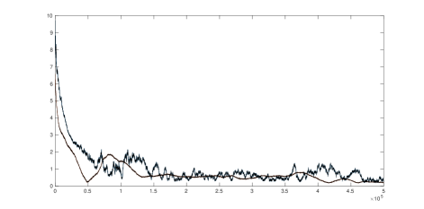
Figure 1: Values of $\|x(k)-\hat{x}\|$ (jagged line) and $\|\mu(k)-\hat{\mu}\|$ (smooth line) for $k=1,\ldots,500,000$.

The relative value of reducing oscillations and increasing privacy will vary between problems and should be considered when designing problems and selecting $\epsilon$, $\delta$, and $b$. Regardless of the weight of these two objectives, differentially private multi-agent optimization successfully converges when agents do not directly share their states, and indeed converges when it is impossible for any agent to discover exactly any other agent’s state value.

V Conclusion

A multi-agent optimization problem was considered in which it is desirable to keep each agent’s state private. This was achieved via a primal-dual optimization method and by using differential privacy. It was shown that the conditions required for differential privacy and for convergence of the optimization algorithm can be simultaneously satisfied and thus that differentially private multi-agent optimization with constraints is possible. Numerical results were then provided to attest to the viability of this approach.

References

- [1] AB Bakushinskii and BT Polyak. Solution of variational inequalities. Doklady Akademii Nauk SSSR, 219(5):1038–1041, 1974.
- [2] S. Caron and G. Kesidis. Incentive-based energy consumption scheduling algorithms for the smart grid. In Smart Grid Communications (SmartGridComm), 2010 First IEEE International Conference on, pages 391–396, Oct 2010.
- [3] Benoit Chachuat. Nonlinear and dynamic optimization: From theory to practice. Technical report, Automatic Control Laboratory, EPFL, Switzerland, 2007.
- [4] Mung Chiang, S.H. Low, A.R. Calderbank, and J.C. Doyle. Layering as optimization decomposition: A mathematical theory of network architectures. Proceedings of the IEEE, 95(1):255–312, Jan 2007.
- [5] Cynthia Dwork. Differential privacy. In 33rd International Colloquium on Automata, Languages and Programming, part II (ICALP 2006), volume 4052 of Lecture Notes in Computer Science, pages 1–12, Venice, Italy, July 2006. Springer Verlag.
- [6] Cynthia Dwork, Krishnaram Kenthapadi, Frank McSherry, Ilya Mironov, and Moni Naor. Our data, ourselves: Privacy via distributed noise generation. In Advances in Cryptology (EUROCRYPT 2006), volume 4004 of Lecture Notes in Computer Science, page 486–503, Saint Petersburg, Russia, May 2006. Springer Verlag.
- [7] Cynthia Dwork and Aaron Roth. The algorithmic foundations of differential privacy. Theoretical Computer Science, 9(3-4):211–407, 2013.
- [8] M.T. Hale and M. Egerstedt. Cloud-based optimization: A quasi-decentralized approach to multi-agent coordination. In Decision and Control (CDC), 2014 IEEE 53rd Annual Conference on, pages 6635–6640, Dec 2014.
- [9] Shuo Han, Ufuk Topcu, and George J Pappas. Differentially private convex optimization with piecewise affine objectives. arXiv preprint arXiv:1403.6135, 2014.
- [10] Justin Hsu, Aaron Roth, Tim Roughgarden, and Jonathan Ullman. Privately solving linear programs. arXiv preprint arXiv:1402.3631, 2014.
- [11] Zhenqi Huang, Sayan Mitra, and Nitin Vaidya. Differentially private distributed optimization. arXiv preprint arXiv:1401.2596, 2014.
- [12] Shiva Prasad Kasiviswanathan and Adam Smith. A note on differential privacy: Defining resistance to arbitrary side information. CoRR abs/0803.3946, 2008.
- [13] F. Kelly, A. Maulloo, and D. Tan. Rate control in communication networks: shadow prices, proportional fairness and stability. In Journal of the Operational Research Society, volume 49, 1998.
- [14] M. Khan, G. Pandurangan, and V.S.A. Kumar. Distributed algorithms for constructing approximate minimum spanning trees in wireless sensor networks. Parallel and Distributed Systems, IEEE Transactions on, 20(1):124–139, Jan 2009.
- [15] J. Le Ny and G.J. Pappas. Differentially private filtering. Automatic Control, IEEE Transactions on, 59(2):341–354, Feb 2014.
- [16] A. Nedic and A. Ozdaglar. Distributed subgradient methods for multi-agent optimization. Automatic Control, IEEE Transactions on, 54(1):48–61, Jan 2009.
- [17] Angelia Nedic, Asuman Ozdaglar, and Pablo A Parrilo. Constrained consensus and optimization in multi-agent networks. Automatic Control, IEEE Transactions on, 55(4):922–938, 2010.
- [18] BT Poljak. Nonlinear programming methods in the presence of noise. Mathematical programming, 14(1):87–97, 1978.
- [19] Daniel E Soltero, Mac Schwager, and Daniela Rus. Decentralized path planning for coverage tasks using gradient descent adaptive control. The International Journal of Robotics Research, 2013.
- [20] Niki Trigoni and Bhaskar Krishnamachari. Sensor network algorithms and applications Introduction. Philosophical Transactions of the Royal Scoeity A - Mathematical, Physical, and Engineering Sciences, 370(1958, SI):5–10, JAN 13 2012.
- [21] H. Uzawa. The kuhn-tucker theorem in concave programming. Studies in Linear and Non-Linear Programming, 1958.
- [22] Ermin Wei, Asuman Ozdaglar, and Ali Jadbabaie. A distributed newton method for network utility maximization i: Algorithm. Automatic Control, IEEE Transactions on, 58(9):2162–2175, 2013.