Robust Viability Analysis
of a Controlled Epidemiological Model

Abstract

Managing infectious diseases is a world public health issue, plagued by uncertainties. In this paper, we analyze the problem of viable control of a dengue outbreak under uncertainty. For this purpose, we develop a controlled Ross-Macdonald model with mosquito vector control by fumigation, and with uncertainties affecting the dynamics; both controls and uncertainties are supposed to change only once a day, then remain stationary during the day. The robust viability kernel is the set of all initial states such that there exists at least a strategy of insecticide spraying which guarantees that the number of infected individuals remains below a threshold, for all times, and whatever the sequences of uncertainties. Having chosen three nested subsets of uncertainties — a deterministic one (without uncertainty), a medium one and a large one — we can measure the incidence of the uncertainties on the size of the kernel, in particular on its reduction with respect to the deterministic case. The numerical results show that the viability kernel without uncertainties is highly sensitive to the variability of parameters — here the biting rate, the probability of infection to mosquitoes and humans, and the proportion of female mosquitoes per person. So the robust viability kernel is a possible tool to reveal the importance of uncertainties regarding epidemics control.

Keywords: epidemics control; viability; uncertainty and robustness; Ross-Macdonald model; dengue.

1 Introduction

Managing infectious diseases is a world public health issue. The joint dynamics of infectious agents, vectors and hosts, and their spatial movements make the control or eradication problems difficult. On top of that, uncertainties abound. Despite advances in epidemiological surveillance systems, and data on infected, recovered people, etc., there remain inaccuracies and errors. Factors such as ambient temperature, host age, social customs also contribute to uncertainty. In this paper, we focus on the impact of uncertainty on the viable control of a Ross-Macdonald epidemiological model.

Our approach departs from the widespread approach in mathematical epidemiology, where epidemic control aims at driving the number of infected humans to zero, asymptotically. Indeed, many studies on mathematical modeling of infectious diseases consist of analyzing the stability of the equilibria of a differential system (behavioral models such as SIR, SIS, SEIR [7]). Those studies focus on asymptotic behavior and stability, generally leaving aside the transient behavior of the system, where the infection can reach high levels. In many epidemiological models, a significant quantity is the “basic reproductive number” ${\cal R}_{0}$ which depends on parameters such as the transmission rate, the mortality and birth rate, etc. Numerous works (see references in [12, 11]) exhibit conditions on ${\cal R}_{0}$ such that the number of infected individuals tends towards zero. With this tool, different (time-stationary) management strategies of the propagation of the infection – quarantine, vaccination, etc. – are compared with respect to how they modify ${\cal R}_{0}$, that is, with respect to their capacity to drive the number of infected individuals towards zero, focusing on asymptotics. However, during the transitory phase, the number of infected can peak at high values.

By contrast, we focus both on the transitory and the asymptotic regimes, where we aim at avoiding that the number of infected individuals peaks at high values. As a consequence, our approach makes no reference the concept of basic reproductive number ${\cal R}_{0}$.

In [10], we used viability theory to analyze the problem of maintaining the number of infected individuals below a threshold, with limited fumigation capacity. The setting was deterministic, without any uncertainty in the model parameters. We said that a state is viable if there exists at least one admissible control trajectory — time-dependent mosquito mortality rates bounded by control capacity — such that, starting from this state, the resulting proportion of infected individuals remains below a given infection cap for all times. We defined the so-called viability kernel as the set of viable states. We obtained three different expressions of the viability kernel, depending on the couple control capacity-infection cap.

Several studies have applied the deterministic viable control method to managing natural resources, for example [4], [6] and [5]; different examples can be found in [9] in the discrete time case. Yet, few studies have undertaken a robust approach to these issues [3, 16].

In this paper, we analyze what happens to the viability kernel when additional uncertain factors, that affect the dynamics of the disease, are considered. We make use of the so-called robust viability approach [9], looking for vector fumigation policies able to maintain the proportion of infected individuals below a given infection cap, for all times and for all scenarios of uncertainties.

Comparison of deterministic and robust viable states can contribute to shed light on the distance between the outcomes of these two extreme approaches: ignoring uncertainty versus hedging against any risk (totally risk averse context [3]). In robust viability, constraints must be satisfied even under uncertainties related to an unlikely pessimistic scenario. By contrast, reducing uncertainties to zero amounts at dressing the problem as deterministic [2].

The paper is organized as follows. In Section 2, we introduce the controlled Ross-Macdonald model, discuss uncertainties and set the robust viability problem. Then, we introduce the robust viability kernel and present the dynamic programming equation to compute it. In Section 3, we provide a numerical application in the case of the dengue outbreak in 2013 in Cali, Colombia. We evaluate the impact of different sets of uncertainties on the robust viability kernel. We conclude in Section 4.

2 The robust viability problem

In §2.1, we introduce the Ross-Macdonald model, we discuss uncertainties and we set the robust viability problem. Then, in §2.2 we introduce the robust viability kernel. In §2.3, we present the dynamic programming equation to compute the robust viability kernel.

2.1 Ross-Macdonald model with uncertainties

To address the robust viability problem, we work with a controlled Ross-Macdonald model with uncertainties. We suppose that both controls and uncertainties change values only at discrete time steps, then remain stationary between two consecutive time steps.

Controlled Ross-Macdonald model

Different types of Ross-Macdonald models have been published [19]. We choose the one in [1], where both total populations (humans, mosquitoes) are normalized to 1 and divided between susceptibles and infected. The basic assumptions of the model are the following.

• The human population ($N_{h}$) and the mosquito population ($N_{m}$) are closed and remain stationary.

• Humans and mosquitoes are homogeneous in terms of susceptibility, exposure and contact.

• The incubation period is ignored, in humans as in mosquitoes.

• Mortality induced by the disease is ignored, in humans as in mosquitoes.

• Once infected, mosquitoes never recover.

• Only susceptibles get infected, in humans as in mosquitoes.

• Gradual immunity in humans is ignored.

Time is continuous, denoted by $s\in\mathbb{R}_{+}$. Let $m(s)\in[0,1]$ denote the proportion of infected mosquitoes at time $s$, and $h(s)\in[0,1]$ the proportion of infected humans at time $s$. Therefore, $1-m(s)$ and $1-h(s)$ are the respective proportions of susceptibles.

The Ross-Macdonald model, used in [10], is the following differential system

$$\displaystyle\frac{dm}{ds} =\alpha p_{m}h(1-m)-\delta m\;,$$ (1a)

$$\displaystyle\frac{dh}{ds} =\alpha p_{h}\frac{N_{m}}{N_{h}}\,m(1-h)-\gamma h\;,$$ (1b)

where the parameters $\alpha$, $p_{m}$, $p_{h}$, $\xi=\frac{N_{m}}{N_{h}}$, $\delta$ and $\gamma$ are given in Table 1. The state space is the unit square $[0,1]^{2}$.

Parameter	Description	Unit
$\alpha\geq 0$	biting rate per time unit	time-1
$\xi=N_{m}/N_{h}\geq 0$	number of female mosquitoes per human	dimensionless
$1\geq p_{h}\geq 0$	probability of infection of a susceptible
	human by infected mosquito biting	dimensionless
$1\geq p_{m}\geq 0$	probability of infection of a susceptible
	mosquito when biting an infected human	dimensionless
$\gamma\geq 0$	recovery rate for humans	time-1
$\delta\geq 0$	(natural) mortality rate for mosquitoes	time-1

Table 1: Parameters of the Ross-Macdonald model (1)

For notational simplicity, we put

$$A_{m}=\alpha p_{m}\;,\enspace A_{h}=\alpha p_{h}\frac{N_{m}}{N_{h}}=\alpha p_{h}\xi\;.$$ (2)

We turn the dynamical system (1) into a controlled system by replacing the natural mortality rate $\delta$ for mosquitoes in (1) by a piecewise continuous function, called control trajectory

$$u(\cdot):\mathbb{R}_{+}\to\mathbb{R}\;,\enspace s\mapsto u(s)\;.$$ (3)

Therefore, the controlled Ross-Macdonald model is

$$\displaystyle\frac{dm}{ds}= A_{m}h(s)\big{(}1-m(s)\big{)}-u(s)m(s)\;,\enspace$$ (4a)

$$\displaystyle\frac{dh}{ds}= A_{h}m(s)\big{(}1-h(s)\big{)}-\gamma h(s)\;.$$ (4b)

As is easily seen, the state space $[0,1]^{2}$ is invariant by the dynamics (4).

Controlled Ross-Macdonald model sampled at discrete time steps

Time steps, separated by a period of one day, are denoted by

$$t=t_{0},t_{0}+1,\dots,T-1,T\;,$$ (5)

where $t_{0}\in\mathbb{N}$ is the initial time (day) and $T\in\mathbb{N}$, $T\geq t_{0}+1$ is the horizon. Any interval $[t,t+1[$ represents one day. Working with continuous time controls and uncertainties would make the mathematical framework more delicate, as well as the numerical calculation of the robust viability kernel. Thus our approach will be a mix, where the state follows a differential equation in which controls and uncertainties remain stationary between two consecutive time steps.

From now on, we suppose that mosquito mortality rates induced by fumigation remain stationary during every time period (day), that is,

$$\forall t=t_{0},t_{0}+1,\dots,T-1\;,\enspace u(s)=u(s^{\prime})\;,\enspace\forall\{s,s^{\prime}\}\subset[t,t+1[\;.$$ (6)

Let us denote by $\Phi(M,H,u,A_{M},A_{H})$ the solution, at time $s=1$, of the differential system (4) with initial condition $\big{(}m(0),h(0)\big{)}=(M,H)$. We obtain the following sampled and controlled Ross-Macdonald model

$$\big{(}M(t+1),H(t+1)\big{)}=\Phi\big{(}M(t),H(t),u(t),A_{M}(t),A_{H}(t)\big{)}$$ (7)

where

• time $t$ runs from $t_{0}$ to  $T-1$, with time step one day, as in (5),

• the state vector $\big{(}M(t),H(t)\big{)}\in[0,1]^{2}$ represents the proportion of mosquitoes and the proportion of humans that are infected at the beginning of day $t$,

• the control variable $u(t)$ represents the mosquito mortality rate applied during all day $[t,t+1[$, due to application of chemical control over the mosquitoes,

• the vector $\big{(}A_{M}(t),A_{H}(t)\big{)}\in\mathbb{R}_{+}^{2}$ — whose components are infection rates for mosquito and human, respectively — carries all the uncertainties; we discuss them below.

Uncertainties

Uncertain factors in the dynamics of dengue transmission are the number of larval breeding sites, the rapid growth and urbanization of humans population, seasonal variability of mosquitoes population correlated with environmental factors such as rainfall, etc. The interactions between all these factors yield significant differences in parameters values — such as mosquito bite rate, the proportion of mosquitoes females, probabilities of infection in humans and mosquitoes — involved in the formulation of compartmental models of the process of transmission of an infectious diseases as dengue.

In the Ross-Macdonald model (1), we consider the following parameters as uncertain: bite rate ($\alpha$), probability of mosquito infection ($p_{m}$), probability of infection of a human ($p_{H}$) and number of female mosquitoes per person ($\frac{N_{m}}{N_{h}}$).

As detailed in Appendix A.3, we have decided to incorporate uncertainty in (7) through the aggregate parameters $A_{m}=\alpha p_{m}$ and $A_{h}=\alpha p_{h}\frac{M}{H}$ in (2). Thus, the couples

$$\big{(}A_{M}(t),A_{H}(t)\big{)}\in\mathbb{R}_{+}^{2}\;,\enspace\forall t=t_{0},\ldots,T-1$$ (8)

represent uncertainty variables that affect the population of mosquitoes and humans population, respectively.

We define a scenario of uncertainties as a sequence, of length $T-t_{0}$ of uncertainty couples:

$$\begin{split}\big{(}A_{M}(\cdot),A_{H}(\cdot)\big{)}=\\ \Big{(}\big{(}A_{M}(t_{0}),A_{H}(t_{0})\big{)},\ldots,\big{(}A_{M}(T-1),A_{H}(T-1)\big{)}\Big{)}\in(\mathbb{R}_{+}^{2})^{T-t_{0}}\;.\end{split}$$ (9)

2.2 The robust viability kernel

Viable management in the robust sense evokes a pessimistic context. Here, it will mean that we want to satisfy the constraint of keeping the number of infected humans below a threshold imposed, whatever the uncertainties. We now give precise mathematical statement of this problem.

Control constraints

Let $(\underline{u},\overline{u})$ be a couple such that

$$0\leq\underline{u}\leq\overline{u}\leq 1\;.$$ (10)

We impose that the control variable $u(t)$ — the mosquito mortality rate applied during all day $[t,t+1[$ in (7) — satisfies the constraints

$$\underline{u}\leq u(t)\leq\overline{u}\;,\enspace\forall t=t_{0},\ldots,T-1\;.$$ (11)

Uncertainty constraints

The two terms $A_{M}(t)$ and $A_{H}(t)$ in (7) encapsulate all the uncertainties affecting each population, respectively. We suppose that they can take any value in a known set $\SS$ of uncertainties:

$$\big{(}A_{M}(t),A_{H}(t)\big{)}\in\SS\subset\mathbb{R}_{+}^{2}\;,\enspace\forall t=t_{0},\ldots,T-1\;.$$ (12)

We could have allowed the set $\SS$ to differ from one time to another (hence being a sequence of $\SS(t)$ for $t=t_{0},\ldots,T-1$). However, for simplicity reasons, we will only consider the stationary case.

State constraints

Let $\overline{H}$ be a real number such that

$$0<\overline{H}<1\;,$$ (13)

which represents the maximum tolerated proportion of infected humans, or infection cap. Thinking about public health policies set by governmental entities, we impose the following constraint: the proportion $H(t)$ of infected humans must always remain below the infection cap $\overline{H}$. Therefore, we impose the state constraint

$$H(t)\leq\overline{H}\;,\enspace\forall t=t_{0},\ldots,T-1,T\;.$$ (14)

For example, the Municipal Secretariat of Public Health of Cali, Colombia, establishes a so-called “endemic canal” (canal endémico) with an upper bound on infected individuals.

Strategies

To define the robust viability kernel, we need the notion of strategy. A control strategy $\mathfrak{u}$ is a sequence of mappings from states $(M,H)$ towards controls $u$ as follows:

$$\mathfrak{u}=(\mathfrak{u}_{t})_{t=t_{0},\ldots,T-1}\text{ with }\mathfrak{u}_{t}:[0,1]^{2}\to\mathbb{R}\;.$$ (15)

A control strategy $\mathfrak{u}$ is said to be admissible if

$$\mathfrak{u}_{t}:[0,1]^{2}\to[\underline{u},\overline{u}]\;.$$ (16)

For any scenario $$\big{(}A_{M}(\cdot),A_{H}(\cdot)\big{)}$$ as in (9), and any initial state

$$\big{(}M(0),H(0)\big{)}=(M_{0},H_{0})\in[0,1]^{2}\;,$$ (17a)

a control strategy $$\mathfrak{u} \big{(}M(\cdot),H(\cdot)\big{)}$$ as in (15) produces — through the dynamics (7) — a state trajectory  by the closed-loop dynamics

$$\big{(}M(t+1),H(t+1)\big{)}=\Phi\big{(}M(t),H(t),\mathfrak{u}_{t}\big{(}M(t),H(t)\big{)},A_{M}(t),A_{H}(t)\big{)}\;,$$ (17b)

for $$t=t_{0},\ldots,T-1 u(\cdot)$$, and a control trajectory  by

$$u(t)=\mathfrak{u}_{t}\big{(}M(t),H(t)\big{)}\;,\enspace t=t_{0},\ldots,T-1\;.$$ (17c)

Robust viability kernel

Now, we are ready to lay out the definition of the robust viability kernel.

Definition 1.

The robust viability kernel (at initial time $t_{0}$) is

$$\mathbb{V}_{\SS}(t_{0})=\left\{\begin{array}[]{c}(M_{0},H_{0})\\ \in[0,1]^{2}\end{array}\left|\begin{array}[]{c}\textit{there is at least one}\\ \textit{admissible strategy }\mathfrak{u}\textit{ as in }~{}\eqref{eq:estrategia-admisible}\\ \textit{ such that, for every scenario }\\ \big{(}A_{M}(\cdot),A_{H}(\cdot)\big{)}\in\SS^{T-t_{0}},\\ \textit{the state trajectory }\\ \big{(}M(\cdot),H(\cdot)\big{)}\textit{ given by~{}\eqref{eq:closed-loop} }\\ \textit{satisfies the state constraint }~{}\eqref{eq:restriccion-estado-incertidumbre}\\ \end{array}\right.\right\}\;.$$ (18)

The states belonging to the robust viability kernel are called viable robust states.

We use the notation $\mathbb{V}_{\SS}(t_{0})$ to mark the dependency of the robust viability kernel of (18) with respect to the set $\SS$ of uncertainties in (12). Indeed, in the sequel, we will study how $\mathbb{V}_{\SS}(t_{0})$ varies with $\SS$.

2.3 Dynamic programming equation

In (18), we observe that the set of scenarios — with respect to which the robust viability kernel is defined — is the rectangle $\SS^{T-t_{0}}$. This is a strong assumption that corresponds to stagewise independence of uncertainties. Indeed, when the “head” uncertainty trajectory $\Big{(}\big{(}A_{M}(t_{0}),A_{H}(t_{0})\big{)},\ldots,$ $\big{(}A_{M}(t),A_{H}(t\big{)}\Big{)}$ is known, the domain where the “tail” uncertainty trajectory $\Big{(}\big{(}A_{M}(t+1),A_{H}(t+1)\big{)},\ldots,\big{(}A_{M}(T-1),A_{H}(T-1)\big{)}\Big{)}$ takes its value does not depend on the head uncertainty trajectory, as it is the rectangle $\SS^{T-t+1}$.

This rectangularity property of the set of scenarios makes it possible to compute the robust viability kernel $\mathbb{V}_{\SS}(t_{0})$ of (18) by dynamic programming. The proof of the following result is an easy extension of a proof to be found in [9].

Let us introduce the so-called constraints set

$$\mathbb{A}=\{(M,H)|0\leq M\leq 1\;,\enspace 0\leq H\leq\overline{H}\}=[0,1]\times[0,\overline{H}]$$ (19)

and let $1_{\mathbb{A}}(M,H)$ denote its indicator function

$$1_{\mathbb{A}}(M,H)=\Bigg{\{}\begin{array}[]{cc}1&\text{if }(M,H)\in\mathbb{A}\;,\\ 0&\text{if }(M,H)\notin\mathbb{A}\;.\end{array}$$ (20)

Proposition 2.

The robust viability kernel $\mathbb{V}_{\SS}(t_{0})$ of (18) is given by

$$\mathbb{V}_{\SS}(t_{0})=\{(M,H)\in[0,1]^{2}\mid\mathbf{V}_{t_{0}}(M,H)=1\}\;,$$ (21)

where the function $\mathbf{V}_{t_{0}}$ is solution of the following backward induction — called dynamic programming equation — that connects the so-called value functions

$$\mathbf{V}_{T}(M,H) =1_{\mathbb{A}}(M,H)\;,\enspace\forall(M,H)\in[0,1]^{2}\;,$$ (22a)

$$\mathbf{V}_{t}(M,H) =1_{\mathbb{A}}(M,H)\displaystyle\sup_{u\in[\underline{u},\overline{u}]}\displaystyle\inf_{(A_{M},A_{H})\in\SS}\mathbf{V}_{t+1}\big{(}\Phi(M,H,u,A_{M},A_{H})\big{)}\;,\enspace$$ (22b)

$$\qquad\forall(M,H)\in[0,1]^{2}\;,$$ (22c)

where $$t T-1 t_{0}$$ runs down from to .

We are now equipped with the concept of robust viability kernel and we dispose of a method to compute it.

3 Numerical results and viability analysis

Now, after having set the theory in Section 2, we will provide a numerical application in the case of the dengue outbreak in 2013 in Cali, Colombia. We introduce three nested sets of uncertainties in §3.1, we study their impact on the robust viability kernels computed in §3.2, and, finally, we discuss in §3.3 the results thus obtained.

3.1 Three nested sets of uncertainties

With the purpose of evaluating the sensitivity of the size and shape of the robust viability kernel $\mathbb{V}_{\SS}(t_{0})$ of (18) with respect to the set $\SS$ of uncertainties in (12), we consider the following three possible cases — $\mathring{\SS}$, $\overline{\SS}$ and $\overline{\overline{\SS}}$ — for the set $\SS$:

L)

Low case (deterministic)

$$\mathring{\SS}=\Big{\{}\mathring{A}_{M}\Big{\}}\times\Big{\{}\mathring{A}_{H}\Big{\}}\;,$$ (23a)

M)

Middle case

$$\overline{\SS}=\Big{[}\underline{A}_{M},\overline{A}_{M}\Big{]}\times\Big{[}\underline{A}_{H},\overline{A}_{H}\Big{]}\;,$$ (23b)

H)

High case

$$\overline{\overline{\SS}}=\Big{[}\underline{\underline{A}}_{M},\overline{\overline{A}}_{M}\Big{]}\times\Big{[}\underline{\underline{A}}_{H},\overline{\overline{A}}_{H}\Big{]}\;.$$ (23c)

We make the additional assumption that

$$\mathring{\SS}\subset\overline{\SS}\subset\overline{\overline{\SS}}\subset\mathbb{R}_{+}^{2}\;,$$ (24)

that is,

$$0\leq\underline{\underline{A}}_{M}\leq\underline{A}_{M}\leq\mathring{A}_{M}\leq\overline{A}_{M}\leq\overline{\overline{A}}_{M}\;,$$ (25a)

$$0\leq\underline{\underline{A}}_{H}\leq\underline{A}_{H}\leq\mathring{A}_{H}\leq\overline{A}_{H}\leq\overline{\overline{A}}_{H}\;.$$ (25b)

By Definition 18, we easily obtain that

$$\mathbb{V}_{\overline{\overline{\SS}}}(t_{0})\subset\mathbb{V}_{\overline{\SS}}(t_{0})\subset\mathbb{V}_{\mathring{\SS}}(t_{0})\;,$$ (26)

as less and less initial states can comply with the constraints in (18) as the set $\SS$ of uncertainties increases.

3.2 Numerical computation of robust viability kernels

We discuss the choice of the following numerical values in Appendix A. For the numerical calculation of the robust viability kernel in (18), we use the dynamic programming equation (22) with over 60 days, that is,

$$t_{0}=0\;,\enspace T=60~{}\text{days.}$$ (27)

Following the recommendation of To remain below the “endemic canal” (canal endémico) established by the Municipal Secretariat of Public Health (Cali, Colombia), we take for the infection cap the value

$$\overline{H}=0.00001=0.001\%\;.$$ (28)

With this value, we express that we do not want that more than 0.001% of the total population of humans be infected. We will also increase this value to $\overline{H}=0.0001=0.01\%$, to test how the robust viability kernel is impacted.

We discretize the state space $[0,1]^{2}$, the control space (see (38b)-(38c) for the choice of numerical values)

$$[\underline{u},\overline{u}]=[0.0333,~{}0.05]~{}\textrm{day}^{-1}$$ (29)

and the sets $\overline{\SS}$ and $\overline{\overline{\SS}}$ of uncertainties in (23b)-(23c). We take a partition of $70$ elements for

• the interval $[0,1]$, where the proportion $M$ of infected mosquitoes takes its values,

• the interval $[0,\overline{H}]$, where the proportion $H$ of infected humans takes its values,

• the interval $[\underline{u},\overline{u}]$, where the control variable $u$ takes its values,

• the intervals $[\underline{A}_{M},\overline{A}_{M}]$ and $[\underline{A}_{H},\overline{A}_{H}]$ (or the intervals $[\underline{\underline{A}}_{M},\overline{\overline{A}}_{M}]$ and $[\underline{\underline{A}}_{H},\overline{\overline{A}}_{H}]$) where the uncertainties ${A}_{M}(t)$ and ${A}_{H}(t)$ take their values, respectively, as in (23b)-(23c).

To compute the robust viability kernel $\mathbb{V}_{\SS}(t_{0})$ by (22), we implement the following dynamic programming Algorithm 1.

Initialization $\mathbf{V}_{T}(M,H)=1_{\mathbb{A}}(M,H)$;

for  $t=T-1,\dots,t_{0}$  do

      

      forall  $(M,H)$  do

            

            forall  $u$  do

                  

                  forall  $(A_{M},A_{H})$  do

                        

                        $\mathbf{V}_{t+1}\big{(}\Phi(M,H,u,A_{M},A_{H})\big{)}$

                   $\displaystyle\min_{(A_{M},A_{H})}\mathbf{V}_{t+1}\big{(}\Phi(M,H,u,A_{M},A_{H})\big{)}$

            

            $\displaystyle\max_{u}\min_{(A_{M},A_{H})}\mathbf{V}_{t+1}\big{(}\Phi(M,H,u,A_{M},A_{H})\big{)}$

       $\mathbf{V}_{t}(M,H)=1_{\mathbb{A}}(M,H)\mathbf{V}_{t+1}\big{(}\Phi(M,H,u,A_{M},A_{H})\big{)}$

Algorithm 1 Dynamic programming algorithm to compute the robust viability kernel by (22)

In general, the image $\Phi(M,H,u,A_{M},A_{H})$ of the dynamics does not fall exactly on one element of the $70\times 70$ grid — corresponding to the cells of the state space $[0,1]\times[0,\overline{H}]$ — over which the numerical value function $\mathbf{V}_{t+1}$ is defined. We have taken a conservative stand: we put $\mathbf{V}_{t+1}\big{(}\Phi(M,H,u,A_{M},A_{H})\big{)}=1$ if and only if $\mathbf{V}_{t+1}=1$ for all points in the grid that surround the image $\Phi(M,H,u,A_{M},A_{H})$.

The (discrete) robust viability kernel is defined as the set of points of the $70\times 70$ grid where the indicator function $\mathbf{V}_{t_{0}}\bigl{(}M,H\bigr{)}$ is equal to 1.

3.3 Robust viability analysis

Now, as we are able to compute robust viability kernels as just seen in §3.2, we will compare them under the three nested sets of uncertainties introduced in §3.1.

Comparison between deterministic viability kernels in discrete time and in continuous time

We consider the low case (deterministic), for which we take

$$\mathring{\SS}=\{0.07660\}\times\{0.0722\}~{}\text{day}^{-1}\times\text{day}^{-1}\;.$$ (30)

These numbers were obtained in (38a) from the parameters adjusted to the 2013 dengue outbreak in Cali, Colombia, as described in [10]. Details can be found in Appendix A.

In Figures 1 and 2, we present both the deterministic viability kernel in discrete time — that is, obtained when $\SS=\mathring{\SS}$ in (23a) and computed with the dynamic programming Algorithm 1— and the deterministic viability kernel in continuous time — that is, the one given by a mathematical formula in [10]. The solid continuous line corresponds to the discrete time case and the broken starred line corresponds to the continuous time case.

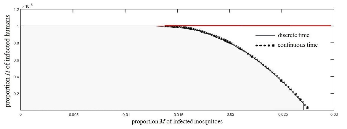
Figure 1: Viability kernels for the deterministic case: obtained by the dynamic programming Algorithm 1 in discrete time ($\mathring{\SS}=\{0.07660\}\times\{0.0722\}$, dotted line) and given by a mathematical formula in [10] in continuous time (broken starred line), for the infection cap $\overline{H}=0.00001=0.001\%$

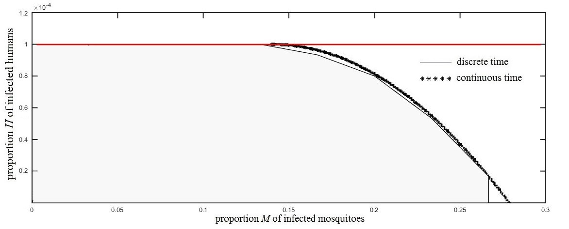
Figure 2: Viability kernels for the deterministic case: obtained by the dynamic programming Algorithm 1 in discrete time ($\mathring{\SS}=\{0.07660\}\times\{0.0722\}$, dotted line) and given by a mathematical formula in [10] in continuous time (broken starred line), for the infection cap $\overline{H}=0.0001=0.01\%$

We observe that the viability kernel for the deterministic case in discrete time is almost identical to the deterministic viability kernel in continuous time. Therefore, neither the sampling of controls and uncertainties — as described in §2.1 — nor the discretization process — described in §3.2 — lead to a degradation of the theoretical viability kernel.

Comparison between robust viability kernels as the set $\SS$ of uncertainties increases

In Figures 3 and 4, we display the three robust viability kernels corresponding to the three cases presented in §3.1: low case (deterministic) with $\SS=\mathring{\SS}$, middle case with $\SS=\overline{\SS}$ and high case with $\SS=\overline{\overline{\SS}}$.

For the middle case, we take

$$\overline{\SS}=[0,5]\times[0,25]~{}\text{day}^{-1}\times\text{day}^{-1}\;.$$ (31)

These numbers were obtained from the ranges for the parameters adjusted to the 2013 dengue outbreak in Cali, Colombia, as described in [10]. Details can be found in Appendix A.3.

For the high case, we doubled the right ends of each interval in (31), giving:

$$\overline{\overline{\SS}}=[0,10]\times[0,50]~{}\text{day}^{-1}\times\text{day}^{-1}\;.$$ (32)

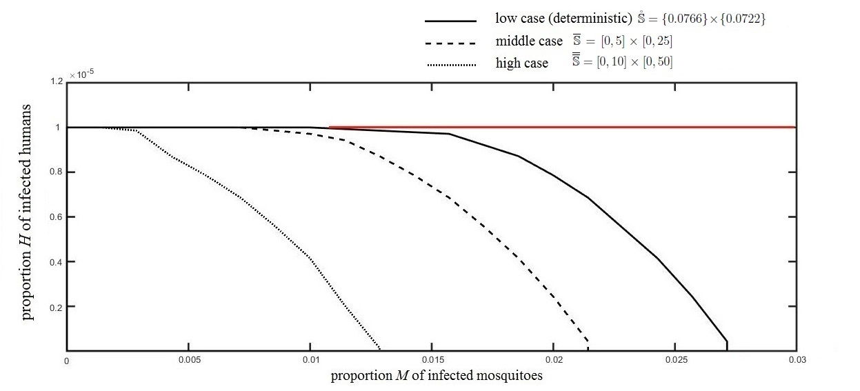
Figure 3: Deterministic viability kernel ($\mathring{\SS}=\{0.0766\}\times\{0.0722\}$, right hand side continuous line) and robust viability kernel for the middle case ($\overline{\SS}=[0,5]\times[0,25]$, middle broken line) and the high case ($\overline{\overline{\SS}}=[0,10]\times[0,50]$, left hand side dotted line), for the infection cap $\overline{H}=0.00001=0.001\%$

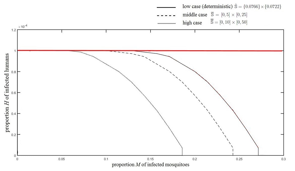
Figure 4: Deterministic viability kernel ($\mathring{\SS}=\{0.0766\}\times\{0.0722\}$, right hand side continuous line) and robust viability kernel for the middle case ($\overline{\SS}=[0,5]\times[0,25]$, middle broken line) and the high case ($\overline{\overline{\SS}}=[0,10]\times[0,50]$, left hand side dotted line), for the infection cap $\overline{H}=0.0001=0.01\%$

Discussion

In Figures 3 and 4 — both in the middle case (middle dashed line) and more markedly in the high case (left hand side dotted line) — we observe the following: a large part of the initial states $(M_{0},H_{0})$ that are identified as viable in the deterministic case (right hand side continuous line) are no longer viable when taking into account uncertainties.

In addition, as we expand the set $\SS$ where uncertainties take their values, the gap with the deterministic case is larger and larger. In the high case, when we double the extremites of $\overline{\SS}$, we observe in Figures 3 and 4 that all the initial states that are below the right hand side continuous line (boundary of the deterministic viability kernel) and above the lower left hand side dotted line no longer belong to the viability kernel. Thus, enlarging the set of uncertainties can have a strong impact on the viability kernel. When we have much variability in the values of the uncertain variables $(A_{m},A_{H})$, the robust viability kernel is greatly reduced.

Therefore, we cannot guarantee compliance with the constraint imposed on the proportion of infected humans for all uncertainties, if we take initial conditions belonging to the deterministic kernel. Picking initial conditions within the deterministic kernel would yield optimistic conclusions with respect to infection control, when uncertainties affect the epidemics dynamics.

These observations depend on the temporal horizon and on the structure of the set of scenarios. Recall that, in §2.3, we stressed the importance of having a rectangular set of scenarios to obtain a dynamic programming equation, making it possible to recursively compute robust viability kernels. This rectangularity property of the set of scenarios corresponds to stagewise independence of uncertainties: whatever the value of the uncertainty at time $t$, the next uncertainties can take any values (within the rectangle). This rectangularity property contributes to having small robust viability kernels. Indeed, scenarios can display arbitrary evolutions, switching from one extreme to another between time periods (days). High and low values for the uncertainties alternate, submitting the epidemics dynamics to a strong stress, and thus narrowing the possibility of satisfying the state constraints for all times. Such contrasted scenarios deserve the label of worst-case scenarios (they represent a small fraction of the extreme points of the rectangular set of scenarios). This is why amplifying the distance between extreme uncertainties shrinks the robust viability kernel.

4 Conclusion

In [10], the two authors obtained a neat expression of the deterministic viability kernel for a controlled Ross-Macdonald model. However, uncertainties abound and we wanted to assess their importance regarding epidemics control. The numerical results show that the viability kernel without uncertainties is highly sensitive to the variability of parameters — here the biting rate, the probability of infection to mosquitoes and humans, and the proportion of female mosquitoes per person. So, a robust viability analysis can be a tool to reveal the importance of uncertainties regarding epidemics control.

Appendix A Appendix. Fitting an epidemiological model for dengue

Here, we present how we identify parameters for the Ross-Macdonald model (1), and then obtain ranges for the uncertain aggregate parameters.

A.1 Parameters and daily data deduced from health reports

We introduce the vector of parameters

$$\theta=\big{(}\alpha,p_{h},p_{m},\xi,\delta\big{)}\in\Theta\subset\mathbb{R}^{5}_{+}\;,$$ (33)

consisting of the five parameters previously defined in Table 1. The parameter set $\Theta\subset\mathbb{R}^{5}_{+}$ is given by the Cartesian product of the five intervals in the third column of Table 2.

With these notations, the Ross-Macdonald model (1) now writes

$$\begin{array}[]{rl}\displaystyle\frac{dm(s;\theta)}{ds}&=\alpha p_{m}h(s;\theta)\big{(}1-m(s;\theta)\big{)}-\delta m\;,\\[14.22636pt] \displaystyle\frac{dh(s;\theta)}{ds}&=\alpha p_{h}\xi m(s;\theta)\big{(}1-h(s;\theta)\big{)}-\gamma h\;,\\[14.22636pt] \big{(}m(s_{0};\theta),h(s_{0};\theta)\big{)}&=(m_{0},h_{0})\;.\end{array}$$ (34)

Notice that the rate $\gamma$ of human recovery does not appear in the parameter vector $\theta$ in (33). Indeed, in the data provided by the Municipal Secretariat of Public Health (Cali, Colombia), we only have new cases of dengue registered per day; there is no information regarding how many inviduals recover daily. We choose an infectiousness period of 10 days, that is, a rate of human recovery fixed at

$$\gamma=0.1~{}\text{day}^{-1}\;.$$ (35)

Under this assumption, the daily incidence data (i.e., numbers of newly registered cases reported on daily basis) provided by the Municipal Secretariat of Public Health can be converted into the daily prevalence data (i.e., numbers of infected inviduals on a given day, be they new or not). With this, we deduce values of daily proportion of infected inviduals in the form of the set

$$\mathbb{O}=\Big{\{}\big{(}r,\hat{h}_{r}\big{)}\;,\enspace r=r_{0},r_{0}+1,\ldots,R\Big{\}}\;,$$ (36)

where $r$ refers to day $r$ within the observation period of $R+1-r_{0}$ days, and where $\hat{h}_{r}$ stands for the fraction of infected inviduals at day $r$. Naturally, the first couple in the set $\mathbb{O}$ in (36) defines the initial condition $h(r_{0};\theta)=\hat{h}_{0}$. Unfortunately, there is no available data for the fraction of infected mosquitoes. As mosquito abundance is strongly correlated with dengue outbreaks [13], we have chosen a relation $m(r_{0};\theta)=3\hat{h}_{0}$ at the beginning of an epidemic outburst (other choices gave similar numerical results).

A.2 Parameter estimation

To estimate a parameter vector $\theta\in\Theta$ in (33) that fits with the data provided by the Municipal Secretariat of Public Health we apply the curve-fitting approach based on least-square method. More precisely, we look for an optimal solution to the problem

$$\min\limits_{\theta\in\Theta}\sum_{r=r_{0}}^{R}\big{(}h(r;\theta)-\hat{h}_{r}\big{)}^{2}\;,\enspace R=60~{}\mbox{days}\;,$$ (37)

subject to the differential constraint (34). Regarding numerics, we have solved this optimization problem with the lsqcurvefit routine (MATLAB Optimization Toolbox), starting with an admissible $\theta^{(0)}\in\Theta$ (the exact value stands in the second column of Table 2). The routine generates a sequence $\theta^{(1)},\theta^{(2)}\ldots$ that we stop once it is stationary, up to numerical precision. For a better result, we have combined two particular methods (Trust-Region-Reflective Least Squares Algorithm [20] and Levenberg-Marquardt Algorithm [15]) in the implementation of the lsqcurvefit MATLAB routine.

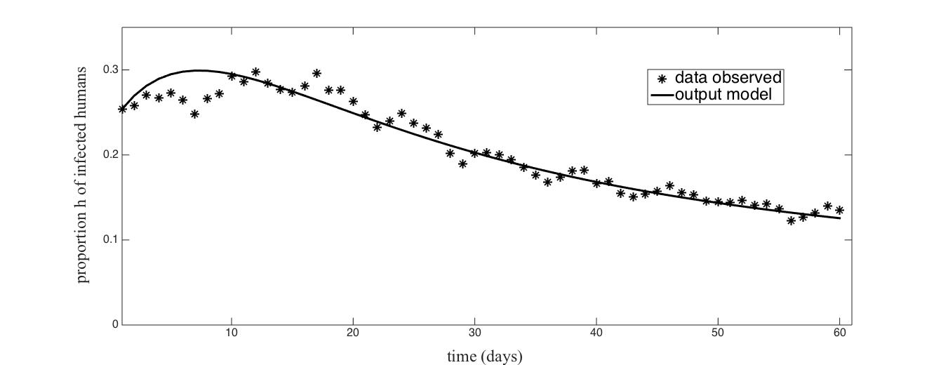
Figure 5: Fraction of inviduals infected with dengue, obtained by adjustment of the Ross-Macdonald model (1) (smooth solid curve) versus registered daily prevalence cases (star isolated points) during the 2013 dengue outbreak in Cali, Colombia

The last column of Table 2 provides estimated values for the parameters $\theta=\big{(}\alpha,p_{h},p_{m},\xi,\delta\big{)}$, and Figure 5 displays the curve-fitting results.

Parameter	Initial	Range	Reference	Estimated	Unit
	value			value
$\alpha$	1	$[0,5]$	[8], [17]	0.3600	$\text{day}^{-1}$
$p_{m}$	0.5	$[0,1]$		0.2128	dimensionless
$p_{h}$	0.5	$[0,1]$		0.1990	dimensionless
$\xi$	1	$[1,5]$	[14], [18]	1.0087	dimensionless
$\delta$	0.035	$\left[0.033,0.066\right]$	[8], [18]	0.0333	$\text{day}^{-1}$

Table 2: Initial values, admissible ranges, respective source references, estimated values of parameters (numerical solution of the optimization problem (37)–(34)) and units

Therefore, the aggregate parameters (2) are estimated as

$$A_{m}=0.076608~{}\text{day}^{-1}\;,\enspace A_{h}=0.0722633~{}\text{day}^{-1}\;.$$ (38a)

For the natural mortality rate $$\delta=\underline{u}$$ of mosquitoes (see Table 1), we obtain

$$\delta=\underline{u}=0.0333~{}\text{day}^{-1}\;.$$ (38b)

For the mosquito mortality maximal rate $$\overline{u}$$, we take

$$\overline{u}=0.05~{}\text{day}^{-1}\;.$$ (38c)

A.3 Ranges for the uncertain aggregate parameters

From the ranges for the parameters $\big{(}\alpha,p_{h},p_{m},\xi,\delta\big{)}$ displayed in the third column of Table 2, we obtain ranges for the aggregate parameters (2):

$$A_{m}=\alpha p_{m}\in[0,5]~{}\text{day}^{-1}\;,\enspace A_{h}=\alpha p_{h}\xi\in[0,25]~{}\text{day}^{-1}\;.$$ (39)

Acknowledgments.

The authors thank the French program PEERS-AIRD (Modèles d’optimisation et de viabilité en écologie et en économie) and the Colombian Programa Nacional de Ciencias Básicas COLCIENCIAS (Modelos y métodos matemáticos para el control y vigilancia del dengue, código 125956933846) that offered financial support for missions, together with École des Ponts ParisTech (France), Université Paris-Est (France), Universidad Autónoma de Occidente (Cali, Colombia) and Universidad del Valle (Cali, Colombia). We thank the Municipal Secretariat of Public Health (Cali, Colombia) for technical support and discussions. We are indebted to the editor-in-chief and to a reviewer, whose comments contributed to improve the manuscript.

References

- [1] R. M. Anderson and R. M. May. Infectious Diseases of Humans: Dynamics and Control. Oxford Science Publications. OUP Oxford, 1992.
- [2] J. Aubin. Viability theory. Systems & Control: Foundations & Applications. Birkhäuser Boston Inc., Boston, MA, 1991.
- [3] C. Béné and L. Doyen. Contribution values of biodiversity to ecosystem performances: A viability perspective. Ecological Economics, 68(1-2):14 – 23, 2008.
- [4] C. Béné, L. Doyen, and D. Gabay. A viability analysis for a bio-economic model. Ecological Economics, 36:385–396, 2001.
- [5] N. Bonneuil and K. Müllers. Viable populations in a prey-predator system. Journal of Mathematical Biology, 35(3):261–293, February 1997.
- [6] N. Bonneuil and P. Saint-Pierre. Population viability in three trophic-level food chains. Applied Mathematics and Computation, 169(2):1086 – 1105, 2005.
- [7] F. Brauer and C. Castillo-Chávez. Mathematical models in population biology and epidemiology, volume 40 of Texts in Applied Mathematics. Springer-Verlag, New York, 2001.
- [8] A. Costero, J. D. Edman, G. G. Clark, and T. W. Scott. Life table study of Aedes aegypti (diptera: Culicidae) in Puerto Rico fed only human blood plus sugar. Journal of Medical Entomology, 35(5), 1998.
- [9] M. De Lara and L. Doyen. Sustainable Management of Natural Resources. Mathematical Models and Methods. Springer-Verlag, Berlin, 2008.
- [10] M. De Lara and L. Sepulveda. Viable control of an epidemiological model. Mathematical Biosciences, 280:24–37, 2016.
- [11] O. Diekmann and J. A. P. Heesterbeek. Mathematical Epidemiology of Infectious Diseases. Wiley, Utrecht, Netherland, 2000.
- [12] H. W. Hethcote. The mathematics of infectious diseases. SIAM Review, 42:599–653, 2000.
- [13] C. C. Jansen and N. W. Beebe. The dengue vector Aedes aegypti: what comes next. Microbes and infection, 12(4):272–279, 2010.
- [14] F. Méndez, M. Barreto, J. Arias, G. Rengifo, J. Muñoz, M. Burbano, and B. Parra. Human and mosquito infections by dengue viruses during and after epidemics in a dengue-endemic region of Colombia. Am J Trop Med Hyg., 74(4):678–683, 2006.
- [15] J. J. Moré. The Levenberg-Marquardt algorithm: Implementation and theory. In G. A. Watson, editor, Numerical Analysis: Proceedings of the Biennial Conference Held at Dundee, June 28–July 1, 1977, pages 105–116. Springer Berlin Heidelberg, Berlin, Heidelberg, 1978.
- [16] E. Regnier and M. De Lara. Robust viable analysis of a harvested ecosystem model. Environmental Modeling & Assessment, 20(6):687–698, 2015.
- [17] T. W. Scott, P. H. Amerasinghe, A. C. Morrison, L. H. Lorenz, G. G. Clark, D. Strickman, P. Kittayapong, and J. D. Edman. Longitudinal studies of Aedes aegypti (diptera: Culicidae) in Thailand and Puerto Rico: Blood feeding frequency. Journal of Medical Entomology, 37(1):89, 2000.
- [18] T. W. Scott, A. C. Morrison, L. H. Lorenz, G. G. Clark, D. Strickman, P. Kittayapong, H. Zhou, and J. D. Edman. Longitudinal studies of Aedes aegypti (diptera: Culicidae) in Thailand and Puerto Rico: Population dynamics. Journal of Medical Entomology, 37(1):77, 2000.
- [19] D. L. Smith, F. E. McKenzie, R. W. Snow, and S. I. Hay. Revisiting the basic reproductive number for malaria and its implications for malaria control. PLoS Biol, 5(3):e42, 02 2007.
- [20] D. C. Sorensen. Newton’s method with a model trust region modification. SIAM Journal on Numerical Analysis, 19(2):409–426, 1982.